a 2-approximation algorithm for stochastic inventory...

A 2-Approximation Algorithm for Stochastic Inventory ControlModels with Lost Sales

Retsef LeviSloan School of Management, MIT, Cambridge, MA, 02139, USA

email: [email protected]

Ganesh JanakiramanIOMS-OM Group, Stern School of Business, New York University, New York, NY 10012, USA


Mahesh NagarajanSauder School of Business,University of British Columbia, Vancouver, BC V6T 1Z2, Canada


In this paper, we describe the first computationally efficient policies for stochastic inventory models with lost salesand replenishment lead times that admit worst-case performance guarantees.

In particular, we introduce dual-balancing policies for lost-sales models that are conceptually similar to dual-balancing policies recently introduced for a broad class of inventory models in which demand is backlogged ratherthan lost. That is, in each period, we balance two opposing costs: the expected marginal holding costs against theexpected marginal lost-sales cost. Specifically, we show that the dual-balancing policies for the lost-sales modelsprovide a worst-case performance guarantee of 2 under relatively general demand structures. In particular, theguarantee holds for independent (not necessarily identically distributed) demands and for models with correlateddemands such as the AR(1) model and the multiplicative auto-regressive demand model. The policies and theworst-case guarantee extend to models with capacity constraints on the size of the order and stochastic lead times.Our analysis has several novel elements beyond the balancing ideas for backorder models.

Key words: Inventory, Approximation ; Dual-Balancing ; Algorithms; Lost Sales

MSC2000 Subject Classification: Primary: 90B05 , ; Secondary: 68W25 ,

OR/MS subject classification: Primary: inventory/production , approximation/heuristics ; Secondary: produc-tion/scheduling , approximation/heuristics

1. Introduction In this paper, we address one of the fundamental problems in stochastic inventorytheory, the single-item, single location, periodic-review, stochastic inventory control problem with lostsales, which we refer to as the lost-sales problem. This problem has challenged researchers and practi-tioners for over five decades as very little is known about the structure of the optimal policy, and thereare no known provably good heuristics even for the simplest settings. We build on ideas first proposed byLevi, Pal, Roundy and Shmoys [5]. They proposed what are called dual-balancing policies for a class ofinventory models where unsatisfied demand is backlogged rather than lost. These policies have worst-caseperformance guarantees, that is, for each instance of the problem, the expected cost of the policy is guar-anteed to be at most C times the optimal expected cost (for some constant C). In this paper, we discussthe implementation and the worst-case analysis of dual-balancing policies applied to inventory modelswith lost sales. These models have mathematical characteristics that are very different than the modelsin which excess demand is backlogged and thus require a fundamentally different and novel worst-caseanalysis. In particular, we shall describe the first computationally efficient policies for inventory modelswith lost sales that have a worst-case performance guarantee of 2. The analysis is based on several newideas that we believe will contribute to future research in this domain.

Stochastic inventory theory provides streamlined models with the following common setting. The goalis to coordinate a sequence of orders over a planning horizon of finitely many discrete periods, aimingto supply a sequence of random demands over the planning horizon with minimum expected cost. Thecost consists of a per-unit ordering cost for ordering supply units at the beginning of each period (withor without capacity constraints), a per-unit holding cost for carrying excess inventory from one period tothe next, and a per-unit penalty cost for not satisfying demand on time. The dynamics of these models isas follows. At the beginning of each period, before the demand in this period is observed, a non-negativeprocurement order is placed with an outside supplier incurring a cost proportional to the number of unitsordered. This order will arrive and become available after a lead time of several periods. The demand inthat period is then observed and is satisfied to the maximum extent possible from the current inventory

1

2 :Mathematics of Operations Research xx(x), pp. xxx–xxx, c©200x INFORMS

on-hand. At the end of the period, two possible costs are incurred: excess units of inventory incur aproportional holding cost and unsatisfied units of demand incur a proportional penalty cost. The goal isto find an ordering policy that minimizes the overall expected costs over the entire horizon.

There are two common assumptions regarding unsatisfied demand at the end of a period. Thesedifferent assumptions distinguish between two fundamentally different classes of models. In the first classof models, the assumption is that unsatisfied units of demand will stay in the system, each incurring aper-unit penalty cost for each period until it is satisfied. That is, unsatisfied demand is backlogged fromperiod to period in a manner symmetric to excess inventory that is carried from period to period. Theseare called inventory models with backlogged demands. In the second class of models, which is the focusof this paper, each unsatisfied unit of demand is lost, i.e., it incurs a one-period penalty cost and thenleaves the system. While these two classes of models are equivalent if the lead time is equal to zero, thatis when the orders arrive instantaneously, they are fundamentally different for any positive lead time. Inparticular, the state-of-the-art knowledge on lost-sales models with lead times is very limited comparedto the well understood models with backlogged demands.

Dynamic programming has been the most dominant paradigm in studying stochastic inventory modelswith lost sales and backlogged demand (see Zipkin [15] and Section 2.1 below for dynamic programmingformulations of the lost-sales model). The optimization problem is defined recursively over time, usingsubproblems for each possible state of the system. In particular, the ordering decision in each period ismade based on the available information at the beginning, which includes the joint conditional distributionof future demands, additional information that may be available by that period and the pipeline vector.The pipeline vector consists of the inventory on-hand at the beginning of the period and the quantitiesof the outstanding orders that were placed in past periods and have not yet arrived. Clearly, the pipelinevector has length equal to the lead time, which suggests that the state space of the corresponding dynamicprogram can grow exponentially fast with the length of the lead time.

However, it turns out that in models with backlogged demands, it is sufficient to consider only the sumof the inventory on-hand at the beginning of the period (or any backlogged demand) and the quantitiesof the outstanding orders. This sum is usually called the inventory position of the system. The intuitionis that since all unsatisfied demands are backlogged, the impact of the decision made in the currentperiod on the future costs depends only on the difference between the inventory position of the system(after ordering) and the cumulative demand over the lead time (to be realized). Moreover, the optimalpolicies in the models with backlogged demands have a simple form and are called state-dependent base-stock policies. In each period, there is a target inventory position level, referred to as the base-stocklevel, which is unaffected by the specific pipeline vector. If at the beginning of the period the inventoryposition is below the target base-stock level, we order up-to that target. If the inventory position at thebeginning of the period is above the target base-stock level, no order is placed. The optimal base-stocklevels can be computed by solving the corresponding dynamic program. Since the inventory position isa “sufficient statistic” for the pipeline vector, the computational complexity of dynamic programs forbackorder models is insensitive to the lead time and is almost solely dictated by the complexity of thedemand structure. We refer the reader to [15, 10, 5] for proofs of the optimality of base-stock policiesand a discussion of the relevant literature regarding inventory models with backlogged demands.

In contrast, in systems with lost-sales systems and a positive lead time, the impact of the decisionmade in each period on the future costs is captured through a complicated mathematical expression thatdepends on the specific sequence of both the outstanding orders as well as the demands over subsequentperiods. Specifically, the optimal decision in each period depends on the entire pipeline vector and notonly on the inventory position as is the case in models with backlogged demands. As a result, the optimalpolicy in lost-sales models is significantly more complex and does not take the simple form of a base-stockpolicy and the inventory position is not a sufficient statistic for the pipeline vector. Moreover, the statespace of the corresponding dynamic program grows exponentially fast with the lead time.

Due to the aforementioned difficulties, the literature on lost-sales models is limited. Karlin and Scarf[4] have been the first to study the optimal policies for models with lost sales and positive lead times.They have considered a lost-sales model with discrete finite and infinite horizon and with independent,identically distributed demands. They have shown that a base-stock policy cannot be optimal. Fur-thermore, for the case where the lead time is equal to one period, they have partially characterized thestructure of the optimal policy. Specifically, they have shown that the optimal ordering quantity is a

:Mathematics of Operations Research xx(x), pp. xxx–xxx, c©200x INFORMS 3

decreasing function of the inventory on-hand at the beginning of the period, and is equal to zero outsidea specified interval. Moreover, the rate of decrease (as a function of the inventory on-hand) is strictlysmaller than one. With the additional assumption that demands are exponentially distributed, they havealso presented a steady-state analysis of the dynamics of lost-sales systems that use base-stock policies.Morton [8] has extended the analysis of Karlin and Scarf to lost-sales models with deterministic leadtimes. He has shown that the optimal ordering policy is a function of the entire pipeline with the follow-ing characteristics: (a) there is a compact region around the origin (that is, all the components of thepipeline vector are zero) such that the order quantity is strictly positive if and only if the pipeline vectoris in this region, (b) the order quantity decreases at a rate strictly between zero and one with respect toeach component of the pipeline vector and (c) the rate of decrease in the order quantity per componentis higher for components in the pipeline that are scheduled to arrive later in time. He has also derivedupper and lower bounds on the probability that the optimal policy will have enough inventory to meetdemand in the period in which the current order will arrive (a lead time ahead). Furthermore, he hasused these bounds to derive upper and lower bounds on the optimal ordering policy as a function of thecurrent pipeline vector. In a subsequent paper, Zipkin [17] has used state transformation techniques toestablish simpler proofs for the structure of optimal policies in the lost-sales models discussed in thispaper. Moreover, he has extended the results of Karlin and Scarf and Morton to models with capac-ity constrains on the size of the order, Markov modulated demands and stochastic lead times (with noorder-crossing).

Morton [9] has considered myopic policies for lost-sales models, in which, in each period, an order isplaced that minimizes the expected cost in the period in which this order arrives. There are other paperson lost-sales models like the ones by Nahmias [12] and Johansen [2] that propose different heuristics andpresent computational results on the performance of these heuristics. The computational experiments inall of these papers are restricted to instances where the lead time is short, equal to one or two periods orto models with extremely low demands. In a recent subsequent paper, Zipkin [16] presents computationalexperiments in which he tests the performance of several heuristics, including the dual-balancing policydescribed in this paper. He has focused on scenarios where the demands are independent and identicallydistributed; more specifically, they follow Poisson and Geometric distributions. Using state-reductiontechniques, he is able to compute the optimal policy for instances with lead time equal to 4. Computingoptimal policies with respect to instances with longer lead times seems very challenging. Moreover, tothe best of our knowledge, there is no heuristic for lost-sales models that has been shown to perform wellover a large bed of test problems of realistic size. Equally importantly, none of these papers provides aworst-case analysis of the proposed heuristics. Moreover, Levi, Pal, Roundy and Shmoys [5] have shownthat the myopic policy for the lost-sales model even with lead time equal to zero does not have worst-caseperformance guarantees. Specifically, they have shown a class of examples for which the myopic policyis arbitrarily more expensive than the optimal policy. Reiman has considered a model with continuoustime and with demand following a Poisson process and compared base-stock policies and policies thatplace an order in a fixed frequency [13].

In this paper we build on the recent work of Levi, Pal, Roundy and Shmoys [5] who have developed whatare called dual-balancing policies for a class of uncapacitated stochastic inventory models with backloggeddemands. These ideas have been extended to capacitated models [7] and multi-echelon models [6], againwith backlogged demands. These dual-balancing policies are computationally efficient and have a worst-case performance guarantee of 2 for the respective models under general assumptions on the demandstructure and the cost parameters. The dual-balancing policies are based on two novel ideas: a marginalcost accounting approach and cost balancing techniques. We note that the marginal cost accounting schemeis very different than the standard dynamic programming based cost accounting approach traditionallyused to analyze these models. Using the marginal cost accounting approach, the dual-balancing policy isbased on the repeated use of cost balancing techniques. In each period, two opposing (i.e. the holding andbacklogging) costs are balanced. The worst-case analysis in the above three papers is heavily based on themathematical properties of models with backlogged demands and uses a period-by-period amortizationcost of the dual-balancing policy with the cost of the optimal policy. Crucial to the analysis is the factthat in backorder models, comparing the inventory positions of any two policies in a period providessufficient information to analyze their respective performance a lead time ahead.

In this paper, we describe a dual-balancing policy for models with lost sales, which is conceptuallysimilar to the dual-balancing policy for models with backlogged demands. However, the above-mentioned


analysis for models with backlogged demand is not applicable to models with lost sales. In particular,the inventory position does not provide sufficient information to compare the costs of different policies.In addition, a period-by-period amortization of the cost of the dual-balancing policy with the cost of theoptimal policy does not seem useful. To overcome these difficulties, we describe a fundamentally differentanalysis which is based on two novel ideas. Rather than a period-by-period comparison, we use a globalamortization of the lost-sales costs of the dual-balancing policy with the lost-sales costs of the optimalpolicy. In addition, we introduce a new concept called the truncated inventory position which generalizesthe aforementioned notion of inventory position. As we have already mentioned, the inventory position ina certain period is defined to be the sum of the on-hand inventory at the beginning of the period plus alloutstanding orders. The truncated inventory position is defined to be the sum of the on-hand inventoryplus all the outstanding orders that have been ordered by a certain period, possibly earlier than thecurrent period. In other words, the truncated inventory position accounts for the on-hand inventory andall the outstanding orders that will arrive by a certain period. The new concept of truncated inventoryposition is used to compare two policies in a lost-sales system. Our main result is that the dual-balancingpolicy for the lost-sales model has a worst-case performance guarantee of 2.

The worst-case analysis holds for models with relatively general demand structures. For example,it holds under the assumption that the demands in different periods are independent, not necessarilyidentically distributed (see Section 3 below for details). Moreover, the analysis also holds in many modelsin which the demands in different periods are correlated; specifically, it holds in the multiplicative auto-regressive demand model and the AR(1) model, which are commonly used in the literature. Finally, thepolicy and the worst-case analysis extends to models with stochastic lead times (under the assumption of“no-crossing of orders”) and to models with capacity constraints on the size of the order in each period.

We note that the dual-balancing policy can be computed efficiently in most if not all of the realisticscenarios. As an example, we focus attention on the case where the demands are independent integer-valued random variables with bounded support, and provide a detailed analysis of the running time of thedual-balancing policy. Dynamic programming approach seems to be computationally intractable, sincethe running time grows exponentially fast in the lead time. In contrast, we show that the dual-balancingpolicy can be computed in time polynomial in the number of periods and the length of the support ofthe demands.

The rest of the paper is organized as follows. In Section 2, we describe the lost-sales model and adynamic programming formulation of the model. In Section 3, we describe a dual-balancing policy forlost-sales models and the new worst-case analysis under the assumption that the demands in differentperiods are independent. In Section 4, we discuss related computational issues of the dual-balancingpolicy. Finally, in Section 5 we describe several important extensions of the dual-balancing policy andthe worst-case analysis to models with capacity constraints on the size of the order, models with stochasticlead times and to models with demand structures that allow correlation between demands in differentperiods.

2. The Lost-Sales Model In this section, we provide the mathematical formulation of the lost-salesmodel and introduce some of the notation used throughout the paper.

As a general convention, we distinguish between a random variable and its realization using capitalletters and lower case letters, respectively. Script font is used to denote sets.

We consider a finite planning horizon of T periods numbered t = 1, . . . , T (note that t and T are bothdeterministic). There is a sequence of stochastic demands that occur over the planning horizon, which aredenoted by D1, . . . , DT , all of which have finite mean. We first assume that demands in different periodsare independent of each other, though not necessarily identically distributed. In Section 5 we shall showthat this assumption can be relaxed to allow several important structures of correlation between demandsin different periods.

As part of the model, we assume that at the beginning of each period s, there is an observed informa-tion set that is denoted by fs. The information set fs contains all of the information that is available atthe beginning of time period s. More specifically, the information set fs consists of the realized demands(d1, . . . , ds−1) over the interval [1, s) (in general fs can contain additional information that became avail-able by time period s). The information set fs in period s is one specific realization in the set of all


possible realizations of the random vector Fs = (D1, . . . , Ds−1). This set is denoted by Fs. We consideronly non-anticipatory policies, that is, in making a decision in period s, a feasible policy can use only theobserved information set fs.

In each period s = 1, . . . , T , a non-negative procurement order is placed from an outside supplier,incurring a per-unit ordering cost cs. The order placed in period s will arrive and become available onlyafter a positive lead time, denoted by L. We assume that L is a known positive integer, that is, an orderplaced in period s will arrive at the beginning of period s + L. (In Section 5, we will consider modelswhere the lead times are stochastic.)

We now describe the dynamics of the lost-sales model. At the beginning of each period s, as a functionof the observed information set fs, we observe the joint (conditional) distribution of future demands (ifdemands in different periods are independent of each other, then the joint distribution is fixed regardlessof the observed information set). At the beginning of period s, the system is characterized through thepipeline vector. The pipeline vector is denoted by Ps and consists of L components. The Lth componentis the inventory on hand (or on-hand inventory) available at the beginning of period s after the orderplaced L periods ago in period s−L has arrived and before the demand in period s is realized. We denotethe inventory on-hand at the beginning of period s by Is. The other L − 1 components of the pipelinevector are the outstanding orders that have been placed in previous periods and have not yet arrived.Specifically, the jth component of Ps is equal to Qs−j , the size of the order placed j periods ago, i.e., inperiod s− j (for j = 1, . . . , L− 1). That is,

Ps = (Qs−1, . . . , Qs+1−L, Is).

Observe that at the beginning of period s all the components of the pipeline vector are known determin-istically.

We next specify the sequence of events in each period s:

(i) The order of qs−L units placed in period s − L arrives and the on-hand inventory is thus is =(is−1 − ds−1)

+ +qs−L. Observe that (is−1−ds−1)+ is the inventory on-hand at the end of periods− 1.

(ii) Following a given policy, qs units are ordered (qs ≥ 0), and this incurs a cost of csqs. Next thedemand in period s is realized and is satisfied to the maximum extent possible from the inventoryon-hand. Since unsatisfied demand is lost and leaves the system, the on-hand inventory decreasesby min{ds, is}. In addition, we observe a new information set fs+1 ∈ Fs+1.

(iii) At the end of the period, costs are incurred. If (is − ds) > 0 then we incur a total holding costof hs(is − ds) (this means that there is excess inventory that needs to be carried to time periods + 1). On the other hand, if (is − ds) < 0 we incur a total lost-sales penalty cost of ps(ds − is)(this means that in period s there is unsatisfied demand that is lost).

For ease of exposition, we first assume that the cost parameters are stationary, that is, for eacht = 1, . . . , T , we have ht = h > 0, pt = p > 0 and ct = c ≥ 0. We further assume that c = 0. (Theworst-case analysis presented below holds for any c > 0.) We will show that in fact the analysis allowsus to have time-dependent holding costs parameters and non-increasing ordering and lost-sales penaltyparameters. In particular, the analysis holds for models with stationary cost parameters and discountfactor.

The goal is to find an ordering policy that minimizes the overall expected holding costs and lost-salespenalty costs over the entire horizon [1, T ]. We consider only policies that are non-anticipatory, i.e., attime s, the information that a feasible policy can use consists only of fs. Thus, for each feasible policy,given an information set fs, the pipeline vector at time period s and the order quantity in period s areknown deterministically.

2.1 Dynamic programming Formulation In this section, we discuss the dynamic programmingformulation of the lost sales model and discuss the associated difficulties in the analysis.

Observe that in a lost-sales model the cost in period s depends on the inventory on-hand at thebeginning of the period, that is, the expected cost in period s is equal to

E[h(Is −Ds)+ + p(Ds − Is)+].


Note that the decision made in period s of how many units to order affects only the costs over the interval[s+L, T ] (recall that the order placed in period s will arrive at the beginning of period s+L). Moreover,the impact of the decision in period s is captured through the effect it has on the inventory on-hand atthe beginning of period s + L. Unfortunately, in lost-sales models, there is no tractable way to capturethe impact of the decision in period s on the inventory on hand in period s+L. In particular, the impactof the decision made in period s on the inventory on-hand at the beginning of period s+L depends on thespecific sequence of both the outstanding orders at the beginning of period s and the realized demandsover the interval [s, s + L). Thus, the mathematical expressions of the dynamics of the lost-sales modelare quite involved. As we have already seen, for each t = 1, . . . , T ,

It+1 = (It −Dt)+ + Qt+1−L, (1)

which implies that the inventory on-hand in period s + L depends on the decision of how many unitsto order in period s through a complicated recursive expression. Thus, the resulting dynamic programformulation depends on the entire observed pipeline vector. Let Vs(ps, fs) = Vs((qs−1, . . . , qs+1−L, is), fs)be the optimal expected cost over the interval [s + L, T ] given an observed pipeline vector ps and anobserved information set fs. The recursion in the lost-sales model is

Vs((qs−1, . . . , qs+1−L, is), fs) = minqs≥0

{E[h(Is+L(qs)−Ds+L)+ + p(Ds+L − Is(qs))+|fs] + (2)

E[Vs+1((qs, qs−1, . . . , qs+2−L, (is −Ds)+ + qs+1−L), Fs+1)|fs]},

where Is+L(qs) is the inventory on-hand in period s + L assuming that in period s, we have ordered qs

units. It is readily verified that the state space of the above dynamic program grows exponentially fastin the length of the lead time L even in simple cases where the demands in different periods are assumedto be independent and identically distributed. This implies that solving the above dynamic program islikely to be intractable except for cases with very small lead times. Moreover, the dynamic program doesnot provide much insight on the structure of the optimal policies and this a main reason why theoreticalresearch on lost sales models is limited.

3. Dual-Balancing Policy for the Lost Sales Model In this section, we shall describe a dual-balancing policy for the lost-sales model, and then present a worst-case analysis that holds under relativelygeneral assumptions on the demand distributions D1, . . . , DT . We shall show that under these assump-tions, the dual-balancing policy has a worst-case performance guarantee of 2. That is, the expected costof the policy is guaranteed to be at most twice the expected cost of an optimal policy. In this section,we describe the dual-balancing policy and its worst-case analysis in the case where demands in differentperiods are assumed to be independent of each other, though not necessarily identically distributed. InSection 5 we discuss several important extensions of the dual-balancing policy and the worst-case analysisto more general models.

3.1 Dual-Balancing Policy The policy for the lost-sales model is conceptually similar to the oneproposed by Levi, Pal, Roundy and Shmoys for the model with backlogged demand [5]. That is, in eachperiod s, conditioned on the observed information set fs, we balance the (conditional) expected marginalholding cost incurred by the units ordered in that period over the entire horizon against the (conditional)expected lost-sales penalty cost incurred a lead time ahead in period s + L.

For a given policy P , let HPs be the marginal holding cost incurred by the units ordered in period s

over the entire horizon, and let ΠPs be the lost-sales penalty cost incurred in period s + L. The cost of

policy P can then be expressed as

C(P ) =T−L∑s=1

(HPs + ΠP

s ),

ignoring the marginal holding cost of units ordered before period 1 and the lost-sales penalty costs overthe interval [1, L] that are identical for every policy. However, the expressions of HP

s and ΠPs are different

in the lost-sales model, and are significantly more complex compared to the corresponding expressions inthe models with backlogged demands. Recall that IP

t is the on-hand inventory in period t after the orderplaced in period t−L has arrived and before the demand in period t has occurred. We have already seenthat, for each t = 1, . . . , T − 1,

IPt+1 = (IP

t −Dt)+ + QPt+1−L, (3)


(where QPj for j ≤ 0 are given as an input). Observe that (IP

t −Dt)+ is the inventory on-hand at theend of period t and QP

t+1−L is the order arriving at the beginning of period t + 1. Assuming without lossof generality that supply units are consumed on a first-ordered-first-consumed basis, we conclude thatthe QP

s units ordered in period s will be consumed only after all the (Is+L−1 − Ds+L−1)+ units thatwere on-hand at the beginning of period s + L (just before the order placed in period s has arrived) areconsumed. This leads to the following expression for the marginal holding cost incurred by the QP

s unitsordered in period s:

HPs =

T∑

t=s+L

h(QPs − (D[s+L,t] − (IP

s+L−1 −Ds+L−1)+)+)+. (4)

Similarly, we express

ΠPs = p(Ds+L − IP

s+L)+ = p(Ds+L − (QPs + (IP

s+L−1 −Ds+L−1)+))+, (5)

where the second equality follows from Equation (3) above. Equations (4) and (5) can be easily adaptedto capture time-dependent cost parameters. In addition, we can incorporate a linear ordering cost csQ

Ps

into Equation (4) above.

For each s = 1, . . . , T − L and an observed information set fs ∈ Fs, define the functions lBs (qBs ) =

E[HBs (qB

s )|fs] and πBs (qB

s ) = E[ΠBs (qB

s )|fs]. As in the dual-balancing policy for the model with back-logged demand [5], in each period s, conditioned on the observed information set fs, we order qB

s = q′sto balance lBs (q′s) = E[HB

s (q′s)|fs] = πBs (q′s) = E[ΠB

s (q′s)|fs]. It is readily verified that, conditioned onfs and the resulting pipeline vector pB

s , the functions lBs and πBs depend only on qB

s . Moreover, lBs isan increasing (convex) function of qB

s , which is equal to 0 if qBs = 0 and goes to infinity as qB

s goes toinfinity. In addition, πB

s is a (convex) decreasing function of qBs , which admits a non-negative value for

qBs = 0 and is going to 0 as qB

s goes to infinity. If fractional orders are allowed the function lBs and πBs

are continuous and thus q′s is well defined. (Later we shall discuss the case where orders are restricted tobe integral, and demands are integer-valued random variables.)

The intuition behind the idea of repeatedly balancing the functions πBs and lBs above is that in the

lost-sales model there are two underlying opposing risks, the risk of under ordering incurring lost-salespenalty cost and the risk of over ordering incurring holding costs. Balancing these two risks seems tobe very effective and computationally attractive. Surprisingly, this idea works significantly better thanminimizing the sum of the two functions. We also note that the dual-balancing policy can be implementedin an on-line manner. That is, the decision made in each period is not affected by any future decision ofthe policy, but only by the currently observed information set. This seems like an essential property ifone wishes to avoid the burden of solving huge dynamic programs. However, unlike myopic policy, whichin each period aims to minimize only the expected cost a lead time ahead, the dual-balancing policy doeslook ahead make use of available information about the future evolution of the system.

Integral orders and integer-valued demands. Next we discuss the case where the demands areinteger-valued random variables and the order quantity in each period is restricted to be an integer. Webriefly describe a randomized dual-balancing policy using ideas identical to ones used in [5, 7].

In this case, the functions lBs (qBs ) and πB

s (qBs ) are initially defined only for integer values. Their

piecewise linear interpolations preserve the monotonicity (and convexity) properties discussed in Section3. The problem is that the balancer q′s is likely to be fractional. Instead we consider the two consecutiveintegers q1

s ≤ q′s ≤ q2s . It is clear that q′s = λq1

s + (1 − λ)q2s for some 0 < λ < 1. We now order q1

s withprobability λ and q2

s with probability 1− λ.

3.2 Analysis - Independent Demands Given the dual-balancing policy for the lost-sales model,we define Zt to be the random balanced cost in period t, i.e., Zt = E[HB

t |Ft] = E[ΠBt |Ft] (for each

t = 1, . . . , T − L). Using an identical proof to the one in [5], we obtain the following lemma.

Lemma 3.1 The expected cost of the dual-balancing policy is equal to twice the sum of expectations of theZt variables, i.e., E[C(B)] = 2

∑T−Lt=1 E[Zt].

The worst-case analysis of the dual-balancing policy in models with backlogged demand [5] is basedon a period by period amortization of the cost of the dual-balancing policy against the optimal policy.


This is done by comparing the respective inventory positions of the the two policies, in each period [5].In contrast, it is well-known [15] that looking only on the inventory position is not sufficient to makeoptimal decisions in lost-sales models.

Similarly, unlike the analysis of the models with backlogged demands, comparing the inventory posi-tions of the dual-balancing policy and OPT in period s does not seem to provide ‘sufficient’ informationabout period s + L. For example, consider a lost-sales model with L = 1, where in period t the pipelinevector of policy 1 is p1

t = (3, 10) (i.e., on-hand inventory equal to 10 and an order of 3 units placed inperiod t) and the pipeline vector of policy 2 is p2

t = (4, 1) (i.e., on-hand inventory equal to 1 and an orderof 4 units placed in period t). In period t the inventory position of policy 1 is y1

t = 13, higher than theinventory position of policy 2, which is y2

t = 5. However, if the demand in period t is greater than 10,then policy 2 has greater on-hand inventory in period t+1 (4 units) than policy 1, which is left only with3 units on-hand. Conversely, if the demand in period t is no greater than 9, then policy 1 has on-handinventory in period t + 1 no smaller than that of policy 2.

The above example suggests that the period-by-period amortization scheme of the cost of the dual-balancing policy against the cost of OPT , based on the inventory position as used in the backlogginganalysis, does not seem to be useful when applied to the lost-sales model. (In models with backloggeddemand if one policy has a higher inventory position in period s, it will have higher on-hand inventory alead time ahead in period s + L.) To overcome this difficulty, the analysis presented below incorporatestwo novel ideas.

We use a global amortization of costs, that is, we compare the overall cost of the dual-balancing policyto that of OPT , where the comparison is not necessarily period-by-period. In addition, we introduce thenew concept of truncated inventory position, which is defined as follows. For each period s = 1, . . . , T ,the truncated inventory position with respect to period t (where t ∈ [s− L, s]), is defined to be the sumof the inventory on-hand in period s plus all outstanding orders placed by time period t. Let Yst denotethe truncated inventory position in period s with respect to period t, that is,

Yst = Is +t∑

j=s+1−L

Qj . (6)

Observe that the truncated inventory position Yst refers to the sum of the on-hand inventory in periods plus all outstanding orders that will arrive by time period t + L. Note that we consider a period tearlier than s which implies that all the orders that arrive by time period t + L are already known attime period s. Specifically, Yss = Ys is the traditional inventory position defined earlier in Section 2,and Ys,s−L = Is is the on-hand inventory at the beginning of period s. The truncated inventory positionis a generalization of the traditional inventory position concept commonly used in inventory theory (seeFigure 1). Due to the complex mathematical structure of lost-sales models, the effect of the decisionmade in the current period on future costs is very hard to quantify. The truncated inventory positionprovides a more tractable way to analyze this effect; specifically, the effect of the current ordering decisionon the on-hand inventory a lead time ahead. Moreover, it turns out that the concept of the truncatedinventory position provides the ‘right’ framework for comparing between the pipeline vectors of any twopolicies; specifically, OPT and the dual-balancing policy. Thus, a central part of the worst-case analysispresented below is based on this new concept. We believe that it will have more applications in othersettings.

The worst-case analysis in the model with backlogged demand is based on comparing the (traditional)inventory position of the dual-balancing policy and OPT in each period t, i.e., comparing Y B

tt and Y OPTtt .

Instead, in the lost-sales model, the analysis will be based on comparing the respective truncated inventorypositions Y B

st and Y OPTst in each period s ∈ [t, t+L]. That is, in each period s ∈ [t, t+L], we compare the

respective number of units already ordered by the dual-balancing policy and OPT that will be availableby time period t + L (see Figure.2).

Let TH be the set of all periods t ≤ T − L such that the truncated inventory of the dual-balancingpolicy with respect to period t is strictly smaller than the respective truncated inventory position of


Ps

P2s,s iy =−

P

1sq −

Psq

P

1s,sy −

Ps

Ps,s yy =

Figure 1: The truncated inventory position in period s (L=2).

OPT , for each period s ∈ [t, t + L]. That is,

TH = {t ≤ T − L : ∀ s ∈ [t, t + L], Y Bst < Y OPT

st }. (7)

Let TΠ be the complement of TH , i.e., the set of periods t ≤ T − L for which there exists somes ∈ [t, t + L] where the truncated inventory position of the dual-balancing policy with respect to periodt + L is no smaller than the respective truncated inventory position of OPT . That is,

TΠ = {t ≤ T − L : ∃ s ∈ [t, t + L] with Y Bst ≥ Y OPT

st }. (8)

Recall that in the lost-sales model, having a higher inventory position in period t does not guaranteehigher on-hand inventory in period t + L. Moreover, for certain realizations of the demands over theinterval [t, t + L), the truncated inventory position of the dual-balancing policy with respect to period tmight be higher than the respective truncated inventory position of OPT in some periods and lower inothers. In fact, it is possible to observe an alternating behavior, where the relation between the truncatedinventory position of the dual-balancing policy and that of OPT may change several times over theinterval. More precisely, for some period t and s ∈ [t, t + L), we will say that the respective truncatedinventory position of the dual-balancing policy with respect to period t and that of OPT alternate inperiod s if one of the following events occur

[Y Bst < Y OPT

st ] ∩ [Y Bs+1,t ≥ Y OPT

s+1,t ],

or[Y B

st ≥ Y OPTst ] ∩ [Y B

s+1,t < Y OPTs+1,t ].

That is, in the two consecutive periods s and s + 1, the inequalities relating the truncated inventorypositions of the dual-balancing policy and that of OPT alternate.

For each t ∈ TH , we know that in each period over the interval [t, t+L], OPT had (strictly) more unitsavailable by time period t+L. In particular, there is no alternation in the respective relation between thetruncated inventory position of the dual-balancing policy with respect to period t and that of OPT overthe interval [t, t+L). On the other hand, for each t ∈ TΠ, there was at least one period over that intervalwhen the dual-balancing policy had units available by time period t + L at least as many as OPT had.Note that this does not necessarily imply alternations (e.g., when the truncated inventory position of thedual-balancing policy with respect to period t is higher in period t and throughout (t, t + L]), nor doesit exclude more than one alternation (i.e., it is possible that the respective truncated inventory positionof OPT and that of the dual-balancing policy will alternate several times over [t, t + L)).

Next we state and prove two key lemmas that will show how to amortize the cost of the dual-balancingpolicy against the cost of OPT . The corresponding two lemmas hold with probability 1, i.e., for eachsample path of the demands D1, . . . , DT or equivalently, for each fT ∈ FT . (In the statements and proofs


Key

Order placed in this period Order placed 2 periods earlier

Order placed 1 period earlier Inventory on hand

t t+1 t+2 t+3

Pt,ty

Pt,1ty +

Pt,2ty +

Pt,3ty +

8d 1t =+ 0d 2t =+2d t =

Pti

P2tq −

P1tq −

Ptq

P1tq +

Ptq

P1tq −

P1ti +

P2ti +

Ptq

P1tq +

P2tq +

P3ti +

P1tq +

P2tq +

P3tq +

Figure 2: Evolution of the truncated inventory position with respect to period t over [t, t + L] (L = 3)


of these lemmas we shall omit the expression ‘with probability 1’.) In the first of these lemmas we willshow that the overall holding cost incurred by OPT , denoted by HOPT is greater than the holding costsincurred by units ordered by the dual-balancing policy in periods t ∈ TH .

Lemma 3.2 The holding cost incurred by OPT is greater than the holding cost incurred in the dual-balancing policy by units ordered in periods t ∈ TH , i.e., HOPT ≥ ∑

t∈THHB

t .

Proof. Recall that by definition Y Pt+L,t = IP

t+L. However, this implies that, for each t ∈ TH , we haveIBt+L < IOPT

t+L , i.e., the on-hand inventory of OPT in period t+L is higher than that of the dual-balancingpolicy. We have already seen that the on-hand inventory at the beginning of period t+L, just before theunits ordered in period t have arrived, is equal to (IP

t+L−1 −Dt+L−1)+. In particular,

IBt+L = QB

t + (IBt+L−1 −Dt+L−1)+ < IOPT

t+L .

Without loss of generality, we assume that supply units are consumed on a first-ordered-first-consumedbasis. We can then associate an index to each unit of supply currently on-hand according to the numberof units on-hand to be consumed prior to that unit (where units ordered in the same period are sortedarbitrarily). Note that since we allow fractional orders, the supply units are defined infinitesimally. Inparticular, the QB

t units ordered by the dual-balancing policy in period t are indexed in period t + L inthe range

((IBt+L−1 −Dt+L−1)+, (IB

t+L−1 −Dt+L−1)+ + QBs ]. (9)

Since t ∈ TH and the on-hand inventory of OPT in period t + L is higher, we conclude that in periodt + L there exist supply units on-hand in OPT with the same range of indices as in (9). We now matchpairs of units of supply with the same respective index (in period t + L) in the dual-balancing policy andOPT , respectively. In particular, in period t+L we match the supply units that are indexed in the aboverange in OPT to the QB

t units ordered by the dual-balancing policy in period t (see also Figure 3).

Observe that until the IBt+L units on-hand at the beginning of period t + L will be consumed, neither the

dual-balancing policy nor OPT incur lost-sales costs. Moreover, since the demands over [t + L, T ] arethe same for OPT and the dual-balancing policy, it is clear that each pair of respective matched supplyunits of OPT and the dual-balancing policy will incur the same holding cost over [t + L, T ], for eachsample path of demands Dt+L, . . . , DT . Since each pair of units are consumed at the same time period,it is readily verified that each supply unit of OPT can be matched to at most one supply unit of thedual-balancing policy. This concludes the proof. ¤

Note that the above proof still holds for time-dependent holding cost parameters and positive non-increasing per-unit ordering cost parameters, where the per-unit ordering cost is incorporated into themarginal expected holding cost and is balanced against the marginal expected lost-sales penalty cost.

In the second lemma, we amortize the lost-sales penalty costs of the dual-balancing policy which areassociated with periods t ∈ TΠ. In the proof of this lemma, we use a global amortization rather than aperiod-by-period one. For each t ∈ TΠ, we know that there exists some period s ∈ [t, t + L] such thatthe truncated inventory position of the dual-balancing policy with respect to period t is no smaller thanthe one of OPT , i.e., Y B

st ≥ Y OPTst . However, as we have already observed, this does not guarantee

that in period t + L the inventory on-hand of the dual-balancing policy is no smaller than the one ofOPT . That is, it is still possible to have IB

t+L < IOPTt+L , which implies that we can not amortize the

lost-sales penalty cost incurred by the dual-balancing policy in period t + L against the respective costof OPT in this period. The next lemma shows that in this case, period t + L belongs to an interval ofperiods over which the lost-sales penalty costs incurred by OPT are higher than the respective lost-salespenalty costs incurred by the dual-balancing policy. This leads to a global amortization of the cost ofthe dual-balancing policy with the cost of OPT .

Lemma 3.3 The lost-sales penalty incurred by OPT , denoted by ΠOPT , is greater than the lost-salespenalty costs of the dual-balancing policy which are associated with periods t ∈ TΠ, i.e.,ΠOPT ≥ ∑

t∈TΠΠB

t .


Mat

ched

Uni

ts

)( 11 DI LtOPT

Lt −+−+ − +

)( 11 DI LtB

Lt −+−+ − +

OPTt

Q

Bt

Q

BLt

I + OPTLt

I +

Figure 3: Matched supply units in period t + L where t ∈ TH .

Proof. Consider the following random partition of the periods L + 1, . . . , T . For each realizationof demands d1, . . . , dT , consider the resulting realization of the set TΠ, and partition the periods in thefollowing way. Start in period T and look for the latest period t ∈ TΠ with the property that period t+Lis not marked (initially all periods are unmarked) and iBt+L < iOPT

t+L (we abuse the notation and use TΠ todenote the deterministic set of periods resulting from the realized demands). If no such t exists then weterminate. If such a period exists, let t′ be that period and let wt′ be the earliest period in [t′, t′ + L] forwhich the truncated inventory position of the dual-balancing policy with respect to t′ is no smaller thanthe respective truncated inventory position of OPT . That is, wt′ = min{j ∈ [t′, t′ + L] : yB

jt′ ≥ yOPTjt′ }

(observe that wt′ is the realization of a random variable, denoted by Wt′ , which is defined for each periodt′ ∈ TΠ). By our assumption t′ does belong to TΠ, hence wt′ is indeed well-defined. We now mark all theperiods in [wt′ , t

′ + L]. Next we continue recursively over the periods 1, . . . , wt′ − 1. That is, we look forthe latest t ≤ wt′ − 1 such that t ∈ TΠ and with the property that t + L is unmarked and iBt+L < iOPT

t+L

and repeat the above.

The above procedure induces a random partition of the periods L+1, . . . , T into marked and unmarkedperiods, respectively. Let M be the (random) set of all marked periods. In particular, this randompartition induces a partition of the set TΠ into periods s ∈ TΠ such that s + L ∈M, i.e., s + L is markedand periods s ∈ TΠ such that s + L is not marked. First consider the latter set. For each period s ∈ TΠ

such that s+L /∈M, we know that IBs+L ≥ IOPT

s+L , for if not s+L would have been marked. This impliesthat for all periods {s ∈ TΠ : s + L /∈M}, we have ΠB

s ≤ ΠOPTs .

Now consider all the periods {s ∈ TΠ : s + L ∈ M}. Since all marked intervals are disjoint, it issufficient to show that, for each marked interval of the type [Wt′ , t

′ + L], the overall lost-sales penaltycosts incurred by OPT over that interval are higher than the respective lost-sales penalty costs incurredby the dual-balancing policy over that interval. In particular, this will imply that the lost-sales costs ofthe dual-balancing policy associated with periods in the set {s ∈ TΠ : s + L /∈ M} are lower than the


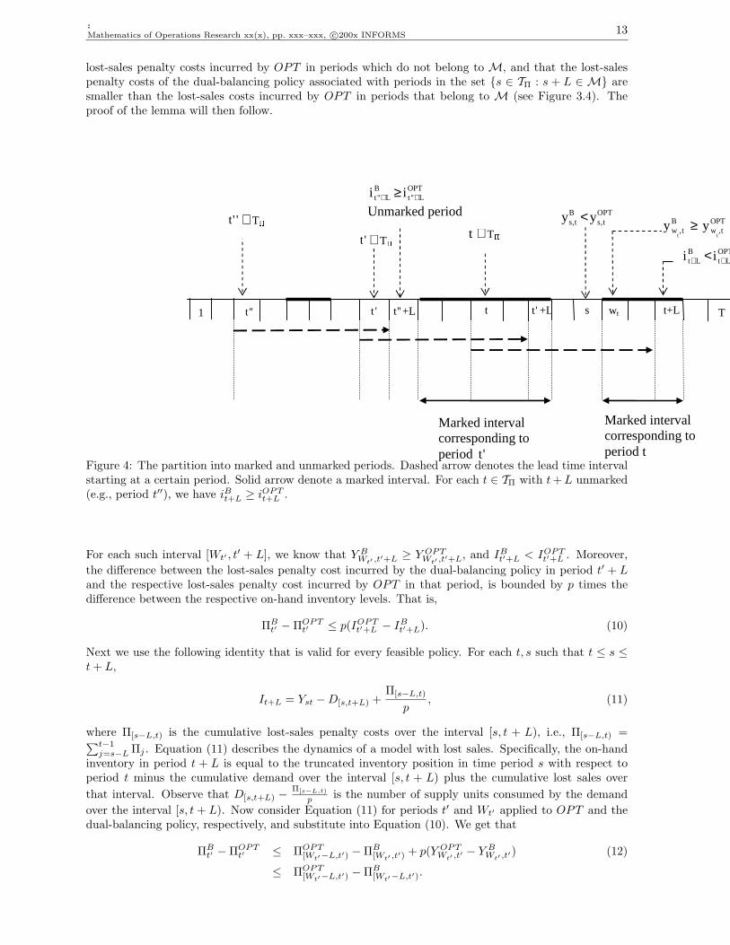
lost-sales penalty costs incurred by OPT in periods which do not belong to M, and that the lost-salespenalty costs of the dual-balancing policy associated with periods in the set {s ∈ TΠ : s + L ∈ M} aresmaller than the lost-sales costs incurred by OPT in periods that belong to M (see Figure 3.4). Theproof of the lemma will then follow.

T t+L wt

Marked interval corresponding to period t

't

Marked interval corresponding to period 't

t 1

t ∈T�

s ''t ''t +L

''t ∈T�

OPTL''t

BL''t ii ++ ≥

Unmarked period

OPTt,w

Bt,w

ttyy ≥

OPTLt

BLt ii ++ <

't +L

't ∈T�

OPTt,s

Bt,s yy <

Figure 4: The partition into marked and unmarked periods. Dashed arrow denotes the lead time intervalstarting at a certain period. Solid arrow denote a marked interval. For each t ∈ TΠ with t + L unmarked(e.g., period t′′), we have iBt+L ≥ iOPT

t+L .

For each such interval [Wt′ , t′ + L], we know that Y B

Wt′ ,t′+L ≥ Y OPTWt′ ,t′+L, and IB

t′+L < IOPTt′+L . Moreover,

the difference between the lost-sales penalty cost incurred by the dual-balancing policy in period t′ + Land the respective lost-sales penalty cost incurred by OPT in that period, is bounded by p times thedifference between the respective on-hand inventory levels. That is,

ΠBt′ −ΠOPT

t′ ≤ p(IOPTt′+L − IB

t′+L). (10)

Next we use the following identity that is valid for every feasible policy. For each t, s such that t ≤ s ≤t + L,

It+L = Yst −D[s,t+L) +Π[s−L,t)

p, (11)

where Π[s−L,t) is the cumulative lost-sales penalty costs over the interval [s, t + L), i.e., Π[s−L,t) =∑t−1j=s−L Πj . Equation (11) describes the dynamics of a model with lost sales. Specifically, the on-hand

inventory in period t + L is equal to the truncated inventory position in time period s with respect toperiod t minus the cumulative demand over the interval [s, t + L) plus the cumulative lost sales overthat interval. Observe that D[s,t+L) − Π[s−L,t)

p is the number of supply units consumed by the demandover the interval [s, t + L). Now consider Equation (11) for periods t′ and Wt′ applied to OPT and thedual-balancing policy, respectively, and substitute into Equation (10). We get that

ΠBt′ −ΠOPT

t′ ≤ ΠOPT[Wt′−L,t′) −ΠB

[Wt′ ,t′)+ p(Y OPT

Wt′ ,t′− Y B

Wt′ ,t′) (12)

≤ ΠOPT[Wt′−L,t′) −ΠB

[Wt′−L,t′).


The last inequality follows from the fact that Y BWt′ ,t′

≥ Y OPTWt′ ,t′

. We now get that∑

t∈TΠ

ΠBt =

∑

t:t∈TΠ, t+L∈MΠB

t +∑

t:t∈TΠ, t+L/∈MΠB

t (13)

≤∑

t:t∈TΠ, t+L∈MΠOPT

t +∑

t:t∈TΠ, t+L/∈MΠOPT

t ≤ ΠOPT .

This concludes the proof of the lemma. ¤We note that Lemma 3.3 holds also in the case where there are time-dependent lost-sales penalty

parameters p1, . . . , pT , as long as they are non-increasing. The proof is almost identical, but now wt′ isdefined to be the latest period j ∈ [t′, t′ + L], such that the cumulative lost sales of the dual-balancingover [j, t′ + L] is no higher than the corresponding lost sales of OPT over that interval. (The proof ofLemma 3.3 implies that the newly defined wt′ does exist.) This enables us to amortize the lost salesincurred by the dual-balancing policy, in each period t such that t− L ∈ TΠ, with lost sales incurred byOPT in periods earlier than t. (Specifically, for each period s ∈ [wt′ , t

′ + L], we amortize the lost salesof the dual-balancing in period s with lost sales of OPT incurred in periods [wt′ , s].) In particular, thelemma is valid in models with discounted costs.

Lemmas 3.2 and 3.3 imply that

HOPT + ΠOPT ≥∑

t∈TH

HBt +

∑

t∈TΠ

ΠBt .

Taking expectation we get that

E[C(OPT )] ≥ E[∑

t

(11(t ∈ TH) ·HBt + 11(t ∈ TΠ) ·ΠB

t )]. (14)

However, as we have already seen, in the lost-sales model the truncated inventory positions of the dual-balancing policy and OPT with respect to period t can alternate over the interval [t, t + L) from higherto lower. Thus, unlike the analysis of model with backlogged demand [5], conditioning on some ft ∈ Ft

does not necessarily realize the indicators 11(t ∈ TH) and 11(t ∈ TΠ) above. That is, it is possible that inperiod t we still do not know whether t ∈ TH or t ∈ TΠ.

Instead, we will condition on the events [t ∈ TH ] and [t ∈ TΠ], respectively, and get that

E[C(OPT )] ≥∑

t

E[E[11(t ∈ TH) ·HBt |Ft] + E[11(t ∈ TΠ) ·ΠB

t |Ft]] (15)

=∑

t

E[Pr(t ∈ TH |Ft) · E[HBt |(Ft, t ∈ TH)] + Pr(t ∈ TΠ|Ft) · E[ΠB

t |(Ft, t ∈ TΠ)]].

However, by conditioning on [t ∈ TH ] and [t ∈ TΠ], respectively, we consider information that super-sedes the original information set ft ∈ Ft based on which the dual-balancing policy has made the orderingdecision at the beginning of period t. That is, E[HB

t |(Ft, t ∈ TH)] and E[ΠBt |(Ft, t ∈ TΠ)] might not be

equal to E[HBt |Ft] = E[ΠB

t |Ft] = Zt. In particular, the problem arises for information sets ft ∈ Ft forwhich yB

tt < yOPTtt and the conditional probabilities (conditioning on ft) that [t ∈ TH ] and [t ∈ TΠ] are

both positive (If this is not the case, then we know whether t ∈ TH or t ∈ TΠ already at the beginning ofperiod t while observing ft.)

Next we will show that if the demands in different periods are independent of each other, then the twoinequalities

Pr(t ∈ TH |Ft) · E[HBt |(Ft, t ∈ TH)] ≥ Pr(t ∈ TH |Ft) · E[HB

t |Ft] (16)

and

Pr(t ∈ TΠ|Ft) · E[ΠBt |(Ft, t ∈ TΠ))] ≥ Pr(t ∈ TΠ|Ft) · E[ΠB

t |Ft] (17)

hold with probability 1, and this together with Equation (15) and the fact that Zt = E[HBt |Ft] =

E[ΠBt |Ft] imply that the dual-balancing has a worst-case performance guarantee of 2. Equations (16)

and (17) imply that conditioning also on the events [t ∈ TH ] and [t ∈ TΠ], respectively, implies that


the respective expected costs are even higher than what was expected at period t conditioning only onft. Note that this is the only part of the analysis that requires additional assumptions on the demanddistributions (beyond having finite mean). In Section 5, we shall generalize the analysis, and showthat Inequalities (16) and (17) hold under several other demand structures that incorporate correlationbetween demands in different periods. Intuitively, we require that the demands do not have a certain‘bad’ property. That is, we would like to exclude a situation where high demands over a certain intervalof periods, say (j′, j), imply low demands over the rest of the horizon [j, T ]. Indeed, if the demands areindependent, this ‘bad’ situation is excluded.

For each period t = 1, . . . , T − L and s ∈ [t, t + L), let Ast be the event that at the beginning ofperiod s the truncated inventory position of OPT with respect to period t is higher than the one ofthe dual-balancing policy, while at the beginning of period s + 1 the truncated inventory position of thedual-balancing policy with respect to period t is no smaller than the one of OPT . That is,

Ast = [Y Bst < Y OPT


s+1,t ].

Observe that conditioning on an information set ft such that yBtt < yOPT

tt , then t ∈ TΠ only if the eventAjt occurs for some j ∈ [t, t + L). In the next lemma we characterize some of the properties of the eventAst defined above.

Lemma 3.4 For each period t = 1, . . . , T −L and s ∈ [t, t + L), let Ast be as defined above. Suppose thatthe event Ast occurred. Then,

(i) The cumulative amount of orders placed by the dual-balancing policy over the interval [s +1 − L, t] is higher than the corresponding amount of orders of OPT over that interval, i.e.,∑t

j=s+1−L QBj ≥ ∑t

j=s+1−L QOPTj .

(ii) The inventory on-hand of OPT at the beginning of period s exceeds that of the dual-balancingpolicy by more than ∆Qs =

∑tj=s+1−L QB

j −∑t

j=s+1−L QOPTj , i.e., IOPT

s > IBs + ∆Qs .

(iii) The event Ast can be expressed as

[Y Bst < Y OPT

st ] ∩ [∆Qs ≥ 0] ∩ [Ds > IOPTs −∆Qs].

(iv) The dual-balancing policy has incurred positive lost sales in period s, and hence its on-handinventory at the beginning of period s+1 is equal to the size of the order placed in period s+1−L,denoted by QB

s+1−L. That is, Ast ⊆ [ΠBs−L > 0] ⊆ [IB

s+1 = QBs+1−L].

Proof. Recall Equation (6) that, for each policy P , we have Y Pst = IP

s +∑t

j=s+1−L QPj . Assume

that (i) does not hold, i.e., that Ast has occurred and that∑t

j=s+1−L QBj <

∑tj=s+1−L QOPT

j . SinceY B

st < Y OPTst , we conclude that IB

s − IOPTs <

∑tj=s+1−L QOPT

j −∑tj=s+1−L QB

j . However, it is readilyverified that this implies that the inventory on-hand of the dual-balancing policy at the end of period s,(IB

s − Ds)+, does not exceed the respective inventory on-hand of OPT , (IOPTs − Ds)+, by more than∑t

j=s+1−L QOPTj −∑t

j=s+1−L QBj . That is,

(IBs −Ds)+ − (IOPT

s −Ds)+ <

t∑

j=s+1−L

QOPTj −

t∑

j=s+1−L

QBj ,

which implies that Y Bs+1,t < Y OPT

s+1,t and leads to a contradiction. The proof of (i) then follows.

The proof of (ii) follows from (i) and the fact that Y Bst < Y OPT

st .

It is now clear that given (i) and (ii) above, the event Ast is equivalent to the event [Ds > IOPTs −∆Qs],

which implies (iii). Finally, (ii) and (iii) imply (iv). ¤In the next two lemmas we show that if the demands are independent of each other, then the Inequalities

(16) and (17) do hold. (We again omit the statement ‘with probability 1’ as long as the context is clear.)

Lemma 3.5 Assume that D1, . . . , DT are independent of each other. Then for each period t = 1, . . . , T −L, we have Pr(t ∈ TH |Ft) · E[HB

t |Ft] ≤ Pr(t ∈ TH |Ft) · E[HBt |(Ft, t ∈ TH)].


Proof. Consider some information set ft ∈ Ft. If Pr(t ∈ TH |ft) is equal either to 0 or to 1, thenthere is nothing to prove. Suppose now that 0 < Pr(t ∈ TH |ft) < 1. In particular, ft is such thatyB

tt < yOPTtt . It is now sufficient to show that E[HB

t |ft] ≤ E[HBt |(ft, t ∈ TH)].

Let Wt be the earliest period s ∈ [t, t + L] such that Y Bst ≥ Y OPT

st if such period exists and Wt = −1otherwise. It is readily verified that, conditioning on ft, the event [Wt = −1] is equivalent to the event[t ∈ TH ]. Note that the specific information set ft being considered implies that Pr(Wt = t|ft) = 0.Using conditional expectations, we now write

E[HBt |ft] = Pr(t ∈ TH |ft) · E[HB

t |(ft, t ∈ TH)] +t+L∑

j=t+1

Pr(Wt = j|ft) · E[HBt |(ft,Wt = j)]. (18)

It is now sufficient to show that, for each j = t + 1, . . . , t + L, E[HBt |ft] ≥ E[HB

t |(ft,Wt = j)]. Thistogether with Equation (18) imply that indeed E[HB

t |ft] ≤ E[HBt |(ft, t ∈ TH)] from which the proof

follows.

Recall, that conditioning on ft we know already the size of the order placed by the dual-balancing policyat the beginning of period t. Let φjt(ij) be the expected marginal holding cost of the qB

t = q′t units orderedby the dual-balancing policy in period t conditioning on ft and on the inventory on-hand at the beginningof period j equal to ij (for each j = t + 1, . . . , t + L). That is, φjt(ij) = E[HB

t |(ft, IBj = ij)]. Observe

that E[HBt |ft] = E[φjt(IB

j )|ft]. Since the demands in different periods are independent of each other, itis readily verified that Dj , . . . , DT are independent of IB

j and Ft. It follows from Equations (3) and (4)that φjt is increasing in ij . Moreover, IB

j |ft ≥ qBj−L (where qB

j−L is the size of the order arriving at thebeginning of period j, which conditioning of ft is known deterministically). Thus, φjt(IB

j )|ft ≥ φjt(qBj−L)

and E[φjt(IBj )|ft] ≥ φjt(qB

j−L). Finally, observe that the event ft ∩ [Wt = j] is also independent of thedemands Dj , . . . , DT . In addition, Lemma 3.4 above implies that the event ft∩[Wt = j] is contained in theevent Aj−1,t, i.e., contained in the event [IB

j = Qj−L]. We conclude that E[HBt |(ft,Wt = j)] = φjt(qB

j−L).This concludes the proof of the lemma. ¤

Lemma 3.6 Assume D1, . . . , DT are independent of each other. Then for each period t = 1, . . . , T − L,we have Pr(t ∈ TΠ|Ft) · E[ΠB

t |Ft] ≤ Pr(t ∈ TΠ|Ft) · E[ΠBt |(Ft, t ∈ TΠ)].

Proof. Consider an information set ft ∈ Ft. If Pr(t ∈ TΠ|ft) = 0 or Pr(t ∈ TΠ|ft) = 1, then thereis nothing to prove. Suppose that 0 < Pr(t ∈ TΠ|ft) < 1. In particular, ft is such that yB

tt < yOPTtt . Let

Wt be the same random variable as defined in Lemma 3.5 above. We express

E[ΠBt |(ft, t ∈ TΠ)] =

t+L∑

j=t

Pr(Wt = j|ft, t ∈ TΠ) · E[ΠBt |(ft,Wt = j, TΠ)]

=t+L∑

j=t

Pr(Wt = j|ft, t ∈ TΠ) · E[ΠBt |(ft,Wt = j)].

Since Pr(Wt = t|ft) = 0, it is sufficient to show, for each j = t + 1, . . . , t + L, that E[ΠBt |ft] ≤

E[ΠBt |(ft,Wt = j)].

For each j = t + 1, . . . , t + L, let ψjt(ij) be the expected lost-sales cost incurred by the dual-balancingpolicy in period t + L conditioning on ft and on the inventory on-hand at the beginning of period jequal to ij . That is, ψjt(ij) = E[ΠB

t |(ft, IBj = ij)]. Similar to Lemma 3.5 above, we conclude that ψjt is

decreasing in ij . This implies that

E[ΠBt |ft] = E[ψjt(IB

j )|ft] ≤ ψjt(qBj−L).

However, we have already observed that the event ft ∩ [Wt = j] is independent of the demandsDj , . . . , Dt+L, and is contained in the event Aj−1,t. From Lemma 3.4, we conclude that E[ΠB

t |(ft,Wt =j)] = ψjt(qB

j−L), from which the proof of the lemma follows. ¤Equation (15) and Lemmas 3.5 and 3.6 imply the following theorem.

Theorem 3.1 Consider the lost-sales model with independent demands, time-dependent holding cost pa-rameters and non-increasing ordering and lost-sales penalty parameters. Then the dual-balancing policyhas a worst-case performance guarantee of 2.


Randomized dual-balancing policy . Next we extend the worst-case analysis of the randomizeddual-balancing policy in the case where order quantities are restricted to be integers and the demandsare integer-valued random variables. Observe that now at the beginning of period s (conditioning on theobserved information set fs) we know q1

s and q2s above deterministically. However, the actual size of the

order is still random. Using the same definition of Zt above, it is readily verified that Lemma 3.1 is validand that E[C(B)] = 2

∑t E[Zt]. Next we modify the definition of the sets TH and TΠ and define them

with respect to the truncated inventory position of the dual-balancing policy assuming that it orders q2t

units (though it might end up ordering only q1t ). Denote this truncated inventory by Y B

st i.e., this is thetruncated inventory position of the dual-balancing policy in period s assuming that it has ordered q2

t

units in period t. In particular, 0 ≤ Y Bst − Y B

st ≤ 1. Specifically, we define

TH = {t ≤ T − L : ∀s ∈ [t, t + L] Y Bst ≤ Y OPT

st },and

TΠ = {t ≤ T − L : ∃s ∈ [t, t + L] Y Bst > Y OPT

st }.It is readily verified, that for each t ∈ TH , we have IB

t+L ≤ IOPTt+L , and that, for each t ∈ TΠ there exists

s ∈ [t, t + L] such that Y Bst ≥ Y OPT

st . Thus, all the arguments used in the proofs of Lemmas 3.2 and 3.3are still valid. The proofs of Lemmas 3.4, 3.5 and 3.6 directly apply.

4. Computational Issues Next we discuss several computational issues regarding the implemen-tation of the dual-balancing policy. The main goal of this discussion is to highlight the fundamentaldifference in the computational efforts required by the dual-balancing policy compared to the traditionaldynamic programming approach. The formal notion of computational efficiency in the context of stochas-tic optimization models is, by far, less clear than in deterministic optimization models. In particular, instochastic optimization models, one can make different assumptions regarding the way the probabilitydistributions are specified, and the oracles that are available, and each set of assumptions leads to adifferent analysis. Thus, a detailed analysis can be done only in the context of a concrete scenario. Inwhat follows, we shall restrict the discussion to two related issues:

(i) What oracles are needed in general for the implementation of the dual-balancing policy, and howthis is compared to the dynamic programming approach and the myopic policy.

(ii) A detailed analysis of the computational effort required to implement the dual-balancing policyin the important special case, where the demands D1, . . . , DT are independent (not necessarilyidentically distributed) integer-valued random variables with support within {0, . . . ,M}, whereM ∈ N. The goal is to highlight the fact that, in concrete and important scenarios, the dual-balancing policy can be implemented efficiently, whereas the dynamic programming approachdoes not seem to be tractable.

To implement the dual-balancing policy, we need to compute the balancer q′s in each period s =1, . . . , T − L. As a result, the running time of the dual-balancing policy is of the order T times thecomplexity of computing q′s in each period. The fact that q′s lies in the intersection of a decreasing(πB

s (qs)) and an increasing function (lBs (qs)) suggests that bisection search methods will be very efficientfor computing q′s as long as the functions lBs and πB

s above can be evaluated efficiently.

From Equations (4) and (5) above we can see that in order to evaluate the functions lBs and πBs it is

sufficient to be able to evaluate the distributions of D[s+L,t] (for each t = s + L, . . . , T ) and (IBs+L−1 −

Ds+L−1)+. The latter distribution is usually the most challenging one to evaluate. However, in periods conditioning on the observed information set fs, we already know deterministically the pipeline vectorpB

s including iBs , the on-hand inventory at the beginning of period s. Thus, we can use Equation (3) torecursively compute the distributions IB

s+1, IBs+2, . . . , I

Bs+L−1. Specifically, if there are efficient oracles to

evaluate the cumulative demand distributions D[s+L,t], for each s = 1, . . . , T − L and t ≥ s + L, and thedistributions (X −Ds)+, for each s = 1, . . . , T and a random variable X, then the functions πB

s and lBscan be evaluated efficiently.

This suggests that, in most if not all of the common scenarios, there exist efficient ways to evaluatethe functions lBs and πB

s . Note that the computational effort required grows moderately as the lead timeL grows. This is in contrast to the traditional dynamic programming approach that is very sensitive tothe lead time since the corresponding state space grows exponentially fast in the lead time L, even in


the simplest scenarios (see Section 2.1 above). In fact, the exponential growth of the state space makesit very hard to compute the optimal policies in models with lead times longer than 4 [16].

Moreover, the requirement to have an oracle that evaluates the distributions (X − Ds)+ above isessential even for computing a simple myopic policy. As we have already mentioned, this policy aims, ineach period s, to minimize the overall expected cost in period s+L [15, 16]. However, for computing themyopic policy one needs to evaluate the distribution (IB

s+L−1 −Ds+L−1)+.

Next we discuss the important special case in which the demands D1, . . . , DT are independent (notnecessarily identically distributed) integer-valued random variables with support over {0, . . . , M}, whereM ∈ N. We shall show how to compute the dual-balancing policy in time polynomial in T, L and M .

First, observe that like any reasonable policy the dual-balancing policy will never order more than Munits in a period. This implies that the inventory on-hand of the dual-balancing policy will never exceedM(L + 1). Moreover, the functions πB

s and lBs are piecewise linear with break points in the integers0, . . . , M . Thus, if there is an efficient way to evaluate the functions πB

s and lBs , one can compute thebalancer q′s using O(log M) calls for these functions. We simply apply a bisection search on {0, . . . ,M}to find the two consecutive integers q1

s and q2s = q1

s + 1 such that πBs (q1

s) ≥ lBs (q1s) and πB

s (q2s) ≤ lBs (q2

s).(Since the functions are piecewise linear, the balancer q′s can be expressed as a convex combination of q1

s

and q2s , and then the randomized dual-balancing can be applied.) It is now sufficient to show that one

can evaluate efficiently the functions πBs and lBs .

Focus on period s. Suppose that the cumulative distributions D[s+L,t] and the distribution of(IB

s+L−1 − Ds+L−1)+ are given explicitly, i.e., by specifying the values in the support and the corre-sponding probabilities. Since Ds+L, . . . , DT have support within {0, . . . , M} it follows that the supportof D[s+L,t] is within {0, . . . , TM}. Since all the orders and demands are integral, assuming that i0 is alsoan integer implies that (IB

s+L−1 −Ds+L−1)+ is an integer-valued random variables with support within{0, 1, . . . ,M(L+1)}. From Equations (4) and (5) it follows that, for a given order quantity qB

s , computingthe functions πB

s (qBs ) and lBs (qB

s ) can be done in O(T 2LM2) time. Specifically, lBs consists of a sum ofO(T ) elements, one for each period j = s + L, . . . , T . Each element j in the sum can be computed byenumerating over all the possible M(L+1) values of (IB

s+L−1 −Ds+L−1)+ and the possible TM values ofD[s+L,j]. For each j, this can be done in O(TLM2) time. Thus, the decision, in each period s, can becomputed in O(T 2LM2 log M) time.

Next we show how to construct the explicit distributions D[s+L,t] and (IBs+L−1−Ds+L−1)+. However,

if the distribution D[s+L,j] is given explicitly, we can construct the distribution D[s+L,j+1] in O(TM2)time. Thus, the cumulative demand distributions can be computed recursively in O(T 2M2) time. Recallthat conditioning on fs we know iBs . The recursive Equation (3) and the fact that D1, . . . , DT are integer-valued random variables with support within {0, . . . , M} imply that, for each j = 0, . . . , L−1, the randomvariable (IB

s+j −Ds+j)+ has at most (j + 1)M + 1 values in its support. Moreover, if (IBs+j −Ds+j)+ is

given explicitly, we can compute the explicit distribution of (IBs+j+1 − Ds+j+1)+ in O(jM2). Since we

use the recursion of Equation (3) L− 1 times, it follows that the distribution of (IBs+L−1−Ds+L−1)+ can

be expressed explicitly in O(M2L2). This implies the following theorem.

Theorem 4.1 Consider the lost-sales model with integer-valued independent demands D1, . . . , DT withsupport within {0, . . . , M}, for some M ∈ N. Then the dual-balancing policy can be computed inO(T 2LM2 log M) time.

We note that computing an optimal policy in the above scenarios seems extremely hard unless the leadtime is very short. There are many other scenarios in which the dual-balancing policy can be computedefficiently. The specific analysis requires detailed specifications of the underlying assumptions. We believethat in most of the common scenarios, the dual-balancing policy proposed above will be straightforwardto implement both computationally and conceptually.

5. Extensions

5.1 Infinite Horizon In this subsection, we briefly discuss the implementation of the dual-balancingpolicy in models with infinite horizon. Conceptually, the dual-balancing policy can still be implemented.However, the computational effort involved depends on the maximum number of periods that a unit


ordered in some period can stay in inventory before consumed. (This will affect the computation of themarginal holding costs.) Finally we note that the same worst-case analysis described in Section 3 abovestill holds in infinite horizon models with average or discounted cost.

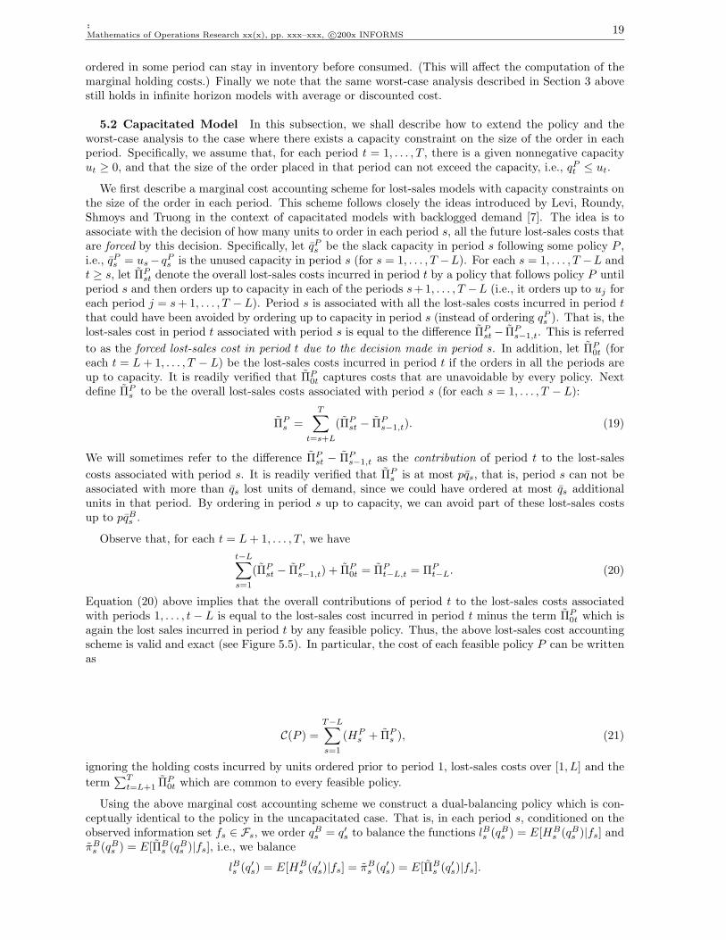
5.2 Capacitated Model In this subsection, we shall describe how to extend the policy and theworst-case analysis to the case where there exists a capacity constraint on the size of the order in eachperiod. Specifically, we assume that, for each period t = 1, . . . , T , there is a given nonnegative capacityut ≥ 0, and that the size of the order placed in that period can not exceed the capacity, i.e., qP

t ≤ ut.

We first describe a marginal cost accounting scheme for lost-sales models with capacity constraints onthe size of the order in each period. This scheme follows closely the ideas introduced by Levi, Roundy,Shmoys and Truong in the context of capacitated models with backlogged demand [7]. The idea is toassociate with the decision of how many units to order in each period s, all the future lost-sales costs thatare forced by this decision. Specifically, let qP

s be the slack capacity in period s following some policy P ,i.e., qP

s = us− qPs is the unused capacity in period s (for s = 1, . . . , T −L). For each s = 1, . . . , T −L and

t ≥ s, let ΠPst denote the overall lost-sales costs incurred in period t by a policy that follows policy P until

period s and then orders up to capacity in each of the periods s+1, . . . , T −L (i.e., it orders up to uj foreach period j = s + 1, . . . , T −L). Period s is associated with all the lost-sales costs incurred in period tthat could have been avoided by ordering up to capacity in period s (instead of ordering qP

s ). That is, thelost-sales cost in period t associated with period s is equal to the difference ΠP

st− ΠPs−1,t. This is referred

to as the forced lost-sales cost in period t due to the decision made in period s. In addition, let ΠP0t (for

each t = L + 1, . . . , T − L) be the lost-sales costs incurred in period t if the orders in all the periods areup to capacity. It is readily verified that ΠP

0t captures costs that are unavoidable by every policy. Nextdefine ΠP

s to be the overall lost-sales costs associated with period s (for each s = 1, . . . , T − L):

ΠPs =

T∑

t=s+L

(ΠPst − ΠP

s−1,t). (19)

We will sometimes refer to the difference ΠPst − ΠP

s−1,t as the contribution of period t to the lost-salescosts associated with period s. It is readily verified that ΠP

s is at most pqs, that is, period s can not beassociated with more than qs lost units of demand, since we could have ordered at most qs additionalunits in that period. By ordering in period s up to capacity, we can avoid part of these lost-sales costsup to pqB

s .

Observe that, for each t = L + 1, . . . , T , we havet−L∑s=1

(ΠPst − ΠP

s−1,t) + ΠP0t = ΠP

t−L,t = ΠPt−L. (20)

Equation (20) above implies that the overall contributions of period t to the lost-sales costs associatedwith periods 1, . . . , t− L is equal to the lost-sales cost incurred in period t minus the term ΠP

0t which isagain the lost sales incurred in period t by any feasible policy. Thus, the above lost-sales cost accountingscheme is valid and exact (see Figure 5.5). In particular, the cost of each feasible policy P can be writtenas

C(P ) =T−L∑s=1

(HPs + ΠP

s ), (21)

ignoring the holding costs incurred by units ordered prior to period 1, lost-sales costs over [1, L] and theterm

∑Tt=L+1 ΠP

0t which are common to every feasible policy.

Using the above marginal cost accounting scheme we construct a dual-balancing policy which is con-ceptually identical to the policy in the uncapacitated case. That is, in each period s, conditioned on theobserved information set fs ∈ Fs, we order qB

s = q′s to balance the functions lBs (qBs ) = E[HB

s (qBs )|fs] and

πBs (qB

s ) = E[ΠBs (qB

s )|fs], i.e., we balance

lBs (q′s) = E[HBs (q′s)|fs] = πB

s (q′s) = E[ΠBs (q′s)|fs].


t td tq tq− 1 1 1( )t t t ti i d q+− − −= − + Lost sales in

period t ~

tΠ tΠ

1 2 3 5 5 0 4 2 2 8 5 3 6 2 2�1 3 0 3 3 4 2 5 0 2 4

2�1 3�2

4 13 - - 6 7

2�3

0 0

Figure 5: A specific sample-path of demands and orders (L = 1, p = 1). An arrow indicates an allocationof units of shortage to a period. For example, in period 4 there are 7 units of lost sales, out of which 2units of shortage are associated with period 3 (i.e., Π34 − Π24 = 2), 3 units are associated with period 2(i.e.,Π24 − Π14 = 3) and 2 units are associated with period 1 (i.e., Π14 − Π04 = 2). The last two columnscompare the lost-sales costs associated with each period according to the traditional and marginal costaccounting, respectively.In particular, we again balance the expected marginal holding costs incurred by the units ordered inperiod s against the expected marginal future lost-sales costs forced by the decision in period s. Notethat the function πB

s is nonnegative at qBs = 0 and is equal to 0 at qB

s = us. Thus, the balancer q′sabove is again well-defined. Note that the function πB

s is more complicated to evaluate compared to πBs ,

the period expected lost-sales cost incurred in period s + L, defined above for the uncapacitated model.However, in most common scenarios it is still relatively straightforward to evaluate it accurately andefficiently. Observe that in the uncapacitated model, all the capacities are equal to ∞ and thus, qP

s = ∞.It is now readily verified that in this case ΠP

s = ΠPs . That is, the marginal lost-sales cost accounting

scheme for the capacitated model is in fact a generalization of the traditional lost-sales cost accountingscheme for uncapacitated models.

The worst-case analysis is very similar to the analysis presented in Section 3 above for the uncapacitatedmodel. In particular, defining Zt = E[HB

t |Ft] = E[ΠBt |Ft], it is readily verified that Lemma 3.1 is still

valid. That is, E[C(B)] = 2∑

t E[Zt]. We also keep the definitions of the sets TH and TΠ the same asbefore. It is easy to see that Lemma 3.2 above is still valid, that is, HOPT ≥ ∑

s∈THHB

s . Next we stateand prove a lemma analogous to Lemma 3.3.

Lemma 5.1 The lost-sales penalty incurred by OPT , denoted by ΠOPT , is greater than the lost-salespenalty costs of the dual-balancing policy which are associated with periods s ∈ TΠ, i.e.,ΠOPT ≥ ∑

s∈TΠΠB

s .

Proof. As in Lemma 3.3 we first describe a random partition of the periods L+1, . . . , T . Specifically,consider a realization of the demands d1, . . . , dT . Look for the latest period t with iBt < iOPT

t thatcontributes to the lost-sales costs associated with some period s ∈ TΠ. That is, ΠB

st− ΠBs−1,t > 0 for some

s ∈ TΠ. If no such t exists terminate. Otherwise, let t′ be that period and let s′ be the latest period inTΠ within the interval [1, t′ − L]. Note that since t′ contributes lost-sales costs only to periods within[1, t′ − L] including some period s ∈ TΠ within that interval, s′ above is well-defined. However, it is notnecessary that t′ contributes lost-sales costs to s′ itself. Let ws′ be the earliest period in [s′, s′ + L], suchthat Y B

ws′ ,s′≥ Y OPT

ws′ ,s′(since s′ is in TΠ, ws′ is well-defined). Next mark all the periods in [ws′ , t

′]. As inLemma 3.3 we repeat the above for the interval [1, ws′).

This induces a partition of the periods that contributes to the lost-sales costs associated with periodss ∈ TΠ into marked and unmarked periods. Consider first an unmarked period t that contributes to thelost-sales costs associated with periods s ∈ TΠ. By the definition of the partition described above, it isreadily verified that IB

t ≥ IOPTt , thus, ΠOPT

t−L ≥ ΠBt−L (i.e., the lost sales incurred by OPT in period t is

higher than the respective lost-sales costs of the dual-balancing policy). Moreover, Equation (20) impliesthat the lost-sales cost incurred by OPT in period t is higher than all the lost-sales costs incurred bythe dual-balancing policy in period t, which are associated with periods 1, . . . , t − L. In particular, thelost-sales cost OPT incurs in period t is higher than all of the contributions of period t to periods s ∈ TΠ.It is now sufficient to show that the lost-sales costs incurred by OPT over an interval [ws′ , t

′] are higherthan the lost-sales costs incurred by the dual-balancing policy over that interval, which are associated


with periods s ∈ TΠ. Observe that by the definition of the partition all of these periods are within theinterval [1, s′]. For each such interval, we have (we again abuse notation and use s′, t′ and ws′ thoughthey are random variables),

ΠOPTt′−L

p= (Dt′ − IOPT

t′ )+ ≥ Dt′ − IOPTt′

= Dt′ − (Y OPTws′ ,s′

+∑

j∈(s′,t′−L]

qOPTj −D[ws′ ,t′) +

ΠOPT[ws′−L,t′−L)

p),

where the equality follows again from the identity

IOPTt = Y P

ws,s +∑

j∈(s,t−L] qOPTj −D[ws,t) +

ΠOP T[ws−L,t−L)

p for each t, s ≤ t−L and ws ∈ [s, s + L]. TakingΠOP T

[ws−L,t−L)

p to the left-hand side, we get

ΠOPT[ws′−L,t′−L]

p≥ Dt′ − (Y B

ws′ ,s′+

∑

j∈(s′,t′−L]

uj −D[ws′ ,t′))

= Dt′ − (Y Bws′ ,s′

+∑

j∈(s′,t′−L]

uj −D[ws′ ,t′) +ΠB

[ws′−L,s′]

p+

∑

r∈(s′+L,t′)

ΠBs′r

p)

+ΠB

[ws′−L,s′]

p+

∑

r∈(s′+L,t′)

ΠBs′r

p=

ΠB[ws′−L,s′]

p+

∑

r∈(s′+L,t′]

ΠBs′r

p.

The first inequality follows from the fact that Y Bws′ ,s′

≥ Y OPTws′ ,s′

and uj ≥ QOPTj . In the first equality we

just add and subtractΠB

[ws′−L,s′]

p +∑

r∈(s′+L,t′)ΠB

s′rp . Here

ΠB[w

s′−L,s′]p is as before the lost sales incurred

by the dual-balancing policy over the interval [ws′ , s′ + L] and

∑r∈(s′+L,t′)

ΠBs′rp is the lost sales incurred

over (s′ + L, t′) by a policy that follows the dual-balancing policy until period s′ and then orders up tocapacity in periods s′ + 1, . . . , T − L. The last equality follows from the fact that

Dt′ − (Y Bws′ ,s′

+∑

j∈(s′,t′−L]

uj −D[ws′ ,t′) +ΠB

[ws′−L,s′]

p+

∑

r∈(s′+L,t′)

ΠBs′r

p)

is equal to the lost sales that the above policy incurs in period t′, i.e., equal to ΠBs′t′ . In particular, observe

that this policy has the same truncated inventory position in period ws′ with respect to period s′, and

over the time interval [ws′ , s′ + L) it incurs exactly

ΠB[w

s′−L,s′)p units of lost sales (this policy follows the

dual-balancing until period s′).

Finally, we have already seen that the part of the lost-sales costs incurred by the dual-balancing policyover the time interval [ws′ , s

′ + L] that is associated (by the marginal cost accounting scheme) withordering decisions in other periods can not exceed the actual lost-sales cost incurred over this interval,i.e., ΠB

[ws′−L,s′] (see also Equation (20) above). Moreover, from Equation (19) it follows that the part ofthe lost-sales costs incurred by the dual-balancing policy in some period t ∈ [s′ + L, t′] that is associated(by the marginal cost accounting scheme) with the an ordering decision in some period s ∈ [1, s′] can notexceed ΠB

st, which is the lost sales incurred in period t by a policy that follows the dual-balancing policyuntil period s and then orders up to capacity in each of the subsequent periods. However, by definitionthis is at most ΠB

s′t, which is similarly, the lost-sales cost incurred in period t by a policy that follows thedual-balancing policy until period s′, and only then starts to order up to capacity. The last step of theproof is identical to Equation (13) in the proof of Lemma 3.3 above (see Figure 5.6).

¤Similar to the uncapacitated model discussed in Section 3, the proof of the Lemma 5.1 can be extended

to models with non-increasing lost-sales penalty parameters. Observe that Lemmas 3.4 and 3.5 still hold.In addition, it can be verified that Lemma 3.6 still holds with respect to ΠB

t (instead of ΠBt ), i.e.,


j T t'-L

1

s 'sw t' s'

}Tj:L'tjmax{s' Π∈−≤=

OPT't

B't ii <

Marked interval Next marked interval

s'+L

OPT]L't,L'sw[]'t,L's(r

Br's

B]'s,L'sw[

~−−+∈−

Π≤∑Π+Π

OPTj

Bj ii ≥

k

0~~

0~~

0'~

'~

Ts

Bj,1s

Bj,s

Bk,1s

Bk,s

Bt,1s

Bt,s

>Π−Π

>Π−Π

>Π−Π

∈

−

−

−

Π

Figure 6: Period s is associated with lost-sales costs from periods j, k and t′. Period j is unmarked,thus, the lost sales costs of OPT can pay for all the contributions of period j to other periods. Periodsk and t′ are within a marked interval, thus, the lost-sales costs of OPT over the interval can pay for allthe contributions to periods in [1, s′].

E[ΠBt |ft] ≤ E[ΠB

t |(ft,Wt = j)] for each t = 1, . . . , T − L and j ∈ (t, t + L]. Thus, we get the followingtheorem.

Theorem 5.1 The dual-balancing policy for the capacitated lost-sales model with independent demands,time-dependent holding cost parameters and non-increasing ordering and lost-sales penalty parametershas a worst-case guarantee of 2.

Finally, we note that the above analysis still holds if the capacities, in each period are random, andfollow an exogenous stochastic process. (The only difference is that now the expectations are taken withrespect to the random future demands and capacities.)

5.3 Stochastic Non-crossing Lead Times In this subsection, we shall show how the dual-balancing policy and its worst-case analysis can be extended to the lost-sales model with stochasticlead times. Specifically, we assume that the stochastic lead times are such that orders do not cross orovertake each other; that is, for every realization of lead times, the order placed in a period arrives nolater than any subsequent order. Such lead time models have been first introduced by Kaplan [3] andsubsequently streamlined by Nahmias [12]. For ease of exposition we consider the uncapacitated model.

For each t = 1, . . . , T , let Lt be the stochastic lead time of the order placed in period t, which is realizedat time period t + Lt. The stochastic process {Lt}t has the property that {t + Lt} is a non-decreasingsequence for every sample path (i.e., with probability 1). We also assume that the processes {Lt}t and{Dt}t are independent of each other.

We will now explain how the definitions, results and proofs discussed in Section 3 above have to bemodified to extend the dual-balancing policy and the analysis to the more general model with stochasticlead time.

The dynamics of the inventory-on-hand process is now reflected by the following modified version of


equation (3).

IPt+1 = (IP

t −Dt)+ +∑

r:r+Lr=t+1

QPr . (22)

Next, the marginal holding cost incurred by the units ordered in period s, denoted again by HPs , is

still given by equation (4) after replacing L with Ls, the stochastic lead time of an order placed in s.

Note that, in the model with stochastic lead times, there are no orders delivered in the time interval(t + Lt, t + 1 + Lt+1) even if t + Lt < t + 1 + Lt+1. The lower and upper ends of this interval arethe periods in which the respective orders placed in periods t and t + 1 are delivered. In particular, ift+Lt < t+1+Lt+1, then once the decision of how many units to order in period t is made, the lost-salescosts over [t + Lt, t + 1 + Lt+1) are just a function of future demands and are not affected by any futuredecision. Thus, we define ΠP

s to be the marginal lost-sales costs associated with period t,

ΠPt = p

∑

r∈[t+Lt,t+1+Lt+1)

(Dr − IPr )+. (23)

Observe that if the orders placed in t and t + 1 arrive in the same period, the marginal lost-sales costassociated with period t is zero. In particular, the lost-sales costs incurred over the planning horizonare associated with periods for which the order placed in the period strictly precedes the order in thesubsequent period. Let T ∗ = {t : t + Lt < t + 1 + Lt+1}. Note that ΠP

t is zero if t does not belongto T ∗. The functions, lBt and πB

t are as defined above in Section 3 (note that here we deviate from theconvention in that lBt is not the realization of Lt). As before, in each period s, conditioning on the observedinformation set fs, we compute the balancer q′s to balance lBs against πB

s . Note that the functions lBs andπB

s are more complex to evaluate in the presence of stochastic lead times. In particular, the correspondingexpectations in the definitions of lBs and πB

s are now taken with respect to the future demands and theconditional distribution of the lead times of all the outstanding orders. (The information set fs inducesa conditional distributions of the stochastic lead times of all the outstanding orders.) Computing thefunctions lBs and πB

s highly depends on the complexity of the distributions of the lead times. However,there are many scenarios, in which these functions can still be estimated accurately, for example, usingMonte Carlo integration.

Defining the random variable Zt (for each t = 1, . . . , T ) in the same way as before, it is readily verifiedthat Lemma 3.1 still holds, i.e., E[C(B)] = 2

∑t E[Zt].

Let us now revisit the definition of the truncated inventory position, Y Pst . In the model with a deter-

ministic lead time, it includes the inventory on-hand in period s and all orders outstanding at s that wereplaced by time period t. In particular, Y P

t+L,t is the inventory on-hand at t + L after receiving the orderplaced in t. In the model with stochastic lead times, it is possible that the order placed in t arrives alongwith orders placed in subsequent periods. Thus, we redefine Y P

t+Lt,tto be equal to the on-hand inventory

at the end of period t + Lt − 1, i.e., (IPt+Lt−1 −Dt+Lt−1)+, plus all the orders delivered in period t + Lt

that were placed by time period t, i.e.,∑

j≤t:j+Lj=t+LtQP

j . That is,

Y Pst = IP

s +∑

j≤t:j+Lj>s

QPj ∀ s ∈ [t, t + Lt) and

= (IPt+Lt−1 −Dt+Lt−1)+ +

∑

j≤t:j+Lj=t+Lt

QPj for s = t + Lt .

Observe that under the above definition, the truncated inventory Y Pt+Lt,t

does not depend on orders placedafter period t even if they are delivered in period t + Lt.

Using the modified notion of truncated inventory, we define the sets TH , TΠ and the notion of al-ternation in the same way as before (see Equations (7) and (8) above). Lemma 3.2 still holds, that isHOPT ≥ ∑

t∈THHB

t . The only modification to the proof of Lemma 3.2 above involves comparing Y Bt+Lt,t

and Y OPTt+Lt,t

instead of comparing IBt+L and IOPT

t+L .

Similarly, the statement of Lemma 3.3 remains unchanged, whereas the proof requires some modifica-tions. We restate the lemma and give detailed arguments, where necessary, to show how the proof canbe extended to the stochastic lead time model.


Lemma 5.2 The lost-sales penalty incurred by OPT , denoted by ΠOPT , is greater than the lost-salespenalty costs of the dual-balancing policy which are associated with periods t ∈ TΠ, i.e., ΠOPT ≥∑

t∈TΠΠB

t .

Proof. First, observe that ∑

t∈TΠ

ΠBt =

∑

t∈TΠ∩T ∗ΠB

t ,

since ΠPt = 0 if t /∈ T ∗.

We again describe a random partition of the periods into marked and unmarked periods. Consider arealization of the demands d1, . . . , dT and lead times l1, . . . , lT . Start at T and look for the latest s ≤ Twith iBs < iOPT

s and some t ∈ TΠ ∩ T ∗ such that s = t + lt. If such an s does not exist terminate.Otherwise, let t′ = s− lt′ and let wt′ be again the earliest period r in [t′, t′ + lt′ ] for which yB

rt′ ≥ yOPTrt′

(where now we refer to the modified notion of the truncated inventory position). Let s′t be the latestunmarked period within (t′ + lt′ , t

′ + 1 + lt′+1), where intitially all periods are unmarked. We mark theperiods [wt′ , s

′t′ ] and repeat the above with respect to the interval [1, wt′).

It is easy to see that, for each t ∈ TΠ ∩ T ∗, for which t + Lt is not marked, then IBt+Lt

≥ IOPTt+Lt

(forotherwise it would have been marked). However, this implies that, for each s ∈ [t + Lt, S

′t] (where S′t is

the latest unmarked period in the interval [t + Lt, t + 1 + Lt+1), we have IBs ≥ IOPT

s . The reason is thatno order arrives within that interval after period t + Lt. In particular, this implies that ΠB

t ≤ ΠOPT[t,S′t]

,where ΠOPT

[t,S′t]is the lost-sales costs incurred by OPT over the interval [t + Lt, S

′t].

It is again sufficient to show that for each marked interval [Wt′ , St′ ] the lost sales incurred by OPTover the interval are higher than the respective lost sales of the dual-balancing policy over that interval.The arguments are identical to those used in Lemma 3.3. The proof then follows (see Figure 5.7).

t+1+Lt+1

'ts

Marked interval corresponding to period t

Next marked interval

t+Lt t wt t+1 T

OPTtLt

BtLt ii ++ <

OPTt,w

Bt,w

ttyy ≥

Previously marked interval

Legend Marked interval Depicts the lead time of an order placed in a particular period

1

Figure 7: The partition into marked and unmarked periods in the case, where the lead times are stochastic.¤

Finally, Equations (14) and (15) still hold. Furthermore, Lemmas 3.4, 3.5 and 3.6 hold (the proofs arealmost identical). Thus, we get the following theorem.

Theorem 5.2 The dual-balancing policy for the lost-sales model with stochastic (non-crossing) leadtimes, independent demands, time-dependent holding cost parameters and non-increasing ordering andlost-sales penalty parameters has a worst-case guarantee of 2.


5.4 Analysis - Correlated Demands In this subsection, we shall show that the analysis in Section3 above holds in more general settings, where the demands in different periods are correlated. We havealready seen that the analysis holds if the Inequalities (16) and (17) hold for each t = 1, . . . , T − L andft ∈ Ft. The following inequalities are equivalent to Inequalities (16) and (17) above. For each periodt = 1, . . . , T − L and an information set ft ∈ Ft with yB

tt < yOPTtt , we require that

E[HBt |ft] ≤ E[HB

t |(ft, t ∈ TH)] (24)

and

E[ΠBt |ft] ≥ E[ΠB

t |(ft, t ∈ TH)]. (25)

It is clear that Inequality (24) is identical to Inequality (16). In addition, we can write

E[ΠBt |ft] = Pr(t ∈ TH |ft) · E[ΠB

t |(ft, t ∈ TH)] + Pr(t ∈ TΠ|ft) · E[ΠBt |(ft, t ∈ TΠ)].

However, this and Inequality (25) imply that

E[ΠBt |ft] ≤ E[ΠB

t |(ft, t ∈ TΠ)],

which implies Inequality (17).

The main issue in models with correlated demands is that the demands in periods t + L, . . . , T arenot independent of the demands over [t, t + L) (we have used this property in the proofs of Lemmas 3.5and 3.6 for independent demands). Next we consider two natural demand models in which demands indifferent periods are correlated. We shall show that Inequalities (24) and (25) above hold under thesedemand structures, thus, the worst-case analysis is valid. Specifically, we consider the multiplicative auto-regression demand model in which demands are defined recursively through the formula Dt = Dt−1Nt (foreach t = 1, . . . , T ), where {Nt}t are independent lognormal random variables with mean equal to 1. (Theassumption that {Nt}t are lognormal is common in the literature, but as noted below is not necessaryfor the analysis). In addition, we consider the well-known and commonly used Auto-regression demandmodel (AR(1)), in which demands are again defined recursively through the formula Dt = ρtDt−1 + Nt

(see, for example, [1]). We assume that {ρt}t is a sequence of positive constants and now {Nt}t areindependent random variables each with mean equal to 0 (the latter is again without loss of generality).

The analysis for these models is based on a more refined characterization of the event ft∩ [t ∈ TH ] andon the notion of stochastic order between random vectors. Next we characterize the event ft ∩ [t ∈ TH ]for cases where ft, the observed information set at the beginning of period t, is such that yB

tt < yOPTtt .

For each s ∈ [t, t + L), let Ast be as before the event [Y Bst < Y OPT


s+1,t ]. The eventAst implies that in period s there was an alternation in the relation between the respective truncatedinventory positions of the dual-balancing policy and that of OPT . Similarly, let Bst be the event[Y B

st < Y OPTst ] ∩ [Y B

s+1,t < Y OPTs+1,t ], i.e., that in periods s and s + 1 the respective truncated inventory of

OPT was strictly higher than the one of the dual-balancing policy. It is now clear that we can express

ft ∩ [t ∈ TH ] = ft ∩Btt ∩ · · · ∩Bt+L−1,t.

However, in the proof of Lemma 3.4 we have already seen that the event Ast can occur only if thecumulative orders placed by the dual-balancing over [s + 1− L, t] are higher than the cumulative ordersplaced by OPT over that interval, i.e., ∆qs =

∑tr=s+1−L qB

r −∑tr=s+1−L qOPT

r ≥ 0 (since we conditionon ft, all the orders placed by the dual-balancing policy and OPT over (t − L, t] are known). We calleach of the periods with this property a potential alternation point. Let St be the set of all potentialalternation points in the interval [t, t + L). The event ft ∩ [t ∈ TH ] can then be written as

ft ∩ (∩s∈StBst).

Moreover, Lemma 3.4 above implies that this event can be expressed as

ft ∩ [t ∈ TH ] = ft ∩ (∩s∈St [Ds ≤ IOPTs −∆qs]). (26)

Next we present the analysis for the multiplicative auto-regression demand model. An almost identicalanalysis can be applied to the AR(1) model. In particular, we use the notion of stochastic order betweenrandom vectors. Below we provide a rigorous definition of stochastic order.


Definition 5.1 Let X and Y be two random n-vectors. We say that X is stochastically larger thanY , denoted as X ≥st Y , if E[φ(X)] ≥ E[φ(Y )] (E[φ(X)] ≤ E[φ(Y )]), for every increasing (decreasing)function φ : Rn 7→ R, for which the above expectations are well-defined.

Here a decreasing (increasing) function φ : Rn 7→ R is such that φ(x) ≥ φ(y) (φ(x) ≥ φ(y)) for each x ≤ y,where x, y ∈ Rn and the inequality x ≤ y applies componentwise. The next two theorems provide usefultools to show that two random vectors are stochastically ordered. The theorems are presented withoutproofs. (To the best of our knowledge, they were first introduced by Veinott [14]. For a comprehensivediscussion of stochastic ordering we refer the reader to [11].)

Theorem 5.3 (Theorem 1.2.1.5 in [11]) Let X, Y and Z be random variables. If for each value z in thesupport of Z, we have (X|Z = z) ≤st (Y |Z = z), then X ≤st Y .

Theorem 5.4 (Theorem 4 in [14] and Theorem 3.3.7 in [11]) Let X and Y be n-dimensional randomvectors. Suppose that X1 ≤st Y1 and, for each j = 2, . . . , n, we have

Xj |(X1 = x1, . . . , Xj−1 = xj−1) ≤st Yj |(Y1 = y1, . . . , Yj−1 = yj−1),

as long as xm ≤ ym, for each m = 1, . . . , j − 1. Then X ≤st Y .

Recall that in the multiplicative auto-regressive demand model, the demand in period s is defined asDs = Ds−1Ns. In particular, conditioning on ft we know dt−1 and, for each s ≥ t, the demand Ds canbe written as Ds = dt−1Πs

j=tNj . Moreover, conditioning on ft, the marginal holding cost incurred bythe units ordered by the dual-balancing policy in period t can be expressed as a function of dt−1, theobserved pipeline vector pB

t and the realization of the random vector N t = (Nt, . . . , NT ). Specifically,let φt(nt, . . . , nT ) be the marginal holding cost incurred by the units ordered by the dual-balancingpolicy in period t, conditioning on ft and on Nj = nj , for each j = t, . . . , T . It is clear that φt isdecreasing in the vector nt = (nt, . . . , nT ). Similarly, let ψt(nt, . . . , nT ) be the lost sales incurred bythe dual-balancing policy in period t + L, conditioning on ft and on Nj = nj , for each j = t, . . . , T .It is again clear that ψt is increasing in nt = (nt, . . . , nT ). Moreover, E[HB

t |ft] = E[φt(Nt, . . . , NT )|ft]and E[HB

t |(ft, t ∈ TH)] = E[φt(Nt, . . . , NT )|(ft, t ∈ TH)]. Similarly, E[ΠBt |ft] = E[ψt(Nt, . . . , NT )|ft]

and E[ΠBt |(ft, t ∈ TH)] = E[ψt(Nt, . . . , NT )|(ft, t ∈ TH)]. Thus, it is sufficient to show that the vector

N t|ft = (Nt, . . . , NT )|ft is stochastically larger than the vector N t|(ft, t ∈ TH). Definition 5.1 willthen imply that E[φt(Nt, . . . , NT )|ft] ≤ E[φt(Nt, . . . , NT )|(ft, t ∈ TH)] and that E[ψt(Nt, . . . , NT )|ft] ≥E[ψt(Nt, . . . , NT )|(ft, t ∈ TH)]. This implies that the Inequalities (24) and (25) hold and the worst-caseanalysis follows.

Lemma 5.3 Suppose that the demands D1, . . . , DT follow the multiplicative auto-regression demandmodel. Consider some t = 1, . . . , T − L and some information set ft such that yB

tt < yOPTtt . Then

the vector N t|ft is stochastically larger than N t|(ft, t ∈ TH).

Proof. Recall Equation (26) that

ft ∩ [t ∈ TH ] = ft ∩ (∩s∈St [Ds ≤ IOPTs −∆qs]),

where again St is the set of potential alternation points over the time interval [t, t + L). Assume thatSt = {s1 < s2 < · · · < sm} (the set St is realized by time t). Consider now the sequence of eventsA1 ⊇ A2 ⊇ · · · ⊇ Am, where, for each j = 1, . . . , m,

Aj = ft ∩ (∩jr=1[Dsr ≤ IOPT

sr−∆qsr ]).

Clearly, the event Am is equivalent to the event ft ∩ [t ∈ TH ]. Next we show that

N t|ft ≥st N t|A1 ≥st N t|A2 ≥st · · · ≥st N t|Am.

First consider the event A1. We shall show that Nt = Nt|ft ≥st Nt|(ft, A1). (Observe that Nt

is independent of ft.) Let Z = (Nt+1, . . . , NT ), and consider any value in n = (nt+1, . . . , nT ) in thesupport of Z. Given [Z = n], the quantity Ds1 is increasing in Nt (from zero to infinity) and IOPT

s1is

decreasing in Nt+1 (from a non-negative value to 0). Thus, given [Z = n], the event A1 can be expressed


as A1 = ft ∩ [Nt ≤ β] for some β = β(nt+1, . . . , nT ), where β ∈ (0,∞]. It follows immediately thatNt|(ft, Z = n) ≥st Nt|(Z = n, A1). Applying Theorem 5.3, we get that Nt|ft ≥st Nt|A1.

For each j = t + 1, . . . , s1, consider the random variables Nj |ft and Nj |A1. Next we condition on theevents A = [Nt|ft = nt, . . . , Nj−1|ft = nj−1] and A′ = [Nt|A1 = n′t, . . . , Nj−1|A1 = n′j−1] and assumethat nr ≥ n′r, for each r = t, . . . , j − 1. Using Theorem 5.4 it is sufficient to show that Nj |(ft, A) ≥st

Nj |(A1, A′). However, this can be shown by arguments similar to the one used above, specifically, by

conditioning on each value in the support of Z ′ = (Nj+1, . . . , NT )|ft. We note that Nj |(ft, A) is identicallydistributed as Nj = Nj |ft. (Conditioning only on ft, the random variables Nt, . . . , NT are assumed tobe independent of each other.)

Observe that identical arguments can be applied to show that N t|A1 ≥st N t|A2 ≥st . . . ,≥st N t|Am.The proof of the lemma then follows. ¤

Lemma 5.3 implies the following theorem.

Theorem 5.5 Consider the lost-sales model with time-dependent holding cost parameters, non-increasinglost-sales penalty parameters and multiplicative auto regression demand. Then the dual-balancing policyhas a worst-case performance guarantee of 2.

As we have already mentioned, identical arguments can be used to prove an analogous theorem on theAR(1) demand model.

Theorem 5.6 Consider the lost-sales model with time-dependent holding cost parameters, non-increasingordering and lost-sales penalty parameters and AR(1) demand. Then the dual-balancing policy has aworst-case performance guarantee of 2.

In the more general case, let N1, . . . , NT be independent nonnegative random variables. Assume that,for each period s, we have Ds = gs(N1, . . . , Ns). Moreover, gs is an increasing function, and for eachj = 1, . . . , s, we have limNj→∞ gs(N1, . . . , Ns) = ∞. It can be verified that the proof of Lemma above5.3 still holds and so is the worst-case analysis.

We believe that there are additional important demand structures for which the worst-performanceguarantee can be shown. Providing a general characterization of the properties of the demand structure,required for the analysis to hold, is a very interesting future research direction.

Acknowledgments. This research was conducted while the first author was a postdoctoral fellowat the IBM, T. J. Watson Research Center.We thank the Associate Editor and the anonymous referees for handful of constructive comments thatsignificantly improved the content and the exposition of this paper.

References

[1] V. Gaur, A. Giloni, and S. Seshadri. Information sharing in a supply chain under ARMA demand. Manage-ment Science, 51, 2005.

[2] S. G. Johansen. Pure and modified base-stock policies for the lost sales inventory system with negligibleset-up costs and constant lead times. International Journal of Production Economics, 71:391–399, 2001.

[3] R. Kaplan. A dynamic inventory model with stochastic lead times. Management Science, 16(7):491–507,March 1970.

[4] S. Karlin and H. Scarf. Inventory models of the arrow-harris-marschak type with time lag. In K. J. Arrow,S. Karlin, and H. Scarf, editors, Studies in the mathematical theory of inventory and production, chapter 9,pages 155–178. Stanford University Press, 1958.

[5] R. Levi, M. Pal, R. O. Roundy, and D. B. Shmoys. Approximation algorithms for stochastic inventory controlmodels. Technical Report TR1412, ORIE Department, Cornell University, 2004. To appear in Mathematicsof Operations Reseach.

[6] R. Levi, R. O. Roundy, , and V. A. Truong. Provably near-optimal balancing policies for multi-echelonstochastic inventory control models. Working paper, 2005.

[7] R. Levi, R. O. Roundy, D. B. Shmoys, and V. A. Truong. Approximation algorithms for capacitated stochasticinventory control models. submitted, 2004.

[8] T. E. Morton. Bounds on the solution of the lagged optimal inventory equation with no demand backloggingand proportional costs. SIAM Review, 11(4):572–596, 1969.


[9] T. E. Morton. The near-myopic nature of the lagged-proportional-cost inventory problem with lost sales.Operations Research, 19(7):1708–1716, 1971.

[10] A. Muharremoglu and J. N. Tsitsiklis. A single-unit decomposition approach to multi-echelon inventorysystems. Working paper, 2001.

[11] A. Muller and D. Stoyan. Comparison Methods for Stochastic Models and Risks. John Wiley & Sons, 2002.

[12] S. Nahmias. Simple approximations for a variety of dynamic leadtime lost-sales inventory models. OperationsResearch, 27(5):904–924, 1979.

[13] M. I. Reiman. A new simple policy for a continuous review lost-sales inventory model. Unpublishedmanuscript, 2004.

[14] A. F. Veinott. Optimal policy in a dynamic, single product, nonstationary inventory model with severaldemands classes. Operations Research, 13(5):761–778, 1965.

[15] P. H. Zipkin. Foundations of inventory management. The McGraw-Hill Companies, Inc, 2000.

[16] P. H. Zipkin. Old and new methods for lost-sales inventory systems. Working paper, 2006.

[17] P. H. Zipkin. On the structure of lost-sales inventory models. Working paper, 2006.

a 2-approximation algorithm for stochastic inventory...

Documents