9780784412886.bm01

331

Appendix

Preview of LEAME Computer Software

Thus far, this book has focused on the fundamental principles and methods for analyzing slope stability using the limit equilibrium method. The computer software—known as LEAME, or Limit Equilibrium Analysis of Multilayered Earthworks—which was developed specifically for this purpose is available as a companion product. LEAME Software and User’s Manual: Analyzing Slope Stabil-ity by the Limit Equilibrium Method can be purchased through the ASCE online bookstore or the ASCE Library at http://dx.doi.org/10.1061/9780784477991. The LEAME software can be installed on any computer with a Windows operat-ing system of Windows 95 or later, including the latest Windows 8. The User’s Manual provides detailed instructions for installing and operating the software to solve a variety of two-dimensional (2D) and three-dimensional (3D) slope stability analyses. The User’s Manual also contains a chapter demonstrating the use of LEAME software for surface mining operations.

This appendix offers a sampling of typical problems that can be solved using the LEAME software.

LEAME for Two-Dimensional Analysis

To illustrate the capability of LEAME software for 2D analysis, 10 examples are presented here. Detailed solutions using the LEAME software are available, with commentary, in the User’s Manual.

Slope Stability Analysis by the Limit Equilibrium Method

Dow

nloa

ded

from

asc

elib

rary

.org

by

31.5

9.24

1.16

5 on

06/

02/1

4. C

opyr

ight

ASC

E. F

or p

erso

nal u

se o

nly;

all

righ

ts r

eser

ved.

332 Slope Stability Analysis by the Limit Equilibrium Method

2D Example 1: Refuse Dam Constructed by the Upstream Method

This example illustrates the stability analysis of a refuse dam constructed by the upstream method. This type of analysis has widespread applications for analyz-ing short-term stability during or immediately after construction when the excess pore water pressure in some soils, due to the placement of an overburden, has not been completely dissipated.

Fig. A-1 shows the upstream method of refuse disposal, which is very popular in rugged terrain. First, a starter dam is built by coarse refuse or other earthen materials and the fine refuse in the form of slurry is pumped into the back of the dam. Then the dam is extended upstream in stages, with part of the dam being placed on the settled fine refuse. The dam has a downstream slope of 2.5:1 and an upstream slope of 2:1. The construction is divided into three stages. The first stage involves the construction of the starter dam, the second stage of the lower refuse dam, and the third stage of the upper refuse dam. Both the short-term and long-term stability analyses can be made at the end of each stage. Only the most critical case of short-term stability at the end of stage 3 will be considered. The long-term stability can be obtained by simply assigning the excess pore pressure ratios to 0.

2D Example 2: Steep Slope Reinforced by Geogrids

This example illustrates the use of geogrids to stabilize a steep slope. This type of construction is useful in urban or other built-up areas where space is so limited that a flatter slope just cannot be used.

Fig. A-2 shows a fill slope reinforced by geogrids and placed directly on a rock surface. The fill has a height of 14.4 m (47.2 ft) and a slope of 1:1. A surcharge load of 15 kN/m2 (310 psf) is applied on top, as simulated by 0.3 m (1 ft) of soil with a cohesion and friction angle of zero and a total unit weight of 50 kN/m3 (320 pcf). The soil in the fill has a cohesion of zero, a friction angle of 35°, and a

Fig. A-1. Refuse dam constructed by upstream methodNote: 1 m = 3.28 ft; 1 kN/m2 = 20.9 psf; 1 kN/m3 = 6.36 pcf


Dow

nloa

ded

from

asc

elib

rary

.org

by

31.5

9.24

1.16

5 on

06/

02/1

4. C

opyr

ight

ASC

E. F

or p

erso

nal u

se o

nly;

all

righ

ts r

eser

ved.

Preview of LEAME Computer Software 333

total unit weight of 18.9 kN/m3 (120 pcf), and there is no seepage. The location of the geogrids is shown in the figure. The left end of the geogrids is the actual end point. Because the resistance of geogrids depends on the overburden pres-sure, it is assumed ANC (type of forces) = 4, MFO (magnitude of each force) = 17.5 kN/m (1,200 lb/ft), and SAI (soil-anchor interaction) = 3.2 kN/m3 (20.3 pcf). Determine the factor of safety.

2D Example 3: Soil Nails for a Shotcrete Wall

This example illustrates the use of soil nails to stabilize a vertical wall. Because these nails have the same length and capacity and their resistance does not depend on the depth of the overburden, it is more reasonable to assume that ANC = 2.

Fig. A-3 shows a shotcrete wall and the location of the nails. First, a 3.1-m (10.2-ft) vertical cut is made, then the soil nails are installed, and finally a surfac-ing consisting of steel fiber-reinforced shotcrete is placed on the surface. The soil has an effective cohesion of 9.6 kN/m2 (200 psf), an effective friction angle of 25°, and a total unit weight of 18.9 kN/m3 (120 pcf). The applied internal force (MFO) on each row of nails is 65.7 kN/m (4,500 lb/ft). Determine the factor of safety.

2D Example 4: Composite Failure Surfaces

When there is a thin layer of weak material within a slope, part of the failure surfaces most probably will follow the bottom of the weak layer. One of the most

Fig. A-2. Slope reinforced by geogridsNote: 1 m = 3.28 ft; 1 kN/m = 68.5 lb/ft; 1 kN/m2 = 20.9 psf; 1 kN/m3 = 6.36 pcf


Dow

nloa

ded

from

asc

elib

rary

.org

by

31.5

9.24

1.16

5 on

06/

02/1

4. C

opyr

ight

ASC

E. F

or p

erso

nal u

se o

nly;

all

righ

ts r

eser

ved.


effective ways is to assume the failure surfaces as composite so that the grid and search can be applied to locate the most critical failure surface.

Fig. A-4 shows an embankment, 30.5 m (100 ft) high, with a side slope of 3:1. The soil in the embankment has an effective cohesion of 9.6 kN/m2 (200 psf), an effective friction angle of 35°, and a total unit weight of 19.7 kN/m3 (125 pcf). The embankment is placed on a foundation soil 6.1 m (20 ft) thick, with an effective cohesion of 4.8 kN/m2 (100 psf), an effective friction angle of 30°, and a total unit weight of 18.9 kN/m3 (120 pcf). The water table is on the top of the foundation soil. Below the foundation soil is a thin layer of very weak soil, only 0.3 m (1 ft) in thickness, with a cohesion of zero, an effective friction angle of 10°, and a total unit weight of 17.4 kN/m3 (110 pcf). Due to the presence of the weak soil, the failure surfaces will follow the bottom of the weak layer instead of cutting into soil 1. Determine the factor of safety.

Fig. A-4. Composite failure surfacesNote: 1 m = 3.28 ft; 1 kN/m = 68.5 lb/ft; 1 kN/m2 = 20.9 psf; 1 kN/m3 = 6.36 pcf

Fig. A-3. Soil nails for shotcrete wallNote: 1 m = 3.28 ft; 1 kN/m = 68.5 lb/ft; 1 kN/m2 = 20.9 psf; 1 kN/m3 = 6.36 pcf


Dow

nloa

ded

from

asc

elib

rary

.org

by

31.5

9.24

1.16

5 on

06/

02/1

4. C

opyr

ight

ASC

E. F

or p

erso

nal u

se o

nly;

all

righ

ts r

eser

ved.


2D Example 5: Noncircular Failure Surfaces

Fig. A-5 shows a fill placed on a series of rock benches. The fill material has an effective cohesion of 9.6 kN/m2 (200 psf), an effective friction angle of 30°, and a total unit weight of 19.7 kN/m3 (125 pcf). Two noncircular failure surfaces are assumed. The much shorter and smoother failure surface 1, as indicated by the dashed line, is believed to be more critical than failure surface 2, which zigzags along the surface of the benches by following boundary line 1. Compute the static and seismic (seismic coefficient = 0.1) factors of safety for both failure surfaces and determine which surface is more critical.

2D Example 6: Cut Slope with a Tension Crack

This example consists of two different cases: (1) Fig. A-6(a) shows an existing cut slope 12 m (40 ft) high with the depth and location of a tension crack as given. The soil has a cohesion of 60 kN/m2 (1,250 psf), a friction angle of 0°, and a total

Fig. A-5. Noncircular failure surfacesNote: 1 m = 3.28 ft; 1 kN/m2 = 20.9 psf; 1 kN/m3 = 6.36 pcf

Fig. A-6. Cut slope with tension crackNote: 1 m = 3.28 ft; 1 kN/m2 = 20.9 psf; 1 kN/m3 = 6.36 pcf


Dow

nloa

ded

from

asc

elib

rary

.org

by

31.5

9.24

1.16

5 on

06/

02/1

4. C

opyr

ight

ASC

E. F

or p

erso

nal u

se o

nly;

all

righ

ts r

eser

ved.


unit weight of 19.7 kN/m3 (125 pcf). If the circular failure surface passes through the bottom of the tension crack, determine the factor of safety when the tension crack is dry and also when the tension crack is filled with water; (2) Fig. A-6(b) shows a proposed cut slope with the same soil and outside configuration as those shown in Fig. A-6(a) but the rock is located at 7 m (23 ft) below the toe. The pre-dicted depth of the tension crack is 4 m (13 ft), but the slope has not been con-structed, and the location of the tension crack is unknown. Determine the factor of safety and the location of the tension crack.

2D Example 7: Undrained Strength Increasing Linearly with Depth

An embankment is placed on a foundation consisting of two layers of clay. The dimensions of the cross section, together with the undrained shear strength and the unit weight of the soils, are shown in Fig. A-7(a). The results of Dutch cone tests indicate that the undrained shear strength of each clay layer varies linearly with depth, as shown by the trapezoidal distribution in the figure. The undrained shear strengths for soil 1 are 35.9 kN/m2 (750 psf) at the top and 59.9 kN/m2 (1250 psf) at the bottom, and those for soil 2 are 14.4 kN/m2 (300 psf) at the top and 44.5 kN/m2 (930 psf) at the bottom. Determine the factor of safety (1) using the direct method by considering the foundation as two layers, and (2) using the approximate method by dividing each clay layer into four sublayers, as shown in Fig. A-7(b).

2D Example 8: Embankment with Cohesionless Granular Materials

Fig. A-8(a) shows an embankment placed directly on a rock foundation. The soil in the embankment is cohesionless with φo = 39°, Δφ = 7°, and γ = 22.1 kN/m3

Fig. A-7. Undrained shear strength increasing linearly with depthNote: 1 m = 3.28 ft; 1 kN/m2 = 20.9 psf; 1 kN/m3 = 6.36 pcf


Dow

nloa

ded

from

asc

elib

rary

.org

by

31.5

9.24

1.16

5 on

06/

02/1

4. C

opyr

ight

ASC

E. F

or p

erso

nal u

se o

nly;

all

righ

ts r

eser

ved.


(140 pcf). The dimensions of the embankment are shown in the figure. Determine the factor of safety (1) using the direct method by considering the entire embank-ment as one soil, and (2) using the approximate method by dividing the soil near to the slope surface into a number of sublayers, as shown in Fig. A-8(b).

2D Example 9: Analysis of Submerged Slope

If a slope is submerged under water, as in the case of underwater excavations, a general practice is to ignore the water table and use the submerged weight. Another method, as used in LEAME to solve seepage problems, is to consider the water table as a phreatic surface and use the total weight. The purpose of this example is to determine the factors of safety in both cases. If both cases check closely, the correctness of LEAME in analyzing seepage is further validated.

Fig. A-9(a) shows the cross section of a submerged embankment with a height of 12.2 m (40 ft) and a slope of 1.5:1. The top of the embankment is 6.1 m

Fig. A-8. Embankment with cohesionless materialsNote: 1 m = 3.28 ft; 1 kN/m2 = 20.9 psf; 1 kN/m3 = 6.36 pcf

Fig. A-9. Analysis of submerged slopeNote: 1 m = 3.28 ft; 1 kN/m2 = 20.9 psf; 1 kN/m3 = 6.36 pcf


Dow

nloa

ded

from

asc

elib

rary

.org

by

31.5

9.24

1.16

5 on

06/

02/1

4. C

opyr

ight

ASC

E. F

or p

erso

nal u

se o

nly;

all

righ

ts r

eser

ved.


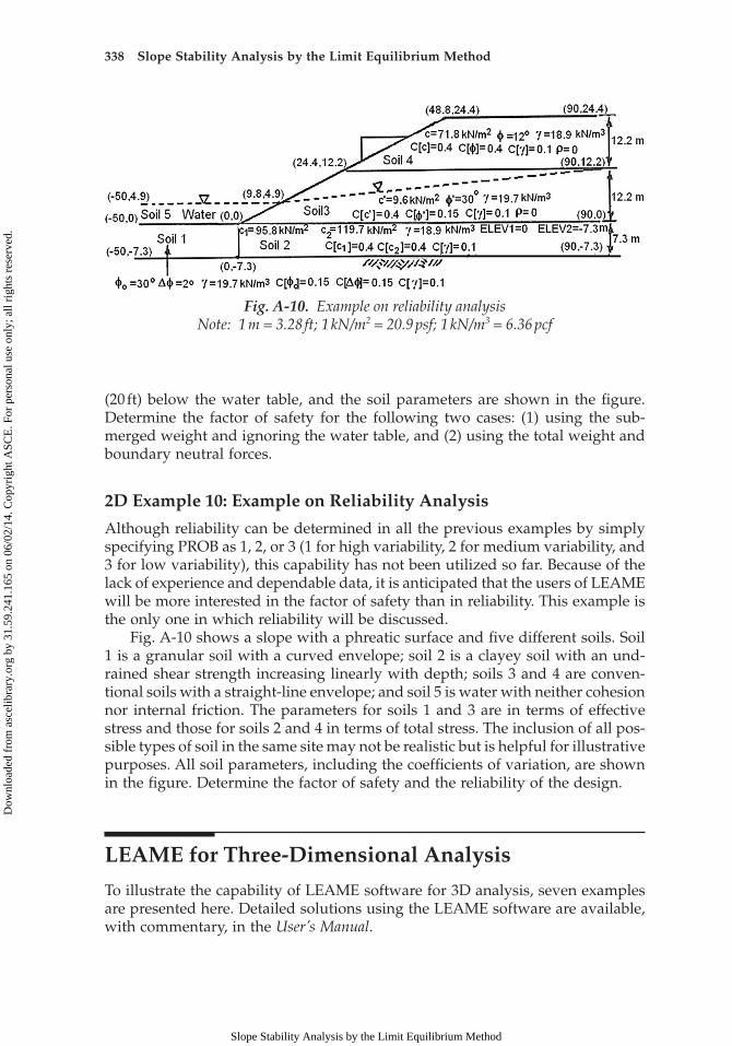
(20 ft) below the water table, and the soil parameters are shown in the figure. Determine the factor of safety for the following two cases: (1) using the sub-merged weight and ignoring the water table, and (2) using the total weight and boundary neutral forces.

2D Example 10: Example on Reliability Analysis

Although reliability can be determined in all the previous examples by simply specifying PROB as 1, 2, or 3 (1 for high variability, 2 for medium variability, and 3 for low variability), this capability has not been utilized so far. Because of the lack of experience and dependable data, it is anticipated that the users of LEAME will be more interested in the factor of safety than in reliability. This example is the only one in which reliability will be discussed.

Fig. A-10 shows a slope with a phreatic surface and five different soils. Soil 1 is a granular soil with a curved envelope; soil 2 is a clayey soil with an und-rained shear strength increasing linearly with depth; soils 3 and 4 are conven-tional soils with a straight-line envelope; and soil 5 is water with neither cohesion nor internal friction. The parameters for soils 1 and 3 are in terms of effective stress and those for soils 2 and 4 in terms of total stress. The inclusion of all pos-sible types of soil in the same site may not be realistic but is helpful for illustrative purposes. All soil parameters, including the coefficients of variation, are shown in the figure. Determine the factor of safety and the reliability of the design.

LEAME for Three-Dimensional Analysis

To illustrate the capability of LEAME software for 3D analysis, seven examples are presented here. Detailed solutions using the LEAME software are available, with commentary, in the User’s Manual.

Fig. A-10. Example on reliability analysisNote: 1 m = 3.28 ft; 1 kN/m2 = 20.9 psf; 1 kN/m3 = 6.36 pcf


Dow

nloa

ded

from

asc

elib

rary

.org

by

31.5

9.24

1.16

5 on

06/

02/1

4. C

opyr

ight

ASC

E. F

or p

erso

nal u

se o

nly;

all

righ

ts r

eser

ved.


3D Example 1: Heavy Surcharge Loads of Limited Length

This example illustrates the application of 3D analysis with ellipsoidal ends to a slope subjected to a heavy load over a limited area. A case in view is the safety to pass extraordinary heavy equipment over an embankment. In 2D analysis, it is assumed that the load and the failure surfaces are infinitely long in the longi-tudinal direction. This assumption is very conservative and may result in an unsatisfactory factor of safety. If the embankment fails under the load, the failure mass must be spoon-shaped with a limited length. Therefore, the use of 3D analysis is more realistic.

Fig. A-11 shows an embankment subjected to two heavy surcharge loads, each 1.2 m (4 ft) wide with a length of 3 m (9.8 ft) and an intensity of 480 kN/m2 (10,000 psf). Soil 1 for the fill has an effective cohesion of 9.6 kN/m2 (200 psf), an effective friction angle of 30°, and a total unit weight of 19.7 kN/m3 (125 pcf). Soils 2 and 3 for the surcharge loads are assumed to have a thickness of 0.3 m (1 ft) and a unit weight of 1,600 kN/m3 (10,000 pcf), which is equivalent to a sur-charge load of 480 kN/m2 (10,000 psf). If the embankment is 18 m (59 ft) long, by the use of LEAME, determine the factors of safety for both 2D and 3D analyses in the same run.

The results of the analysis based on the simplified Bishop method show that the factor of safety is 0.949 for 2D analysis and 1.121 for 3D analysis.

3D Example 2: Failure Surfaces with Planar Ends

If failures occur in a high embankment across a narrow valley with parallel rock banks, two possible types of 3D failures may take place, depending on the inter-facial shear strength between the embankment and the rock bank. If the interfa-cial strength is low, failures will occur along the interface, as well as within the embankment, so the case of 3D analysis with planar ends applies. If the interfa-cial strength is high, failures will not occur along the interface but will be

Fig. A-11. Heavy surcharge loads of limited lengthNote: 1 m = 3.28 ft; 1 kN/m2 = 20.9 psf; 1 kN/m3 = 6.36 pcf


Dow

nloa

ded

from

asc

elib

rary

.org

by

31.5

9.24

1.16

5 on

06/

02/1

4. C

opyr

ight

ASC

E. F

or p

erso

nal u

se o

nly;

all

righ

ts r

eser

ved.


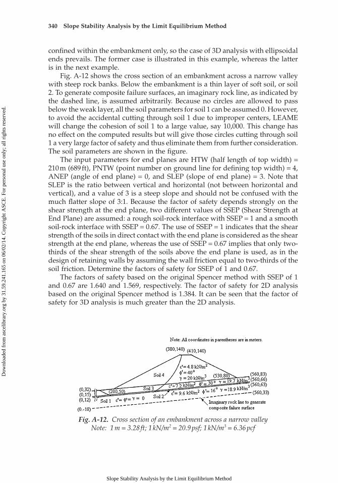
confined within the embankment only, so the case of 3D analysis with ellipsoidal ends prevails. The former case is illustrated in this example, whereas the latter is in the next example.

Fig. A-12 shows the cross section of an embankment across a narrow valley with steep rock banks. Below the embankment is a thin layer of soft soil, or soil 2. To generate composite failure surfaces, an imaginary rock line, as indicated by the dashed line, is assumed arbitrarily. Because no circles are allowed to pass below the weak layer, all the soil parameters for soil 1 can be assumed 0. However, to avoid the accidental cutting through soil 1 due to improper centers, LEAME will change the cohesion of soil 1 to a large value, say 10,000. This change has no effect on the computed results but will give those circles cutting through soil 1 a very large factor of safety and thus eliminate them from further consideration. The soil parameters are shown in the figure.

The input parameters for end planes are HTW (half length of top width) = 210 m (689 ft), PNTW (point number on ground line for defining top width) = 4, ANEP (angle of end plane) = 0, and SLEP (slope of end plane) = 3. Note that SLEP is the ratio between vertical and horizontal (not between horizontal and vertical), and a value of 3 is a steep slope and should not be confused with the much flatter slope of 3:1. Because the factor of safety depends strongly on the shear strength at the end plane, two different values of SSEP (Shear Strength at End Plane) are assumed: a rough soil-rock interface with SSEP = 1 and a smooth soil-rock interface with SSEP = 0.67. The use of SSEP = 1 indicates that the shear strength of the soils in direct contact with the end plane is considered as the shear strength at the end plane, whereas the use of SSEP = 0.67 implies that only two-thirds of the shear strength of the soils above the end plane is used, as in the design of retaining walls by assuming the wall friction equal to two-thirds of the soil friction. Determine the factors of safety for SSEP of 1 and 0.67.

The factors of safety based on the original Spencer method with SSEP of 1 and 0.67 are 1.640 and 1.569, respectively. The factor of safety for 2D analysis based on the original Spencer method is 1.384. It can be seen that the factor of safety for 3D analysis is much greater than the 2D analysis.

Fig. A-12. Cross section of an embankment across a narrow valleyNote: 1 m = 3.28 ft; 1 kN/m2 = 20.9 psf; 1 kN/m3 = 6.36 pcf


Dow

nloa

ded

from

asc

elib

rary

.org

by

31.5

9.24

1.16

5 on

06/

02/1

4. C

opyr

ight

ASC

E. F

or p

erso

nal u

se o

nly;

all

righ

ts r

eser

ved.


3D Example 3: Failure Surfaces with Ellipsoidal Ends

The previous example assumes that the failure surface occurs on the end planes. A question immediately arises: Is the factor of safety based on planar ends lower than that based on ellipsoidal ends? In other words, will the failure occur on the end plane rather than inside the embankment? This example will shed some light on this question.

The cross section and soil parameters used for this example are the same as those in the previous example. If the failure surface is cylindrical with ellipsoidal ends, determine the factor of safety. The result of analysis shows that the factor of safety based on the original Spencer method is 1.430, which is smaller than in the previous example.

3D Example 4: Landfill with Geotextiles and Noncircular Failure Surface

This example illustrates the application of 3D analysis with planar ends to a landfill having a weak layer at the bottom. The use of geosynthetic materials, such as geotextiles, geomembranes, or geosynthetic clay liners at the bottom has posed new problems to the stability of landfills. These materials have a very low friction angle and can cause failures to occur through these weaker materials. When such fills are placed in a hollow with steep slopes on three sides, the factor of safety based on 3D analysis may be smaller than that based on the conven-tional 2D analysis using the most critical cross section at the center. The ability to analyze landfills in three dimensions is an outstanding and important feature of LEAME.

Fig. A-13 shows a landfill with three different materials. The rock toe is con-structed of granular materials with an effective cohesion of 4.8 kN/m2 (100 psf), an effective friction angle of 32°, and a total unit weight of 18.9 kN/m3 (120 pcf). Layers of geotextiles are placed at the bottom of the fill above a clay liner to facilitate construction and provide drainage. To simulate the very small friction angle between geotextiles, a thin layer of material, say 0.1 m (4 in.) thick with a friction angle of only 9° and a unit weight of 17.4 kN/m3 (110 pcf), is placed above the clay liner. Because a weak layer exists at the bottom of the fill, all failure surfaces will lie along the bottom of the weak layer, so all the materials below the weak layer, including the clay liner, are immaterial and need not be consid-ered in the stability analysis. The waste material, or soil 3, above the geotextiles has a cohesion of 9.6 kN/m2 (200 psf), an effective friction angle of 22°, and a total unit weight of 17.4 kN/m3 (110 pcf). The end plane is defined by the following parameters: HTW = 61 m (200 ft), PNTW = 4, SLEP = 0.5, and ANEP = 20°.

Two potential failure surfaces are assumed. The first failure surface assumes that the failure is along the bottom of the fill, starting from (22.9, 38.1) and ending at (201.2, 59.5), as shown in Fig. A-13. The coordinates of the failure surface are the same as those of boundary line 2, so only the shear strength of soil 2 with a friction angle of 9° and the total unit weight of 17.4 kN/m3 (110 pcf) for soils 2 and 3 are used in the analysis.


Dow

nloa

ded

from

asc

elib

rary

.org

by

31.5

9.24

1.16

5 on

06/

02/1

4. C

opyr

ight

ASC

E. F

or p

erso

nal u

se o

nly;

all

righ

ts r

eser

ved.


To be sure that the failure surface does not cut horizontally through the rock toe, a second failure surface is assumed, starting from (7.6, 30.5), passing through (30.5, 30.5), and following boundary line 2 to (201.2, 59.5). Both failure surfaces can be analyzed by LEAME at the same time. The results of the analysis based on the original Spencer method show that failure surface 1 has a safety factor of 1.376, which is more critical than the 1.455 for failure surface 2. The factor of safety for 2D analysis is 1.541, which is much greater than the 3D analysis.

3D Example 5: Landfill with Geotextiles and Composite Failure Surfaces

In the previous example, it is quite possible that the most critical failure surface is a composite surface consisting of a noncircular surface near the toe and a circular surface in the interior, rather than a noncircular surface throughout the entire fill. The factor of safety obtained by the composite failure surface in this example will compare with the noncircular failure surface in the previous example to see which is more critical.

To generate a large number of composite surfaces, an imaginary boundary line 1 is added, and the ground line is extended, as shown by the dashed lines in Fig. A-14. The analysis by LEAME reveals that the minimum factor of safety based on the original Spencer method is 1.373 for composite failure surfaces, which is only slightly smaller than the 1.376 for the noncircular failure surfaces.

Fig. A-13. Landfill with noncircular failure surfacesNote: 1 m = 3.28 ft; 1 kN/m2 = 20.9 psf; 1 kN/m3 = 6.36 pcf

Fig. A-14. Cross section for analyzing composite failure surfacesNote: 1 m = 3.28 ft; 1 kN/m2 = 20.9 psf; 1 kN/m3 = 6.36 pcf


Dow

nloa

ded

from

asc

elib

rary

.org

by

31.5

9.24

1.16

5 on

06/

02/1

4. C

opyr

ight

ASC

E. F

or p

erso

nal u

se o

nly;

all

righ

ts r

eser

ved.


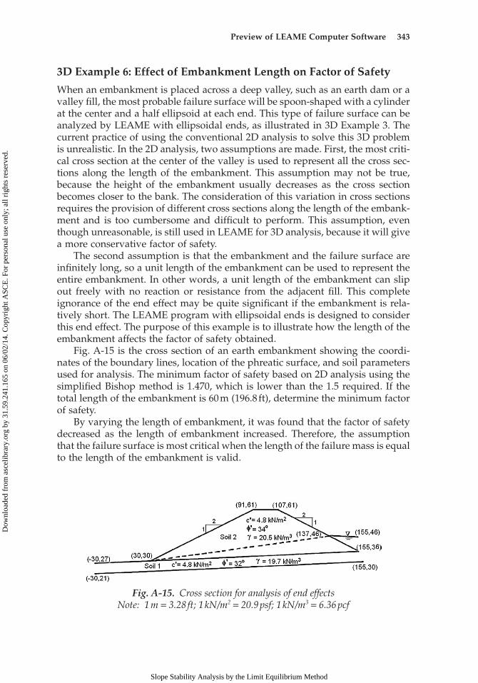
3D Example 6: Effect of Embankment Length on Factor of Safety

When an embankment is placed across a deep valley, such as an earth dam or a valley fill, the most probable failure surface will be spoon-shaped with a cylinder at the center and a half ellipsoid at each end. This type of failure surface can be analyzed by LEAME with ellipsoidal ends, as illustrated in 3D Example 3. The current practice of using the conventional 2D analysis to solve this 3D problem is unrealistic. In the 2D analysis, two assumptions are made. First, the most criti-cal cross section at the center of the valley is used to represent all the cross sec-tions along the length of the embankment. This assumption may not be true, because the height of the embankment usually decreases as the cross section becomes closer to the bank. The consideration of this variation in cross sections requires the provision of different cross sections along the length of the embank-ment and is too cumbersome and difficult to perform. This assumption, even though unreasonable, is still used in LEAME for 3D analysis, because it will give a more conservative factor of safety.

The second assumption is that the embankment and the failure surface are infinitely long, so a unit length of the embankment can be used to represent the entire embankment. In other words, a unit length of the embankment can slip out freely with no reaction or resistance from the adjacent fill. This complete ignorance of the end effect may be quite significant if the embankment is rela-tively short. The LEAME program with ellipsoidal ends is designed to consider this end effect. The purpose of this example is to illustrate how the length of the embankment affects the factor of safety obtained.

Fig. A-15 is the cross section of an earth embankment showing the coordi-nates of the boundary lines, location of the phreatic surface, and soil parameters used for analysis. The minimum factor of safety based on 2D analysis using the simplified Bishop method is 1.470, which is lower than the 1.5 required. If the total length of the embankment is 60 m (196.8 ft), determine the minimum factor of safety.

By varying the length of embankment, it was found that the factor of safety decreased as the length of embankment increased. Therefore, the assumption that the failure surface is most critical when the length of the failure mass is equal to the length of the embankment is valid.

Fig. A-15. Cross section for analysis of end effectsNote: 1 m = 3.28 ft; 1 kN/m2 = 20.9 psf; 1 kN/m3 = 6.36 pcf


Dow

nloa

ded

from

asc

elib

rary

.org

by

31.5

9.24

1.16

5 on

06/

02/1

4. C

opyr

ight

ASC

E. F

or p

erso

nal u

se o

nly;

all

righ

ts r

eser

ved.


3D Example 7: Effect of Bench Length on Factor of Safety

In 2D analysis, not only the failure surface but also the loading must be infinitely long. If a load is applied over a limited area, the 3D analysis with ellipsoidal ends can be used, as illustrated in 3D Example 1. The same principle can be applied to a short section of steep slope changing gradually to a much flatter slope. The section of steep slope can be considered as a heavy load with a HCL (half cylindrical length) equal to the half length of the steeper section. However, there are two major differences between 3D Example 1 and this case: (1) The half length of the failure mass (HLFM) is defined clearly as the half length of the embankment in 3D Example 1 but not in this case. Because the flatter slope is very stable with a high factor of safety, HLFM should be confined within the transitional and steep sections and not extended into the flatter section; and (2) In 3D Example 1, the cross section is the same throughout the embankment, whereas in this example the half ellipsoid is located in the transitional section with a gradually decreasing slope, so the assumption of the same steep slope for the transitional section is on the safe side with a lower factor of safety.

This method can be applied to the stability analysis of bench fills. In surface mining, a cut is made on a hillside to expose the coal seam, resulting in a bench and a highwall. The Surface Mining Control and Reclamation Act of 1977 requires the return of disturbed land to its original contours. Therefore, the bench created by surface mining must be backfilled to the original slope. If the original slope is quite steep, it may be difficult to achieve the required factor of safety. The factor of safety can be increased by 3D analysis.

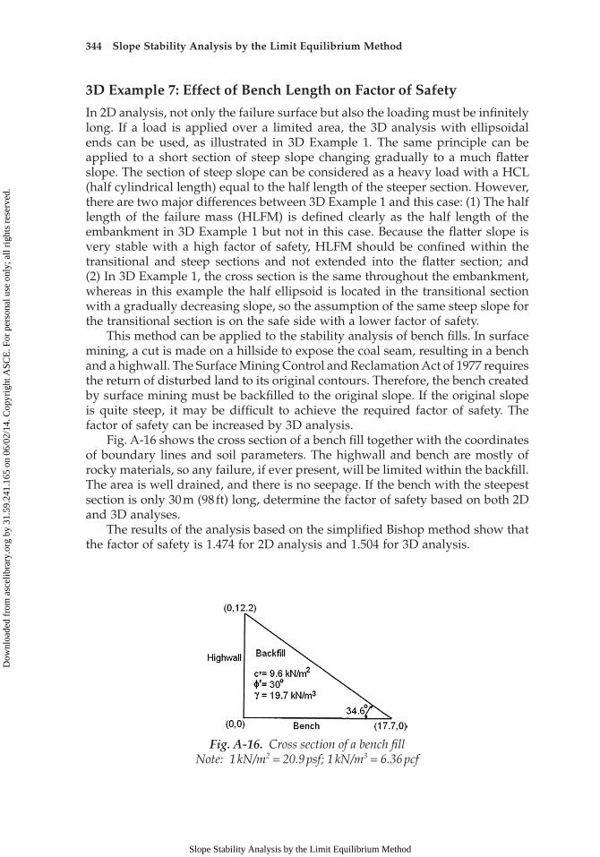
Fig. A-16 shows the cross section of a bench fill together with the coordinates of boundary lines and soil parameters. The highwall and bench are mostly of rocky materials, so any failure, if ever present, will be limited within the backfill. The area is well drained, and there is no seepage. If the bench with the steepest section is only 30 m (98 ft) long, determine the factor of safety based on both 2D and 3D analyses.

The results of the analysis based on the simplified Bishop method show that the factor of safety is 1.474 for 2D analysis and 1.504 for 3D analysis.

Fig. A-16. Cross section of a bench fillNote: 1 kN/m2 = 20.9 psf; 1 kN/m3 = 6.36 pcf


Dow

nloa

ded

from

asc

elib

rary

.org

by

31.5

9.24

1.16

5 on

06/

02/1

4. C

opyr

ight

ASC

E. F

or p

erso

nal u

se o

nly;

all

righ

ts r

eser

ved.


Applications for Surface Mining

As mentioned in the Preface to this book, the original REAME software (Rota-tional Equilibrium Analysis of Multilayered Embankments) was developed in response to the Surface Mining Control and Reclamation Act of 1977, which requires the stability analysis of spoil banks, hollow fills, and refuse dams created by surface mining. In Chapter 4 of the LEAME User’s Manual, 10 cases involving various methods of spoil and waste disposal from surface mining are presented to illustrate the practical applications of LEAME. Data files for these cases are included with the software and can be used to run LEAME and obtain the printed results. These examples are real cases that were analyzed by REAME and submitted to the regulatory agencies for the application of mining permits. Because the LEAME presented in this book is quite different from the original REAME, the stability analyses reported herein are not exactly the same as those in the original reports. However, the general procedures and conclusions are about the same.


Dow

nloa

ded

from

asc

elib

rary

.org

by

31.5

9.24

1.16

5 on

06/

02/1

4. C

opyr

ight

ASC

E. F

or p

erso

nal u

se o

nly;

all

righ

ts r

eser

ved.

9780784412886.bm01

Documents