978-1-58503-485-7 -- introduction to autocad 2008 for civil

Introduction to AutoCAD 2008 for

Civil Engineering Applications

Learning to use AutoCAD for Civil Engineering projects

Contours

Siteplan

Drainage Basin

Floodplain

Transportation

Earthwork

Nighat Yasmin Clemson University

SDC

Schroff Development Corporation www.schroff.com

Better Textbooks. Lower Prices.

PUBLICATIONS

Copyrighted Material

Copyrighted

Material


Copyrighted

Material

Contours 245

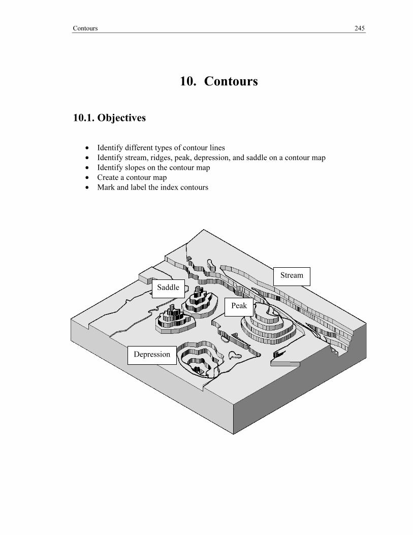
10. Contours

10.1. Objectives

• Identify different types of contour lines

• Identify stream, ridges, peak, depression, and saddle on a contour map

• Identify slopes on the contour map

• Create a contour map

• Mark and label the index contours

Depression

Peak

Saddle

Stream


Copyrighted

Material


Copyrighted

Material

246 Introduction to AutoCAD for Civil Engineering Applications

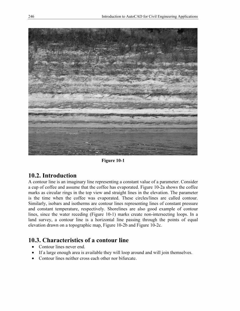
Figure 10-1

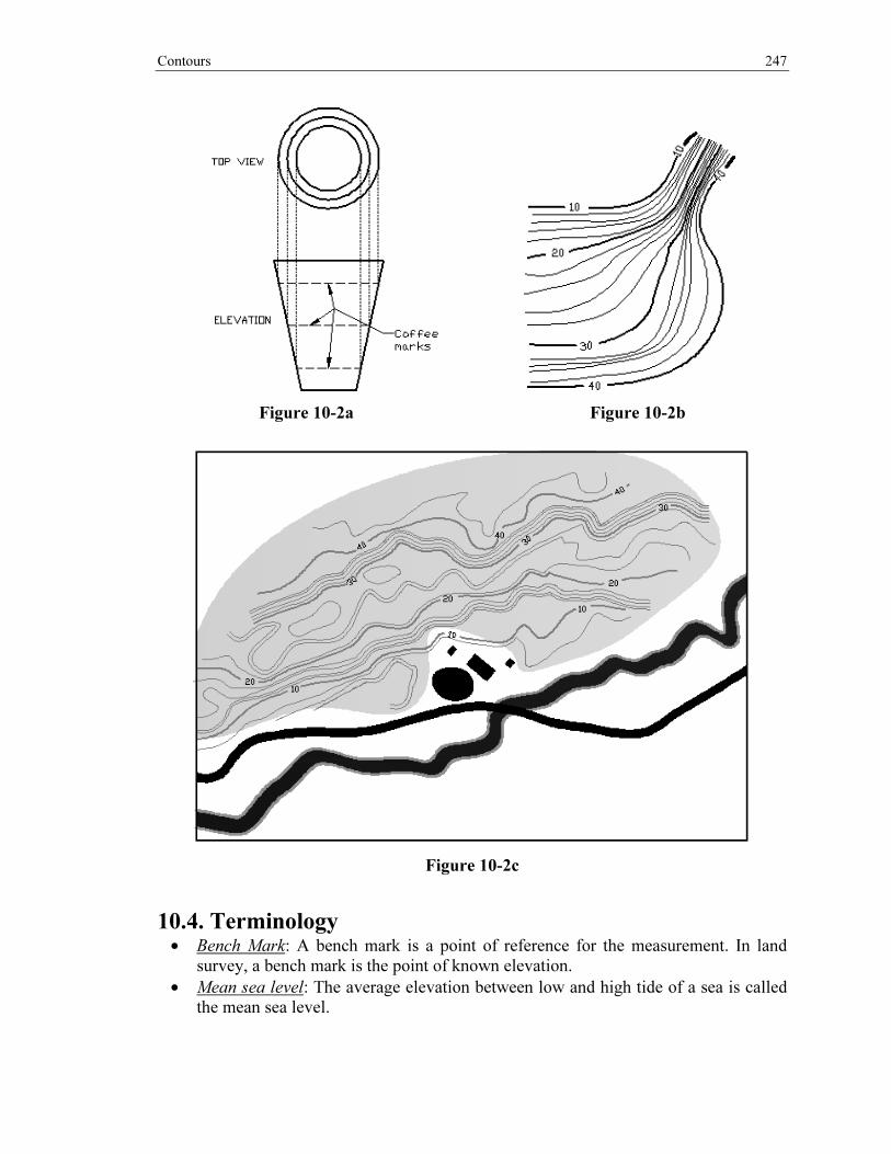
10.2. Introduction A contour line is an imaginary line representing a constant value of a parameter. Consider a cup of coffee and assume that the coffee has evaporated. Figure 10-2a shows the coffee marks as circular rings in the top view and straight lines in the elevation. The parameter is the time when the coffee was evaporated. These circles/lines are called contour. Similarly, isobars and isotherms are contour lines representing lines of constant pressure and constant temperature, respectively. Shorelines are also good example of contour lines, since the water receding (Figure 10-1) marks create non-intersecting loops. In a land survey, a contour line is a horizontal line passing through the points of equal elevation drawn on a topographic map, Figure 10-2b and Figure 10-2c.

10.3. Characteristics of a contour line • Contour lines never end.

• If a large enough area is available they will loop around and will join themselves.

• Contour lines neither cross each other nor bifurcate.


Copyrighted

Material


Copyrighted

Material

Contours 247

Figure 10-2a Figure 10-2b

Figure 10-2c

10.4. Terminology • Bench Mark: A bench mark is a point of reference for the measurement. In land

survey, a bench mark is the point of known elevation.

• Mean sea level: The average elevation between low and high tide of a sea is called the mean sea level.


Copyrighted

Material


Copyrighted

Material


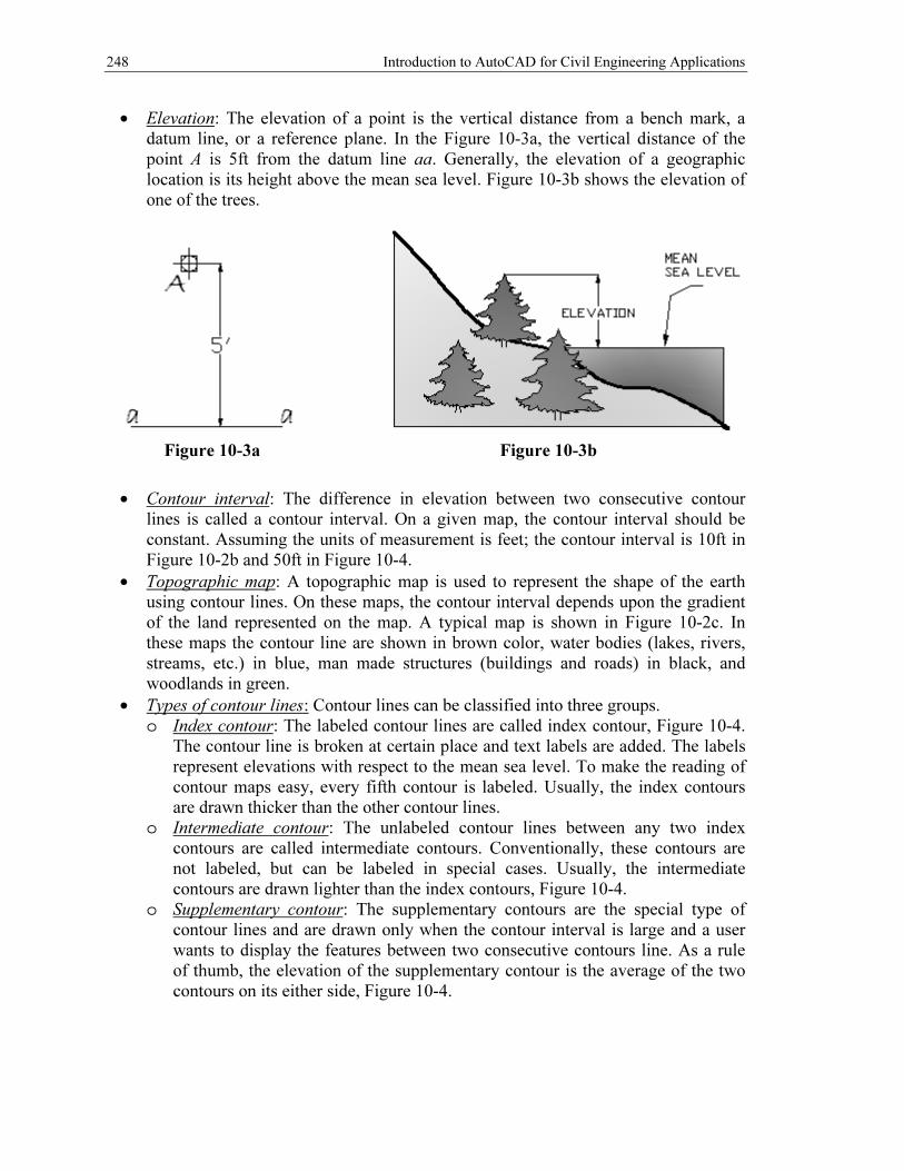
• Elevation: The elevation of a point is the vertical distance from a bench mark, a datum line, or a reference plane. In the Figure 10-3a, the vertical distance of the point A is 5ft from the datum line aa. Generally, the elevation of a geographic location is its height above the mean sea level. Figure 10-3b shows the elevation of one of the trees.


• Contour interval: The difference in elevation between two consecutive contour lines is called a contour interval. On a given map, the contour interval should be constant. Assuming the units of measurement is feet; the contour interval is 10ft in Figure 10-2b and 50ft in Figure 10-4.

• Topographic map: A topographic map is used to represent the shape of the earth using contour lines. On these maps, the contour interval depends upon the gradient of the land represented on the map. A typical map is shown in Figure 10-2c. In these maps the contour line are shown in brown color, water bodies (lakes, rivers, streams, etc.) in blue, man made structures (buildings and roads) in black, and woodlands in green.

• Types of contour lines: Contour lines can be classified into three groups. o Index contour: The labeled contour lines are called index contour, Figure 10-4.

The contour line is broken at certain place and text labels are added. The labels represent elevations with respect to the mean sea level. To make the reading of contour maps easy, every fifth contour is labeled. Usually, the index contours are drawn thicker than the other contour lines.

o Intermediate contour: The unlabeled contour lines between any two index contours are called intermediate contours. Conventionally, these contours are not labeled, but can be labeled in special cases. Usually, the intermediate contours are drawn lighter than the index contours, Figure 10-4.

o Supplementary contour: The supplementary contours are the special type of contour lines and are drawn only when the contour interval is large and a user wants to display the features between two consecutive contours line. As a rule of thumb, the elevation of the supplementary contour is the average of the two contours on its either side, Figure 10-4.


Copyrighted

Material


Copyrighted

Material

Contours 249

Figure 10-4

• Peak: The peak of a hill or mountain is shown by the circular contour lines of decreasing diameters and increasing elevation. Figure 10-5a and Figure 10-5b shows the contour map and the accompanying peak, respectively.


• Depression: The bottom of a depression (hole or excavation without any drainage outlets) is shown by the circular contour lines of decreasing diameters and decreasing elevation. Figure 10-6a and Figure 10-6b shows the contour map and the accompanying depression, respectively. The innermost circle is marked with small lines on the inside.


Copyrighted

Material


Copyrighted

Material



• Saddle: Two peaks side by side form a saddle. Figure 10-7a and Figure 10-7b shows the contour map and the accompanying depression, respectively.


• Slope verses space: Closely spaced contour lines represent steep slope and widely spaced contour lines represent mild slope, Figure 10-8.

Figure 10-8


Copyrighted

Material


Copyrighted

Material

Contours 251

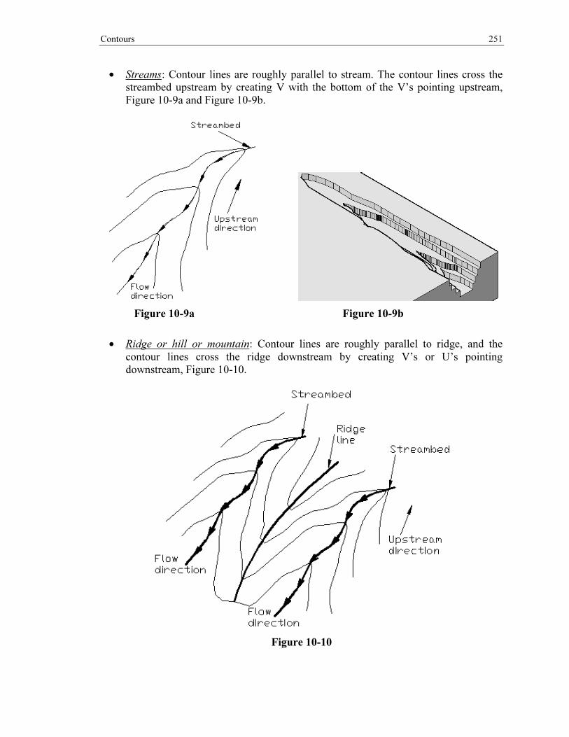
• Streams: Contour lines are roughly parallel to stream. The contour lines cross the streambed upstream by creating V with the bottom of the V’s pointing upstream, Figure 10-9a and Figure 10-9b.


• Ridge or hill or mountain: Contour lines are roughly parallel to ridge, and the contour lines cross the ridge downstream by creating V’s or U’s pointing downstream, Figure 10-10.

Figure 10-10


Copyrighted

Material


Copyrighted

Material


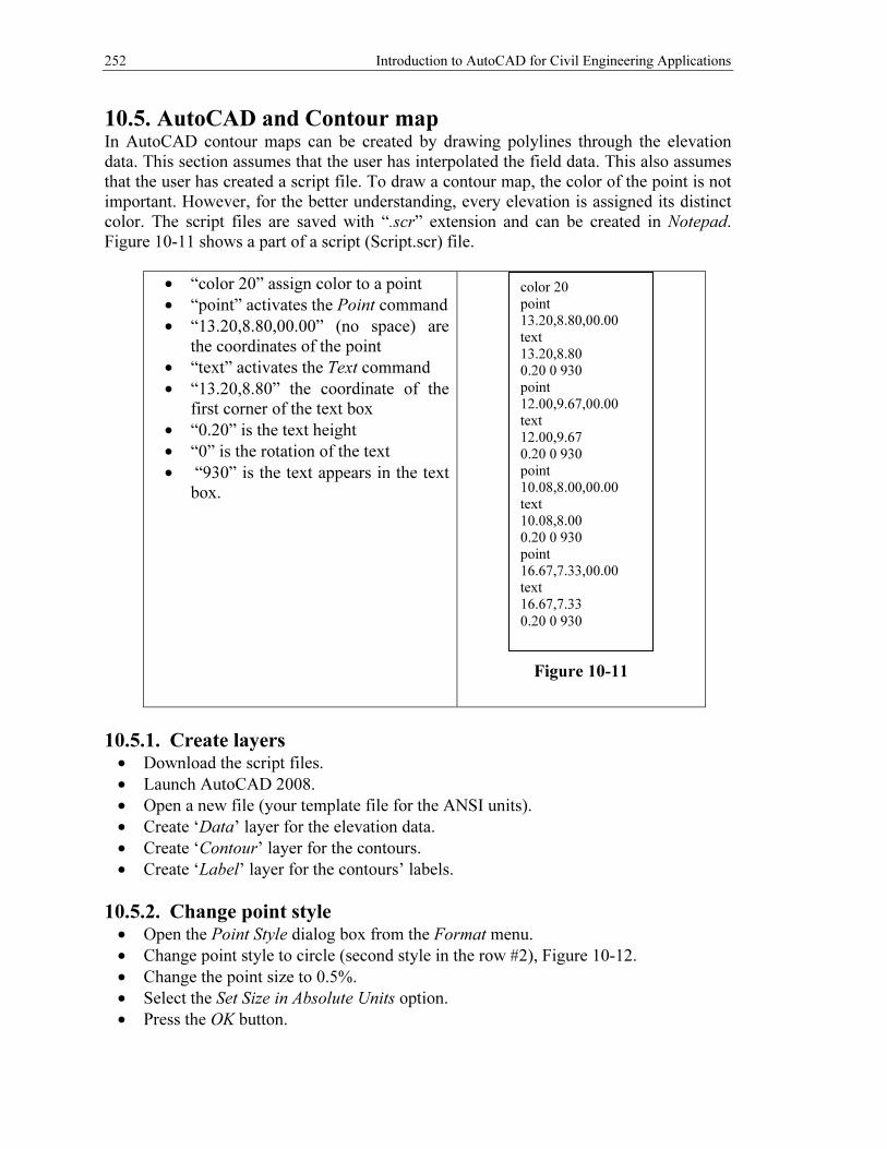
10.5. AutoCAD and Contour map In AutoCAD contour maps can be created by drawing polylines through the elevation data. This section assumes that the user has interpolated the field data. This also assumes that the user has created a script file. To draw a contour map, the color of the point is not important. However, for the better understanding, every elevation is assigned its distinct color. The script files are saved with “.scr” extension and can be created in Notepad. Figure 10-11 shows a part of a script (Script.scr) file.

• “color 20” assign color to a point

• “point” activates the Point command

• “13.20,8.80,00.00” (no space) are the coordinates of the point

• “text” activates the Text command

• “13.20,8.80” the coordinate of the first corner of the text box

• “0.20” is the text height

• “0” is the rotation of the text

• “930” is the text appears in the text box.

Figure 10-11

10.5.1. Create layers • Download the script files.

• Launch AutoCAD 2008.

• Open a new file (your template file for the ANSI units).

• Create ‘Data’ layer for the elevation data.

• Create ‘Contour’ layer for the contours.

• Create ‘Label’ layer for the contours’ labels.

10.5.2. Change point style • Open the Point Style dialog box from the Format menu.

• Change point style to circle (second style in the row #2), Figure 10-12.

• Change the point size to 0.5%.

• Select the Set Size in Absolute Units option.

• Press the OK button.

color 20

point

13.20,8.80,00.00

text

13.20,8.80

0.20 0 930

point

12.00,9.67,00.00

text

12.00,9.67

0.20 0 930

point

10.08,8.00,00.00

text

10.08,8.00

0.20 0 930

point

16.67,7.33,00.00

text

16.67,7.33

0.20 0 930


Copyrighted

Material


Copyrighted

Material

Contours 253

Figure 10-12

10.5.3. Read the script files • Make the Data layer as the current layer.

• Read the script file: o Activate the script command.

� Menu method: Select the Tool dropdown menu and click on the Run Script

option. � Command line method: Type “script”, “Script”, or “SCRIPT” on the

command line and press the Enter key.

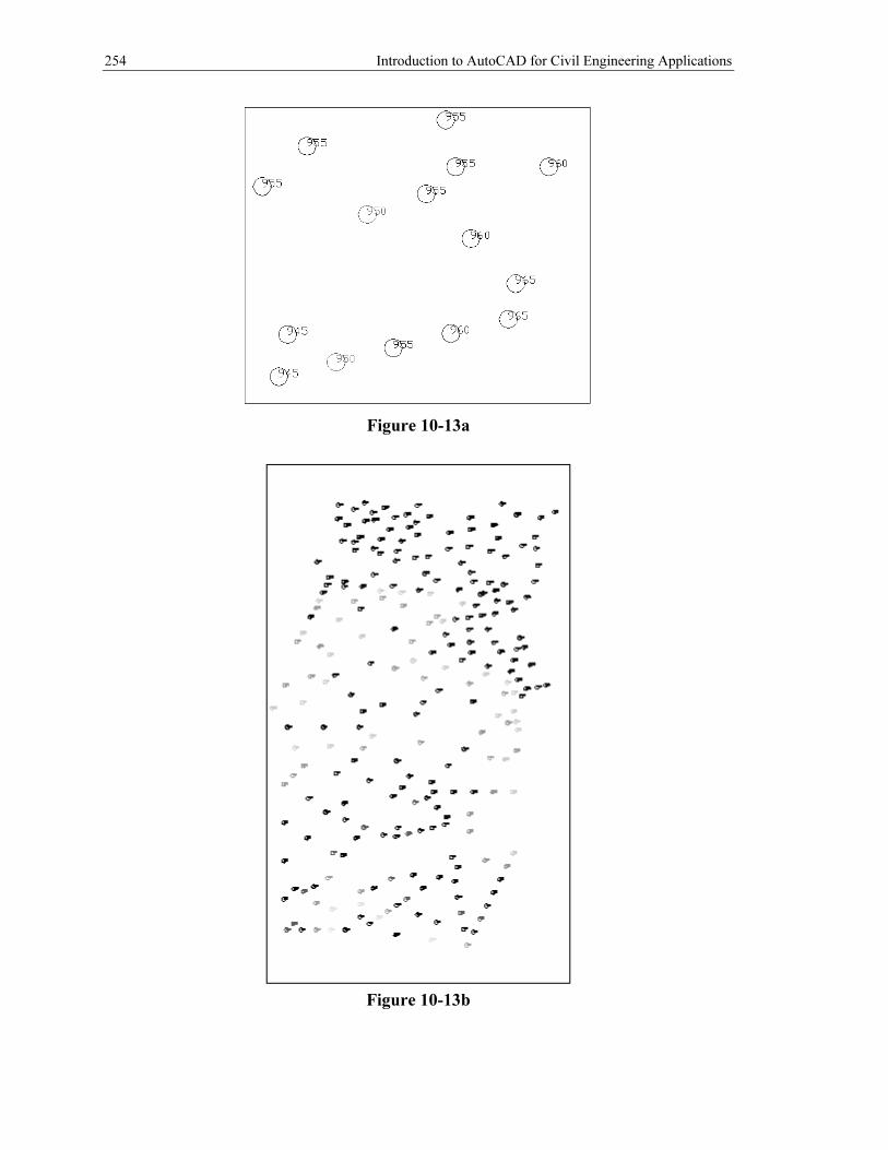
• Figure 10-13a shows the close-up of the selected elevation data points.

• The complete elevation data is shown in Figure 10-13b.


Copyrighted

Material


Copyrighted

Material


Figure 10-13a

Figure 10-13b


Copyrighted

Material


Copyrighted

Material

Contours 255

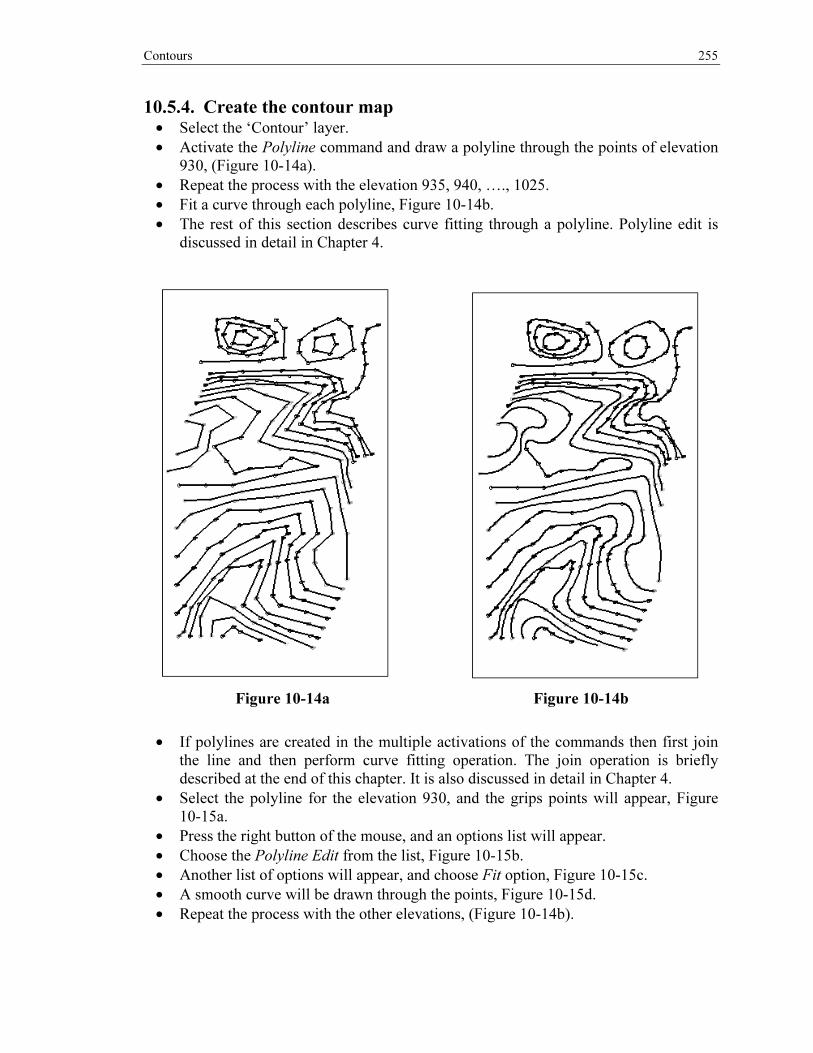
10.5.4. Create the contour map • Select the ‘Contour’ layer.

• Activate the Polyline command and draw a polyline through the points of elevation 930, (Figure 10-14a).

• Repeat the process with the elevation 935, 940, …., 1025.

• Fit a curve through each polyline, Figure 10-14b.

• The rest of this section describes curve fitting through a polyline. Polyline edit is discussed in detail in Chapter 4.


• If polylines are created in the multiple activations of the commands then first join the line and then perform curve fitting operation. The join operation is briefly described at the end of this chapter. It is also discussed in detail in Chapter 4.

• Select the polyline for the elevation 930, and the grips points will appear, Figure 10-15a.

• Press the right button of the mouse, and an options list will appear.

• Choose the Polyline Edit from the list, Figure 10-15b.

• Another list of options will appear, and choose Fit option, Figure 10-15c.

• A smooth curve will be drawn through the points, Figure 10-15d.

• Repeat the process with the other elevations, (Figure 10-14b).


Copyrighted

Material


Copyrighted

Material


Figure 10-15a

Figure 10-15b

Figure 10-15c

Figure 10-15d

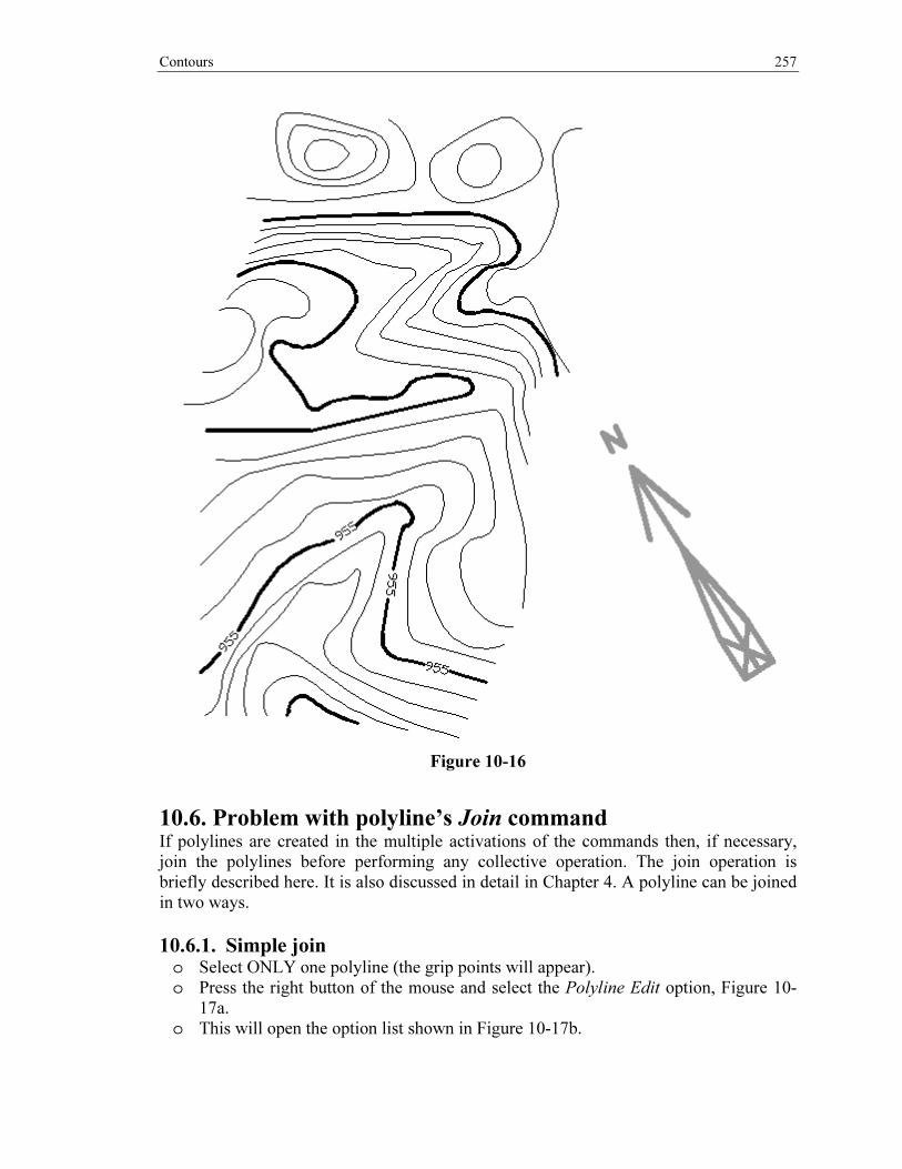
10.5.5. Add the labels to the index contours • If polylines are created in the multiple activations of the commands, then first join

the line, and then perform marking and labeling operation. The join operation is briefly described at the end of this chapter, and is discussed in detail in Chapter 4.

• Mark the index contours (that is, increase the lineweight for the index contours).

• Use the Text command from the Draw toolbar to create the text of a label. The text should be perpendicular to the polyline. If necessary, use the Rotate command from the Modify toolbar to rotate the text.

• Use the Break command from the Modify toolbar to break the polyline. The Break command is discussed in the next section.

• The Figure 10-16 shows a contour map with only one labeled index contours.

• Similarly add labels to the other contours.

• Finally, add the north direction to the map, Figure 10-16.


Copyrighted

Material


Copyrighted

Material

Contours 257

Figure 10-16

10.6. Problem with polyline’s Join command If polylines are created in the multiple activations of the commands then, if necessary, join the polylines before performing any collective operation. The join operation is briefly described here. It is also discussed in detail in Chapter 4. A polyline can be joined in two ways.

10.6.1. Simple join o Select ONLY one polyline (the grip points will appear). o Press the right button of the mouse and select the Polyline Edit option, Figure 10-

17a. o This will open the option list shown in Figure 10-17b.


Copyrighted

Material


Copyrighted

Material


o Select the Join option by clicking the left button of the mouse. This will close the option selection list and the user is allowed to select the polylines to be joined.

o Click with the left button of the mouse Figure 10-17c and press the Enter key TWICE.

o The multiple polylines are converted to a single polyline. o The result is shown in Figure 10-17d.

Figure 10-17a

Figure 10-17b

Figure 10-17c

Figure 10-17d

10.6.2. Join by setting the fuzz distance • Open Modify II toolbar (it is a toolbar to edit polylines).

• Choose Polyline Edit tool (third from the left end of the bar).

• Press the down arrow and choose the Multiple’s option.

• Select all four lines and press the enter key.

• Select the Join option.

• Press the down arrow and choose Both option.

• Specify the Fuzz distance to be 20 (that is, if the space between the two lines is less then or equal to this number, the lines will be connected).

• Press the Enter key twice.

• The multiple polylines are converted to a single polyline.

978-1-58503-485-7 -- introduction to autocad 2008 for civil

Documents