9.1 - 1 copyright © 2010, 2007, 2004 pearson education, inc. section 9-2 inferences about two...

Copyright © 2010, 2007, 2004 Pearson Education, Inc. 9.1 - 1

Section 9-2 Inferences About Two

Proportions


Key Concept

In this section we present methods for (1) testing a claim made about the two population proportions and (2) constructing a confidence interval estimate of the difference between the two population proportions. This section is based on proportions, but we can use the same methods for dealing with probabilities or the decimal equivalents of percentages.


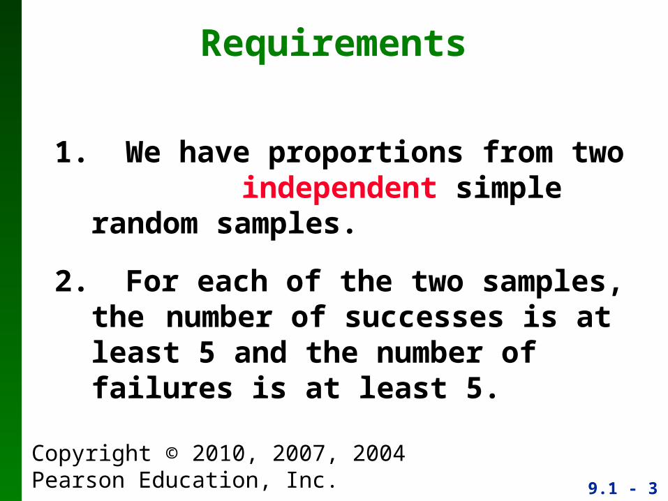
Requirements

1. We have proportions from two independent simple random samples.

2. For each of the two samples, the number of successes is at least 5 and the number of failures is at least 5.


Test Statistic for Two Proportions - cont

P-value: Use Table A-2. (Use the computed value of the test statistic z and find its P-value by following the procedure summarized by Figure 8-5 in the text.)

Critical values: Use Table A-2. (Based on the significance level , find critical values by using the procedures introduced in Section 8-2 in the text.)

a


Example:

The table below lists results from a simple random sample of front-seat occupants involved in car crashes. Use a 0.05 significance level to test the claim that the fatality rate of occupants is lower for those in cars equipped with airbags.


Example:

Requirements are satisfied: two simple random samples, two samples are independent; Each has at least 5 successes and 5 failures (11,500, 41; 9801, 52).Use the P-value method.

Step 1: Express the claim as p1 < p2 .

Step 2: If p1 < p2 is false, then p1 ≥ p2 .

Step 3: p1 < p2 does not contain equality so it is the alternative hypothesis. The null hypothesis is the statement of equality.


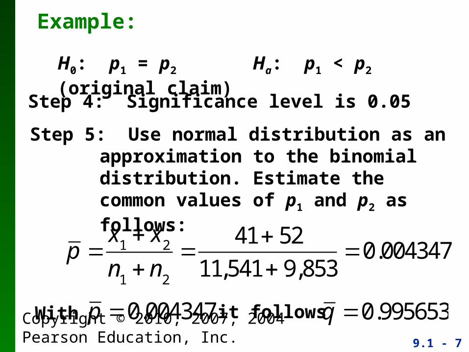
Example:

H0: p1 = p2 Ha: p1 < p2 (original claim)

Step 4: Significance level is 0.05

Step 5: Use normal distribution as an approximation to the binomial distribution. Estimate the common values of p1 and p2 as follows:

p

x1 x

2

n1 n

2

41 52

11,541 9,8530.004347

With p 0.004347 it follows q 0.995653


Example:Step 6: Find the value of the test statistic.

41 520

11 541 9 853

0 004347 0 995653 0 004347 0 995653

11 541 9 853

, ,

. . . .

, ,

z 1.91

z p̂1 p̂2 p1 p2

pqn1

pqn2


Example:

Left-tailed test. Area to left of z = –1.91 is 0.0281 (Table A-2), so the P-value is 0.0281.


Example:

Step 7: Because the P-value of 0.0281 is less than the significance level of= 0.05, we reject the null hypothesis of p1 = p2.

Because we reject the null hypothesis, we conclude that there is sufficient evidence to support the claim that the proportion of accident fatalities for occupants in cars with airbags is less than the proportion of fatalities for occupants in cars without airbags. Based on these results, it appears that airbags are effective in saving lives.


Example: Using the Traditional Method

distribution, we refer to Table A-2 and find that an area of = 0.05 in the left tail corresponds to the critical value of z = –1.645. The test statistic of does fall in the critical region bounded by the critical value of z = –1.645.We again reject the null hypothesis.

With a significance level of = 0.05 in a left- tailed test based on the normal

a


Caution

When testing a claim about two population proportions, the P-value method and the traditional method are equivalent, but they are not equivalent to the confidence interval method. If you want to test a claim about two population proportions, use the P-value method or traditional method; if you want to estimate the difference between two population proportions, use a confidence interval.


Example:

Use the sample data given in the preceding Example to construct a 90% confidence interval estimate of the difference between the two population proportions. (As shown in Table 8-2 on page 406, the confidence level of 90% is comparable to the significance level of = 0.05 used in the preceding left-tailed hypothesis test.) What does the result suggest about the effectiveness of airbags in an accident?

a


Example:Requirements are satisfied as we saw in the preceding example.

90% confidence interval: zα/2 = 1.645Calculate the margin of error,

1.645

4111,541

11,50011,541

11,541

529,853

98019,853

9,853

0.001507

E z 2

p̂1q̂1

n1

p̂2q̂2

n2


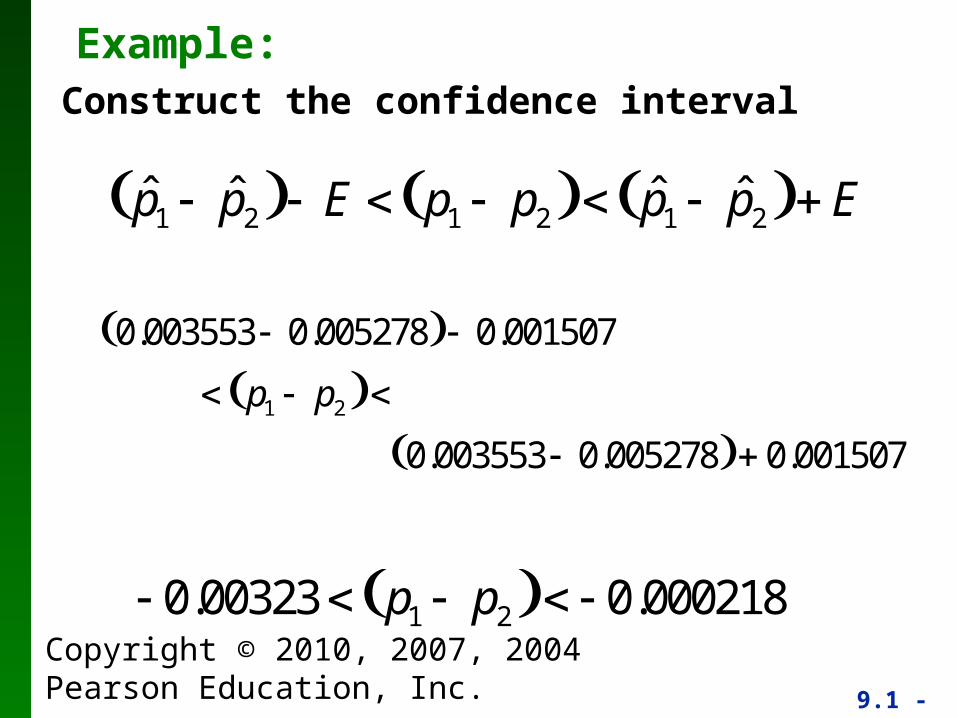
Example:Construct the confidence interval

0.003553 0.005278 0.001507

p1 p2 0.003553 0.005278 0.001507

p̂1 p̂2 E p1 p2 p̂1 p̂2 E

0.00323 p1 p2 0.000218


Example:

The confidence interval limits do not contain 0, implying that there is a significant difference between the two proportions. The confidence interval suggests that the fatality rate is lower for occupants in cars with air bags than for occupants in cars without air bags. The confidence interval also provides an estimate of the amount of the difference between the two fatality rates.


Why Do the Procedures of This Section Work?

The distribution of can be approximated by a normal distribution with mean p1, standard deviation and variance p1q1/n1.

The difference can be approximated by a normal distribution with mean p1 – p2 and variance

p1q

1n

1,

1 2ˆ ˆp p

p̂1

1 21 2

2 2 2 1 1 2 2ˆ ˆˆ ˆ

1 2p pp p

p q p q

n n

The variance of the differences between two independent random variables is the sum of their individual variances.



The preceding variance leads to

1 2

1 1 2 2ˆ ˆ

1 2p p

p q p q

n n

We now know that the distribution of p1 – p2 is approximately normal, with mean p1 – p2 and standard deviation as shown above, so the z test statistic has the form given earlier.



When constructing the confidence interval estimate of the difference between two proportions, we don’t assume that the two proportions are equal, and we estimate the standard deviation as

p̂1q̂1

n1

p̂2q̂2

n2



In the test statistic

use the positive and negative values of z (for two tails) and solve for p1 – p2. The results are the limits of the confidence interval given earlier.

z p̂1 p̂2 p1 p2

p̂1q̂1

n1

p̂2q̂2

n2


Section 9-3 Inferences About Two Means: Independent

Samples


Key Concept

This section presents methods for using sample data from two independent samples to test hypotheses made about two population means or to construct confidence interval estimates of the difference between two population means.


Key Concept

In Part 1 we discuss situations in which the standard deviations of the two populations are unknown and are not assumed to be equal. In Part 2 we discuss two other situations: (1) The two population standard deviations are both known; (2) the two population standard deviations are unknown but are assumed to be equal. Because is typically unknown in real situations, most attention should be given to the methods described in Part 1.


Part 1: Independent Samples with σ1 and σ2 Unknown and Not

Assumed Equal


DefinitionsTwo samples are independent if the sample values selected from one population are not related to or somehow paired or matched with the sample values from the other population.

Two samples are dependent if the sample values are paired. (That is, each pair of sample values consists of two measurements from the same subject (such as before/after data), or each pair of sample values consists of matched pairs (such as husband/wife data), where the matching is based on some inherent relationship.)


Hypothesis Test for Two Means: Independent Samples

t x

1 x

2 1

2 s

12

n1

s

22

n2


Degrees of freedom: In this book we use this simple and conservative estimate: df = smaller of n1 – 1 and n2 – 1.

P-values: Refer to Table A-3. Use the procedure summarized in Figure 8-5.

Critical values: Refer to Table A-3.

Hypothesis Test - cont

Test Statistic for Two Means: Independent Samples


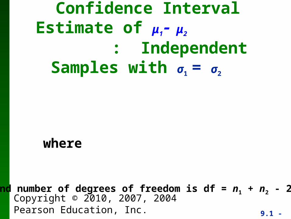
Confidence Interval Estimate ofμ1μ2: Independent Samples

where df = smaller n1 – 1 and n2 – 1

where

1 2 1 2 1 2( ) ( ) ( )x x E x x E

2 21 2

21 2

s sE t

n n


Caution

Before conducting a hypothesis test, consider the context of the data, the source of the data, the sampling method, and explore the data with graphs and descriptive statistics. Be sure to verify that the requirements are satisfied.


Example:A headline in USA Today proclaimed that “Men, women are equal talkers.” That headline referred to a study of the numbers of words that samples of men and women spoke in a day. Given below are the results from the study. Use a 0.05 significance level to test the claim that men and women speak the same mean number of words in a day. Does there appear to be a difference?


Example:Requirements are satisfied: two population standard deviations are not known and not assumed to be equal, independent samples, simple random samples, both samples are large.

Step 1: Express claim as μ1μ2 .Step 2: If original claim is false, then

μ1μ2 .Step 3: Alternative hypothesis does not

contain equality, null hypothesis does.

(original claim) H0μ1

μ2

HAμ1

μ2


Example:Step 4: Significance level is 0.05

Step 5: Use a t distribution

Step 6: Calculate the test statistic

t x

1 x

2 1

2 s

12

n1

s

22

n2

15,668.5 16,215.0 0

8632.52

186

7301.22

210

0.676


Example:Use Table A-3: area in two tails is 0.05, df = 185, which is not in the table, the closest value is

1.972t 1.972


Example:Step 7: Because the test statistic does not fall

within the critical region, fail to reject the null hypothesis:

There is not sufficient evidence to warrant rejection of the claim that men and women speak the same mean number of words in a day. There does not appear to be a significant difference between the two means.

H0μ1

μ2


Example:

Using the sample data given in the previous Example, construct a 95% confidence interval estimate of the difference between the mean number of words spoken by men and the mean number of words spoken by women.


Example:Requirements are satisfied as it is the same data as the previous example.

Find the margin of Error, E; use t/2 = 1.972

Construct the confidence interval use E = 1595.4 and

E t 2

s12

n1

s

22

n2

1.9728632.52

186

7301.22

2101595.4

x1 x

2 E 1

2 x1 x

2 E

2141.9 1

2 1048.9

x115,668.5 and x

216,215.0.


Assume that σ1 = σ2 and Pool the Sample Variances.


Requirements

1. The two population standard deviations are not known, but they are assumed to be

equal. That is σ1 = σ2 .

2. The two samples are independent.

3. Both samples are simple random samples.

4. Either or both of these conditions are satisfied: The two sample sizes are both large (with n1 > 30 and n2 > 30) or both samples come from populations having normal distributions.


Hypothesis Test Statistic for Two Means: Independent Samples and

σ1 = σ2

Where

and the number of degrees of freedom is df = n1 + n2 - 2

2 2

1 2

1 2 1 2( ) ( )

p ps S

n n

x xt

2 22 1 1 2 2

1 2

( 1) ( 1)

( 1) ( 1)p

n s n ss

n n


Confidence Interval Estimate of μ1μ2

: Independent Samples with σ1 = σ2

where

and number of degrees of freedom is df = n1 + n2 - 2

1 2 1 2 1 2( ) ( ) ( )x x E x x E

2 2

21 2

p ps sE t

n n


Strategy

Unless instructed otherwise, use the following strategy:

Assume that σ1 and σ2 are unknown, do not

assume that σ1 = σ2 , and use the test statistic and confidence interval given in Part 1 of this section. (See Figure 9-3.)


Methods for Inferences About Two Independent Means

Figure 9-3


Section 9-4 Inferences from Matched

Pairs


Key Concept

In this section we develop methods for testing hypotheses and constructing confidence intervals involving the mean of the differences of the values from two dependent populations.

With dependent samples, there is some relationship whereby each value in one sample is paired with a corresponding value in the other sample.


Key Concept

Because the hypothesis test and confidence interval use the same distribution and standard error, they are equivalent in the sense that they result in the same conclusions. Consequently, the null hypothesis that the mean difference equals 0 can be tested by determining whether the confidence interval includes 0. There are no exact procedures for dealing with dependent samples, but the t distribution serves as a reasonably good approximation, so the following methods are commonly used.


Requirements

1. The sample data are dependent.

2. The samples are simple random samples.

3. Either or both of these conditions is satisfied: The number of pairs of sample data is large (n > 30) or the pairs of values have differences that are from a population having a distribution that is approximately normal.


Example:

Data Set 3 in Appendix B includes measured weights of college students in September and April of their freshman year. Table 9-1 lists a small portion of those sample values. (Here we use only a small portion of the available data so that we can better illustrate the method of hypothesis testing.) Use the sample data in Table 9-1 with a 0.05 significance level to test the claim that for the population of students, the mean change in weight from September to April is equal to 0 kg.


Example:

Requirements are satisfied: samples are dependent, values paired from each student; although a volunteer study, we’ll proceed as if simple random sample and deal with this in the interpretation; STATDISK displays a histogram that is approximately normal


Example:

Weight gained = April weight – Sept. weight

μdenotes the mean of the “April – Sept.”

differences in weight; the claim is μ kg

Step 1: claim is μ kg

Step 2: If original claim is not true, we have

μ Step 3: H0μ original claim Step 4: significance level is = 0.05

Step 5: use the student t distribution

a


Example:

Step 6: find values of d and sd

differences are: –1, –1, 4, –2, 1d = 0.2 and sd = 2.4now find the test statistic

Table A-3: df = n – 1, area in two tails is 0.05, yields a critical value

t d dsdn

0.2 0

2.4

5

0.186

2.776t 2.776


Example:

Step 7: Because the test statistic does not fall in the critical region, we fail to reject the null hypothesis.


Example:

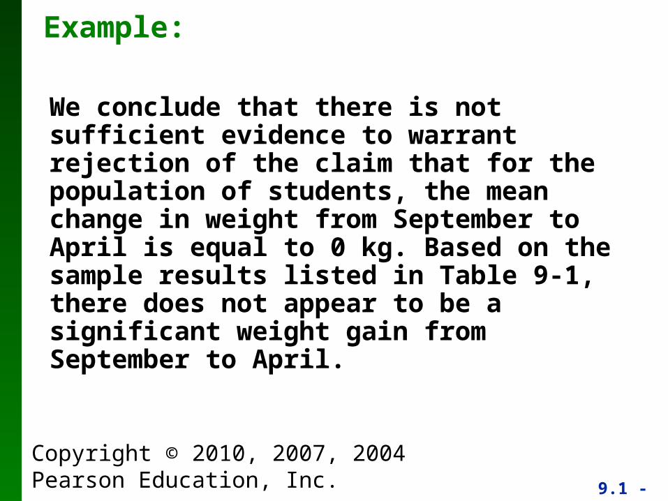
We conclude that there is not sufficient evidence to warrant rejection of the claim that for the population of students, the mean change in weight from September to April is equal to 0 kg. Based on the sample results listed in Table 9-1, there does not appear to be a significant weight gain from September to April.


Example:

The conclusion should be qualified with the limitations noted in the article about the study. The requirement of a simple random sample is not satisfied, because only Rutgers students were used. Also, the study subjects are volunteers, so there is a potential for a self-selection bias. In the article describing the study, the authors cited these limitations and stated that “Researchers should conduct additional studies to better characterize dietary or activity patterns that predict weight gain among young adults who enter college or enter the workforce during this critical period in their lives.”


Example:

The P-value method:Using technology, we can find the P-value of 0.8605. (Using Table A-3 with the test statistic of t = 0.186 and 4 degrees of freedom, we can determine that the P-value is greater than 0.20.) We again fail to reject the null hypothesis, because the P-value is greater than the significance level of = 0.05.


Example:

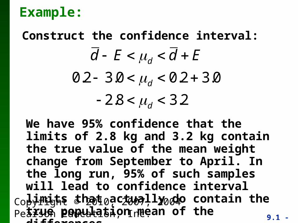
Confidence Interval method:Construct a 95% confidence interval estimate of , which is the mean of the “April–September” weight differences of college students in their freshman year.

= 0.2, sd = 2.4, n = 5, = 2.776

Find the margin of error, E

d

2

2.42.776 3.0

5dsE tn

d

2t


Example:

Construct the confidence interval:

We have 95% confidence that the limits of 2.8 kg and 3.2 kg contain the true value of the mean weight change from September to April. In the long run, 95% of such samples will lead to confidence interval limits that actually do contain the true population mean of the differences.

d E d d E0.2 3.0 d 0.2 3.0

2.8 d 3.2


Recap

In this section we have discussed:

Requirements for inferences from matched pairs.

Notation.

Hypothesis test.

Confidence intervals.

9.1 - 1 copyright © 2010, 2007, 2004 pearson education, inc. section 9-2 inferences about two...

Documents