9 3. u.s. geological survey, eastern geographic science ... · catastrophic wildfire related...
TRANSCRIPT

GDS NWR | Fire Mitigation 1 of 18
Title: 1
Benefits of a Fire Mitigation Ecosystem Service in The Great Dismal Swamp National Wildlife Refuge 2
3
Authors: Bryan Parthum1, Emily Pindilli2, and Dianna Hogan3 4 1. U.S. Geological Survey, Science and Decisions Center, 12201 Sunrise Valley Dr. MSN 913, Reston, 5 Virginia 20192, United States, [email protected] 6 2. U.S. Geological Survey, Science and Decisions Center, 12201 Sunrise Valley Dr. MSN 913, Reston, 7 Virginia 20192, United States, [email protected] 8 3. U.S. Geological Survey, Eastern Geographic Science Center, 12201 Sunrise Valley Drive, MSN 521, 9 Reston, VA 20192, United States, [email protected] 10 11
Abstract 12
The Great Dismal Swamp (GDS) National Wildlife Refuge delivers multiple ecosystem services, 13
including fire mitigation. Our analysis estimates benefits of this service through its potential to reduce 14
catastrophic wildfire related impacts on the health of nearby human populations. We use a combination of 15
high-frequency satellite data, ground sensors, and air quality indices to determine periods of public 16
exposure to dense emissions from a wildfire within the GDS. We examine emergency department (ED) 17
visitation in seven Virginia counties during these periods, apply measures of cumulative Relative Risk 18
(cRR) to derive the effects of wildfire smoke exposure on ED visitation rates, and estimate economic 19
losses using regional Cost of Illness (COI) values established within the US Environmental Protection 20
Agency BenMAP framework. Our results estimate the value of one avoided wildfire within the refuge to 21
be $3.96 million (2015 USD), or $306 per hectare of burn. Reducing the frequency or severity of 22
unexpected and uncontrolled peatland wildfire events has additional benefits not included in this estimate, 23
including costs related to fire suppression during a burn, carbon dioxide emissions, impacts to wildlife, 24
and negative outcomes associated with recreation and regional tourism. We suggest the societal value of 25
the public health benefits alone provides a significant incentive for refuge mangers to implement strategies 26
that will reduce the severity of catastrophic wildfires. 27
28
Keywords 29
Ecosystem services, fire mitigation , wildfire, human health, geospatial information, Great Dismal Swamp 30
National Wildlife Refuge, remote sensing 31
32
33
34
35

GDS NWR | Fire Mitigation 2 of 18
1. Introduction 1
Ecosystem Services (ES) are the benefits provided by the natural environment that are of value to 2
human populations. ES are threatened by development, pollution, fragmentation, overexploitation of 3
resources, and climate change. As part of a multi-year study on the ES of the Great Dismal Swamp (GDS) 4
National Wildlife Refuge, the U.S. Geological Survey (USGS), in coordination with the Fish and Wildlife 5
Service (FWS), examined the economic implications of health effects related to catastrophic peat fire. The 6
GDS is a highly-altered system that has been ditched, drained, and logged, all of which may be increasing 7
the frequency and severity of wildfires (Reddy et al., 2015). The GDS is currently undergoing active 8
hydrologic management designed to rewet the peat soils and provide refuge managers with the ability to 9
actively manage soil moisture using a series of water control structures. These structures are expected to 10
result in multiple benefits including additional carbon sequestration, restoring desired vegetation 11
communities, and reduce the duration and severity of wildfires (Reddy et al., 2015). Sleeter et al. (2017) 12
provides an in depth discussion of the current and desired states within the GDS across multiple 13
dimensions including carbon stock/flow, vegetation, and soil moistures. 14
Benefits of a fire mitigation ecosystem service are closely linked to the health and hydrology of the 15
soils within a peatland ecosystem. Catastrophic wildfire in a peatland is often associated with low water 16
levels, and characterized by long-burning ground fires deep within the peat (>0.5m) that release large 17
quantities of carbon into the atmosphere (Reddy et al., 2015). Within the GDS, low water levels due to 18
centuries of drainage and human disturbance can be worsened in drought years, emphasizing the 19
importance of control and versatility in hydrological management regimes. Conversely, periodic surface 20
wildfires play a critical role in healthy peatland vegetation communities to help perpetuate native trees 21
including Atlantic White Cedar and pond pine (Sleeter et al., 2017; Reddy et al., 2015; Laderman et al., 22
1989). In this paper, we investigate the public health benefits of avoided catastrophic peat wildfires through 23
improved hydrological management, and the implication for adjacent human populations. These benefits 24
are identified as a cost of illness (COI) measure, and are assumed to be a lower bound in the true economic 25
value of reducing wildfire severity and frequency. This assumption is explained in sections 3.2 and 3.3. 26
In recent years, two catastrophic wildfires burned large areas of vegetation within the refuge, 27
producing dense smoke plumes that moved into neighboring communities. The South One Fire of 2008 28
(SOF) was ignited by heavy machinery, burning from June 9th through October 13th, and spanning an 29
estimated 1,976 hectares. During the 121-day burn, the cost of fire suppression exceeded twelve million 30
dollars and distributing smoke into the popular Hampton Roads area of southeastern Virginia, home to an 31
estimated two million people (US Census, 2010). In 2011, the Lateral West Fire, ignited by a lightning 32
strike, swept through the footprint of the SOF burning an estimated 2,630 hectares over the course of 111 33
days from August 4th to December 1st. Both fires quickly destroyed the aboveground vegetation, 34

GDS NWR | Fire Mitigation 3 of 18
concurrently burning deep into the organic peat soils with an average fire depth of 0.8 meters to 1.1 meters 1
(Reddy et al., 2015). Fire events of this magnitude are considered catastrophic and extremely damaging to 2
the ecosystem, and under current conditions are expected to recur twice every 100 years, or an annual 2% 3
probability (MTBS 2014). Emergency department data was made available for high exposure days 4
(explained in section 3.1) during the 2008 SOF, and will be the fire examined within this analysis. 5
Peat soils, such as those within the refuge, have been shown to produce a unique composition of 6
emissions when ignited (Blake, 2009). This combustion results in the intermittent release of dense plumes 7
containing volatile organic compounds, PM2.5 (particulate matter with a diameter of <2.5 µm), and PM10 8
(particulate matter with a diameter of <10 µm), which are considered particularly threatening to the 9
cardiorespiratory health of exposed communities (Geron, 2013; Blake, 2009; Hinwood, 2005; Joseph, 10
2003). 11
The health effects of wildfire emissions have been assessed using a number of different approaches 12
and vary based on geographic location, ignition source, fuel, atmospheric conditions, topography, duration, 13
season, and other physical variations of wildfires (Tse, 2015; Youssouf, 2014; Kochi, 2010 & 2016; 14
Rappold et al., 2011; Vora, 2010). Johnston et al. (2012) emphasize the substantial contribution of 15
landscape fires to harmful global emissions and provide annual mortality estimates resulting from such 16
fires. While in aggregate these estimates are substantial (200k-600k deaths per year globally), Kochi 17
(2016) recommends that mortality should not be considered for individual fire events in the lower quartiles 18
of susceptible acreage, short lived, or infrequent. Wildfires within the GDS are estimated to be both 19
infrequent and on the lower quartiles of susceptible acreage (< 4k hectares) (MTBS, 2014). Following this 20
recommendation we examine effects related to morbidity and assume mortality is not a primary outcome 21
of GDS wildfires. This assumption is supported by the fact that there was no recorded loss of life directly 22
or indirectly attributable to either the 2008 or 2011 GDS wildfires (communication with GDS and FWS 23
staff). Our focus therefore is on symptoms related to morbidity in nearby populations resulting from brief 24
exposure to dense wildfire smoke plumes (EPA, 1999 and 2004). 25
Rappold et al (2011) examined the causal effect of peat fires on emergency department (ED) visitation 26
rates in 42 North Carolina counties during a 2008 catastrophic fire in the Pocosin Lakes National Wildlife 27
Refuge, a peatland with similar vegetation and hydrologic characteristics as those of the GDS. Rappold et 28
al (2011) provide the estimates of cumulative Relative Risk (cRR) used in our analysis. cRR measures the 29
ratio of the probability of a given occurrence over a discreet timeframe; for our purposes, the occurrence 30
ratio is defined as those at risk of an emergency department visit in the absence of harmful smoke exposure, 31
to observed visits during exposure. These calculations are explained in detail in section 3.3. Johnston et 32
al. (2014) employ a similar approach over an eleven-year time period in Sydney, Australia. Using ground-33
based PM sensors they examine the relationship between harmful PM levels due to confirmed fire events 34
GDS NWR | Fire Mitigation 4 of 18
and ED visitation. Although the fuel source of the fires in their study is largely dissimilar to the organic 1
peat soils in our region, they also find a significant relationship (measured in cRR) between ED visitation 2
and smoke exposure days. The likeness of fuel source in Rappold et al (2011) to that of the SOF, and the 3
GDS in general, provides the opportunity for a robust application and extension of their methods. 4
The valuation literature on the economic costs of wildfire is largely focused on geographic areas 5
dissimilar to the GDS (Moeltner, 2013; Richardson, 2012). Richardson et al (2012) employs a defensive 6
behavior method during a 2010 California wildfire to derive willingness to pay (WTP) to avoid smoke 7
exposure. When compared to values derived using COI methods, WTP is considered a more appropriate 8
measure of the true value of fire mitigation services (EPA, 2007; Hanemann, 2001; Loomis, 1991). The 9
authors estimate a WTP/COI ratio of 9:1, suggesting the true value of fire mitigation could potentially be 10
as much as, or more than, nine times higher than COI estimates. Moeltner et al (2013) conducted an 11
intertemporal analysis of wildfires in the western United States and found the marginal effects of wildfires 12
on public health to have a lower-bound of $150-$200 per 40 hectares of wildfire, aggregated to 13
approximately $2.2 million over the course of a fire season in their study area. 14
Our analysis adds to the literature by exploring the economic cost of wildfire through localized 15
outcomes on public health, attributable to wildfire smoke emissions from a nearby forested peat wetland. 16
We extend the wildfire literature by providing unique estimates of the ES benefits resulting from a change 17
in refuge management regimes. Using spatially targeted COI estimates we provide a local measure of the 18
potential benefits to public health as result of improved hydrology and wetland restoration. This study also 19
contributes to a growing body of literature exploring the versatility and applicability of remote sensing 20
methods by using high-frequency satellite data as a foundation for our analysis. Lastly, we propose that 21
the methods described in the following sections may provide a concise and systematic process for 22
researchers and land managers to employ when examining the many benefits of a fire mitigation ecosystem 23
service when larger more in-depth studies are not feasible. Our final estimates rely heavily on the 24
managers’ ability to provide accurate fire probabilities and estimate the reduction in these probabilities as 25
result of their management actions. We recommend the methods in this paper, not the estimates, offer 26
external validity for additional research. The ES benefit estimates are unique to this refuge, and researchers 27
should consider the similarity of their study area to ours before performing any direct transfer of these 28
estimates. 29
30
2. Study Area 31
The GDS encompasses approximately 54,000 hectares of protected habitat located in southeastern Virginia 32
and northeastern North Carolina. Similar to other southern swamps in the eastern United States, the 33
wetland provides a unique habitat for a variety of flora and fauna, and numerous opportunities for 34
GDS NWR | Fire Mitigation 5 of 18
recreational activities. However, the GDS is highly disturbed due to centuries of drainage, logging, and 1
human encroachment, which together have led to drier and less-desirable conditions within the refuge 2
(Reddy et al., 2015). This has shifted fire dynamics within the GDS by exposing organic peat soils to a 3
higher probability of catastrophic wildfire and increasing the frequency and intensity of large fire events 4
(Frost, 1987). In addition to actively managed vegetation through mechanical removal of debris and 5
controlled burns, GDS refuge managers have been developing a grid of culverts and water control 6
structures to aid in the distribution of wetland hydrology with the intent to restore peat moisture to more 7
optimal levels. Our intent is not to provide a full cost/benefit analysis for these management actions, but 8
instead to estimate the benefits of their proposed design. Refuge managers are expected to weigh these 9
benefits with the costs when making their decisions. The refuge sits 40 kilometers inland from the Atlantic 10
coastline, and experiences a west to east atmospheric current. This current typically carries smoke plumes 11
originating from within the GDS out to sea; however, seven Virginia counties (Chesapeake, Isle of Wight, 12
Norfolk City, Portsmouth City, Southampton, Suffolk, and Virginia Beach) surrounding the refuge are 13
prone to smoke exposure from these plumes before they are eventually carried off the coast. Franklin 14
county was omitted due to limitations in acquiring emergency department data. These counties lie within 15
the Tidewater region of Virginia (Appendix I, Figure 1). Five counties in northern North Carolina are 16
suspected to have been exposed to plumes from the SOF as well - Gates, Camden, Currituck, Pasquotank, 17
and Perquimans. However, due to a wildfire in the Pocosin Lakes National Wildlife Refuge during our 18
study period, it is difficult to determine the origin of the smoke over these counties. As such, we limit our 19
study to the seven Tidewater counties to avoid over-estimation of the fire mitigation service. 20
21
3. Materials and Methods 22
Our methodology to estimate the benefits of a fire mitigation ES in GDS was performed in four distinct 23
stages: 1) determine geographic area and populations vulnerable to dense smoke plumes originating within 24
the refuge; 2) apply measures of cRR to health outcomes attributable to wildfire smoke exposure; 3) 25
estimate the economic cost of a wetland wildfire using localized values for COI and lost wages; 4) apply 26
site specific fire probability and forecasted reductions through proposed management actions. The 27
resulting cost estimate is what we consider to be the public health benefit of a fire mitigation ES. 28
29
3.1. Area of impact 30
We determine geographic area and temporal exposure to SOF smoke plumes using a combination of 31
remote sensing techniques, ground-level sensors, and air-quality indices. We examine daily geostationary 32
aerosol smoke product (GASP) satellite readings acquired from the National Environmental Satellite Data 33
and Information Service (NESDIS) for the Tidewater region. These data provide high-resolution measures 34

GDS NWR | Fire Mitigation 6 of 18
of aerosol optical depth (AOD) – at four kilometer square grids - and are collected in 30-minute intervals 1
during daytime hours. AOD is a unitless measure ranging from 0 to 2; higher values indicate dense 2
atmospheric conditions and are considered a good predictor of harmful PM2.5 concentrations (Al-Saadi, 3
2005; EPA, 2009). We generate daily 24-hour averages of AOD measurements for the seven Tidewater 4
counties. 5
In addition to smoke plumes, AOD can also be influenced by ambient air pollution. To help distinguish 6
between pollution and wildfire contributions to AOD measurements, we examine historical levels within 7
the region during both fire and non-fire years. In 2008 during non-fire months (January to June; November 8
and December), the daily AOD average for the Tidewater region was 0.33 with a standard deviation of 9
0.22. Similarly, during non-fire years (2005-‘07; 2009-‘10) AOD averages in the study area were 0.34 10
with a standard deviation of 0.26 (Table 1). The dense nature of the plumes during the SOF can bring these 11
levels up to 2.0. As such, we determine a threshold for harmful smoke exposure to be in excess of 1.25 12
(consistent with assumptions in Rappold et al., 2011), and require at least 10% of the county be exposed 13
above this level. Our estimates rely on these thresholds, we have chosen conservative exposure levels, 14
consistent with the literature, to avoid overestimation in the resulting benefits. Using these parameters, 15
over the 121-day period each of the seven Tidewater counties examined was exposed between one and six 16
days, with a total of 14 days when at least one county received harmful smoke exposure. 17
Satellite-sourced AOD may not always be an appropriate measure of ground level conditions. 18
However, peat wildfires typically result in low-lying smoke plumes, supporting the use of GASP readings 19
when determining human exposure to wildfire smoke plumes (Rappold et al., 2011). An alternative to 20
GASP AOD is to utilize ground level particulate matter measurements from devices within the region. A 21
benefit to ground level monitors is that their 22
elevation is closely representative of human 23
exposure to PM2.5 (Boyouk, 2010); 24
however, there are several limitations 25
associated with these monitors. They have 26
less ability to accurately determine readings 27
across a given region due to their fixed 28
location and the frequency of readings 29
(Youssouf, 2014). For example, some 30
monitors produce values once per day while 31
others are as infrequent as once every four 32
days. Twenty-four hour averages of these 33
readings are a good estimate of high 34
Table 1: Exposure Metrics
Timeframe AOD AQI LRC-PM2.5
Annual
0.34 41.79 10.90
Non-fire
years
(0.26) (18.58) (6.11)
S.O.F. months 0.37 46.98 12.67
(0.24) (20.43) (7.16)
Non-fire
months
0.33 38.09 9.75
(0.22) (17.40) (5.53)
2008 S.O.F. months 0.39 56.76 17.51
(0.24) (34.81) (15.93)
Exposed days
1.45 112.42 46.83
(0.19) (59.92) (32.75) Note: Mean values displayed with standard erros in parentheses. Non-
fire months refers to the months outside of the 121-day S.O.F. burn.
Non-fire years include ‘05-‘07 and ‘09-’10. SOF months of non-fire
years are provided for seasonal reference. Exposed Days are those that
have 24-hour averages ≥ the AOD threshold of 1.25. AQI = Air Quality
Index; LRC=Langly Research Center Monitor; PM2.5 = particulate
matter ≤ 2.5 μg. AOD = aerosol optical depth.

GDS NWR | Fire Mitigation 7 of 18
exposure levels at a given location, but weather patterns may prevent the monitors from detecting high 1
levels of PM2.5 due to wildfire smoke plumes (Youssouf 2014). The NASA Langley Research Center 2
(LRC) is the only ground monitor in the seven-county study area providing daily PM2.5 levels. 7 of the 3
14 exposed days determined using GASP AOD were also days that the ground monitor provided readings. 4
We use these data and the resulting Air Quality Index (AQI) measures of the region to compare estimates 5
of heavy exposure determined by the GASP data (see Table 1). 6
While the 14 GASP AOD high-exposure days also received high PM2.5 estimates from the ground 7
monitor when available, the standard errors are much larger for the LRC ground monitor and AQI. When 8
smoke plumes reach the monitor, this provides a good measure of local air quality; however, much of the 9
Tidewater region isn’t captured by these readings and results in a much larger estimation error for the 10
region. GASP high exposure days have an average AOD of 1.45 and a notably tighter deviation from the 11
mean as they provide a much more spatially and temporally targeted reading derived through the satellite 12
measurements. Over the same months as the SOF in the five non-fire years, the 24-hour AQI average for 13
this region was 46.98. Daily levels of AQI above 63 are considered moderate to unhealthy, and correspond 14
with measured PM2.5 conditions in excess of 35 μg/cm.i The AQI and PM2.5 levels included in Table 1 15
are produced using the U.S. EPA AirData archives.ii 16
17
3.2. Health outcomes 18
We examined the incidence of five cardiorespiratory related 19
illnesses during the SOF. Periods of brief yet heavy exposure to 20
wildfire smoke have been widely recognized to have negative 21
impacts on five specific diagnoses: asthma, chronic obstructive 22
pulmonary disease (COPD), pneumonia/acute bronchitis, 23
congestive heart failure (CHF), and miscellaneous 24
cardiopulmonary symptoms (EPA, 2004 and 1999). These 25
outcomes can by identified by using the International Classification 26
of Diseases, Ninth Division, Clinical Modification (ICD-9-CM) 27
system, which are used by emergency departments to classify patient diagnoses for symptoms of 28
morbidity. Eleven ICD-9-CM codes fall under the five symptoms identified above, and are used in our 29
analysis. In cooperation with Virginia Health Informationiii (VHI) we explore daily ED visits in each of 30
the seven Tidewater counties. Table 2 provides a summary of the symptoms and corresponding ICD-9-31
CM codes. 32
Smoke exposure might not result in an immediate visit to the ED (Pope, 2008; Braga, 2001); as such 33
we consider a window for ED visitation due to a single initial day of heavy smoke exposure. Rappold et 34
Table 2: Disease Classifications
Symptoms ICD-9-CM
Asthma 493
C.O.P.D. 491-492
Pneumonia 481-487
C.H.F. 428
Cardiopulmonary 786 ICD-9-CM = International Classification
of Diseases, Ninth Division, Clinical
Modification system; COPD = chronic
obstructive pulmonary disease; CHF =
congestive heart failure.

GDS NWR | Fire Mitigation 8 of 18
al. (2011) employ a distributed lag model (Peng, 2009) to determine a 5-day lag period in which those 1
who have been exposed to heavy smoke plumes may experience symptoms related to exposure. Following 2
Rappold et al. (2011), we define the visitation window to be the initial day of exposure plus a 5-day lag 3
period. During the SOF there were 548 total ED visits for the eleven ICD-9-CM codes throughout the 4
seven Tidewater counties. 5
Not all the ED visits during the visitation window are a result of the wildfire. A background rate of 6
ED visits for the same symptom classifications would occur regardless of smoke exposure. Rappold et al. 7
(2011) produce estimates of cRR for ED visits associated with brief but heavy exposure to wildfire smoke 8
using a quasi-poisson generalized linear model. Daily estimates of relative risk are then used to determine 9
a measure of cRR over the visitation window. In addition to a point estimate, they establish statistically 10
significant bounds for each symptom. The point estimate and corresponding bounds provide the upper and 11
lower bounds for our valuation estimates. Rappold et al. (2011) explicitly states measures of relative risk 12
to be: 13
𝐷𝑎𝑖𝑙𝑦 𝑅𝑅: 𝑒𝑥𝑝 (𝛽𝑖𝑗𝑡) =𝜇𝑖𝑗𝑡
𝐸𝑥𝑝𝑜𝑠𝑒𝑑
𝜇𝑖𝑗𝑡𝑁𝑜𝑡 𝐸𝑥𝑝𝑜𝑠𝑒𝑑 (1) 14
Equation (1): 𝛽 is determined through the quasi-poisson regression described above; 𝜇 denotes the 15
observed/expected number of visits conditional on exposure; 𝑖, 𝑗, 𝑡 denote the symptom 𝑖 in county 𝑗 on 16
day 𝑡. 17
𝐶𝑢𝑚𝑢𝑙𝑎𝑡𝑖𝑣𝑒 𝑅𝑅: 𝑒𝑥𝑝 (∑ 𝛽𝑖𝑗𝑡) (2)
5
𝑡=0
18
Equation (2): 𝛽𝑖𝑗𝑡 is determined through the distributed lag model (Peng, 2009); 𝑡 denotes the days of 19
visitation from 𝑡 = 0 (day of exposure) to 𝑡 = 5 (lagged exposure days); symptom 𝑖 in county 𝑗. This is 20
the coefficient we use in the following equation to determine excess visits due to the SOF. By applying 21
estimates of cRR for each ICD-9-CM code to the observed visitation during the SOF, we statistically 22
identify the counterfactual - visits not due to the wildfire. Explicitly stated: 23
𝐸𝑥𝑐𝑒𝑠𝑠 𝑉𝑖𝑠𝑖𝑡𝑠 = 𝜇𝑖𝑗𝑡𝐸𝑥𝑝𝑜𝑠𝑒𝑑
− 𝜇𝑖𝑗𝑡
𝐸𝑥𝑝𝑜𝑠𝑒𝑑
exp (∑ 𝛽𝑖𝑗𝑡)5𝑡=0
(3) 24
3.3. Economic Valuation 25
The final step in our analysis is to associate an economic cost with each excess visit from equation 3. 26
We use regional COI values highlighted within the BenMAP model framework (EPA, 2007). BenMAP 27
provides COI by zip code; however, while the estimates vary by diagnosis they remain consistent 28
throughout the Tidewater region. These data and the program are available through www.epa.gov/benmap. 29
While the BenMAP COI estimates incorporate all direct costs of hospitalization associated with each ED 30

GDS NWR | Fire Mitigation 9 of 18
visit by ICD-9-CM diagnoses, they fail to account for the disutility associated with symptoms or lost 1
leisure, and expenses incurred relating to defensive or avoidance behavior. We account for a portion of 2
these costs by using local estimates of symptom days for each hospitalization diagnoses (EPA, 2007) in 3
conjunction with median daily income for each county. We assume individuals to be out of work for the 4
extent of the symptom days. These symptom days do not include time lost during the recovery after the 5
hospital visit, lost productivity, or lost recreation, which have all been shown to significantly increase 6
traditional COI estimates (Chestnut, 2006). To keep our estimates conservative, we only consider lost time 7
during the hospital visit. 8
The likelihood of ED visits and their associated COI are known to vary by age (EPA, 2007), so we 9
consider COI and symptom-day estimates of two age categories. For asthma, COPD, and pneumonia 10
diagnoses, the first age category falls between 18 and 64, and the second is above 64 years of age. For 11
CHF only groups above 65 years of age are considered, and for miscellaneous cardiopulmonary all patients 12
over 18 are a single COI group. These age categories are determined within the BenMAP framework to 13
have different costs and symptom days associated with each diagnoses. We use wages as a proxy to 14
determine the value of time lost during the ED visit. As recommended by the EPA (2007), daily per-capita 15
median income is applied to the number of symptom days associated with each diagnosis. This data is 16
derived from the Bureau of Labor Statisticsiv for each of the seven Tidewater counties. While any group 17
categorized above 64 years of age is assumed to be out of the work force, wages are still used to estimate 18
a portion of the disutility during an ED visit for groups above this age threshold. We aggregate the direct 19
costs of hospitalization (COI) with the opportunity costs (lost wages: LW). Total valuation for the benefits 20
of avoided wildfires in the GDS is calculated using equation (4), an aggregate of values across all seven 21
counties: 22
𝐶𝑜𝑠𝑡 𝑜𝑓 𝑂𝑛𝑒 𝐹𝑖𝑟𝑒 = ∑[𝐸𝑉𝑖𝑗 ∗ (𝐶𝑂𝐼𝑖𝑗
7
𝑗=1
+ 𝐿𝑊𝑖𝑗)] (4) 23
4. Results 24
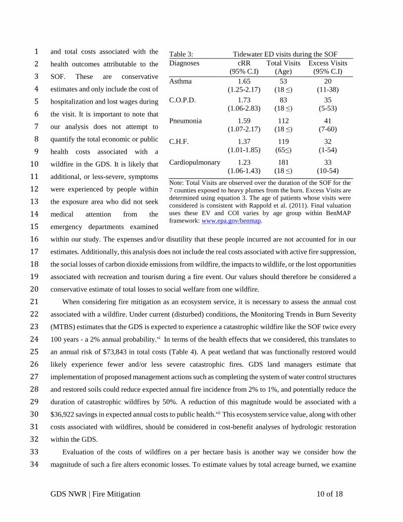
Our analysis indicates that a single catastrophic wildfire event in the GDS results in an estimated 161 25
excess ED visits throughout the seven Tidewater counties. For each symptom, Table 3 provides a summary 26
of measures of cRR, total ED visitation, and ED visitation attributable to the wildfire. The majority of 27
symptoms that resulted in excess ED visits were for morbidity diagnoses surrounding pneumonia, totaling 28
41. An estimated 34 visits were related to COPD, in addition to considerable ED visits for asthma, C.H.F., 29
and other cardiopulmonary symptoms. 30
The economic cost associated with these health effects is an estimated $3.69 million. The upper and 31
lower bounds surrounding our estimate range from $696,475 to $5.73 million, and are a direct result of 32
the 95% confidence interval of the cRR estimates.v Table 4 summarizes the direct COI, opportunity costs, 33
GDS NWR | Fire Mitigation 10 of 18
and total costs associated with the 1
health outcomes attributable to the 2
SOF. These are conservative 3
estimates and only include the cost of 4
hospitalization and lost wages during 5
the visit. It is important to note that 6
our analysis does not attempt to 7
quantify the total economic or public 8
health costs associated with a 9
wildfire in the GDS. It is likely that 10
additional, or less-severe, symptoms 11
were experienced by people within 12
the exposure area who did not seek 13
medical attention from the 14
emergency departments examined 15
within our study. The expenses and/or disutility that these people incurred are not accounted for in our 16
estimates. Additionally, this analysis does not include the real costs associated with active fire suppression, 17
the social losses of carbon dioxide emissions from wildfire, the impacts to wildlife, or the lost opportunities 18
associated with recreation and tourism during a fire event. Our values should therefore be considered a 19
conservative estimate of total losses to social welfare from one wildfire. 20
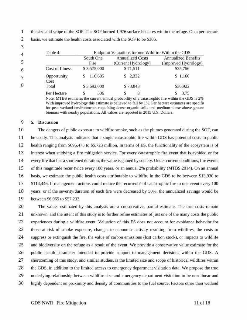
When considering fire mitigation as an ecosystem service, it is necessary to assess the annual cost 21
associated with a wildfire. Under current (disturbed) conditions, the Monitoring Trends in Burn Severity 22
(MTBS) estimates that the GDS is expected to experience a catastrophic wildfire like the SOF twice every 23
100 years - a 2% annual probability.vi In terms of the health effects that we considered, this translates to 24
an annual risk of $73,843 in total costs (Table 4). A peat wetland that was functionally restored would 25
likely experience fewer and/or less severe catastrophic fires. GDS land managers estimate that 26
implementation of proposed management actions such as completing the system of water control structures 27
and restored soils could reduce expected annual fire incidence from 2% to 1%, and potentially reduce the 28
duration of catastrophic wildfires by 50%. A reduction of this magnitude would be associated with a 29
$36,922 savings in expected annual costs to public health.vii This ecosystem service value, along with other 30
costs associated with wildfires, should be considered in cost-benefit analyses of hydrologic restoration 31
within the GDS. 32
Evaluation of the costs of wildfires on a per hectare basis is another way we consider how the 33
magnitude of such a fire alters economic losses. To estimate values by total acreage burned, we examine 34
Table 3: Tidewater ED visits during the SOF
Diagnoses cRR Total Visits Excess Visits
(95% C.I) (Age) (95% C.I)
Asthma 1.65 53 20
(1.25-2.17) (18 ≤) (11-38)
C.O.P.D. 1.73 83 35
(1.06-2.83) (18 ≤) (5-53)
Pneumonia 1.59 112 41
(1.07-2.17) (18 ≤) (7-60)
C.H.F. 1.37 119 32
(1.01-1.85) (65≤) (1-54)
Cardiopulmonary 1.23 181 33
(1.06-1.43) (18 ≤) (10-54)
Note: Total Visits are observed over the duration of the SOF for the
7 counties exposed to heavy plumes from the burn. Excess Visits are
determined using equation 3. The age of patients whose visits were
considered is consistent with Rappold et al. (2011). Final valuation
uses these EV and COI varies by age group within BenMAP
framework: www.epa.gov/benmap.
GDS NWR | Fire Mitigation 11 of 18
the size and scope of the SOF. The SOF burned 1,976 surface hectares within the refuge. On a per hectare 1
basis, we estimate the health costs associated with the SOF to be $306. 2
3
4
5
6
7
8
5. Discussion 9
The dangers of public exposure to wildfire smoke, such as the plumes generated during the SOF, can 10
be costly. This analysis indicates that a single catastrophic fire within GDS has potential costs to public 11
health ranging from $696,475 to $5.723 million. In terms of ES, the functionality of the ecosystem is of 12
interest when studying a fire mitigation service. For every catastrophic fire event that is avoided or for 13
every fire that has a shortened duration, the value is gained by society. Under current conditions, fire events 14
of this magnitude recur twice every 100 years, or an annual 2% probability (MTBS 2014). On an annual 15
basis, we estimate the public health costs attributable to wildfire in the GDS to be between $13,930 to 16
$114,446. If management actions could reduce the recurrence of catastrophic fire to one event every 100 17
years, or if the severity/duration of each fire were decreased by 50%, the annualized savings would be 18
between $6,965 to $57,233. 19
The values estimated by this analysis are a conservative, partial estimate. The true costs remain 20
unknown, and the intent of this study is to further refine estimates of just one of the many costs the public 21
experiences during a wildfire event. Valuation of this ES does not account for avoidance behavior for 22
those at risk of smoke exposure, changes to economic activity resulting from wildfires, the costs to 23
suppress or extinguish the fire, the value of carbon emissions (lost carbon stock), or impacts to wildlife 24
and biodiversity on the refuge as a result of the event. We provide a conservative value estimate for the 25
public health parameter intended to provide support to management decisions within the GDS. A 26
shortcoming of this study, and similar studies, is the limited size and scope of historical wildfires within 27
the GDS, in addition to the limited access to emergency department visitation data. We propose the true 28
underlying relationship between wildfire size and emergency department visitation to be non-linear and 29
highly dependent on proximity and density of communities to the fuel source. Factors other than wetland 30
Table 4: Endpoint Valuations for one Wildfire Within the GDS
South One Annualized Costs Annualized Benefits
Fire (Current Hydrology) (Improved Hydrology)
Cost of Illness $ 3,575,000 $ 71,511 $35,756
Opportunity
Cost
$ 116,605 $ 2,332 $ 1,166
Total $ 3,692,000 $ 73,843 $36,922
Per Hectare $ 306 $ 8 $ 3.75 Note: MTBS estimates the current annual probability of a catastrophic fire within the GDS is 2%.
With improved hydrology this estimate is believed to fall by 1%. Per hectare estimates are specific
for peat wetland environments containing dense organic soils and medium-dense above ground
biomass with nearby populations. All values are reported in 2015 U.S. Dollars.
GDS NWR | Fire Mitigation 12 of 18
hydrology which are likely contribute to this relationship might include public air quality notices and the 1
greater atmospheric patterns which distribute smoke plumes upon various populations. This is an area for 2
future research and we propose this analysis will partner well with studies which examine other factors 3
contributing to the relationship between public health and wildfire or wetland management. 4
Public land managers outside the GDS might find these estimates useful, especially for peat wetland 5
areas susceptible to wildfire, and for management actions aimed at reducing the probability of wildfire for 6
these areas. When doing so, it is important to consider the true underlying costs of wildfires by exploring 7
the use of ratios such as those developed in Richardson (2012), EPA (2007), and Dickie (2004). These 8
ratios are indicative of how high the true value of avoided wildfires could potentially be. Assuming a 9
WTP/COI ratio of 9:1 (Richardson, 2012), our results translate to a WTP in the order of $6.27 million to 10
$51.51 million to avoid a single catastrophic wildfire event. 11
12
6. Conclusions 13
Our analysis adds to the existing literature exploring the economic cost of wildfire through outcomes 14
on public health, attributable to localized wildfire smoke emissions from a nearby forested peat wetland. 15
We extend these costs into management space by providing estimates of the benefits of land management 16
aimed at reducing the duration or severity of wildfire. The methods described above provide a concise and 17
systematic process for researchers and land managers to employ to examine the benefits of a fire mitigation 18
ecosystem service. For this study we were limited to select days of emergency department data during a 19
single historical fire within the GDS. Clearly this is a shortcoming of this study; however, our estimates 20
and methods provide an important contribution to this literature, and we encourage other researchers to 21
replicate these methods in similar wetland areas to help uncover the true underlying relationship between 22
wetland management and public health risks of peat wildfires. Emergency department data such as these 23
are often difficult or costly to acquire. For this reason we propose that a statistically sound functional 24
transfer of the measures of cumulative relative risk from Rappold et al (2011) provides a feasible approach 25
when larger, more in-depth studies are not practical. We also contribute to a growing body of literature 26
exploring the versatility and applicability of remote sensing methods by using high-frequency satellite data 27
as a foundation for our analysis. By using localized COI we propose that the end point estimates derived 28
within our analysis are an accurate value for this region, and any similar research should explore the COI 29
estimates corresponding to the same region as the study. 30
The GDS provides many ecosystem services and the current efforts to restore the wetland’s hydrology 31
could potentially increase the flow of these services. A reduction in the occurrence or severity of 32
catastrophic wildfires in GDS would have multiple benefits including the potential avoidance of negative 33
public health effects. Valuation of the fire mitigation ecosystem service as a part of a portfolio of services 34
GDS NWR | Fire Mitigation 13 of 18
provides important information to refuge management about the total potential benefits associated with 1
wetland restoration. Climate change and continued drying conditions could potentially increase the 2
probability of catastrophic fire, and considering the full range of these valuations will be an important step 3
in protecting the overall welfare of the public. 4

GDS NWR | Fire Mitigation 14 of 18
Appendix I 1
Figure 1: Study Area. Top panel provides total number of days VA counties were exposed
to heavy smoke plumes during the Great Dismal Swamp South One Fire (at least 10% of
county above daily Aerosol Optical Depth (AOD) average of ≥ 1.25). Bottom panel
provides a snapshot of AOD readings for June 21, 2008 when Chesapeake and Virginia
Beach were both above the exposure threshold due to heavy smoke plumes from the SOF.

GDS NWR | Fire Mitigation 15 of 18
Acknowledgements 1
This research is funded and led by the U.S. Geological Survey, Climate and Land Use Change Mission 2
Area as part of LandCarbon. This effort represents one part of a multi-partner project with the U.S. Fish 3
and Wildlife Service, The Nature Conservancy, and George Mason, Clemson, Christopher Newport, East 4
Carolina, and Southern Methodist Universities. The authors acknowledge the collaborative process and 5
those who have contributed their expertise and time (in alphabetical order): Kim Angeli, Karen Balentine, 6
Adam Carver, Nicole Cormier, Colin Daniel, Judith Drexler, Jamie Duberstein, Gary Fisher, Leonardo 7
Frid, Chris Fuller, Joy Greenwood, Laurel Gutenberg, Todd Hawbaker, Ken Krauss, Tim Larson, Courtney 8
Lee, Chris Lowie, Zhong Lu, Rebecca Moss, Christina Musser, Jim Orlando, Chuck Peoples, Howard 9
Phillips, Christine Pickens, Emily Pindilli, John Qu, Brad Reed, Marek Salanski, Josh Salter, John 10
Schmerfeld, Rachel Sleeter, Gary Speiran, Craig Stricker, Brian van Eerden, Sara Ward, Brianna Williams, 11
Fred Wurster, Chris Wright and Zhiliang Zhu. A special acknowledgement to Ana Rappold of the U.S. 12
Environmental Protection Agency for her guidance on transferring measures of cumulative relative risk to 13
the study area. The authors would also like to acknowledge Todd Plessel and James Szykman with the 14
U.S. Environmental Protection Agency for their assistance with and procurement of National 15
Environmental Satellite Data and Information Service (NESDIS) data. A special thank you to Brianna 16
Williams of the USGS who generated the maps in Figure 1. 17
GDS NWR | Fire Mitigation 16 of 18
References 1
Al-Saadi, J., Szykman, J., Pierce, R.B., Kittaka, C., Neil, D., Chu, D.A., Remer, L., Gumley, L., Prins, E., Weinstock, 2 L., Macdonald, C., Wayland, R., Dimmick, F., Fishman, J., 2005.Improving National Air Quality Forecasts with 3 Satellite Aerosol Observations. Bulletin of the American Meteorological Society 86, 1249–1261. doi:10.1175/bams-4 86-9-1249 5
Blake, D., Hinwood, A., Horwitz, P., 2009. Peat fires and air quality: Volatile organic compounds and particulates. 6 Chemosphere. 76:419–423. doi:10.1016/j.chemosphere.2009.03.047 7
Boyouk, N., Léon, J.-F., Delbarre, H., Podvin, T., Deroo, C., 2010. Impact of the mixing boundary layer on the 8 relationship between PM2.5 and aerosol optical thickness. Atmospheric Environment 44, 271–277. 9 doi:10.1016/j.atmosenv.2009.06.053 10
Braga, A.C., Zanobetti, A., Schwartz, J., 2001. The Lag Structure Between Particulate Air Pollution and Respiratory 11 and Cardiovascular Deaths in 10 US Cities. Journal of Occupational and Environmental Medicine 43, 927–933. 12 doi:10.1097/00043764-200111000-00001 13
[dataset] Bureau of Labor Statistics: https://www.bls.gov/data/#wages 14
Chestnut, L.G., Thayer, M.A., Lazo, J.K., Eeden, S.K., 2006. The Economic Value Of Preventing Respiratory And 15 Cardiovascular Hospitalizations. Contemporary Economic Policy 24, 127–143. doi:10.1093/cep/byj007 16
Dickie, M., Messman, V.L., 2004. Parental altruism and the value of avoiding acute illness: are kids worth more than 17 parents? Journal of Environmental Economics and Management 48, 1146–1174. doi:10.1016/j.jeem.2003.12.005 18
Frost, C.C. 1987. Historical overview of Atlantic White-cedar in the Carolinas. A.D. Laderman, Atlantic White-cedar 19 Wetlands, Westview Press. 257–263. 20
Geron, C., Hays, M., 2013. Air emissions from organic soil burning on the coastal plain of North Carolina. 21 Atmospheric Environment 64, 192–199. doi:10.1016/j.atmosenv.2012.09.065 22
Hanemann, M., Kanninen, B., 2001. The Statistical Analysis of Discrete‐Response CV Data. Valuing Environmental 23 Preferences 302–441. doi:10.1093/0199248915.003.0011 24
Hinwood, A.L., and C.M. Rodriguez. 2005. Potential Health Impacts Associated with Peat Smoke: A Review. Journal 25 of the Royal Society of Western Australia, 88:133-138. 26
Johnston F., Henderson S., Chen Y., Randerson J., Marlier M, DeFries R., Kinney P., Bowman D., Brauer M. 2012. 27 Estimated global mortality attributable to smoke from landscape fires. Environ. Health Perspect. 120 (5): 659-701. 28 doi:10.1289/ehp.1104422 29
Johnston, F., Purdie, S., Jalaludin, B., Martin, K., Henderson, S., Morgan, G. 2014. Air pollution events from forest 30 fires and emergency department attendances in Sydney, Australia 1996-2007: a case-crossover analysis. 31 Environmental Health 2014 13:105. doi:10.1186/1476-069X-13-105 32
Joseph, A., Sawant, A., Srivastava, A., 2003. PM10 and its impacts on health - a case study in Mumbai. International 33 Journal of Environmental Health Research 13, 207–214. doi:10.1080/0960312031000098107 34
Kochi, I., Champ, P.A., Loomis, J.B., Donovan, G.H., 2016. Valuing morbidity effects of wildfire smoke exposure 35 from the 2007 Southern California wildfires. Journal of Forest Economics 25, 29–54. doi:10.1016/j.jfe.2016.07.002 36
Kochi, I., Donovan, G.H., Champ, P.A., Loomis, J.B., 2010. The economic cost of adverse health effectsfrom 37 wildfire-smoke exposure: a review. International Journal of Wildland Fire 19, 803. doi:10.1071/wf09077 38
GDS NWR | Fire Mitigation 17 of 18
Laderman, Aimlee D. and Brody, Michael and Pendleton , Edward 1989. The ecology of Atlantic white cedar 1 wetlands: a community profile. Washington, D.C., U.S. Department of Interior, Fish and Wildlife Service, National 2 Wetlands Research Center, 114pp. Biological Report.857.21. http://www.nwrc.usgs.gov/techrpt/85-7-21.pdf 3
Loomis, J., Hanemann, M., Kanninen, B., Wegge, T., 1991. Willingness to Pay to Protect Wetlands and Reduce 4 Wildlife Contamination from Agricultural Drainage. The Economics and Management of Water and Drainage in 5 Agriculture 411–429. doi:10.1007/978-1-4615-4028-1_21 6
Moeltner, K., Kim, M.-K., Zhu, E., Yang, W., 2013. Wildfire smoke and health impacts: A closer look at fire 7 attributes and their marginal effects. Journal of Environmental Economics and Management 66, 476–496. 8 doi:10.1016/j.jeem.2013.09.004 9
[dataset] Monitoring Trends in Burn Severity MTBS. Data Access: Fire Level Geospatial Data. US Department of 10 Agriculture, Forest Service and US Department of Interior, Geological Survey. 2014. 11 http://mtbs.gov/data/individualfiredata.html/. Accessed 10 Sept 2015. 12
Peng, R., Dominici, F., Welty, L.J., 2009. A Bayesian hierarchical distributed lag model for estimating the time 13 course of risk of hospitalization associated with particulate matter air pollution. Journal of the Royal Statistical 14 Society: Series C (Applied Statistics) 58, 3–24. doi:10.1111/j.1467-9876.2008.00640.x 15
Pope, C., Renlund, D., Kfoury, A., May, H., Horne, B., 2008. Relation of Heart Failure Hospitalization to Exposure 16 to Fine Particulate Air Pollution. The American Journal of Cardiology 102, 1230–1234. 17 doi:10.1016/j.amjcard.2008.06.044 18
Rappold, A., Stone, S., Cascio, W., Neas, L., Kilaru, V., Carraway, M., Szykman, J., Ising, A., Cleve, W.E., Meredith, 19 J.T., Vaughan-Batten, H., Deyneka, L., Devlin, R.B., 2011. Peat Bog Wildfire Smoke Exposure in Rural North 20 Carolina Is Associated with Cardiopulmonary Emergency Department Visits Assessed through Syndromic 21 Surveillance. Environmental Health Perspectives 119, 1415–1420. doi:10.1289/ehp.1003206 22
Reddy, A., Hawbaker, T., Wurster, F., Zhu, Z., Ward, S., Newcomb, D., Murray, R., 2015. Quantifying soil carbon 23 loss and uncertainty from a peatland wildfire using multi-temporal LiDAR. Remote Sensing of Environment 170, 24 306–316. doi:10.1016/j.rse.2015.09.017 25
Richardson, L.A., Champ, P.A., Loomis, J.B., 2012. The hidden cost of wildfires: Economic valuation of health 26 effects of wildfire smoke exposure in Southern California. Journal of Forest Economics 18, 14–35. 27 doi:10.1016/j.jfe.2011.05.002 28
Sleeter, R., Sleeter, B., Williams, B., Hogan, D., Hawbakaer, T., Zhiliang, Z., 2017. A carbon balance model for the 29 great dismal swamp ecosystem. Carbon Balance Manage (2017) 12:2. doi:10.1186/s13021-017-0070-4 30
Tse, K., Chen, L., Tse, M., Zuraw, B., Christiansen, S., 2015. Effect of catastrophic wildfires on asthmatic outcomes 31 in obese children: breathing fire. Annals of Allergy, Asthma & Immunology 114. doi:10.1016/j.anai.2015.01.018 32
U.S. Census Bureau, Population Division. 2010. https://census.gov/ 33
[dataset] U.S. Environmental Protection Agency EPA AirData archives: https://www.epa.gov/outdoor-air-quality-34 data/download-daily-data 35
U.S. Environmental Protection Agency EPA. 1999. The Benefits and Costs of the Clean Air Act 1990 to 2010. US 36 Environmental Protection Agency: Washington, DC. 37
U.S. Environmental Protection Agency EPA. 2004. Air Quality Criteria for Particulate Matter. US Environmental 38 Protection Agency: Washington, DC. 39
GDS NWR | Fire Mitigation 18 of 18
U.S. Environmental Protection Agency EPA. 2007. Cost of Illness Handbook. US Environmental Protection Agency: 1 Washington DC. 2
U.S. Environmental Protection Agency EPA. 2009. Air Quality Index, A Guide to Air Quality and Your Health. 3 EPA-456/F-409-002. Research Triangle Park, NC:U.S. EPA. 4
Vora, C., Renvall, M., Chao, P., Ferguson, P., Ramsdell, J., 2010. How the October 2007 San Diego Wildfires 5 Affected Asthmatics. Journal of Allergy and Clinical Immunology 125. doi:10.1016/j.jaci.2009.12.811 6
Youssouf, H., Liousse, C., Roblou, L., Assamoi, E., Salonen, R., Maesano, C., Banerjee, S., Annesi-Maesano, I., 7 2014. Quantifying wildfires exposure for investigating health-related effects. Atmospheric Environment 97, 239–8 251. doi:10.1016/j.atmosenv.2014.07.041 9
i Additional information regarding the AQI can be accessed through the U.S. EPA and/or AirNow.gov ii EPA AirData archives: https://www.epa.gov/outdoor-air-quality-data/download-daily-data iii ED visits during the duration of the SOF burn were made available to the researchers through Virginia Health
Information for the current analysis and under privacy agreements cannot be released. iv Bureau of Labor Statistics provides wage data by county: https://www.bls.gov/data/#wages v These confidence intervals are listed in Table 3 under the point estimate for each estimate of cRR. To create the
upper and lower bounds in our valuation, these values were used in equation 3. vi Monitoring Trends in Burn Severity (MTBS) provides 30 years of historical data to determine fire probabilities for
the GDS. Recent scenarios suggest annual probabilities could in fact be larger, especially when coupled with climate
change projections. vii Peat wetland hydrologic restoration and water control structures are expected to contribute to the reduced
magnitude of impacts (especially duration) of wildfires and potentially reduced incidence; however, the precise
effects are not fully understood. Therefore, we use 50% reductions in duration and/or incidence as a hypothetical to
illustrate the potential value of avoided health effects.