8.2 Stability and classification of isolated critical points

Stability and classification of isolated critical points

Isolated critical points

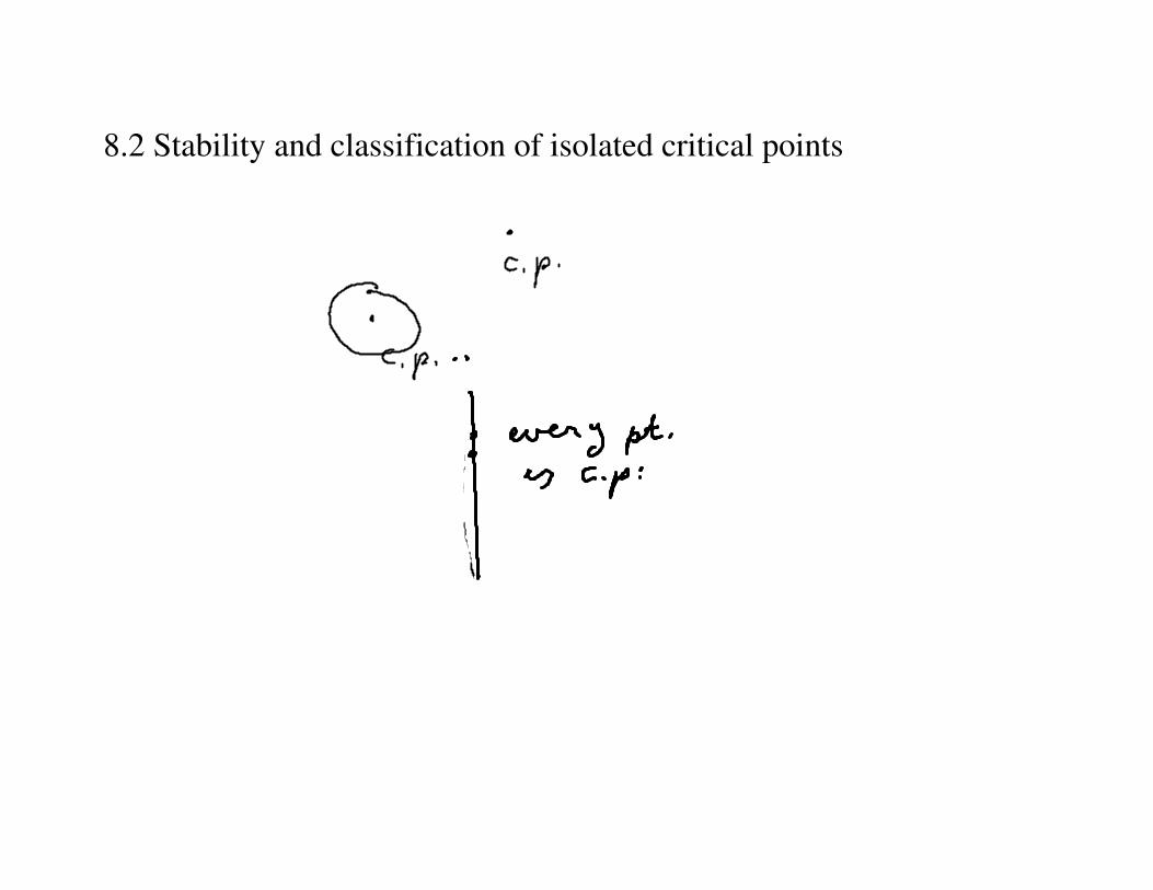
A critical point is isolated if it is the only critical point in somesmall neighborhood of the point.

If we zoom in far enough on an isolated critical point, it is the onlycritical point we see.

In the system x � = y , y � = −x + x2 or [ xy ]� =

� y−x+x2

�,

the critical point (x0, y0) = (1, 0) is isolated because it is theonly critical point in any circle of small radius centered at (1, 0).

Example with non-isolated critical points

For the system x � = x , y � = x2, any point (x , y) with x = 0 is acritical point: the entire y−axis consists of critical points.

Consider the critical point (x0, y0) = (0, 1).No matter how far we zoom in on this point,there will always be other points on the y−axis visible:the critical point (0, 1) is not isolated.

For the SIR model of epidemiology, with x = fraction infected,y = fraction recovered and (1− x − y) = fraction susceptible,

x � = (2.5(1− x − y)− 1)x

y � = x

any point (x , y) with x = 0 is a critical point.The entire y−axis consists of critical points that are not isolated.

Classification of isolated critical points

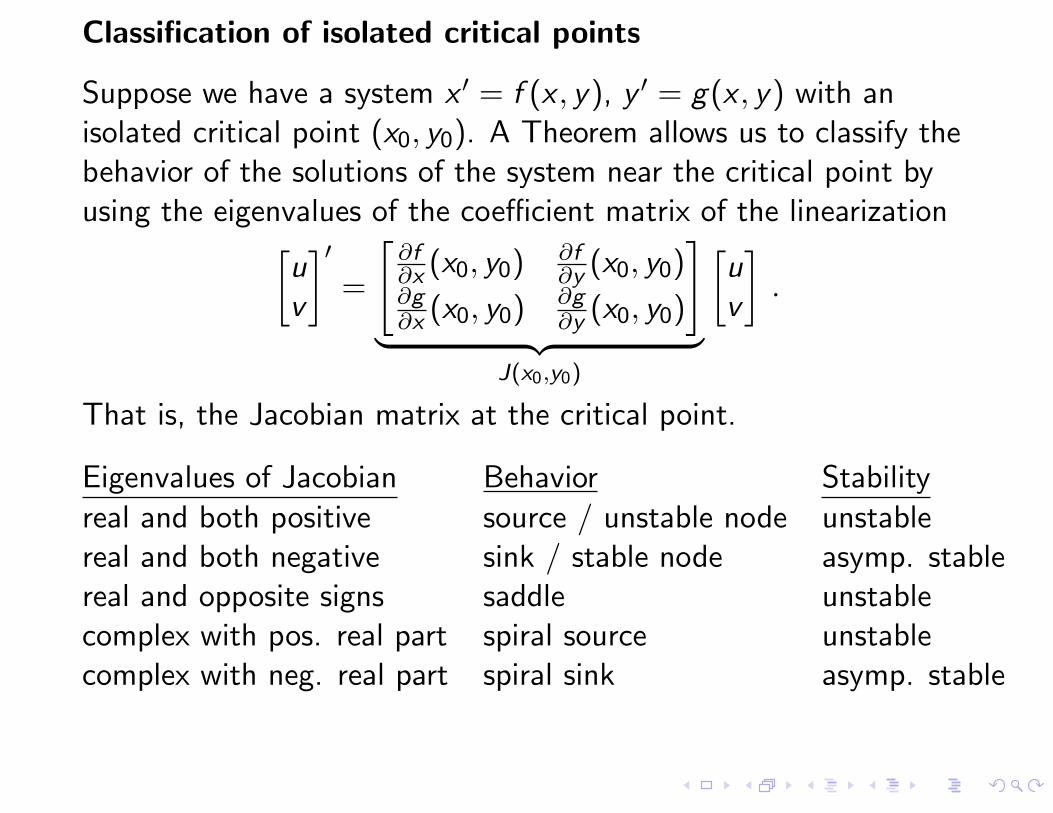
Suppose we have a system x � = f (x , y), y � = g(x , y) with anisolated critical point (x0, y0). A Theorem allows us to classify thebehavior of the solutions of the system near the critical point byusing the eigenvalues of the coefficient matrix of the linearization

�uv

��=

�∂f∂x (x0, y0)

∂f∂y (x0, y0)

∂g∂x (x0, y0)

∂g∂y (x0, y0)

�

� �� �J(x0,y0)

�uv

�.

That is, the Jacobian matrix at the critical point.

Eigenvalues of Jacobian Behavior Stability

real and both positive source / unstable node unstablereal and both negative sink / stable node asymp. stablereal and opposite signs saddle unstablecomplex with pos. real part spiral source unstablecomplex with neg. real part spiral sink asymp. stable

Stable, unstable and asymptotically stable critical points

A stable critical point (x0, y0) is one where given any smalldistance � to (x0, y0), and any initial condition within a perhapssmaller radius around (x0, y0), the trajectory of the system nevergoes further away from (x0, y0) than �.

A stable critical point (x0, y0) is called asymptotically stable ifgiven any initial condition sufficiently close to (x0, y0) and anysolution

�x(t), y(t)

�satisfying that condition, then

limt→∞

�x(t), y(t)

�= (x0, y0).

An unstable critical point is one that is not stable.

Example: Stability of critical points for [ xy ]� =

�−y−x2

−x+y2

�

Critical points are where −y − x2 = 0 and −x + y2 = 0.The first equation means y = −x2, and plugging into the secondequation we obtain −x + x4 = 0.Factoring we obtain x(1− x3) = 0. Since we are looking only forreal solutions we get either x = 0 or x = 1.Solving for the corresponding y using y = −x2, we get two criticalpoints, (0, 0) and (1,−1), isolated since a positive distance apart.

Let us compute the Jacobian matrix: J(x , y) =�−2x −1

−1 2y

�.

At the point (0, 0) we get the matrix J(0, 0) =�

0 −1−1 0

�.

The two eigenvalues are 1 and −1, real and of opposite signs.From the table, we get a saddle, which is an unstable critical point.

Example: Stability of critical points for [ xy ]� =

�−y−x2

−x+y2

�(ctd)

Recall the Jacobian matrix J(x , y) =�−2x −1

−1 2y

�.

At the point (1,−1) we get J(1,−1) =�−2 −1−1 −2

�.

The two eigenvalues are −1, −3, real and both negative, so thecritical point is a sink, and therefore an asymptotically stableequilibrium point.

if we start with any initial point (x(0), y(0)) close to (1,−1) andplot a trajectory, it approaches (1,−1).In other words,

limt→∞

�x(t), y(t)

�= (1,−1).

Centers in linear systems

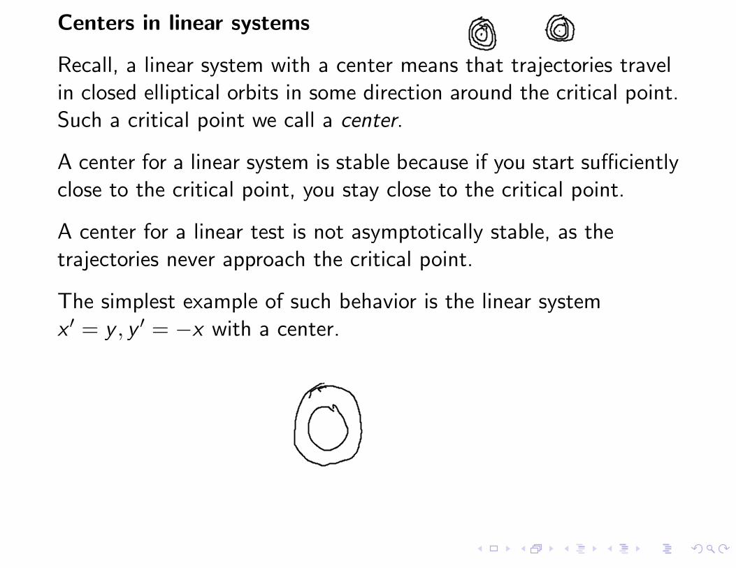
Recall, a linear system with a center means that trajectories travelin closed elliptical orbits in some direction around the critical point.Such a critical point we call a center.

A center for a linear system is stable because if you start sufficientlyclose to the critical point, you stay close to the critical point.

A center for a linear test is not asymptotically stable, as thetrajectories never approach the critical point.

The simplest example of such behavior is the linear systemx � = y , y � = −x with a center.

Nonlinear systems whose linearizations have centers

An example is x � = y , y � = −x + y3.The only critical point is the origin (0, 0), where the Jacobianmatrix is

�0 1−1 0

�, with eigenvalues ±i .

The linearization has a center.

Take a trajectory starting at (x(0), y(0)) near the origin.The trajectory then goes around the origin, butddt (x

2 + y2) = 2xx � + 2yy � = 2xy − 2xy + 2y4 = 2y4 ≥ 0, so thedistance from (x(t), y(t)) to the origin increases with t and thetrajectory is an outward spiral. With more detail, this argumentcan be used to show the origin is unstable.

Another example is x � = y , y � = −x − y3. Note the sign of the y3

term. The trajectories for this new system are inward spirals, andthe origin is asymptotically stable.

Nonlinear systems whose linearizations have centers (ctd 1)

The three systems1) x � = y , y � = −x2) x � = y , y � = −x + y3

3) x � = y , y � = −x − y3

all have the same critical point (0, 0) andall have the same linearization x � = y , y � = −x .

However,for 1), the critical point is a center,for 2), the critical point is a spiral source, andfor 3), the critical point is a spiral sink.

This demonstrates the “trouble with centers”:if the linearization has a center, additional analysis of thenonlinearity in the original system is still needed to classify thecritical point.

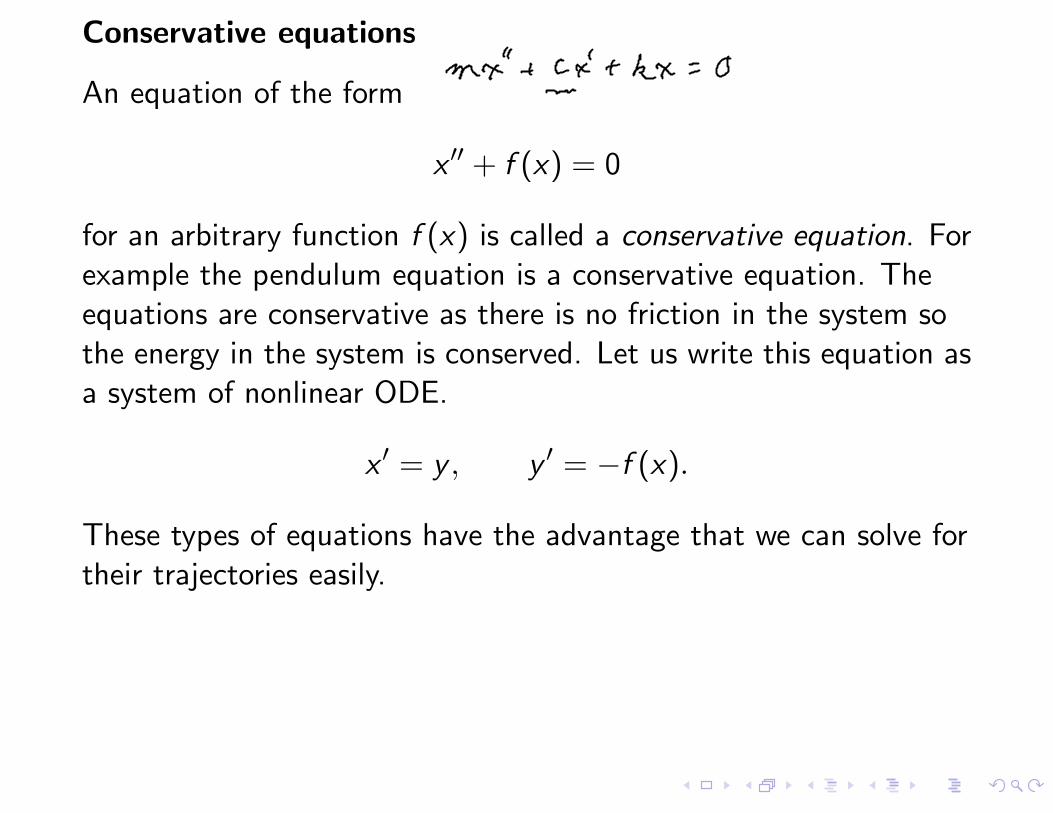
Conservative equations

An equation of the form

x �� + f (x) = 0

for an arbitrary function f (x) is called a conservative equation. Forexample the pendulum equation is a conservative equation. Theequations are conservative as there is no friction in the system sothe energy in the system is conserved. Let us write this equation asa system of nonlinear ODE.

x � = y , y � = −f (x).

These types of equations have the advantage that we can solve fortheir trajectories easily.

Conservative equations (ctd 1)

Think of y as a function of x thenhen use the chain rule

x �� = y � =dy

dxx � = y

dy

dx,

where the prime indicates a derivative with respect to t. We obtainy dydx + f (x) = 0. We integrate with respect to x to get�y dydx dx +

�f (x) dx = C . In other words

1

2y2 +

�f (x) dx = C ,

an implicit equation for the trajectories, with different C givingdifferent trajectories. This expression is sometimes called theHamiltonian or the energy of the system. If you look back tonotice that y dy

dx + f (x) = 0 is an exact equation, and we just founda potential function.

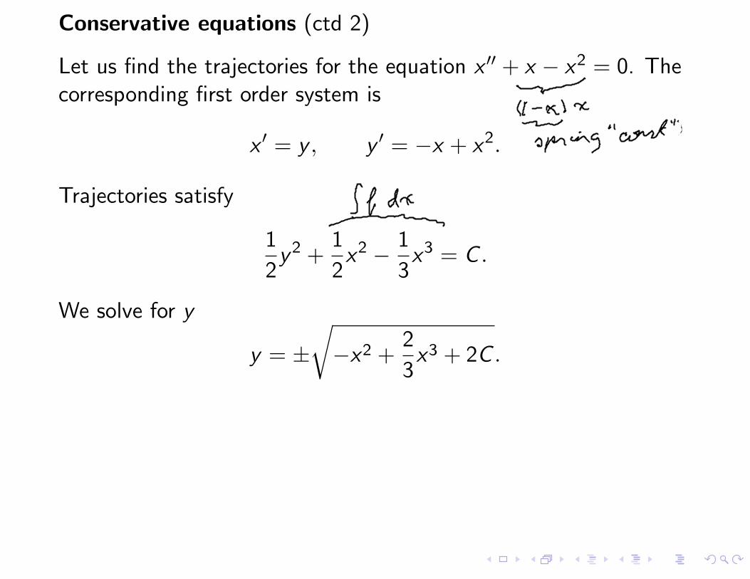
Conservative equations (ctd 2)

Let us find the trajectories for the equation x �� + x − x2 = 0. Thecorresponding first order system is

x � = y , y � = −x + x2.

Trajectories satisfy

1

2y2 +

1

2x2 − 1

3x3 = C .

We solve for y

y = ±�

−x2 +2

3x3 + 2C .

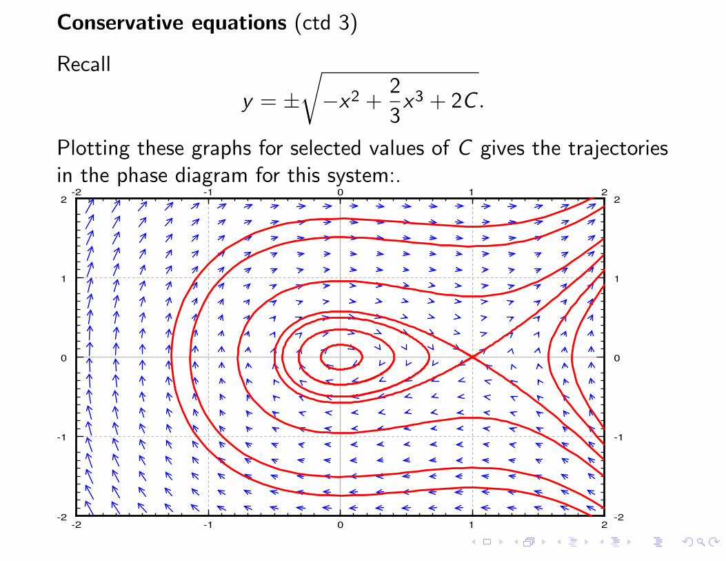
Conservative equations (ctd 3)

Recall

y = ±�

−x2 +2

3x3 + 2C .

Plotting these graphs for selected values of C gives the trajectoriesin the phase diagram for this system:.

-2 -1 0 1 2

-2 -1 0 1 2

-2

-1

0

1

2

-2

-1

0

1

2

Conservative equations (ctd 4)

We notice that near the origin the trajectories are closed curves:they keep going around the origin, never spiraling in or out.Therefore we discovered a way to verify that the critical point at(0, 0) is a stable center.

The critical point at (0, 1) is a saddle as we already noticed.

8.3 Applications of nonlinear systems

Applications of nonlinear systems

Pendulum

The pendulum equation is θ�� + gL sin θ = 0. Here, θ is the angular

displacement, g is the gravitational acceleration, and L the lengthof the pendulum. There is no friction: the equation is conservative.

Let us change the equation to a two-dimensional system invariables (θ,ω) by introducing ω = θ�:

�θω

��=

�ω

−gL sin θ

�.

Pendulum (ctd 1)

The critical points of this system are when ω = 0 and sin θ = 0.These points are . . . (−2π, 0), (−π, 0), (0, 0), (π, 0), (2π, 0) . . ..

There are infinitely many critical points, all isolated.For conservative equations, there are two types of critical points:saddle points and centers.

Let us compute the Jacobian matrix:

∂∂θ

�ω�

∂∂ω

�ω�

∂∂θ

�−g

L sin θ�

∂∂ω

�−g

L sin θ� =

�0 1

−gL cos θ 0

�.

The eigenvalues of the Jacobian matrix are λ = ±�

−gL cos θ.

The eigenvalues are going to be purely imaginary when cos θ > 0.This happens at the even multiples of π.

The eigenvalues are real when cos θ < 0.This happens at the odd multiples of π.

Pendulum (ctd 2)

Therefore the system has a stable center at the points. . . (−2π, 0), (0, 0), (2π, 0) . . ., and it has an unstable saddle at thepoints . . . (−3π, 0), (−π, 0), (π, 0), (3π, 0) . . .. Look at the phasediagram in where for simplicity we let g

L = 1.

-5.0 -2.5 0.0 2.5 5.0

-5.0 -2.5 0.0 2.5 5.0

-3

-2

-1

0

1

2

3

-3

-2

-1

0

1

2

3

The horizontal axis is the deflection angle. The vertical axis is theangular velocity of the pendulum.

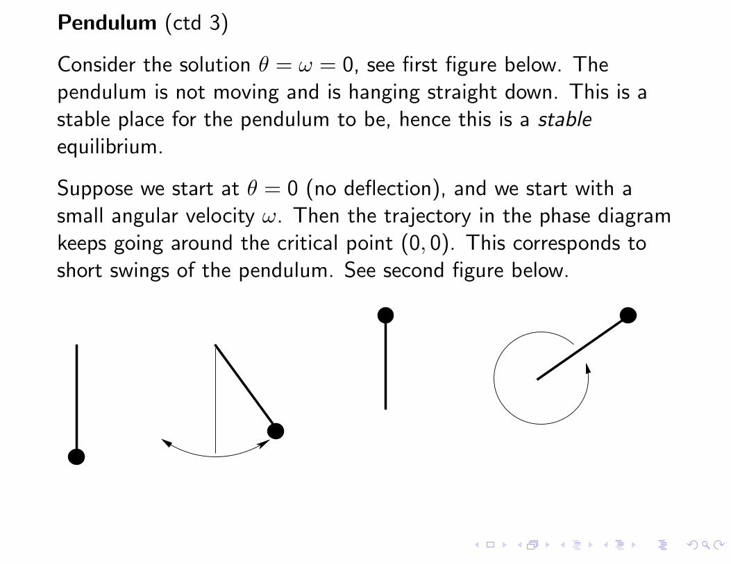
Pendulum (ctd 3)

Consider the solution θ = ω = 0, see first figure below. Thependulum is not moving and is hanging straight down. This is astable place for the pendulum to be, hence this is a stableequilibrium.

Suppose we start at θ = 0 (no deflection), and we start with asmall angular velocity ω. Then the trajectory in the phase diagramkeeps going around the critical point (0, 0). This corresponds toshort swings of the pendulum. See second figure below.

Pendulum (ctd 4)

Consider the solution θ = π, ω = 0. The pendulum is upside down.Although you can balance the pendulum this way, this is anunstable equilibrium. Even the tiniest push will make thependulum start swinging wildly. See third figure above.

Suppose we start at θ = 0 but give the pendulum a big enoughpush, ω = θ�(0) > 0, It goes over the top and keeps spinning. Thisbehavior corresponds to the top wavy curves in the phase diagramthat do not cross the horizontal axis. See fourth figure above.

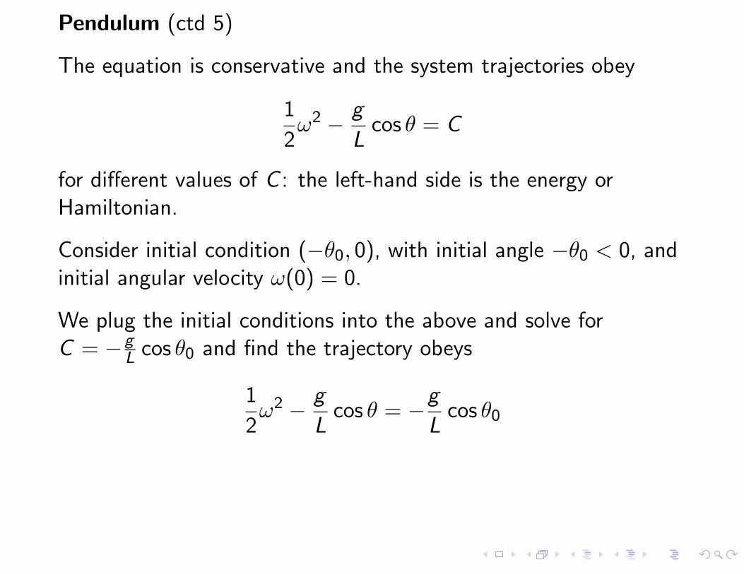
Pendulum (ctd 5)

The equation is conservative and the system trajectories obey

1

2ω2 − g

Lcos θ = C

for different values of C : the left-hand side is the energy orHamiltonian.

Consider initial condition (−θ0, 0), with initial angle −θ0 < 0, andinitial angular velocity ω(0) = 0.

We plug the initial conditions into the above and solve forC = −g

L cos θ0 and find the trajectory obeys

1

2ω2 − g

Lcos θ = −g

Lcos θ0

Pendulum (ctd 6)

Consider the first half pendulum swing, from angle −θ0 to θ0.During this motion, ω = θ� ≥ 0 so we must choose the plus sign:

ω = +

�2g

L

�cos θ − cos θ0.

Since ω = dθdt , inverting we get

dt

dθ=

�L

2g

1√cos θ − cos θ0

.

The time T1/2 the pendulum takes to swing from −θ0 to θ0 is then

T 12=

�L

2g

� θ0

−θ0

1√cos θ − cos θ0

dθ

Pendulum (ctd 7)

The period T is then

T = 2T 12= 4

�L

2g

� θ0

0

1√cos θ − cos θ0

dθ

The integral is an improper integral, and we cannot in generalevaluate it symbolically. We must resort to numericalapproximation if we want to compute a particular T . Recall� + g

Lθ = 0 has period

Tlinear = 2π

�L

g.

Note that Tlinear is simply a constant, it does not change with theinitial angle θ0. The actual period T gets larger and larger as θ0gets larger.

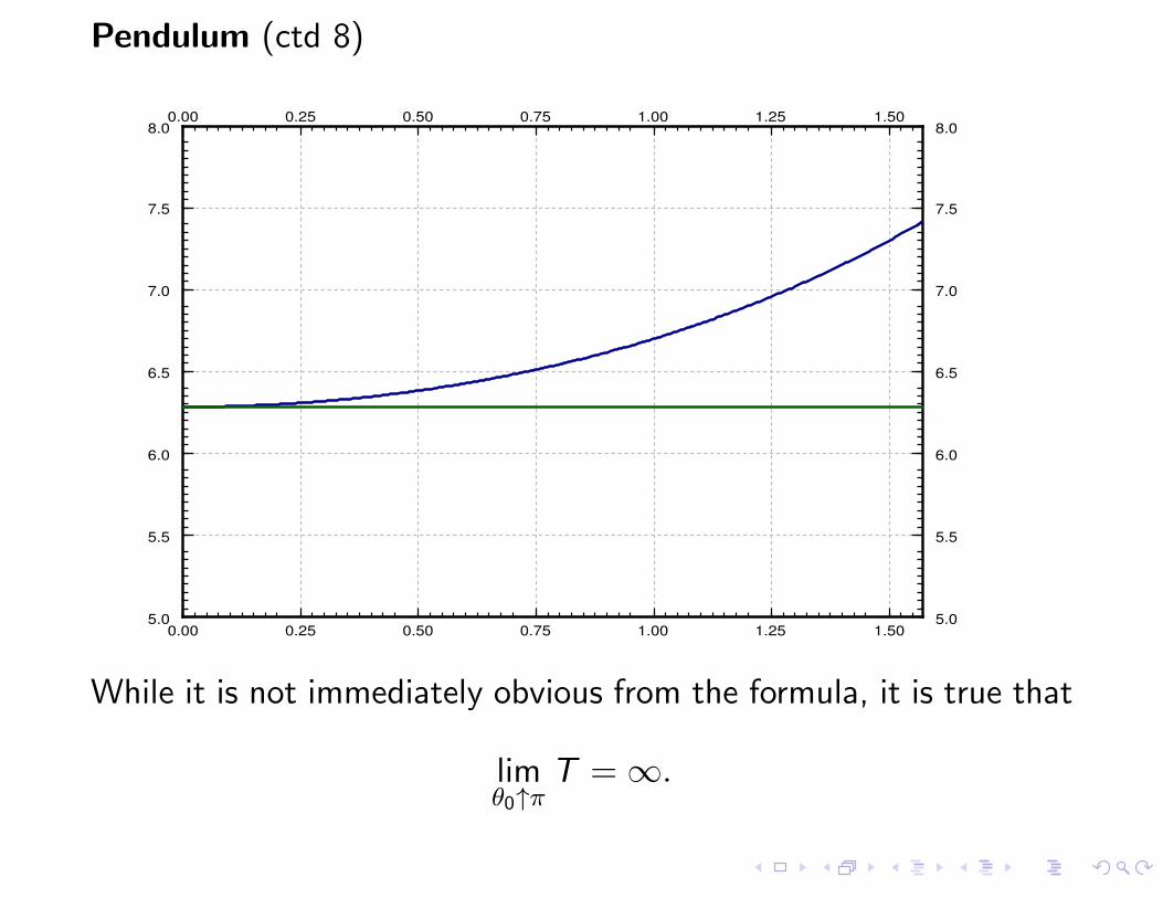
Pendulum (ctd 8)

0.00 0.25 0.50 0.75 1.00 1.25 1.50

0.00 0.25 0.50 0.75 1.00 1.25 1.50

5.0

5.5

6.0

6.5

7.0

7.5

8.0

5.0

5.5

6.0

6.5

7.0

7.5

8.0

While it is not immediately obvious from the formula, it is true that

limθ0↑π

T = ∞.

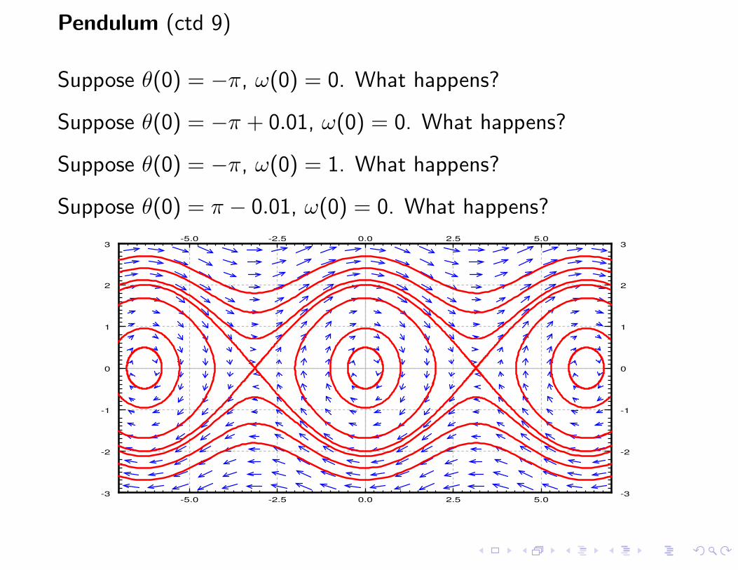
Pendulum (ctd 9)

Suppose θ(0) = −π, ω(0) = 0. What happens?

Suppose θ(0) = −π + 0.01, ω(0) = 0. What happens?

Suppose θ(0) = −π, ω(0) = 1. What happens?

Suppose θ(0) = π − 0.01, ω(0) = 0. What happens?

-5.0 -2.5 0.0 2.5 5.0

-5.0 -2.5 0.0 2.5 5.0

-3

-2

-1

0

1

2

3

-3

-2

-1

0

1

2

3