804 ieee transactions on control systems …tomlin/papers/journals/brt06_tcst.pdf · 804 ieee...

804 IEEE TRANSACTIONS ON CONTROL SYSTEMS TECHNOLOGY, VOL. 14, NO. 5, SEPTEMBER 2006

Adjoint-Based Control of a New Eulerian NetworkModel of Air Traffic Flow

Alexandre M. Bayen, Member, IEEE, Robin L. Raffard, and Claire J. Tomlin, Member, IEEE

Abstract—An Eulerian network model for air traffic flow in theNational Airspace System is developed and used to design flowcontrol schemes which could be used by Air Traffic Controllersto optimize traffic flow. The model relies on a modified version ofthe Lighthill–Whitham–Richards (LWR) partial differential equa-tion (PDE), which contains a velocity control term inside the diver-gence operator. This PDE can be related to aircraft count, whichis a key metric in air traffic control. An analytical solution to theLWR PDE is constructed for a benchmark problem, to assess thegridsize required to compute a numerical solution at a prescribedaccuracy. The Jameson–Schmidt–Turkel (JST) scheme is selectedamong other numerical schemes to perform simulations, and evi-dence of numerical convergence is assessed against this analyticalsolution. Linear numerical schemes are discarded because of theirpoor performance. The model is validated against actual air trafficdata (ETMS data), by showing that the Eulerian description en-ables good aircraft count predictions, provided a good choice ofnumerical parameters is made. This model is then embedded asthe key constraint in an optimization problem, that of maximizingthe throughput at a destination airport while maintaining aircraftdensity below a legal threshold in a set of sectors of the airspace.The optimization problem is solved by constructing the adjointproblem of the linearized network control problem, which providesan explicit formula for the gradient. Constraints are enforced usinga logarithmic barrier. Simulations of actual air traffic data andcontrol scenarios involving several airports between Chicago andthe U.S. East Coast demonstrate the feasibility of the method.

Index Terms—Adjoint-based optimization, control of partial dif-ferential equations, LWR PDE.

I. INTRODUCTION

THE National Airspace System (NAS) consists of aircraft,control facilities, procedures, navigation and surveillance

equipment, analysis equipment, decision support tools, and con-troller pilots who operate the systems. In this article, the focus istraffic flow management (TFM), which has the goal to maximizethroughput while maintaining safety. This entails the design ofefficient methods to route aircraft, while preventing the densityof aircraft from becoming too large in regions of airspace, and op-erating efficient reroutes when the weather does not allow trafficto cross a given region of airspace. These tasks are not currently

Manuscript received May 11, 2005. Manuscript received in final form March27, 2006. Recommended by Associate Editor S. Devasia. This work wassupported in part by NASA under Grant NCC 2-5422, by the Office of NavalResearch (ONR) under MURI Contract N00014-02-1-0720, by the DefenseAdvanced Research Projects Agency (DARPA) under the Software EnabledControl Program (AFRL Contract F33615-99-C-3014), and by a GraduateFellowship of the Délégation Générale pour l’Armement, France.

The authors are with the Department of Aeronautics and Astronautics, Stan-ford University, Stanford, CA 94305-4035 USA and are also with the Depart-ment of Electrical Engineering and Department of Civil and Environmental En-gineering, University of California at Berkeley, Berkeley, CA 94720-1710 USA.

Digital Object Identifier 10.1109/TCST.2006.876904

optimized with respect to throughput or maximal density. Rather,they are prescribed by playbooks, which are procedures that havebeen established over time, based on controller experience.

The key objective of this article is to design control strategiesin the form of “flow patterns,” that is, to come up with ways toroute streams of aircraft by generating the corresponding aircraftvelocities, rather than optimizing local trajectories of aircraft.Ideally, one would like to automatically generate proceduresimplementable by air traffic control (ATC), of the followingkind: “aircraft on airway 148 at 33 000 ft, fly at 450 kn for thenext hour and then accelerate by 10 kn per half hour.” This sug-gests following an Eulerian approach advocated by Menon et al.[24] and dividing the airspace into line elements correspondingto portions of airways, on which the density of aircraft as afunction of time and of the coordinate along the line, is modeled.A traditional way to describe the evolution of the density ofvehicles in a network is to use a partial differential equation(PDE). This PDE appears naturally in highway traffic and iscalled the Lighthill–Whitham–Richards (LWR) PDE [22], [30].In this work, we will derive a modified version of the LWRPDE specifically applicable to the ATC problem of interest.

First, we show that despite the information loss inherent inany Eulerian model, the aircraft count (which is a crucial ATCmetric defined in this article) is predicted accurately. Second, weshow that fast numerical analysis tools can be applied efficientlyto this problem for simulation purposes. The main difference be-tween ours and previous work using LWR models of air traffic[24] or highway traffic [14], [26], [34], is that we generate an op-timization problem (with throughput and maximal density as anobjective function) using the continuous PDE directly, insteadof its discretization. We show that the use of linear numericalschemes to approximate the solution of the PDE perform verypoorly, which unfortunately precludes the use of standard linearoptimization programs to control the system.

Controlling transportation networks in general is extremelychallenging and numerically difficult [15], [26]. In the presentcase, the control consists of speed assignments and routing poli-cies. We show that we may use flow control techniques [8],which are directly applicable to PDE-driven systems.

Namely, we pose the optimal control of the network as anoptimization program, whose variables are solutions to a setof PDEs and satisfy additional inequality constraints. The op-timization is performed by updating the control variables in theopposite direction of the gradient of the objective function. Thegradient is derived using an adjoint method, specially adapted tothe case in which the system is described by a set of PDEs cou-pled through the boundary conditions, in the presence of con-straints. This algorithm does not provide proofs of convergenceto a global optimal. However, this method, as well as other flow

1063-6536/$20.00 © 2006 IEEE

BAYEN et al.: ADJOINT-BASED CONTROL OF A NEW EULERIAN NETWORK MODEL OF AIR TRAFFIC FLOW 805

control approaches [19], [3], [1], [13], [21], [32], have beenshown to work extremely well in practice in fluid mechanics.In addition, though we consider networks of PDEs, the dimen-sion of each PDE is one, enabling online implementations, assolving a set of one dimensional PDEs may be done extremelyquickly. As such, we demonstrate the feasibility of generatingdirect, open-loop control solutions to the air traffic flow controlproblem using accurate numerical schemes.

There are a few benefits of the above outlined approach overLagrangian methods, which incorporate all trajectories of allaircraft.

• Most of the Lagrangian methods pose the control problemas an integer optimization program, which is intractablein real-time because it is NP complete. In addition, thesolution provided by these methods often takes advantageof actuating single aircraft individually, which precludesthe derivation of global policies. The Eulerian frameworkscales well with the number of aircraft (the larger thenumber of aircraft is, the more accurate the model be-comes, without further computational complexity).

• The method presented in this article is general and canbe very easily adapted to specific classes of controllers(smooth, continuous, piecewise affine, etc.): it is possibleto use this method to derive a control law in a requiredformat, which is compatible with aircraft capabilities.

• This method can be applied to highway traffic with minormodifications [6], and we believe can be extended to otherproblems such as networks of irrigation channels [23].

This article is organized as follows. In Section II, we will firstrederive the LWR PDE for the case of interest and generalize itto a network. Then, we determine an analytical solution for thecase of time-invariant velocity control, which, in Section II-C,will be used for numerical validation purposes. In Section III, weexplain how to identify the numerical values of the parametersfor the airspace of interest using enhanced traffic managementsystem (ETMS) data. This model is validated against ETMSdata in Section IV. In Section V, we derive the adjoint systemto our problem, and show how to use it to determine the meanvelocity profiles along the links as well as the routing policy.Finally, in Section VI, we show how to apply this to control avery busy portion of airspace: the area enclosed by Chicago,New York, Boston, and the eastern coast of Canada.

II. NEW EULERIAN NETWORK MODEL OF AIRSPACE

A. Modified LWR Model of Air Traffic

In describing the air traffic system, like the road system, onehas to first look at aircraft (or cars) present in the system and esti-mate a density of vehicles. Therefore, given a portion of airspace(airway or sector), one needs to introduce the aircraft count [9]defined as the number of aircraft in that region. Let us consider aportion airway of length , described by a coordinate .The number of aircraft in the segment at time is called

. Thus, represents the aircraft count on the por-tion of airway . Assuming a static mean velocity profiledefined on represents the mean velocity of air-craft at location , and the motion of an aircraft is described bythe dynamical system .

Introducing , it is fairly easy to see thatif an aircraft were at location at time , it would be at attime . Because of the sign of isinvertible, and, therefore, is related to and by

.Consider a point and a distance such that

. The number of aircraft between and atcan be related to the number of aircraft at at locations

and (con-servation of aircraft):

. In otherwords, assuming that there is no inflow at 0

Some simple algebra (two successive applications of the chainrule) shows that the space derivative and the time derivative of

are related by

We recognize this as a first-order linear hyperbolic PDE, andcan now enunciate the following proposition.

Proposition 1: Let be a func-tion with a finite number of discontinuities aton . Assume for all . Let

and . Then the fol-lowing PDE:

ininin

(1)

admits a unique continuous (weak) solution, given by

if (2)

if

where , and is its inverse.Proof: See the Appendix.

In (1), represents the inflow at the entrance of the link(i.e., at ). In highway traffic flow analysis, is sometimesreferred to as cumulative flow. It can be related to the vehicledensity through the integral relation

(3)


where is the vehicle density. It can be checked that thevehicle density satisfies the following PDE:

(4)

Equation (4) can be related to (1) by a simple integration ofalong . Equation (4) is a mass conservation equation. Notethat it is very different from the original LWR PDE [22], [30],[2], [15], [12], which is a first order hyperbolic conservation law.In particular, (4) does not have a fundamental diagram, i.e., thereis no functional relation between and , or between and theflux. In the implementation studied in this paper, the function

will represent the control input. It is also possible to rewritethe first equation in (4) as

(5)

which provides the following corollary.Corollary 2: The solution of (5) for is given by

if

otherwise.

The interpretation of the corollary follows. The quantity isconserved along the characteristic curves

. At this stage, is defined by and satisfies(4). However, unlike for highway traffic, the density mightnot be the best way to characterize the flow situation at a giventime. If the number of aircraft in the system is small, will bea set of spikes, which is intractable numerically. Therefore, amore tractable quantity to work with would be , whererepresents the number of aircraft contained in a finite interval oflength . This quantity does not a priori satisfy the PDE (4). Itis meaningful to introduce an additional “density-like” quantitycalled , which satisfies the PDE and for which we can suggesta physical interpretation

where is a reference time. represents the numberof aircraft included in a window of time units around lo-cation and can be referred to as “time density.” This way ofaccounting for density is meaningful for air traffic control, sinceit incorporates a time scale into the density computation andthus, provides access to the time separation between aircraft. Itis easy to show that itself satisfies the same PDE as for anyvalue of

One can also show that when , and are the same

At this stage, we have three quantities: , and . Themeaning of as we know it in fluid mechanics assumes a largenumber of particles (i.e., aircraft) per unit volume (the thresholdis defined by the Knüdsen number). In the present case, thenumber of aircraft we consider will almost certainly be belowthis number, meaning that the fluid approximation is question-able. This means that instead of using , we will use

in the PDE. We will justify this approximation withappropriate validations.

B. Network Model

The model of the previous section describes traffic on a singleportion of airway or line element. As was done earlier for high-ways [15], this model can be generalized to airway networks, i.e.,sets of interconnected airways, as shown in Fig. 1. We now derivea framework to describe unidirectional air traffic. We describethe topology of the network by a unidirectional graph , inwhich is the set of edges or links, and the set of vertices. Weindex the links by , rather than by the indices of thetwo corresponding vertices. For all , we callthe set of upstream links merging into link , and the set oflinks for which the upstream links are only merging. The numberof links merging into a single link is not limited; it is possible tohave . If there is a divergence at the end of a link ,we assume for simplicity that there are only two emanating linksfrom the corresponding vertex. We index by and the two em-anating links (left and right), and call the portion of the flowgoing from to , and the proportion of the flow going from

to . We call the set of links with a divergence at the end of it.The are not known a priori and have to be determined. Thesecoefficients might depend on as well and, therefore, a depen-dence is included in the model. We call the set of sourcesin the network and a sink of the network, at which we mightwant to perform optimization. We index all variables of the pre-vious section by : the aircraft density on link is , the coordi-nate is , the main velocity profile is , etc. Note that we are notusing Einstein’s notation; the notation is summarized in Table I.The governing PDE system thus reads

(6)


Fig. 1. Top: Tracks of flights incoming into Chicago (ORD). The upper stream comes from Canada, the lower from New York and Boston (BOS). Additionalstreams merge into the network (Detroit and Hartford Bradley). Bottom: Network model for the tracks shown above, with waypoints labeled. The model includesfive links, merging into ORD. The corresponding inflow terms correspond to a single airport as in BOS or Detroit (DTW), or to a set of airports, as in New York(EWR, JFK, LGA).

TABLE INOTATION FOR THE NETWORK PROBLEM

In the previous system, the PDE (first equation) describes theevolution of on each link. The notation represents theLWR operator. The second equation is the initial condition (i.e.,the initial density of aircraft on each link). The third equationexpresses the conservation of aircraft at the merging points. Thefourth and fifth equations express the conservation of aircraft atthe divergence points. The last equation expresses the boundaryconditions (inflow at the sources of the network). The sinks ofthe system are free boundary conditions and, therefore, do notappear in the previous system. The solution of (6) enables thecomputation of certain metrics useful for ATC. For example,one quantity of interest is the aircraft count per sector.

C. Accuracy of Numerical Solutions

Even for a single link it is, in general, not possible to solvethe system (6) analytically when depends on time. The solu-tions of the LWR PDE in the system (6) have very undesir-able properties for numerical integration: they are by construc-tion discontinuous;1 they can develop kinks if the velocity pro-files are discontinuous. Several numerical schemes of the orig-inal LWR PDE have been the focus of recent research [16] inorder to address similar difficulties encountered in the originalLWR PDE; they have proved extremely efficient in the case ofhighway traffic. We have chosen to use three different schemesto compare their respective benefits.

1) The well-known Lax–Friedrichs scheme [17].2) A left-centered scheme, inspired by the Daganzo scheme

[16] in light traffic

3) The Jameson–Schmidt–Turkel (JST) scheme. This schemeis nonlinear and has very desirable properties for this work:it captures shocks (which are present in the solutions we

1Unlike n which is its primitive and is continuous.


Fig. 2. L error due to the discretization method, as a function of the number ofgrid points for both schemes. Lax-Friedrichs scheme (solid), Jameson-Schmidt-Turkel scheme (��), left-centered scheme (- -).

compute, as will be seen), and when the PDE has an en-tropy solution, which is the case for highway traffic in theoriginal LWR setting, it converges to the entropy solutionof the problem. Details of this scheme are available in [20].

Even if a numerical scheme is theoretically proven to con-verge to the analytical solution of a PDE, one usually does notknow a priori the required gridsize to guarantee that the nu-merical solution is close to the analytical solution. This type ofvalidation is standard in numerical analysis [17], [16].

We use the method developed earlier to compute the analyt-ical solution of three benchmark problems solvable by hand,involving solutions with shocks and kinks (a detailed descrip-tion of the benchmark examples is available in [4]). For each ofthe numerical schemes used, we compute the error due tothe discretization method, as a function of the number of gridpoints. The result is shown in Fig. 2. This study leads to sev-eral conclusions. The Lax–Friedrichs scheme is very diffusive.Its behavior is representative of linear schemes to approximate ahyperbolic PDE. Consequently, we do not think that it is a goodidea to use such linear numerical schemes, even if it would havethe advantage of making the constraints linear in the resultingoptimization program. The left centered scheme is less diffu-sive, but fails to capture the kinks of the solution. However, itstill provides good convergence. The JST scheme capturesshocks accurately because of its anti-diffusive term, and thus,gives the best results overall. It will be used for the rest of thisstudy. Additionally, the JST scheme has the benefit that we canuse it both for the direct problem, and for the adjoint. A detailedstudy of the computational time required to solve this class ofproblems is out of the scope of this study. For this, we refer thereader to our ongoing work [33], in which we compare the fol-lowing three models: the original Menon model [24], the presentmodel, and a new cell-based model [31].

III. SELECTION OF MODEL PARAMETERS

A. System Identification: Main Velocity Profiles

In this section, we identify the mean velocity profiles oneach link. We use enhanced traffic management system (ETMS)data, which we can obtain from NASA Ames (see [9] for a de-scription of ETMS data). From ETMS data, we can obtain useful

Fig. 3. Example of velocity profile used for the junction LGA-ORD. The hori-zontal coordinate is the distance from ORD in nm. The corresponding links areshown, as well as the location of the airspace fixes between the links.

flight information at a 3 min rate:2 position of each aircraft in theNAS, altitude, velocity, and flight plan (i.e., set of airways andwaypoints). From this data, we are able to identify the routes inwhich traffic is concentrated. Note that in recent work, Menon etal. [24] focused on creating an automated tool which performssimilar tasks automatically at a NAS-wide level, using FACET[9], a tool developed by NASA Ames.

We analyzed 24 hours of ETMS data and selected all aircraftusing the links of the network shown in Fig. 1. We identified allaircraft which used each of the links, and recorded all tracks andcorresponding speeds between takeoff and landing. For each ofthe links shown in Fig. 1, we identified the mean velocity pro-files as piecewise affine functions, using a least squares fit. Thetotal number of aircraft used is 220. The result for the flight NewYork–Chicago is displayed in Fig. 3. The curve is a piecewiseaffine fit obtained using least squares. As can be seen, once theEn Route altitude is reached, the curve fits are almost flat, whichmeans that the aircraft are En Route at a high altitude cruisespeed. It can also be seen from Fig. 3 that the data is relativelybroadly spread (standard deviation 19.6 kn). This suggests a re-finement using multilayer models: dividing the link in sublayerscorresponding to altitudes (with different speed profiles) has thebenefit of being more precise. In this work, we consider a singlelayer.

B. Initial and Boundary Conditions

Once the mean velocity profiles are computed, we identify theinitial density of aircraft and the inflow (boundary conditions) inthe network. The initial position of the aircraft is easy to extractfrom the ETMS data: at the prescribed time, all airborne aircraftwhich are on the relevant links are selected.

1) For any selected aircraft , at location , on link , theclassical density is taken to be a “box”around , of length , where is a reference length

2Current ETMS data can now be obtained at a higher rate, which was notavailable at the time this work was performed.


Fig. 4. Different predictions obtained by the use of � and r for aircraft density.Above: density propagation through the PDE system (6); below: position updatefrom ETMS data and from the PDE.

relevant for the scale of the problem. Calling the char-acteristic function of an interval (equal to 0 outside ofand 1 inside), is .Taking all aircraft initially airborne on link , the density is

2) Similarly, the density-like function is computed using theknowledge of the mean velocity profile along link , called

, and the parameter

These two equations thus, represent the initial conditions for thedensity and the density-like functions, which we extract fromETMS data.

The inflows (boundary conditions) can also be extracted fromETMS data: each time an aircraft takes off, it will appear in theETMS data as soon as it is airborne. The ETMS data also showsthe filed flight plan, which we select when it intends to use thelinks of interest to us. is computed the following way. Atany instant when the data shows a new aircraft on one of thesource links , the track is in general passed the entrance pointof that link (because of the sampling rate of 3 min). Callingthe position of this aircraft on link at the first time it appears,we compute the time at which it crossed the location(using the knowledge of the mean velocity profile on the link).We then use one of the two definitions above to computecorresponding to either or .

C. Identifying the Numerical Parameters

As explained in Section III-C, we have two ways of de-scribing the density of aircraft in the network, in terms ofa density function and a “density-like” function , which,respectively, account for spatial and temporal distribution ofaircraft. The function depends on the numerical parameter

, which we need to adjust. The value of this parameter iscrucial for predicting aircraft count: Fig. 4 shows how errorscan occur in translating density functions into aircraft count.We want to determine the choice of parameters leading to thesmallest error in aircraft count prediction.

We first run the following set of experiments. For the link NewYork–Chicago, we run a set of simulations involvingaircraft, where successively takes all values between 1and 50. We vary between 0 and 120 nm. For each value

of and , we run 400 experiments. Each experi-ment corresponds to a uniformly distributed random density of

aircraft along link 1 in (see Fig. 1). The simu-lation starts at a time , with the density computed as in theprevious section, and computes the solution of the LWR PDEuntil the time . For the experiments, was chosenequal to 1 hr (note that the duration of the total flight is on theorder of two and a half hours). This solution is compared withthe solution obtained by propagating the Lagrangian trajecto-ries of each of the aircraft independently from toand computing the resulting density. In mathematical terms, wecompare the two following quantities:

• computed by the LWR PDE [6];•

,where is the position of aircraft at time

.In order to characterize the best choice of numerical param-

eters, we compute the following two quantities (notations referto Fig. 1):

• relative density error, defined by

This quantity represents the error in density prediction dueto the propagation of by the PDE;

• absolute aircraft count error, defined by

where means number. This quantity is the sum of counterror for all sublinks of links 1, 4, and 5. Typically, alink is divided into sublinks which correspond to differentairspace sectors. For example, if link 1 goes through 8 sec-tors, we divide it in 8 sublinks and are interested in theaircraft counts on these sublinks. This error thus estimatesthe difference between the number of aircraft predicted bythe PDE and the number obtained by a Lagrangian prop-agation of aircraft, where the error is the sum of all errorson the sublinks.

The computation of both quantities is illustrated in Fig. 5. Inthis figure, for each of these sublinks, we compare the number ofaircraft predicted by the method (depicted by arrows, which arecomputed from the density) with the number of aircraft obtainedby a Lagrangian propagation of the trajectories. The error isthe sum of errors for all sublinks, i.e., the sum of the errors insector counts. The relative density error and absolute aircraftcount error are averaged (over the 400 runs) and plotted for therange of and considered. The result is shown in Fig. 6.The left plot shows the relative density error. As expected, theerror decreases when the number of aircraft increases andincreases. The right plot shows the absolute aircraft count error,averaged over 400 simulations. For this plot, each of the links 1,4, and 5 have been divided in sublinks (20 total), of about 50 nmlength. This is a worst case scneario, i.e., the number of relevantsectors for a flight of this length is never higher. One can see


Fig. 5. (a) Illustration of the computation of the relative density error depicted in Fig. 6. The difference between the two density curves (shaded area) is dividedby the area below the � curve. (b) Illustration of the computation of the error in aircraft count. The link is divided into sublinks (which can correspond to sectors).

Fig. 6. (a) Relative density error between the density predicted by the Eulerian PDE propagation of the density. (b) Absolute aircraft count error for the junctionNew York-Chicago.

that for and , the average aircraft counterror is always extremely small.

The best choice for is thus obtained at the intersectionof the lowest level sets of both plots of Fig. 6, i.e., for a rangeof and . Fig. 6 can also be in-terpreted as follows. The region in the top-right corner and thebottom-left corner are both regions in which the model mightnot be applicable. As can be seen, the relative error or abso-lute count error exceeds values that might be realistic for prac-tical purposes (15% error and absolute aircraft count error of 7).These regions are to be avoided.

IV. VALIDATION OF THE MODEL

In the previous section, we have shown that the use of themodified LWR PDE either with (with any ) or(with an appropriate choice of ) enables accurate aircraftcount predictions. In this section, we validate the model againstreal data.

A. Static Validation

In the first experiment, we use the static velocity profilesdetermined in the previous sections for the validation of

the method. We use a 6-hr ETMS data set. From this data set,we extract the position of the aircraft, at the initial time, con-struct the corresponding initial aircraft density, and propagateit through the PDE system. At any given time, we compare theaircraft count predicted by our method and the aircraft countprovided by the ETMS data (which is exact, since it providesthe position of each aircraft). We compute the error in aircraftcount for a set of ten sublinks for the network shown in Fig. 1.The result is shown in Fig. 7(a). The window width wastaken equal to 15 nm. One can see on the left plot that the totalerror (for all airborne aircraft in this airspace) is relatively low(the maximal error is 7 aircraft). In fact, the results are muchbetter than they seem: most of the errors come from the factthat the aircraft distribution is such that there is always at leastone or two aircraft close to a sublink boundary, which willthus be counted in the wrong sublink. In fact, this is not reallya problem, as it is more an artifact of the computation ratherthan a true error (Fig. 11 illustrates that the density unambigu-ously shows where the aircraft is). Furthermore, some of theerrors in aircraft count are due to errors present in the ETMSdata (some have clearly erroneous data; this fact has also beenreported in [11]).


Fig. 7. (a) Error in aircraft count for the static validation over a five hour period. (b) Error in aircraft count for the dynamic validation over a 5-hr period.

B. Dynamic Validation

We extend the validation to a case in which the velocity pro-files are time dependent, i.e., . The details of the identifi-cation of these profiles are technical and are not explained here.The comparison is the same as in the static case. The results areshown in Fig. 7 and are more accurate than the static results, asexpected. The same remarks apply, and the results are again af-fected by the quality of ETMS data and the inclusion of the com-putation artifact. The only weakness of this validation is that thesimulation is run using data from the same day as the data usedin identification. A way to improve this would be to perform thevelocity identification with data of a given day over a 24–hr pe-riod, and validate it over the next 24–hr period, using the fact thatthere is periodicity in the traffic for normal days. This was notdone here due to lack of available data. An animation (.avi moviefile) corresponding to the snapshots of Fig. 7 is available.3

In both cases, the validation is very encouraging and showsstrong predictive capability for our model. The model was alsotested successfully using data from the western states (OaklandCenter with traffic incoming into Bay Area airports), though forbrevity these results are not included here.

V. NETWORK CONTROL VIA ADJOINT METHOD

Consider solving the following problem: maximize thethroughput (i.e., flux of landing aircraft) at a destination airport,while maintaining the density of aircraft everywhere lower thana given threshold. Let us call the maximal allowed den-sity on link and the maximal and minimalachievable speedson link (whichcandependonlocation).Usingthe notations of Section II-B, the optimization problem thus reads

(7)

The difficulty posed by the constraints can be avoided in prac-tice by using a barrier function as commonly done in optimiza-

3http://cherokee.stanford.edu/~bayen/TCST06.html.

tion [10], in which the cost is augmented by a logarithmic term,which prohibits violation of the constraints.

(8)

We call the augmented cost function. When ,and are used without indices, it means that they are vectors,i.e., . Note that the two last constraints in theoptimization program (7) have disappeared into the cost func-tion. This constrained optimization problem is easier to solvein practice. It is asymptotically equivalent to the problem ofinterest when . We use an adjoint method to alge-braically compute the gradient of the cost function. This methodwas extensively used [8] in flow control. We now adapt theadjoint method to the case in which we have a set of PDEscoupled through the boundary conditions, and subject to con-straints. The adjoint method computes the gradient of the costfunction when is an implicit function of andvia the dynamics (6). Let us denote the cost function of thetwo variables and ,where is the solution of the PDE system (6). We compute thelinearized (6), which we will use to compute the gradient ofthe cost function in the optimization program (8). We denote by

the linearized quantities around a nominal value denoted by. We call the linearized LWR operator

and . In order to abbreviate the notation, we will writeand . We omit the time and space

dependence when they are obvious. The linearized (6) reads

(9)


The first variation of is obtained from (8)

An integration by parts leads to the following identity for anytwo functions and

which can be rewritten using the standard inner product denotedfor the domain

(10)

where

We will denote by the standard inner product in .is called the adjoint operator of . In order to express

the first variation of as a function of the and only, wechoose an adjoint density field that cancels all the terms con-taining in the cost function. First, in order to eliminate theterm ,we choose such that

(11)

This is a first-order linear hyperbolic PDE, which is well posedif is known and both the boundary conditions at one locationand the initial conditions at one time are specified. This allows

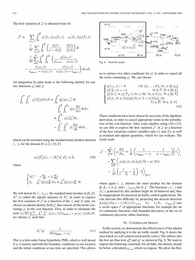
Fig. 8. Network model.

us to enforce two other conditions for in order to cancel allthe terms containing . We can choose

(12)

These conditions have been chosen by necessity of the algebraicderivation, in order to cancel appropriate terms in the perturba-tion of the cost function. After some algebra, using (10)–(12),we are able to express the first variation of as a functionof the first variations control variables only ( and ), as wellas nominal and adjoint quantities, which we can evaluate. Theresult reads

where again denotes the inner product for the domainand for . The functions and

generated by this method might be ill-behaved and, thusbe inappropriate for practical air traffic control applications. Wecan alleviate this difficulty by projecting the descent direction

intoa vector space of appropriate functions, for example the setof continuous functions with bounded derivative, or the set ofcontinuous piecewise affine functions.

VI. CONTROLLER DESIGN

In this section, we demonstrate the effectiveness of the adjointmethod by applying it to the air traffic model. Fig. 8 shows thearea which we will control (enclosed by a box). The inflows intothe box are thus now and as shown in Fig. 8. We want toimpose the following constraint: for all links, the density shouldbe below a threshold which we impose. We allow the flow


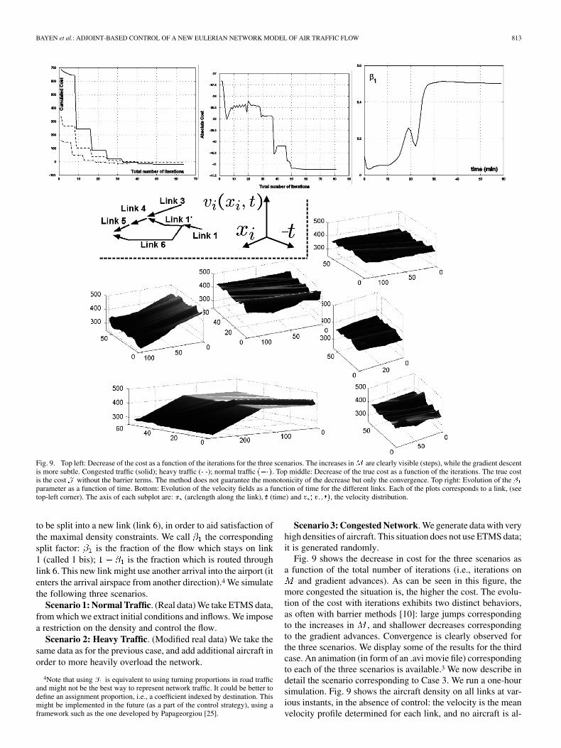
Fig. 9. Top left: Decrease of the cost as a function of the iterations for the three scenarios. The increases in M are clearly visible (steps), while the gradient descentis more subtle. Congested traffic (solid); heavy traffic (- -); normal traffic (��). Top middle: Decrease of the true cost as a function of the iterations. The true costis the cost J without the barrier terms. The method does not guarantee the monotonicity of the decrease but only the convergence. Top right: Evolution of the �parameter as a function of time. Bottom: Evolution of the velocity fields as a function of time for the different links. Each of the plots corresponds to a link, (seetop-left corner). The axis of each subplot are: x (arclength along the link), t (time) and v (x ; t), the velocity distribution.

to be split into a new link (link 6), in order to aid satisfaction ofthe maximal density constraints. We call the correspondingsplit factor: is the fraction of the flow which stays on link1 (called 1 bis); is the fraction which is routed throughlink 6. This new link might use another arrival into the airport (itenters the arrival airspace from another direction).4 We simulatethe following three scenarios.

Scenario 1: Normal Traffic. (Real data) We take ETMS data,from which we extract initial conditions and inflows. We imposea restriction on the density and control the flow.

Scenario 2: Heavy Traffic. (Modified real data) We take thesame data as for the previous case, and add additional aircraft inorder to more heavily overload the network.

4Note that using � is equivalent to using turning proportions in road trafficand might not be the best way to represent network traffic. It could be better todefine an assignment proportion, i.e., a coefficient indexed by destination. Thismight be implemented in the future (as a part of the control strategy), using aframework such as the one developed by Papageorgiou [25].

Scenario 3: Congested Network. We generate data with veryhigh densities of aircraft. This situation does not use ETMS data;it is generated randomly.

Fig. 9 shows the decrease in cost for the three scenarios asa function of the total number of iterations (i.e., iterations on

and gradient advances). As can be seen in this figure, themore congested the situation is, the higher the cost. The evolu-tion of the cost with iterations exhibits two distinct behaviors,as often with barrier methods [10]: large jumps correspondingto the increases in , and shallower decreases correspondingto the gradient advances. Convergence is clearly observed forthe three scenarios. We display some of the results for the thirdcase. An animation (in form of an .avi movie file) correspondingto each of the three scenarios is available.3 We now describe indetail the scenario corresponding to Case 3. We run a one-hoursimulation. Fig. 9 shows the aircraft density on all links at var-ious instants, in the absence of control: the velocity is the meanvelocity profile determined for each link, and no aircraft is al-


Fig. 10. Top 6 subfigures: Evolution of the aircraft density on the different links in the absence of control. Each of the subplot shows the density distribution at agiven time on the corresponding link as in Fig. 9 (the horizontal coordinate represents location, the vertical represents density). The horizontal line represents thedensity threshold (all quantities are nondimensionalized by � , so that the threshold density is 1). As can be seen, the density threshold is violated in link 5 att = 27; t = 39 and t = 59. Bottom 6 subfigures: Evolution of the aircraft density with control applied. Note that link 6 is now open and used. This prevents thesecond violation of density threshold observed in Fig. 10 (t = 59): some of the flow is directly routed from link 1 to link 6. The first violation seen in the top 6subfigures is avoided by speed changes. This figure is also available in form of a .avi file.3

lowed into link 6 (i.e., ). The initial density is shownin the top-left corner. The inflow into links 1 and 3 is such thatat time , the density threshold (represented by the hor-izontal line on each subplot) is violated until time . Attime , it is violated again, until the end of the experiments.Fig. 9 shows the same experiment when link 6 is now openedto traffic, and velocity control is enabled. As can be seen, abouthalf of the traffic incoming into link 1 is rerouted into link 6,and the other half into link 1 bis. Fig. 9 shows the variation of

with time. As can be seen, around min, there is a peakof about 25% of aircraft routed into link 6, which settles to 50%at . The routing control enables avoidance of violation ofmaximal density shown in Fig. 10. The first violation is avoidedby velocity changes.

The velocity profiles are shown in Fig. 9. Each ofthe subplots corresponds to one of the links. For links 5 and 6,one can clearly see the descent velocity profiles. Also, for link6 (subfigure below), one can see a ridge. It corresponds to a setof aircraft which have to fly at high speed into the airport. Onecan also see similar ridges on the other subplots, which havethe same interpretation. For any ridge, the Controller commandcould be to the corresponding set of aircraft: “fly direct at 420 kndirect into [the next waypoint].” Note that in the absence of con-trol, the first violation of the aircraft density threshold occurs33 min after the beginning of the experiment, almost at the endof the network, which is not intuitive. This shows the efficiencyof the method, which is capable of generating the right routingand speed assignments to prevent undesirable events from hap-


Fig. 11. Display of the traffic situation for the static validation. The density ofthe links is depicted by the color. The colored rectangles shown in this plot repre-sent the density. The color scale is: white for zero density; black for highest den-sity. The actual aircraft positions are superimposed (triangles). Traffic is shownat t (top), t + 8min; t + 16min, etc. As can be seen, the peaks of densitycorresponds to the actual positions of the aircraft.

pening much later. Finally, the simulations are also depicted ona U.S. map in Fig. 12. One can see that before , all aircraftchoose the direct route through link 5 to Chicago (it is shorter).After , the excessive amount of flow incoming into links1 and 3 forces the flow to be split through links 1 bis and 6.

The expression of the cost function can be replaced by anyarbitrary user-defined cost as long as the integrand is smooth.The goal of this paper was to prove the feasibility of the tech-nique (with a particular cost function), but extending this to anycost function is a straightforward process (the only thing whichis needed is to recompute the expression of the gradient based onthe new cost, following the steps outlined here). In particular, inthe work of [27], the authors use an integral form with quadraticpenalty. This can be interpreted as penalizing the cumulativedelay minutes at each point in time, and penalizing more se-verely large deviations from the scheduled flow than small ones.

VII. CONCLUSION

We have derived an Eulerian model of the airspace based on amodified LWR partial-differential equation. The network struc-ture of the airspace was modeled as a set of coupled LWR PDEs.Given initial positions of aircraft and airport inflows, this systemof PDEs enables the prediction of the aircraft density. An ana-lytical solution was derived for a single link in the case, in whichthe mean velocity profiles of aircraft along airways do not varywith time (just with space). It can be used for multiple links aswell. ETMS data was used to identify the numerical parame-ters associated with this model. The data is also used to validatethe model, i.e., to demonstrate good predictive capability of thismethod.

We first have shown how to use efficient numerical schemesto simulate the network. We have discarded linear numericalschemes because of their poor performance. We have usedthe Jameson–Schmidt–Turkel scheme as our main numericalscheme to perform numerical simulations of the network.We have posed the problem of maximizing throughput ata destination airport while maintaining the aircraft densitybelow a certain threshold as an optimization program. Theinequality constraints of this program have been handled usinga log-barrier method. The adjoint problem was derived andused to compute the gradient of the augmented cost function.The resulting optimization and control schemes were appliedto a real air traffic case. Simulations show that this methodenables automated control of realistic scenarios as well ashighly congested situations. The output of the code is a set oftime dependent velocity profiles to apply to the network, and apolicy telling how to split the flow in areas of diverging traffic.These outputs could, thus, be used by the Traffic ManagementUnit in charge of managing the flow: they provide high-levelpolicies to apply to the aircraft streams, which are directlyunderstandable by human controllers.

Finally, this formulation of the air traffic flow control problemas an optimization program of PDEs allows for many refine-ments in the control procedure. For instance, gradient descentmay be replaced by more sophisticated optimization methodssuch as approximate Newton method [29] in order to ensurereal time convergence of the algorithm. Furthermore, using thismodel, a decentralized control policy can also be derived using


Fig. 12. Aircraft density in the network around Chicago in presence of control and velocity assignment. The density of the links is depicted by the color. Thecolored rectangles shown in this plot represent the density. The color scale is: white for zero density; black for highest density. As can be seen and was shown inFig. 10, a good portion of the flow is routed into link 6 starting at time t = 51.

decomposition techniques in order to allow different airlinesto separately optimize the flow of their aircraft, while main-taining safety criteria [28]. This method has since been appliedto highway traffic as well [5], [18] and looks promising for otherapplications involving networks of partial differential equations.

VIII. PROOF OF PROPOSITION 1

Existence: is well defined because for all. Its inverse exists because is (strictly) increasing. It

is easy to check that (2) satisfies (1) almost everywhere, and

that it is continuous. This solution has been constructed using atechnique analogous to the algorithm of Bayen and Tomlin [7]based on the method of characteristics.

Uniqueness: Let us call and two continuous weak solu-tions of (1). Call . satisfies:

a.e. in in andin . Multiplying this PDE by and integrating from

to the first discontinuity of gives


from which we deduce

Integrating by parts gives

since and . Using the fact thatfor all . Then,

we use the fact that

so that we can rewrite the inequality as

Using Gronwall’s lemma, this last inequality impliesalmost everywhere in . By continuity,

everywhere in , and, therefore, at . The sameproof applies to since for all .By induction on and are equal everywhere inand, therefore, in .

ACKNOWLEDGMENT

The authors would like to thank Dr. P. K. Menon and Dr.K. Bilimoria for conversations which inspired this work,Dr. G. Chatterji for his ongoing support and suggestions whichwent into modelling this work, and Dr. G. Meyer for his sup-port in this project. They also thank Prof. T. Bewley for usefulconversations regarding the application of the adjoint methodto flow control, and his help in the original formulation of thecontrol problem. Prof. T.-P. Liu helped define the PDE usedfor this model.

REFERENCES

[1] O. M. Aamo and M. Krstic, Flow Control by Feedback. New York:Springer-Verlag, 2002.

[2] R. Ansorge, “What does the entropy condition mean in traffic flowtheory?,” Transp. Res., vol. 24B, no. 2, pp. 133–143, Apr. 1990.

[3] B. Bamieh, F. Paganini, and M. A. Daleh, “Distributed control of spa-tially-invariant systems,” IEEE Trans. Autom. Control, vol. 47, no. 7,pp. 1091–1107, Jul. 2002.

[4] A. M. Bayen, “Computational control of networks of dynamical sys-tems: Application to the National Airspace System,” Ph.D. disserta-tion, Dept. Aeronautics and Astronautics, Stanford Univ., Stanford,CA, 2004.

[5] A. M. Bayen, R. Raffard, and C. J. Tomlin, “Eulerian network model ofair traffic flow in congested areas,” in Proc. Amer. Contr. Conf., 2004,pp. 5520–5526.

[6] A. M. Bayen, R. Raffard, and C. J. Tomlin, “Network congestionalleviation using adjoint hybrid control: Application to highways,”in Number 2993 in Lecture Notes in Computer Science. New York:Springer-Verlag, 2004, pp. 95–110.

[7] A. M. Bayen and C. J. Tomlin, “A construction procedure using char-acteristics for viscosity solutions of the Hamilton-Jacobi equation,” inProc. 40th IEEE Conf. Dec. Contr., 2001, pp. 1657–1662.

[8] T. R. Bewley, “Flow control: New challenges for a new renaissance,”Prog. Aerosp. Sci., vol. 37, no. 1, pp. 1–119, Jan. 2001.

[9] K. Bilimoria, B. Sridhar, G. Chatterji, K. Seth, and S. Graabe, “FACET:Future ATM concepts evaluation tool,” in Proc. 3rd USA/Eur. AirTraffic Manage. R&D Seminar, 2001, on CDROM.

[10] S. Boyd and L. Vandenberghe, Convex Optimization. Cambridge,U.K.: Cambridge Univ. Press, 2004.

[11] G. Chatterji, B. Sridhar, and D. Kim, “Analysis of ETMS data qualiy fortraffic flow management decisions,” in Proc. AIAA Conf. Guid., Nav.Contr., 2003, AIAA-2003-5626.

[12] C. Chen, Z. Jia, and P. Varaiya, “Causes and cures of highwaycongestion,” IEEE Control Syst. Mag., vol. 21, no. 4, pp. 26–33,Dec. 2001.

[13] P. D. Christofides, Nonlinear and Robust Control of Partial DifferentialEquation Systems: Methods and Applications to Transport-ReactionProcesses. Cambridge, MA: Birkhäuser, 2001.

[14] C. Daganzo, “The cell transmission model: A dynamic representationof highway traffic consistent with the hydrodynamic theory,” Trans-port. Res., vol. 28B, no. 4, pp. 269–287, Aug. 1994.

[15] C. Daganzo, “The cell transmission model, Part II: Network traffic,”Transport. Res., vol. 29B, no. 2, pp. 79–93, Apr. 1995.

[16] C. Daganzo, “A finite difference approximation of the kinematic wavemodel of traffic flow,” Transport. Res., vol. 29B, no. 4, pp. 261–276,Aug. 1995.

[17] C. Hirsch, Numerical Computation of Internal and External Flows.New York: Wiley, 1988.

[18] D. Jacquet, C. Canudas de Wit, and D. Koenig, “Optimal ramp meteringstrategy with an extended LWR model: Analysis and computationalmethods,” in Proc. 16th IFAC World Congr., 2005, to be published.

[19] A. Jameson, “Aerodynamic design via control theory,” J. ScientificComput., vol. 3, no. 3, pp. 233–260, Sep. 1988.

[20] A. Jameson, “Analysis and design of numerical schemes for gas dy-namics 1: Artificial diffusion, upwind biasing, limiters and their effecton accuracy and multigrid convergence,” Int. J. Computational FluidDyn., vol. 4, pp. 171–218, Sep. 1995.

[21] M. Krstic, “On global stabilization of Burgers’ equation by boundarycontrol,” Syst. Control Lett., vol. 37, pp. 123–142, Jul. 1999.

[22] M. J. Lighthill and G. B. Whitham, “On kinematic waves. II. A theoryof traffic flow on long crowded roads,” in Proc. Royal Soc. London,1956, pp. 317–345.

[23] X. Litrico, “Robust IMC flow control of SIMO dam-river open-channelsystems,” IEEE Trans. Control Syst. Technol., vol. 10, no. 5, pp.432–437, May 2002.

[24] P. K. Menon, G. D. Sweriduk, and K. Bilimoria, “New approach formodeling, analysis, and control of air traffic flow,” AIAA J. Guid.,Contr., Dyn., vol. 27, no. 5, pp. 731–5090, Sep./Oct. 2004.

[25] A. Messmer and M. Papageorgiou, “Route diversion control in mo-torway networks via nonlinear optimization,” IEEE Trans. ControlSyst. Technol., vol. 3, no. 1, pp. 144–154, Mar. 1995.

[26] L. Munoz, X. Sun, R. Horowitz, and L. Alvarez, “Traffic density esti-mation with the cell transmission model,” in Proc. Amer. Contr. Conf.,2003, pp. 3750–3755.

[27] R. Raffard, S. L. Waslander, A. M. Bayen, and C. J. Tomlin, “Towardefficient and equitable distributed air traffic flow control,” presented atthe Proc. Amer. Contr. Conf., 2006, Minneapolis, MN.

[28] R. Raffard, S. L. Waslander, A. M. Bayen, and C. J. Tomlin, “A co-operative, distributed approach to multi-agent Eulerian network con-trol: Application to air traffic management,” in Proc. AIAA Guid., Nav.Contr. Conf. Exhibit, 2005, AIAA-2005-6050.

[29] R. L. Raffard and C. J. Tomlin, “Second order optimization of ordinaryand partial differential equations with applications to air traffic flow,”in Proc. Amer. Contr. Conf., 2005, pp. 798–803.

[30] P. I. Richards, “Shock waves on the highway,” Oper. Res., vol. 4, no.1, pp. 42–51, Feb. 1956.

[31] C. Robelin, D. Sun, G. Wu, and A. M. Bayen, “En-route air trafficmodeling and strategic flow management using mixed integer linearprogramming,” in INFORMS Annu. Meeting, 2005.

[32] R. C. Smith and M. A. Demetriou, Research Directions in DistributedParameter Systems. Philadelphia, PA: SIAM, 2000.


[33] D. Sun, S. Yang, I. S. Strub, B. Sridhar, K. Sheth, and A. M. Bayen,“Assessment of the respective performance of three Eulerian air trafficflow models,” presented at the Proc. AIAA Conf. Guid., Nav. Contr.,Keystone, CO, 2006.

[34] Y. Wang, M. Papageorgiou, and A. Messmer, “Motorway traffic stateestimation based on extended Kalman filter,” in Proc. Euro. Contr.Conf., 2003.

Alexandre M. Bayen (S’02–M’04) received the B.S.degree in applied mathematics from the Ecole Poly-technique, Palaiseau, France, in 1998, the M .S. andPh.D. degrees in aeronautics and astronautics fromStanford University, Stanford, CA, in 1999 and 2004,respectively.

He was a Visiting Researcher at NASA Ames,Moffett Field, CA, from 2001 to 2003. From 2004to 2005, he worked for the Department of Defense,France, where he held the rank of Major. During thattime, he was the Research Director of the Labora-

toire de Navigation Autonome at the Laboratoire de Recherches Balistiques etAérodynamiques, Vernon, France. Since March 2005, he has been an AssistantProfessor in the Department of Civil and Environmental Engineering at theUniversity of California at Berkeley, Berkeley. His research interests includecontrol of distributed parameter systems, combinatorial optimization, hybridsystems, and air traffic automation.

Dr. Bayen is a recipient of the Graduate Fellowship of the DélégationGénérale pour l’Armement (1998–2002) from France, and the Ballhaus Prizefor best doctoral thesis from the Department of Aeronautics and Astronauticsat Stanford University (2004).

Robin L. Raffard received the M.S. degree in me-chanical engineering from the Ecole Centrale Paris,France, in 2002, and the M.S. degree in aeronauticsand astronautics from Stanford University, Stanford,CA, in 2003. He is currently working towards thePh.D. degree in aeronautics and astronautics at thesame school.

His research interests include distributed opti-mization and optimal control of systems governedby differential equations, with applications in airtraffic flow, systems biology, and stochastic systems.

Claire J. Tomlin (S’93–M’99) received the Ph.D.degree in electrical engineering from the Universityof California at Berkeley, Berkeley, in 1998. She alsoreceived the M.Sc. degree from Imperial College,London, in 1993, and the B.A.Sc. degree from theUniversity of Waterloo, Canada, in 1992, both inelectrical engineering.

She is an Associate Professor in the Department ofElectrical Engineering and Computer Sciences at theUniversity of California at Berkeley, and is an As-sociate Professor in the Department of Aeronautics

and Astronautics at Stanford University, Stanford, CA, where she also holds theVance D. and Arlene C. Coffman Faculty Scholarship in the School of Engi-neering. She joined Stanford in September 1998, as a Terman Assistant Pro-fessor, and received tenure at Stanford in November 2004. In July 2005, shejoined Berkeley as an Associate Professor. She has held visiting research po-sitions at NASA Ames, Honeywell Labs, and the University of British Co-lumbia. Her research interests include control systems, specifically hybrid con-trol theory, and she works on air traffic control automation, flight managementsystem analysis and design, and modeling and analysis of biological cell net-works.

Dr. Tomlin is a recipient of the Eckman Award of the American AutomaticControl Council (2003), MIT Technology Review’s Top 100 Young InnovatorsAward (2003), the AIAA Outstanding Teacher Award (2001), an National Sci-ence Foundation (NSF) Career Award (1999), and the Bernard Friedman Memo-rial Prize in Applied Mathematics (1998).

804 ieee transactions on control systems …tomlin/papers/journals/brt06_tcst.pdf · 804 ieee...

Documents