spat ial tree algorithms

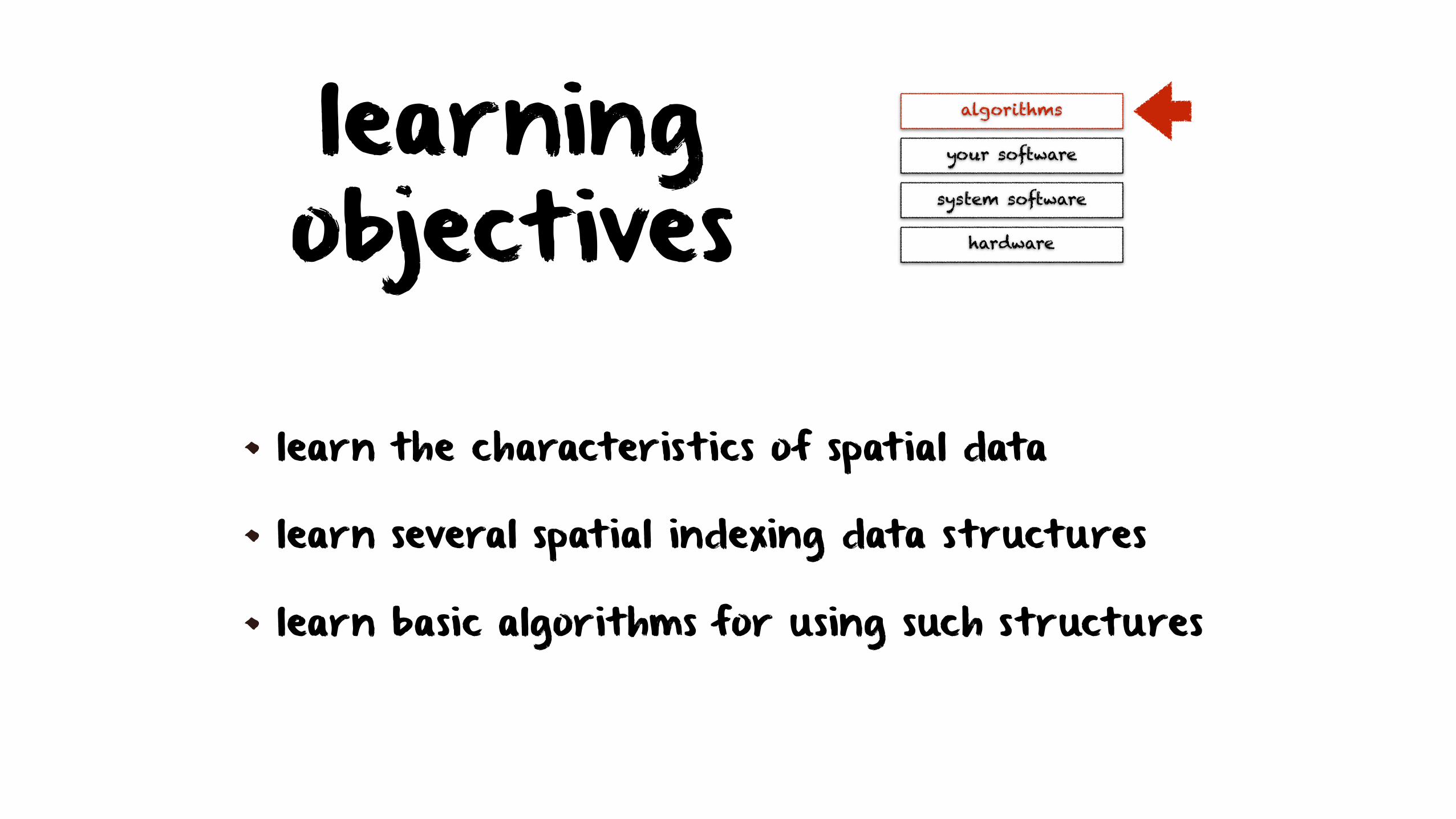
learning objectives

learn the characteristics of spatial data

learn several spatial indexing data structures

learn basic algorithms for using such structures

hardware

your software

algorithms

system software

geographic information systems, e.g.,location search & route planning

mathematical visualization, e.g., proofwithout words, mandelbrot set s, etc.

z 7! zd + ca2 + b2 = c2

development made possible by exponential progress in computer graphics, with multiple applications

a branch of computer science focusing on data structures & algorithms for

solving geometric problems

computational geometry

computer-aided engineering,e.g., mechanical design

computer vision e.g., 3D graphics

in games

with 1-dimensional data, natural ordering implicitly partitions the data, e.g., binary tree

with 1-dimensional data, the static case is rather simple and solved by sorting the data

spatial data is intrinsically multidimensional, so thereis no natural ordering of data (e.g., of points)

computational geometrywhat’s specific to spatial data?

with multidimensional data, the static case is far from simple and solved by several partitioning techniques

computational geometry

x

y

range queries: given a set of point s P, find the points contained within a given rectangle

intersection queries: given a set of rectangles R, find which rectangles intersect a target rectangle

collision detection: given a set of shapes S, find the intersections between all these shapes

nearest neighbor: given a set of point s P, find which one is closest to a target point pt

typical problems

computational geometrybrute-force algorithm

nearest neighbor: given a set of points P, find which one is closest to a target point pt

NEAREST–NEIGHBOR (P, pt) p ⟵ NIL min ⟵ ∞ for each pi ∈ P if distance( pi, pt) < min min ⟵ distance( pi, pt) p ⟵ pi

return ( p, min)Complexity: O(n), with n = |P|

spatial tree structures

Complexity: O(log n), with n = |P|

they index spatial object s

quad-trees

R-trees

kd-trees

typical approaches

a recursive tree, where each node has between M and mmmmm children, except for the root which has at least two

m =

�M2

⌫

all leaves are at the same level, i.e., the tree is height balanced

only leaf nodes contain actual spatial object entries, each consisting of the spatial object it self and a minimum bounding region (mbr)

containing that object, i.e., object = (shape, mbr)

internal nodes contain children entries, each consisting of a link to the child node and an mbr covering all children nodes of that child, i.e., node = (child, mbr)

an minimum bounding region is typically of the form mbr = (xmin, ymin, xmax, ymax)

R-tree A. Guttman. R-trees: A dynamic index structure for spatial searching. In Proceedings of the 1984 ACM SIGMOD International Conference on

Management of Data, pages 47–57, New York, NY, USA, 1984. ACM.

6

9

5

4

78

3

1

2

only leaf nodes contain actual spatial object entries, each consisting of the spatial object it self and a minimum bounding region (mbr)

containing that object, i.e., object = (shape, mbr)

R5

R4

R3

R-tree

R6

R2

R1

96 4 5 1 2 3 7 8

R1 R2

R3 R4 R5 R6

root

root

important: the root also contains a minimum bounding box

internal nodes contain children entries, each consisting of a link to the child node and an mbr covering all children nodes

of that child, i.e., node = (child, mbr)

important: the root also contains a minimum bounding box

INTERSECT (node, region) if node.mbr ⊂ region return { object | object ∈ REACHABLE-LEAVES(node) } if node is a leaf return { object ∈ node | object.mbr ∩ region ≠ ∅ } result ⟵ ∅ for each kid ∈ node.children if kid.mbr ∩ region ≠ ∅ result = result ∪ INTERSECT (kid.child, region) return result

SEARCH (node, shape) if node is a leaf if ∃object ∈ node : object.shape = shape return object return NIL for each kid ∈ node.children if shape.mbr ⊆ kid.mbr return SEARCH(kid.child, shape) return NIL

R-tree

96 4 5 1 2 3 7 8

R1 R2

R3 R4 R5 R6

root

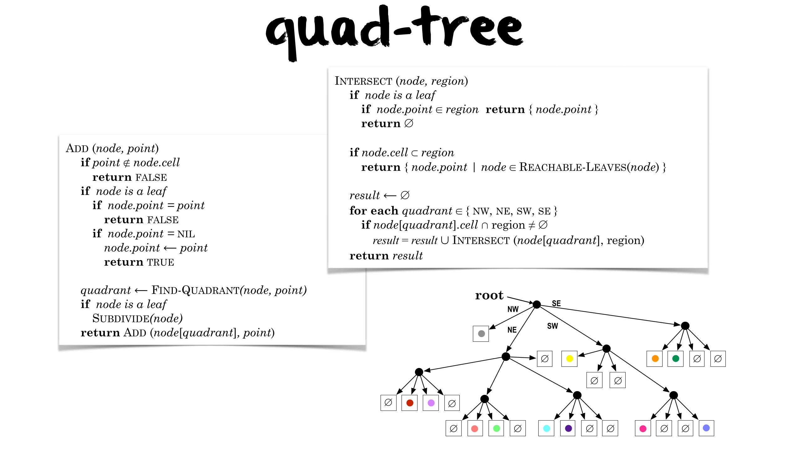
a recursive tree where each internal node has four children

quad-tree R. A. Finkel and J. L. Bentley. Quad trees a data structure for retrieval on composite

keys. Acta Informatica, 4(1):1–9, 1974.

like R-trees, only leaf nodes store actual geometrical object s

predefined partitioning with subcells (quadrants) named asNorth West (NW), North-East (NE), South-West (SW) and South-East (SE)

each node represents a cell in the geometrical space, with it s children partitioning that cell into an equally sized subcell

AB

C D

F E

G H

J

K

I

LM

R

S T

UV W

XY

O N

QP

rootNW

NE SW

SE

R

F E G H

B A C D J I K L V W X Y

M S

T U

O N P Q

NW

NE SW

SE

quad-treeroot

NW

NE SW

SE

0

0 1 0 1

1 1 0 0 1 1 1 0 1 1 0 0

0 1

0 0

1 0 1 0

root

∅ ∅

∅ ∅

∅

∅ ∅

∅ ∅

∅ ∅

∅ ∅

region quad-tree

point-region quad-tree

quad-tree

root

ADD (node, point) if point ∉ node.cell return FALSE if node is a leaf if node.point = point return FALSE if node.point = NIL node.point ⟵ point return TRUE

quadrant ⟵ FIND-QUADRANT(node, point) if node is a leaf SUBDIVIDE(node) return ADD (node[quadrant], point)

quad-tree

NW

NE SW

SE

INTERSECT (node, region) if node is a leaf if node.point ∈ region return { node.point } return ∅

if node.cell ⊂ region return { node.point | node ∈ REACHABLE-LEAVES(node) } result ⟵ ∅ for each quadrant ∈ { NW, NE, SW, SE } if node[quadrant].cell ∩ region ≠ ∅ result = result ∪ INTERSECT (node[quadrant], region) return result

∅ ∅

∅ ∅

∅

∅ ∅

∅ ∅

∅ ∅

∅ ∅

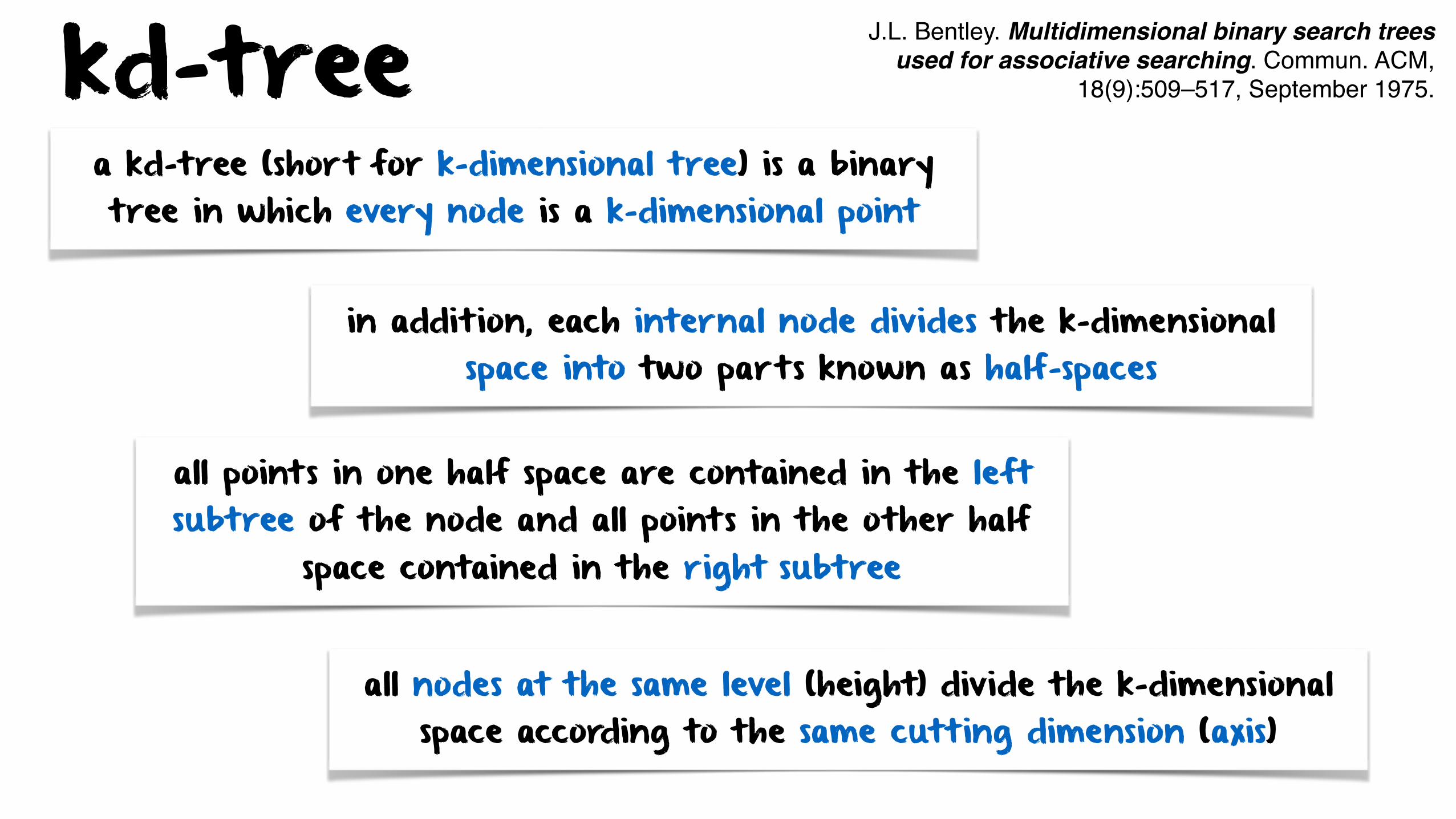
kd-tree J.L. Bentley. Multidimensional binary search trees used for associative searching. Commun. ACM,

18(9):509–517, September 1975.

in addition, each internal node divides the k-dimensional space into two parts known as half-spaces

a kd-tree (short for k-dimensional tree) is a binary tree in which every node is a k-dimensional point

all points in one half space are contained in the left subtree of the node and all points in the other half

space contained in the right subtree

all nodes at the same level (height) divide the k-dimensional space according to the same cutting dimension (axis)

k-d-tree1

8

3

105

4

2

9

6

7

ADD (node, point, cutaxis) if node = NIL node ⟵ CREATE-NODE node.point = point return node if point[cutaxis] ≤ node.point[cutaxis] node.left = ADD(node.left, point, (cutaxis + 1) mod k) else node.right = ADD(node.right, point, (cutaxis + 1) mod k) return node

1

32

54 87

6 9 10

x-axis

y-axis

x-axis

y-axisRemarks

• Points are stored as k-dimensional arrays

• Each axis corresponds to an index: ‣ x-axis corresponds to index 0 ‣ y-axis corresponds to index 1 ‣ etc...

• So assuming point pi = (xi,yi) = (3,7),we have that pi = [3,7], xi = p[0] = 7 and yi = p[1] = 7

• In this example, initially root = NIL and points are inserted as follows: ‣ ADD(root,p1, 0) ‣ ADD(root,p2, 0) ‣ ADD(root,p3, 0) ‣ etc...

root