8 interpretation of survey results 8.1 … · 8 interpretation of survey results ... adequate, but...

8 INTERPRETATI ON OF SURVEY RESULTS

8.1 Introduction

This chapter discusses the interpretation of survey results, primarily those of the final status survey. Interpreting a survey’s results is most straightforward when measurement data are entirely higher or lower than the DCGLW. In such cases, the decision that a survey unit meets or exceeds the release criterion requires little in terms of data analysis. However, formal statistical tests provide a valuable tool when a survey unit’s measurements are neither clearly above nor entirely below the DCGLW. Nevertheless, the survey design always makes use of the statistical tests in helping to assure that the number of sampling points and the measurement sensitivity are adequate, but not excessive, for the decision to be made.

Section 8.2 discusses the assessment of data quality. The remainder of this chapter deals with application of the statistical tests used in the decision-making process, and the evaluation of the test results. In addition, an example checklist is provided to assist the user in obtaining the necessary information for interpreting the results of a final status survey.

8.2 Data Quality Assessment

Data Quality Assessment (DQA) is a scientific and statistical evaluation that determines if the data are of the right type, quality, and quantity to support their intended use. An overview of the DQA process appears in Section 2.3 and Appendix E. There are five steps in the DQA process:

! Review the Data Quality Objectives (DQOs) and Survey Design

! Conduct a Preliminary Data Review

! Select the Statistical Test

! Verify the Assumptions of the Statistical Test

! Draw Conclusions from the Data

The effort expended during the DQA evaluation should be consistent with the graded approach used in developing the survey design. More information on DQA is located in Appendix E, and the EPA Guidance Document QA/G-9 (EPA 1996a). Data should be verified and validated as described in Section 9.3 prior to the DQA evaluation.

August 2000 8-1 MARSSIM, Revision 1

Interpretation of Survey Results

8.2.1 Review the Data Quality Objectives (DQOs) and Sampling Design

The first step in the DQA evaluation is a review of the DQO outputs to ensure that they are still applicable. For example, if the data suggest the survey unit was misclassified as Class 3 instead of Class 1, then the original DQOs should be redeveloped for the correct classification.

The sampling design and data collection documentation should be reviewed for consistency with the DQOs. For example, the review should check that the appropriate number of samples were taken in the correct locations and that they were analyzed with measurement systems with appropriate sensitivity. Example checklists for different types of surveys are given in Chapter 5.

Determining that the sampling design provides adequate power is important to decision making, particularly in cases where the levels of residual radioactivity are near the DCGLW. This can be done both prospectively, during survey design to test the efficacy of a proposed design, and retrospectively, during interpretation of survey results to determine that the objectives of the design are met. The procedure for generating power curves for specific tests is discussed in Appendix I. Note that the accuracy of a prospective power curve depends on estimates of the data variability, �, and the number of measurements. After the data are analyzed, a sample estimate of the data variability, namely the sample standard deviation (s) and the actual number of valid measurements will be known. The consequence of inadequate power is that a survey unit that actually meets the release criterion has a higher probability of being incorrectly deemed not to meet the release criterion.

8.2.2 Conduct a Preliminary Data Review

To learn about the structure of the data—identifying patterns, relationships, or potential anomalies—one can review quality assurance (QA) and quality control (QC) reports, prepare graphs of the data, and calculate basic statistical quantities.

8.2.2.1 Data Evaluation and Conversion

Radiological survey data are usually obtained in units, such as the number of counts per unit time, that have no intrinsic meaning relative to DCGLs. For comparison of survey data to DCGLs, the survey data from field and laboratory measurements are converted to DCGL units. Further information on instrument calibration and data conversion is given in Section 6.2.7.

Basic statistical quantities that should be calculated for the sample data set are the:

! mean ! standard deviation ! median

MARSSIM, Revision 1 8-2 August 2000


Example:

Suppose the following 20 concentration values are from a survey unit:

90.7, 83.5, 86.4, 88.5, 84.4, 74.2, 84.1, 87.6, 78.2, 77.6, 86.4, 76.3, 86.5, 77.4, 90.3, 90.1, 79.1, 92.4, 75.5, 80.5.

First, the average of the data (83.5) and the sample standard deviation (5.7) should be calculated.

The average of the data can be compared to the reference area average and the DCGLW to get a preliminary indication of the survey unit status. Where remediation is inadequate, this comparison may readily reveal that a survey unit contains excess residual radioactivity—even before applying statistical tests. For example, if the average of the data exceeds the DCGLW and the radionuclide of interest does not appear in background, then the survey unit clearly does not meet the release criterion. On the other hand, if every measurement in the survey unit is below the DCGLW, the survey unit clearly meets the release criterion.1

The value of the sample standard deviation is especially important. If too large compared to that assumed during the survey design, this may indicate an insufficient number of samples were collected to achieve the desired power of the statistical test. Again, inadequate power can lead to unnecessary remediation.

The median is the middle value of the data set when the number of data points is odd, and is the average of the two middle values when the number of data points is even. Thus 50% of the data points are above the median, and 50% are below the median. Large differences between the mean and the median would be an early indication of skewness in the data. This would also be evident in a histogram of the data. For the example data above, the median is 84.25 (i.e., (84.1 + 84.4)/2). The difference between the median and the mean (i.e., 84.25 - 83.5 = 0.75) is a small fraction of the sample standard deviation (i.e., 5.7). Thus, in this instance, the mean and median would not be considered significantly different.

Examining the minimum, maximum, and range of the data may provide additional useful information. The minimum in this example is 74.2 and the maximum is 92.4, so the range is 92.4 - 74.2 = 18.2. This is only 3.2 standard deviations. Thus, the range is not unusually large. When there are 30 or fewer data points, values of the range much larger than about 4 to 5 standard deviations would be unusual. For larger data sets the range might be wider.

1 It can be verified that if every measurement is below the DCGLW, the conclusion from the statistical tests will always be that the survey unit does not exceed the release criterion.



8.2.2.2 Graphical Data Review

At a minimum, a graphical data review should consist of a posting plot and a histogram. Quantile plots are also useful diagnostic tools, particularly in the two-sample case, to compare the survey unit and reference area. These are discussed in Appendix I, Section I.8.

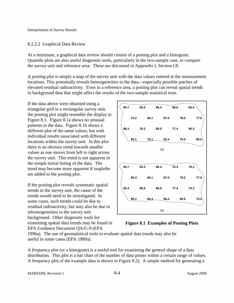
A posting plot is simply a map of the survey unit with the data values entered at the measurement locations. This potentially reveals heterogeneities in the data—especially possible patches of elevated residual radioactivity. Even in a reference area, a posting plot can reveal spatial trends in background data that might affect the results of the two-sample statistical tests.

If the data above were obtained using a triangular grid in a rectangular survey unit, the posting plot might resemble the display in Figure 8.1. Figure 8.1a shows no unusual patterns in the data. Figure 8.1b shows a different plot of the same values, but with individual results associated with different locations within the survey unit. In this plot there is an obvious trend towards smaller values as one moves from left to right across the survey unit. This trend is not apparent in the simple initial listing of the data. The trend may become more apparent if isopleths are added to the posting plot.

If the posting plot reveals systematic spatial trends in the survey unit, the cause of the trends would need to be investigated. In some cases, such trends could be due to residual radioactivity, but may also be due to inhomogeneities in the survey unit background. Other diagnostic tools for examining spatial data trends may be found in EPA Guidance Document QA/G-9 (EPA

90.7 83.5 86.4 88.5 84.4

74.2 84.1 87.6 78.2 77.6

86.4 76.3 86.5 77.4 90.3

90.1 79.1 92.4 75.5 80.5

(a)

90.7 83.5 86.4 76.3 79.1

90.3 84.1 87.6 78.2 77.6

92.4 88.5 86.5 77.4 74.2

90.1 84.4 86.4 80.5 75.5

(b)

Figure 8.1 Examples of Posting Plots

1996a). The use of geostatistical tools to evaluate spatial data trends may also be useful in some cases (EPA 1989a).

A frequency plot (or a histogram) is a useful tool for examining the general shape of a data distribution. This plot is a bar chart of the number of data points within a certain range of values. A frequency plot of the example data is shown in Figure 8.2). A simple method for generating a



8-5August 2000 MARSSIM, Revision 1

Figure 8.2 ple of a Frequency Plot

rough frequency plot is the stem and leaf display discussed in Appendix I, Section I.7. frequency plot will reveal any obvious departures from symmetry, such as skewness orbimodality (two peaks), in the data distributions for the survey unit or reference area. Thepresence of two peaks in the survey unit frequency plot may indicate the existence of isolatedareas of residual radioactivity. n some cases it may be possible to determine an appropriatebackground for the survey unit using this information. purpose will generally be highly dependent on site-specific considerations and should only bepursued after a consultation with the responsible regulatory agency.

The presence of two peaks in the background reference area or survey unit frequency plot mayindicate a mixture of background concentration distributions due to different soil types,construction materials, etc. The greater variability in the data due to the presence of such amixture will reduce the power of the statistical tests to detect an adequately remediated surveyunit. carefully matching thebackground reference areas to the survey units, and choosing survey units with homogeneousbackgrounds.

Skewness or other asymmetry can impact the accuracy of the statistical tests. atransformation (e.g., taking the logarithms of the data) can sometimes be used to make thedistribution more symmetric. data. hen the underlying data distribution is highly skewed, it is often because there are a fewhigh areas. ince the EMC is used to detect such measurements, the difference between usingthe median and the mean as a measure for the degree to which uniform residual radioactivityremains in a survey unit tends to diminish in importance.

Exam

The

IThe interpretation of the data for this

These situations should be avoided whenever possible by

A dat

The statistical tests would then be performed on the transformedW

S


8.2.3 Select the Tests

An overview of the statistical considerations important for final status surveys appears in Section 2.5 and Appendix D. The most appropriate procedure for summarizing and analyzing the data is chosen based on the preliminary data review. The parameter of interest is the mean concentration in the survey unit. The nonparametric tests recommended in this manual, in their most general form, are tests of the median. If one assumes that the data are from a symmetric distribution—where the median and the mean are effectively equal—these are also tests of the mean. If the assumption of symmetry is violated, then nonparametric tests of the median approximately test the mean. Computer simulations (e.g., Hardin and Gilbert, 1993) have shown that the approximation is a good one. That is, the correct decision will be made about whether or not the mean concentration exceeds the DCGL, even when the data come from a skewed distribution. In this regard, the nonparametric tests are found to be correct more often than the commonly used Student’s t test. The robust performance of the Sign and WRS tests over a wide range of conditions is the reason that they are recommended in this manual.

When a given set of assumptions is true, a parametric test designed for exactly that set of conditions will have the highest power. For example, if the data are from a normal distribution, the Student’s t test will have higher power than the nonparametric tests. It should be noted that for large enough sample sizes (e.g., large number of measurements), the Student’s t test is not a great deal more powerful than the nonparametric tests. On the other hand, when the assumption of normality is violated, the nonparametric tests can be very much more powerful than the t test. Therefore, any statistical test may be used provided that the data are consistent with the assumptions underlying their use. When these assumptions are violated, the prudent approach is to use the nonparametric tests which generally involve fewer assumptions than their parametric equivalents.

The one-sample statistical test (Sign test) described in Section 5.5.2.3 should only be used if the contaminant is not present in background and radionuclide-specific measurements are made. The one-sample test may also be used if the contaminant is present at such a small fraction of the DCGLW value as to be considered insignificant. In this case, background concentrations of the radionuclide are included with the residual radioactivity (i.e., the entire amount is attributed to facility operations). Thus, the total concentration of the radionuclide is compared to the release criterion. This option should only be used if one expects that ignoring the background concentration will not affect the outcome of the statistical tests. The advantage of ignoring a small background contribution is that no reference area is needed. This can simplify the final status survey considerably.

The one-sample Sign test (Section 8.3.1) evaluates whether the median of the data is above or

W. If the data distribution is symmetric, the median is equal to the mean. In cases where the data are severely skewed, the mean may be above the DCGLbelow the DCGL

W, while the median



is below the DCGLW. In such cases, the survey unit does not meet the release criterion regardless of the result of the statistical tests. On the other hand, if the largest measurement is below the DCGLW, the Sign test will always show that the survey unit meets the release criterion.

For final status surveys, the two-sample statistical test (Wilcoxon Rank Sum test, discussed in Section 5.5.2.2) should be used when the radionuclide of concern appears in background or if measurements are used that are not radionuclide specific. The two-sample Wilcoxon Rank Sum (WRS) test (Section 8.4.1) assumes the reference area and survey unit data distributions are similar except for a possible shift in the medians. When the data are severely skewed, the value for the mean difference may be above the DCGLW, while the median difference is below the DCGLW. In such cases, the survey unit does not meet the release criterion regardless of the result of the statistical test. On the other hand, if the difference between the largest survey unit measurement and the smallest reference area measurement is less than the DCGLW, the WRS test will always show that the survey unit meets the release criterion.

8.2.4 Verif y the Assumptions of the Tests

An evaluation to determine that the data are consistent with the underlying assumptions made for the statistical procedures helps to validate the use of a test. One may also determine that certain departures from these assumptions are acceptable when given the actual data and other information about the study. The nonparametric tests described in this chapter assume that the data from the reference area or survey unit consist of independent samples from each distribution.

Spatial dependencies that potentially affect the assumptions can be assessed using posting plots (Section 8.2.2.2). More sophisticated tools for determining the extent of spatial dependencies are also available (e.g., EPA QA/G-9). These methods tend to be complex and are best used with guidance from a professional statistician.

Asymmetry in the data can be diagnosed with a stem and leaf display, a histogram, or a Quantile plot. As discussed in the previous section, data transformations can sometimes be used to minimize the effects of asymmetry.

One of the primary advantages of the nonparametric tests used in this report is that they involve fewer assumptions about the data than their parametric counterparts. If parametric tests are used, (e.g., Student’s t test), then any additional assumptions made in using them should be verified (e.g., testing for normality). These issues are discussed in detail in EPA QA/G-9 (EPA 1996a).



One of the more important assumptions made in the survey design described in Chapter 5 is that the sample sizes determined for the tests are sufficient to achieve the data quality objectives set for the Type I (�) and Type II (�) error rates. Verification of the power of the tests (1-�) to detect adequate remediation may be of particular interest. Methods for assessing the power are discussed in Appendix I.9. If the hypothesis that the survey unit residual radioactivity exceeds the release criterion is accepted, there should be reasonable assurance that the test is equally effective in determining that a survey unit has residual contamination less than the DCGLW. Otherwise, unnecessary remediation may result. For this reason, it is better to plan the surveys cautiously—even to the point of:

! overestimating the potential data variability ! taking too many samples ! overestimating minimum detectable concentrations (MDCs)

If one is unable to show that the DQOs were met with reasonable assurance, a resurvey may be needed. Examples of assumptions and possible methods for their assessment are summarized in Table 8.1.

Table 8.1 Methods for Checking the Assumptions of Statistical Tests

Assumption Diagnostic

Spatial Independence Posting Plot

Symmetry Histogram, Quantile Plot

Data Variance Sample Standard Deviation

Power is Adequate Retrospective Power Chart

8.2.5 Draw Conclusions from the Data

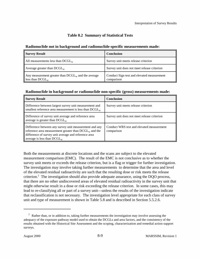
The types of measurements that can be made in a survey unit are 1) direct measurements at discrete locations, 2) samples collected at discrete locations, and 3) scans. The statistical tests are only applied to measurements made at discrete locations. Specific details for conducting the statistical tests are given in Sections 8.3 and 8.4. When the data clearly show that a survey unit meets or exceeds the release criterion, the result is often obvious without performing the formal statistical analysis. Table 8.2 describes examples of circumstances leading to specific conclusions based on a simple examination of the data.



Table 8.2 Summary of Statistical Tests

Radionuclide not in background and radionuclide-specific measurements made:

Survey Result Conclusion

All measurements less than DCGLW Survey unit meets release criterion

Average greater than DCGLW Survey unit does not meet release criterion

Any measurement greater than DCGLW and the average less than DCGLW

Conduct Sign test and elevated measurement comparison

Radionuclide in background or radionuclide non-specific (gross) measurements made:

Survey Result Conclusion

Difference between largest survey unit measurement and smallest reference area measurement is less than DCGLW

Survey unit meets release criterion

Difference of survey unit average and reference area average is greater than DCGLW

Survey unit does not meet release criterion

Difference between any survey unit measurement and any reference area measurement greater than DCGLW and the difference of survey unit average and reference area average is less than DCGLW

Conduct WRS test and elevated measurement comparison

Both the measurements at discrete locations and the scans are subject to the elevated measurement comparison (EMC). The result of the EMC is not conclusive as to whether the survey unit meets or exceeds the release criterion, but is a flag or trigger for further investigation. The investigation may involve taking further measurements to determine that the area and level of the elevated residual radioactivity are such that the resulting dose or risk meets the release criterion.2 The investigation should also provide adequate assurance, using the DQO process, that there are no other undiscovered areas of elevated residual radioactivity in the survey unit that might otherwise result in a dose or risk exceeding the release criterion. In some cases, this may lead to re-classifying all or part of a survey unit—unless the results of the investigation indicate that reclassification is not necessary. The investigation level appropriate for each class of survey unit and type of measurement is shown in Table 5.8 and is described in Section 5.5.2.6.

2 Rather than, or in addition to, taking further measurements the investigation may involve assessing the adequacy of the exposure pathway model used to obtain the DCGLs and area factors, and the consistency of the results obtained with the Historical Site Assessment and the scoping, characterization and remedial action support surveys.



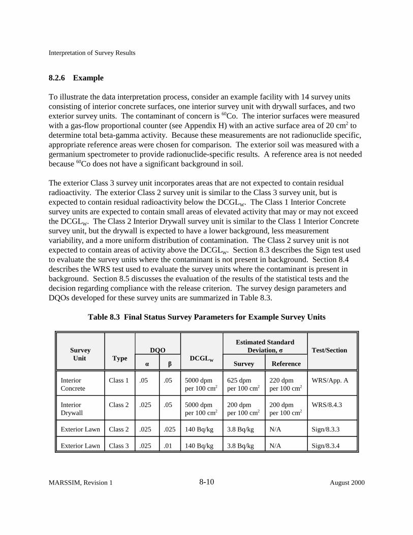
8.2.6 Example

To illustrate the data interpretation process, consider an example facility with 14 survey units consisting of interior concrete surfaces, one interior survey unit with drywall surfaces, and two exterior survey units. The contaminant of concern is 60Co. The interior surfaces were measured with a gas-flow proportional counter (see Appendix H) with an active surface area of 20 cm2 to determine total beta-gamma activity. Because these measurements are not radionuclide specific, appropriate reference areas were chosen for comparison. The exterior soil was measured with a germanium spectrometer to provide radionuclide-specific results. A reference area is not needed because 60Co does not have a significant background in soil.

The exterior Class 3 survey unit incorporates areas that are not expected to contain residual radioactivity. The exterior Class 2 survey unit is similar to the Class 3 survey unit, but is expected to contain residual radioactivity below the DCGLW. The Class 1 Interior Concrete survey units are expected to contain small areas of elevated activity that may or may not exceed the DCGLW. The Class 2 Interior Drywall survey unit is similar to the Class 1 Interior Concrete survey unit, but the drywall is expected to have a lower background, less measurement variability, and a more uniform distribution of contamination. The Class 2 survey unit is not expected to contain areas of activity above the DCGLW. Section 8.3 describes the Sign test used to evaluate the survey units where the contaminant is not present in background. Section 8.4 describes the WRS test used to evaluate the survey units where the contaminant is present in background. Section 8.5 discusses the evaluation of the results of the statistical tests and the decision regarding compliance with the release criterion. The survey design parameters and DQOs developed for these survey units are summarized in Table 8.3.

Table 8.3 Final Status Survey Parameters for Example Survey Units

Survey Unit Type

DQO DCGL W

Estimated Standard Deviation, � Test/Section

� � Survey Reference

Interior Concrete

Class 1 .05 .05 5000 dpm per 100 cm2

625 dpm per 100 cm2

220 dpm per 100 cm2

WRS/App. A

Interior Drywall

Class 2 .025 .05 5000 dpm per 100 cm2

200 dpm per 100 cm2

200 dpm per 100 cm2

WRS/8.4.3

Exterior Lawn Class 2 .025 .025 140 Bq/kg 3.8 Bq/kg N/A Sign/8.3.3

Exterior Lawn Class 3 .025 .01 140 Bq/kg 3.8 Bq/kg N/A Sign/8.3.4



8.3 Contaminant Not Present in Background

The statistical test discussed in this section is used to compare each survey unit directly with the applicable release criterion. A reference area is not included because the measurement technique is radionuclide-specific and the radionuclide of concern is not present in background (see Section 8.2.6). In this case the contaminant levels are compared directly with the DCGLW. The method in this section should only be used if the contaminant is not present in background or is present at such a small fraction of the DCGLW value as to be considered insignificant. In addition, one-sample tests are applicable only if radionuclide-specific measurements are made to determine the concentrations. Otherwise, the method in Section 8.4 is recommended.

Reference areas and reference samples are not needed when there is sufficient information to indicate there is essentially no background concentration for the radionuclide being considered. With only a single set of survey unit samples, the statistical test used here is called a one-sample test. See Section 5.5 for further information appropriate to following the example and discussion presented here.

8.3.1 One-Sample Statistical Test

The Sign test is designed to detect uniform failure of remedial action throughout the survey unit. This test does not assume that the data follow any particular distribution, such as normal or log-normal. In addition to the Sign Test, the DCGLEMC (see Section 5.5.2.4) is compared to each measurement to ensure none exceeds the DCGLEMC. If a measurement exceeds this DCGL, then additional investigation is recommended, at least locally, to determine the actual areal extent of the elevated concentration.

The hypothesis tested by the Sign test is

Null HypothesisH0: The median concentration of residual radioactivity in the survey unit is greater thanthe DCGLW

versus

Alternative HypothesisHa: The median concentration of residual radioactivity in the survey unit is less than theDCGLW

The null hypothesis is assumed to be true unless the statistical test indicates that it should be rejected in favor of the alternative. The null hypothesis states that the probability of a measurement less than the DCGLW is less than one-half, i.e., the 50th percentile (or median) is



greater than the DCGLW. Note that some individual survey unit measurements may exceed the DCGLW even when the survey unit as a whole meets the release criterion. In fact, a survey unit average that is close to the DCGLW might have almost half of its individual measurements greater than the DCGLW. Such a survey unit may still not exceed the release criterion.

The assumption is that the survey unit measurements are independent random samples from a symmetric distribution. If the distribution of measurements is symmetric, the median and the mean are the same.

The hypothesis specifies a release criterion in terms of a DCGLW. The test should have sufficient power (1-�, as specified in the DQOs) to detect residual radioactivity concentrations at the Lower Boundary of the Gray Region (LBGR). If � is the standard deviation of the measurements in the survey unit, then �/� expresses the size of the shift (i.e., � = DCGLW - LBGR) as the number of standard deviations that would be considered “large” for the distribution of measurements in the survey unit. The procedure for determining �/� is given in Section 5.5.2.3.

8.3.2 Applying the Sign Test

The Sign test is applied as outlined in the following five steps, and further illustrated by the examples in Sections 8.3.3 and 8.3.4.

1. List the survey unit measurements, Xi , i = 1, 2, 3..., N.

2. Subtract each measurement, Xi , from the DCGLW

Di = DCGLW - Xi , i = 1, 2, 3..., N. to obtain the differences:

3. Discard each difference that is exactly zero and reduce the sample size, N, by the number of such zero measurements.

4. Count the number of positive differences. The result is the test statistic S+. Note that a positive difference corresponds to a measurement below the DCGLevidence that the survey unit meets the release criterion.

W and contributes

5. Large values of S+ indicate that the null hypothesis (that the survey unit exceeds the release criterion) is false. The value of S+ is compared to the critical values in Table I.3. If S+ is greater than the critical value, k, in that table, the null hypothesis is rejected.

8.3.3 Sign Test Example: Class 2 Exterior Soil Survey Unit

For the Class 2 Exterior Soil survey unit, the one-sample nonparametric statistical test is appropriate since the radionuclide of concern does not appear in background and radionuclidespecific measurements were made.



Table 8.3 shows that the DQOs for this survey unit include � = 0.025 and � = 0.025. The DCGLW is 140 Bq/kg (3.8 pCi/g) and the estimated standard deviation of the measurements is � = 3.8 Bq/kg (0.10 pCi/g). Since the estimated standard deviation is much smaller than the DCGLW, the LBGR should be set so that �/� is about 3.

If �/� = (DCGLW - LBGR)/� = 3

then LBGR = DCGLW - 3� = 140 - (3 × 3.8) = 128 Bq/kg (3.5 pCi/g).

Table 5.5 indicates the number of measurements estimated for the Sign Test, N, is 20 (� = 0.025,� = 0.025, and �/� = 3). (Table I.2a in Appendix I also lists the number of measurementsestimated for the Sign test.) This survey unit is Class 2, so the 20 measurements needed weremade on a random-start triangular grid. When laying out the grid, 22 measurement locationswere identified.

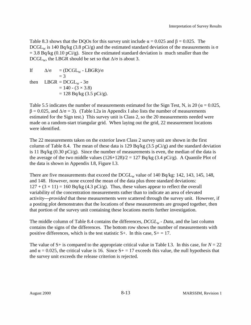
The 22 measurements taken on the exterior lawn Class 2 survey unit are shown in the firstcolumn of Table 8.4. The mean of these data is 129 Bq/kg (3.5 pCi/g) and the standard deviationis 11 Bq/kg (0.30 pCi/g). Since the number of measurements is even, the median of the data isthe average of the two middle values (126+128)/2 = 127 Bq/kg (3.4 pCi/g). A Quantile Plot ofthe data is shown in Appendix I.8, Figure I.3.

There are five measurements that exceed the DCGLW value of 140 Bq/kg: 142, 143, 145, 148,and 148. However, none exceed the mean of the data plus three standard deviations: 127 + (3 × 11) = 160 Bq/kg (4.3 pCi/g). Thus, these values appear to reflect the overallvariability of the concentration measurements rather than to indicate an area of elevatedactivity—provided that these measurements were scattered through the survey unit. However, ifa posting plot demonstrates that the locations of these measurements are grouped together, thenthat portion of the survey unit containing these locations merits further investigation.

The middle column of Table 8.4 contains the differences, DCGLW - Data, and the last columncontains the signs of the differences. The bottom row shows the number of measurements withpositive differences, which is the test statistic S+. In this case, S+ = 17.

The value of S+ is compared to the appropriate critical value in Table I.3. In this case, for N = 22and � = 0.025, the critical value is 16. Since S+ = 17 exceeds this value, the null hypothesis thatthe survey unit exceeds the release criterion is rejected.



Table 8.4 Example Sign Analysis: Class 2 Exterior Soil Survey Unit

Data (Bq/kg)

DCGLW-Data (Bq/kg) Sign

121 19 1

143 -3 -1

145 -5 -1

112 28 1

125 15 1

132 8 1

122 18 1

114 26 1

123 17 1

148 -8 -1

115 25 1

113 27 1

126 14 1

134 6 1

148 -8 -1

130 10 1

119 21 1

136 4 1

128 12 1

125 15 1

142 -2 -1

129 11 1

Number of positive differences S+ = 17

8.3.4 Sign Test Example: Class 3 Exterior Soil Survey Unit

For the Class 3 exterior soil survey unit, the one-sample nonparametric statistical test is again appropriate since the radionuclide of concern does not appear in background and radionuclidespecific measurements were made.

Table 8.3 shows that the DQOs for this survey unit include � = 0.025 and � = 0.01. The DCGLW

is 140 Bq/kg (3.8 pCi/g) and the estimated standard deviation of the measurements is � = 3.8 Bq/kg (0.10 pCi/g). Since the estimated standard deviation is much smaller than the DCGLW, the lower bound for the gray region should be set so that �/� is about 3.



If �/� = (DCGLW - LBGR)/� = 3

then LBGR = DCGLW - 3� = 140 - (3 × 4) = 128 Bq/kg (3.5 pCi/g).

Table 5.5 indicates that the sample size estimated for the Sign Test, N, is 23 (� = 0.025, � = 0.01, and �/� = 3). This survey unit is Class 3, so the measurements were made at random locations within the survey unit.

The 23 measurements taken on the exterior lawn are shown in the first column of Table 8.5. Notice that some of these measurements are negative (-0.37 in cell A6). This might occur if an analysis background (e.g., the Compton continuum under a spectrum peak) is subtracted to obtain the net concentration value. The data analysis is both easier and more accurate when numerical values are reported as obtained rather than reporting the results as “less than” or not detected. The mean of these data is 2.1 Bq/kg (0.057 pCi/g) and the standard deviation is 3.3 Bq/kg (0.089 pCi/g). None of the data exceed 2.1 + (3 × 3.3) = 12.0 Bq/kg (0.32 pCi/g). Since N is odd, the median is the middle (12th highest) value, namely 2.6 Bq/kg (0.070 pCi/g).

An initial review of the data reveals that every data point is below the DCGLW, so the survey unit meets the release criterion specified in Table 8.3. For purely illustrative purposes, the Sign test analysis is performed. The middle column of Table 8.5 contains the quantity DCGLW - Data. Since every data point is below the DCGLW, the sign of DCGLW - Data is always positive. The number of positive differences is equal to the number of measurements, N, and so the Sign test statistic S+ is 23. The null hypothesis will always be rejected at the maximum value of S+ (which in this case is 23) and the survey unit passes. Thus, the application of the Sign test in such cases requires no calculations and one need not consult a table for a critical value. If the survey is properly designed, the critical value must always be less than N.

Passing a survey unit without making a single calculation may seem an unconventional approach. However, the key is in the survey design which is intended to ensure enough measurements are made to satisfy the DQOs. As in the previous example, after the data are collected the conclusions and power of the test can be checked by constructing a retrospective power curve as outlined in Appendix I, Section I..9.

One final consideration remains regarding the survey unit classification: “Was any definite amount of residual radioactivity found in the survey unit?” This will depend on the MDC of the measurement method. Generally the MDC is at least 3 or 4 times the estimated measurement standard deviation. In the present case, the largest observation, 9.3 Bq/kg (0.25 pCi/g), is less than three times the estimated measurement standard deviation of 3.8 Bq/kg (0.10 pCi/g). Thus, it is unlikely that any of the measurements could be considered indicative of positive contamination. This means that the Class 3 survey unit classification was appropriate.


1

2

3

4

5

6

7

8

9

10

11

12

13

14

15

16

17

18

19

20

21

22

23

24

25


Table 8.5 Sign Test Example Data for Class 3 Exterior Survey Unit

A B C

Data DCGLW-Data Sign

3.0 137.0 1

3.0 137.0 1

1.9 138.1 1

0.37 139.6 1

-0.37 140.4 1

6.3 133.7 1

-3.7 143.7 1

2.6 137.4 1

3.0 137.0 1

-4.1 144.1 1

3.0 137.0 1

3.7 136.3 1

2.6 137.4 1

4.4 135.6 1

-3.3 143.3 1

2.1 137.9 1

6.3 133.7 1

4.4 135.6 1

-0.37 140.4 1

4.1 135.9 1

-1.1 141.1 1

1.1 138.9 1

9.3 130.7 1

Number of positive differences S+ = 23

If one determines that residual radioactivity is definitely present, this would indicate that the survey unit was initially mis-classified. Ordinarily, MARSSIM recommends a resurvey using a Class 1 or Class 2 design. If one determines that the survey unit is a Class 2, a resurvey might be avoided if the survey unit does not exceed the maximum size for such a classification. In this case, the only difference in survey design would be whether the measurements were obtained on a random or on a triangular grid. Provided that the initial survey’s scanning methodology is sufficiently sensitive to detect areas at DCGLW without the use of an area factor, this difference in the survey grids alone would not affect the outcome of the statistical analysis. Therefore, if the above conditions were met, a resurvey might not be necessary.



8.4 Contaminant Present in Background

The statistical tests discussed in this section will be used to compare each survey unit with an appropriately chosen, site-specific reference area. Each reference area should be selected on the basis of its similarity to the survey unit, as discussed in Section 4.5.

8.4.1 Two-Sample Statistical Test

The comparison of measurements from the reference area and survey unit is made using the Wilcoxon Rank Sum (WRS) test (also called the Mann-Whitney test). The WRS test should be conducted for each survey unit. In addition, the EMC is performed against each measurement to ensure that it does not exceed a specified investigation level. If any measurement in the remediated survey unit exceeds the specified investigation level, then additional investigation is recommended, at least locally, regardless of the outcome of the WRS test.

The WRS test is most effective when residual radioactivity is uniformly present throughout a survey unit. The test is designed to detect whether or not this activity exceeds the DCGLW. The advantage of the nonparametric WRS test is that it does not assume that the data are normally or log-normally distributed. The WRS test also allows for “less than” measurements to be present in the reference area and the survey units. As a general rule, the WRS test can be used with up to 40 percent “less than” measurements in either the reference area or the survey unit. However, the use of “less than” values in data reporting is not recommended as discussed in Section 2.3.5. When possible, report the actual result of a measurement together with its uncertainty.

The hypothesis tested by the WRS test is

Null HypothesisH0: The median concentration in the survey unit exceeds that in the reference area bymore than the DCGLW

versus

Alternative HypothesisHa: The median concentration in the survey unit exceeds that in the reference area by lessthan the DCGLW

The null hypothesis is assumed to be true unless the statistical test indicates that it should be rejected in favor of the alternative. One assumes that any difference between the reference area and survey unit concentration distributions is due to a shift in the survey unit concentrations to higher values (i.e., due to the presence of residual radioactivity in addition to background). Note that some or all of the survey unit measurements may be larger than some reference area



measurements, while still meeting the release criterion. Indeed, some survey unit measurements may exceed some reference area measurements by more than the DCGLW. The result of the hypothesis test determines whether or not the survey unit as a whole is deemed to meet the release criterion. The EMC is used to screen individual measurements.

Two assumptions underlying this test are: 1) samples from the reference area and survey unit are independent, identically distributed random samples, and 2) each measurement is independent of every other measurement, regardless of the set of samples from which it came.

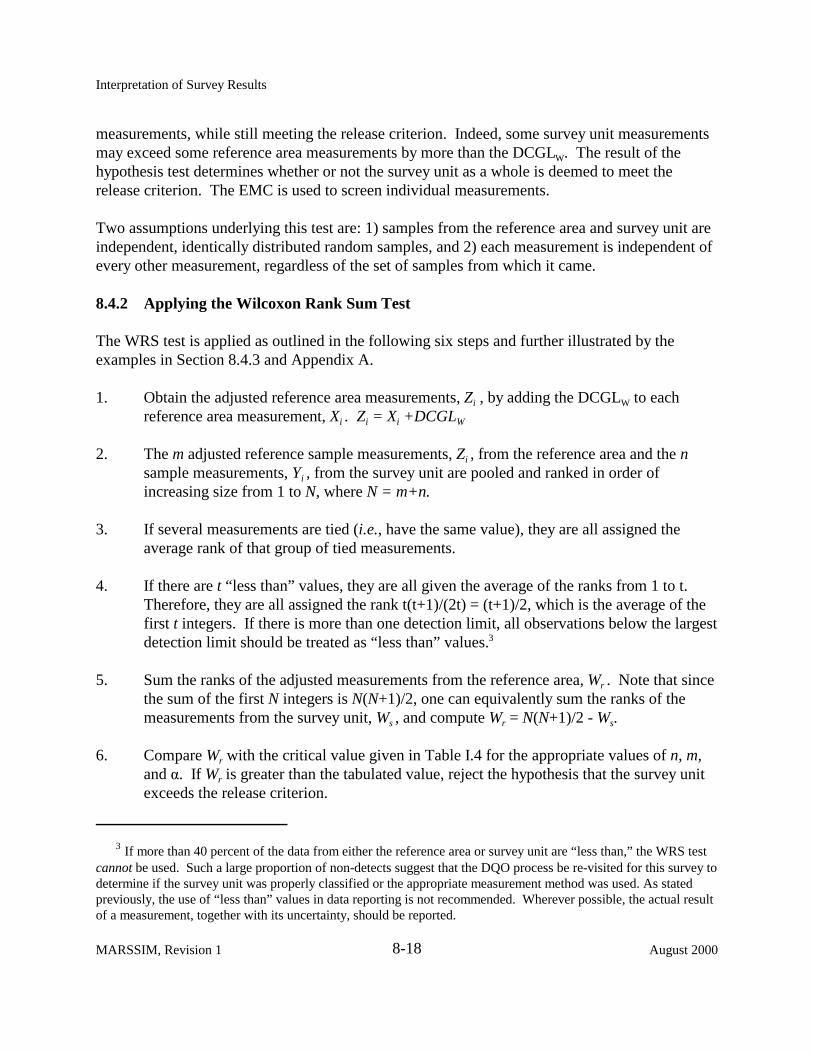
8.4.2 Applying the Wilcoxon Rank Sum Test

The WRS test is applied as outlined in the following six steps and further illustrated by the examples in Section 8.4.3 and Appendix A.

1. Obtain the adjusted reference area measurements, Zi , by adding the DCGLW to each reference area measurement, Xi . Zi = Xi +DCGLW

2. The m adjusted reference sample measurements, Zi , from the reference area and the n sample measurements, Yi , from the survey unit are pooled and ranked in order of increasing size from 1 to N, where N = m+n.

3. If several measurements are tied (i.e., have the same value), they are all assigned the average rank of that group of tied measurements.

4. If there are t “less than” values, they are all given the average of the ranks from 1 to t. Therefore, they are all assigned the rank t(t+1)/(2t) = (t+1)/2, which is the average of the first t integers. If there is more than one detection limit, all observations below the largest detection limit should be treated as “less than” values.3

5. Sum the ranks of the adjusted measurements from the reference area, Wr . Note that since the sum of the first N integers is N(N+1)/2, one can equivalently sum the ranks of the measurements from the survey unit, Ws , and compute Wr = N(N+1)/2 - Ws.

6. Compare Wr with the critical value given in Table I.4 for the appropriate values of n, m, and �. If Wr is greater than the tabulated value, reject the hypothesis that the survey unit exceeds the release criterion.

3 If more than 40 percent of the data from either the reference area or survey unit are “less than,” the WRS test cannot be used. Such a large proportion of non-detects suggest that the DQO process be re-visited for this survey to determine if the survey unit was properly classified or the appropriate measurement method was used. As stated previously, the use of “less than” values in data reporting is not recommended. Wherever possible, the actual result of a measurement, together with its uncertainty, should be reported.



8.4.3 Wilcoxon Rank Sum Test Example: Class 2 Interior Drywall Survey Unit

In this example, the gas-flow proportional counter measures total beta-gamma activity (see Appendix H) and the measurements are not radionuclide specific. The two-sample nonparametric test is appropriate for the Class 2 interior drywall survey unit because gross beta-gamma activity contributes to background even though the radionuclide of interest does not appear in background.

Table 8.3 shows that the DQOs for this survey unit include � = 0.025 and � = 0.05. The DCGLW

is 8,300 Bq/m2 (5,000 dpm per 100 cm2) and the estimated standard deviation of the measurements is about � = 1,040 Bq/m2 (625 dpm per 100 cm2). The estimated standard deviation is 8 times less than the DCGLW. With this level of precision, the width of the gray region can be made fairly narrow. As noted earlier, sample sizes do not decrease very much once �/� exceeds 3 or 4. In this example, the lower bound for the gray region was set so that �/� is about 4.

If �/� = (DCGLW - LBGR)/� = 4

then LBGR = DCGLW - 4� = 8,300 - (4 × 1,040) = 4,100 Bq/m2 (2,500 dpm per 100 cm2).

In Table 5.3, one finds that the number of measurements estimated for the WRS test is 11 in each survey unit and 11 in each reference area (� = 0.025, � = 0.05, and �/� = 4). (Table I.2b in Appendix I also lists the number of measurements estimated for the WRS test.) This survey unit was classified as Class 2, so the 11 measurements needed in the survey unit and the 11 measurements needed in the reference area were made using a random-start triangular grid.4

Table 8.6 lists the data obtained from the gas-flow proportional counter in units of counts per minute. A reading of 160 cpm with this instrument corresponds to the DCGLW of 8,300 Bq/m2

(5,000 dpm per 100 cm2). Column A lists the measurement results as they were obtained. The average and standard deviation of the reference area measurements are 44 and 4.4 cpm, respectively. The average and standard deviation of the survey unit measurements are 98 and 5.3 cpm, respectively.

4A random start systematic grid is used in Class 2 and 3 survey units primarily to limit the size of any potential elevated areas. Since areas of elevated activity are not an issue in the reference areas, the measurement locations can be either random or on a random start systematic grid (see Section 5.5.2.5).

June 2001 8-19 MARSSIM, Revision 1


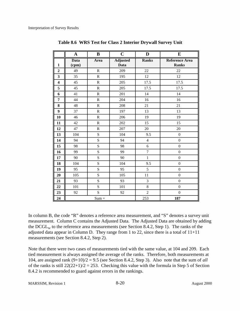
Table 8.6 WRS Test for Class 2 Interior Drywall Survey Unit

A B C D E

1 Data (cpm)

Ar ea Adjusted Data

Ranks Reference Area Ranks

2 49 R 209 22 22

3 35 R 195 12 12

4 45 R 205 17.5 17.5

5 45 R 205 17.5 17.5

6 41 R 201 14 14

7 44 R 204 16 16

8 48 R 208 21 21

9 37 R 197 13 13

10 46 R 206 19 19

11 42 R 202 15 15

12 47 R 207 20 20

13 104 S 104 9.5 0

14 94 S 94 4 0

15 98 S 98 6 0

16 99 S 99 7 0

17 90 S 90 1 0

18 104 S 104 9.5 0

19 95 S 95 5 0

20 105 S 105 11 0

21 93 S 93 3 0

22 101 S 101 8 0

23 92 S 92 2 0

24 Sum = 253 187

In column B, the code “R” denotes a reference area measurement, and “S” denotes a survey unit measurement. Column C contains the Adjusted Data. The Adjusted Data are obtained by adding the DCGLW to the reference area measurements (see Section 8.4.2, Step 1). The ranks of the adjusted data appear in Column D. They range from 1 to 22, since there is a total of 11+11 measurements (see Section 8.4.2, Step 2).

Note that there were two cases of measurements tied with the same value, at 104 and 209. Each tied measurement is always assigned the average of the ranks. Therefore, both measurements at 104, are assigned rank (9+10)/2 = 9.5 (see Section 8.4.2, Step 3). Also note that the sum of all of the ranks is still 22(22+1)/2 = 253. Checking this value with the formula in Step 5 of Section 8.4.2 is recommended to guard against errors in the rankings.



Column E contains only the ranks belonging to the reference area measurements. The total is 187. This is compared with the entry for the critical value of 156 in Table I.4 for � = 0.025, with n = 11 and m =11. Since the sum of the reference area ranks is greater than the critical value, the null hypothesis (i.e., that the average survey unit concentration exceeds the DCGLW) is rejected.

The analysis for the WRS test is very well suited to the use of a computer spreadsheet. The spreadsheet formulas used for the example above are given in Appendix I.10, Table I.11.

8.4.4 Class 1 Interior Concrete Survey Unit

As in the previous example, the gas-flow proportional counter measures total beta-gamma activity (see Appendix H) and the measurements are not radionuclide specific. The two-sample nonparametric test is appropriate for the Class 1 interior concrete survey unit because gross beta-gamma activity contributes to background even though the radionuclide of interest does not appear in background.

Appendix A provides a detailed description of the calculations for the Class 1 interior concrete survey unit.

8.4.5 Multiple Radionuclides

The use of the unity rule when there is more than one radionuclide to be considered is discussed in Appendix I.11. An example application appears in Section I.11.4.

8.5 Evaluating the Results: The Decision

Once the data and the results of the tests are obtained, the specific steps required to achieve site release depend on the procedures instituted by the governing regulatory agency and site-specific ALARA considerations. The following suggested considerations are for the interpretation of the test results with respect to the release limit established for the site or survey unit. Note that the tests need not be performed in any particular order.

8.5.1 Elevated Measurement Comparison

The Elevated Measurement Comparison (EMC) consists of comparing each measurement from the survey unit with the investigation levels discussed in Section 5.5.2.6 and Section 8.2.5. The EMC is performed for both measurements obtained on the systematic-sampling grid and for locations flagged by scanning measurements. Any measurement from the survey unit that is equal to or greater than an investigation level indicates an area of relatively high concentrations that should be investigated—regardless of the outcome of the nonparametric statistical tests.



The statistical tests may not reject H0 when only a very few high measurements are obtained in the survey unit. The use of the EMC against the investigation levels may be viewed as assurance that unusually large measurements will receive proper attention regardless of the outcome of those tests and that any area having the potential for significant dose contributions will be identified. The EMC is intended to flag potential failures in the remediation process. This should not be considered the primary means to identify whether or not a site meets the release criterion.

The derived concentration guideline level for the EMC is:

DCGLEMC ' Am × DCGLW 8-1

where Am is the area factor for the area of the systematic grid area. Note that DCGLEMC is an a priori limit, established both by the DCGLW and by the survey design (i.e., grid spacing and scanning MDC). The true extent of an area of elevated activity can only be determined after performing the survey and taking additional measurements. Upon the completion of further investigation, the a posteriori limit, DCGLEMC = Am × DCGLW , can be established using the value of Am appropriate for the actual area of elevated concentration. The area of elevated activity is generally bordered by concentration measurements below the DCGLW. An individual elevated measurement on a systematic grid could conceivably represent an area four times as large as the systematic grid area used to define the DCGLEMC. This is the area bounded by the nearest neighbors of the elevated measurement location. The results of the investigation should show that the appropriate DCGLEMC is not exceeded. Area factors are discussed in Section 5.5.2.4.

If measurements above the stated scanning MDC are found by sampling or by direct measurement at locations that were not flagged by the scanning survey, this may indicate that the scanning method did not meet the DQOs.

The preceding discussion primarily concerns Class 1 survey units. Measurements exceeding DCGLW in Class 2 or Class 3 areas may indicate survey unit mis-classification. Scanning coverage for Class 2 and Class 3 survey units is less stringent than for Class 1. If the investigation levels of Section 8.2.5 are exceeded, an investigation should: 1) ensure that the area of elevated activity discovered meets the release criterion, and 2) provide reasonable assurance that other undiscovered areas of elevated activity do not exist. If further investigation determines that the survey unit was mis-classified with regard to contamination potential, then a resurvey using the method appropriate for the new survey unit classification may be appropriate.



8.5.2 Interpretation of Statistical Test Results

The result of the statistical test is the decision to reject or not to reject the null hypothesis. Provided that the results of investigations triggered by the EMC were resolved, a rejection of the null hypothesis leads to the decision that the survey unit meets the release criterion. However, estimating the average residual radioactivity in the survey unit may also be necessary so that dose or risk calculations can be made. This estimate is designated �. The average concentration is generally the best estimator for � (EPA 1992g). However, only the unbiased measurements from the statistically designed survey should be used in the calculation of �.

If residual radioactivity is found in an isolated area of elevated activity—in addition to residual radioactivity distributed relatively uniformly across the survey unit—the unity rule (Section 4.3.3) can be used to ensure that the total dose is within the release criterion:

� %

(average concentration i n elevated area & �)< 1

DCGLW (area factor for elevated area)(DCGLW)

If there is more than one elevated area, a separate term should be included for each. When calculating � for use in this inequality, measurements falling within the elevated area may be excluded providing the overall average in the survey unit is less than the DCGLW. As an alternative to the unity rule, the dose or risk due to the actual residual radioactivity distribution can be calculated if there is an appropriate exposure pathway model available. Note that these considerations generally apply only to Class 1 survey units, since areas of elevated activity should not exist in Class 2 or Class 3 survey units.

A retrospective power analysis for the test will often be useful, especially when the null hypothesis is not rejected (see Appendix I.9). When the null hypothesis is not rejected, it may be because it is in fact true, or it may be because the test did not have sufficient power to detect that it is not true. The power of the test will be primarily affected by changes in the actual number of measurements obtained and their standard deviation. An effective survey design will slightly overestimate both the number of measurements and the standard deviation to ensure adequate power. This insures that a survey unit is not subjected to additional remediation simply because the final status survey is not sensitive enough to detect that residual radioactivity is below the guideline level. When the null hypothesis is rejected, the power of the test becomes a somewhat moot question. Nonetheless, even in this case, a retrospective power curve can be a useful diagnostic tool and an aid to designing future surveys.

8.5.3 If the Survey Unit Fails

The guidance provided in MARSSIM is fairly explicit concerning the steps that should be taken to show that a survey unit meets release criteria. Less has been said about the procedures that should be used if at any point the survey unit fails. This is primarily because there are many different ways that a survey unit may fail the final status survey. The overall level of residual

June 2001 8-23 MARSSIM, Revision 1

8-2


radioactivity may not pass the nonparametric statistical tests. Further investigation following the elevated measurement comparison may show that there is a large enough area with a concentration too high to meet the release criterion. Investigation levels may have caused locations to be flagged during scanning that indicate unexpected levels of residual radioactivity for the survey unit classification. Site-specific information is needed to fully evaluate all of the possible reasons for failure, their causes, and their remedies.

When a survey unit fails to demonstrate compliance with the release criterion, the first step is to review and confirm the data that led to the decision. Once this is done, the DQO Process (Appendix D) can be used to identify and evaluate potential solutions to the problem. The level of residual radioactivity in the survey unit should be determined to help define the problem. Once the problem has been stated the decision concerning the survey unit should be developed into a decision rule. Next, determine the additional data, if any, needed to document that the survey unit demonstrates compliance with the release criterion. Alternatives to resolving the decision statement should be developed for each survey unit that fails the tests. These alternatives are evaluated against the DQOs, and a survey design that meets the objectives of the project is selected.

For example, a Class 2 survey unit passes the nonparametric statistical tests, but has several measurements on the sampling grid that exceed the DCGLW. This is unexpected in a Class 2 area, and so these measurements are flagged for further investigation. Additional sampling confirms that there are several areas where the concentration exceeds the DCGLW. This indicates that the survey unit was mis-classified. However, the scanning technique that was used was sufficient to detect residual radioactivity at the DCGLEMC calculated for the sample grid. No areas exceeding the DCGLEMC where found. Thus, the only difference between the final status survey actually done, and that which would be required for a Class 1 area, is that the scanning may not have covered 100% of the survey unit area. In this case, one might simply increase the scan coverage to 100%. Reasons why the survey unit was misclassified should be noted. If no areas exceeding the DCGLEMC are found, the survey unit essentially demonstrates compliance with the release criterion as a Class 1 survey unit.

If, in the example above, the scanning technique was not sufficiently sensitive, it may be possible to re-classify as Class 1 only that portion of the survey unit containing the higher measurements. This portion would be re-sampled at the higher measurement density required for a Class 1 survey unit, with the rest of the survey unit remaining Class 2.

A second example might be a Class 1 Survey unit that passes the nonparametric statistical tests and contains some areas that were flagged for investigation during scanning. Further investigation, sampling and analysis indicates one area is truly elevated. This area has a concentration that exceeds the DCGLW by a factor greater than the area factor calculated for its actual size. This area is then remediated. Remediation control sampling shows that the residual



radioactivity was removed, and no other areas were contaminated with removed material. In this case one may simply document the original final status survey, the fact that remediation was performed, the results of the remedial action support survey, and the additional remediation data. In some cases, additional final status survey data may not be needed to demonstrate compliance with the release criterion.

As a last example, consider a Class 1 area which fails the nonparametric statistical tests. Confirmatory data indicates that the average concentration in the survey unit does exceed the DCGLW over a majority of its area. This indicates remediation of the entire survey unit is necessary, followed by another final status survey. Reasons for performing a final status survey in a survey unit with significant levels of residual radioactivity should be noted.

These examples are meant to illustrate the actions that may be necessary to secure the release of a survey unit that has failed to meet the release criterion. The DQO Process should be revisited to plan how to attain the original objective, that is to safely release the survey unit by showing that it meets the release criterion. Whatever data are necessary to meet this objective will be in addition to the final status survey data already in hand.

8.5.4 Removable Activity

Some regulatory agencies may require that smear samples be taken at indoor grid locations as an indication of removable surface activity. The percentage of removable activity assumed in the exposure pathway models has a great impact on dose calculations. However, measurements of smears are very difficult to interpret quantitatively. Therefore, the results of smear samples should not be used for determining compliance. Rather, they should be used as a diagnostic tool to determine if further investigation is necessary.

8.6 Documentation

Documentation of the final status survey should provide a complete and unambiguous record of the radiological status of the survey unit relative to the established DCGLs. In addition, sufficient data and information should be provided to enable an independent evaluation of the results of the survey including repeating measurements at some future time. The documentation should comply with all applicable regulatory requirements. Additional information on documentation is provided in Chapter 3, Chapter 5, Chapter 9, and Appendix N.

Much of the information in the final status report will be available from other decommissioning documents. However, to the extent practicable, this report should be a stand-alone document with minimum information incorporated by reference. This document should describe the



instrumentation or analytical methods used, how the data were converted to DCGL units, the process of comparing the results to the DCGLs, and the process of determining that the data quality objectives were met.

The results of actions taken as a consequence of individual measurements or sample concentrations in excess of the investigation levels should be reported together with any additional data, remediation, or re-surveys performed to demonstrate that issues concerning potential areas of elevated activity were resolved. The results of the data evaluation using statistical methods to determine if release criteria were satisfied should be described. If criteria were not met or if results indicate a need for additional data, appropriate further actions should be determined by the site management in consultation with the responsible regulatory agency.



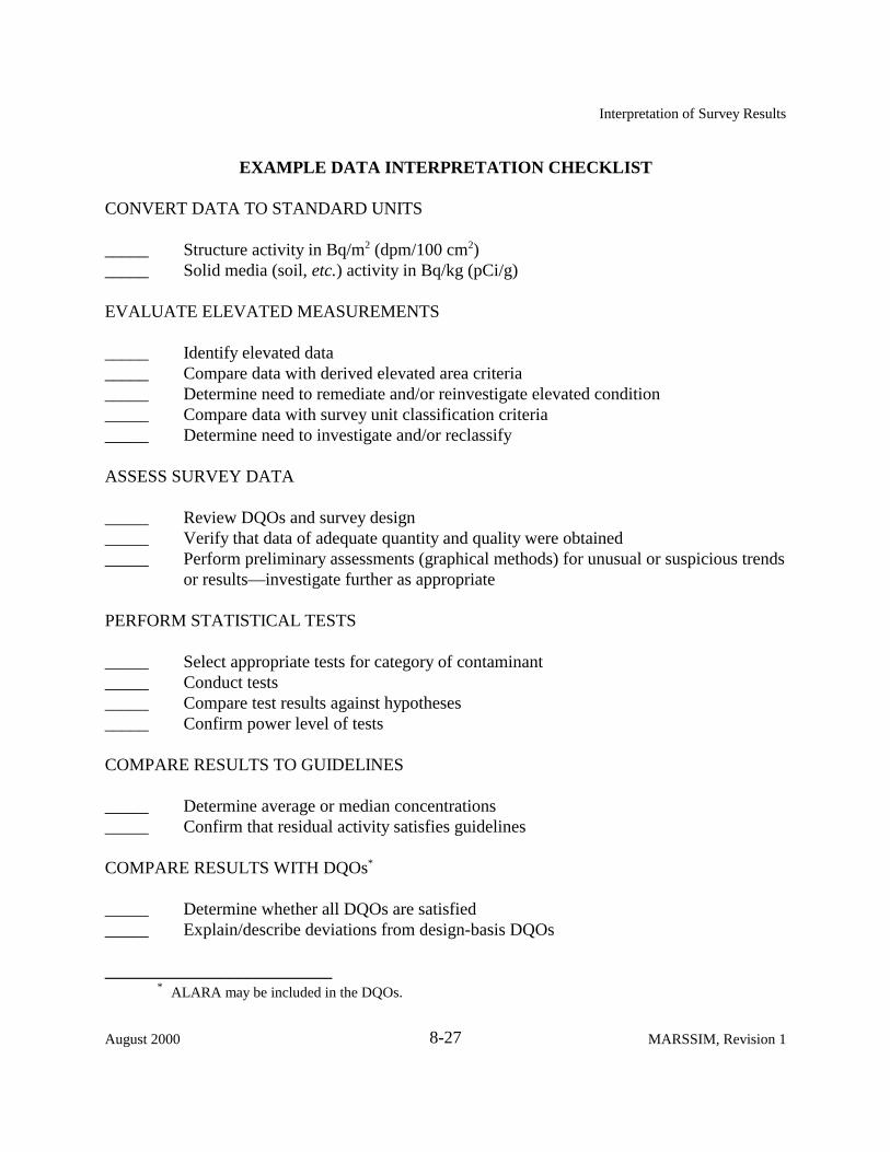
EXAM PLE DATA INTERP RETATION CHECK LIST

CONVERT DATA TO STANDARD UNITS

_____ Structure activity in Bq/m2 (dpm/100 cm2) _____ Solid media (soil, etc.) activity in Bq/kg (pCi/g)

EVALUATE ELEVATED MEASUREMENTS

_____ Identify elevated data_____ Compare data with derived elevated area criteria_____ Determine need to remediate and/or reinvestigate elevated condition_____ Compare data with survey unit classification criteria_____ Determine need to investigate and/or reclassify

ASSESS SURVEY DATA

_____ Review DQOs and survey design_____ Verify that data of adequate quantity and quality were obtained_____ Perform preliminary assessments (graphical methods) for unusual or suspicious trends

or results—investigate further as appropriate

PERFORM STATISTICAL TESTS

_____ Select appropriate tests for category of contaminant_____ Conduct tests_____ Compare test results against hypotheses_____ Confirm power level of tests

COMPARE RESULTS TO GUIDELINES

_____ Determine average or median concentrations_____ Confirm that residual activity satisfies guidelines

COMPARE RESULTS WITH DQOs*

_____ Determine whether all DQOs are satisfied _____ Explain/describe deviations from design-basis DQOs

__________________________ * ALARA may be included in the DQOs.


8 interpretation of survey results 8.1 … · 8 interpretation of survey results ... adequate, but...

Documents