8 excel pivot table examples – how to make a pivottable! · pdf file8 excel pivot table...

8 Excel Pivot Table Examples – How to Make a PivotTable!

1

The PivotTable feature is perhaps the most important component in Excel. PivotTable is making one or more new table from a given data table.

This article is part of my series: Excel Pivot Table Tutorials for Dummies [Step by Step].

The best way to understand pivot table is to see one. Start with the following Figure. This figure shows a portion of the data we have used creating the pivot tables in this chapter.

We shall create the Pivot Tables from this data table in this chapter.

Our example shows that data is in a table, but you can make pivot tables from any kind of data.

Download Working Files

To follow me with this tutorial, at first download the working file(s) that I have used to create this tutorial. Click the green button below; download the working file. I have created total 8 Pivot Tables. You will get the pivot tables in the PT1, PT2, PT3, PT4, PT5, PT6, PT7 and PT8 worksheets.

https://www.exceldemy.com/step-by-step-excel-pivot-table-tutorials-for-dummies/

https://www.exceldemy.com/wp-content/uploads/2014/01/Bank-accounts5.xlsx


2

The above table consists of new account information of a bank. The bank has three branches: Central, North Country, and Westside. The table has 712 rows. Each row represents a new account opened at the bank. The table has the following columns:

• The date the bank account was opened • The day of the week the bank account was opened • The opening amount • The bank account type (CD, checking, savings, or IRA) • Who opened the bank account (whether a teller or a new account representative) • The branch at which the bank account was opened (Central, Westside, or North

County) • The type of customer (whether an existing customer or a new customer)

Creating a pivot table manually

In our sample file Bank-accounts.xlsx, our database worksheet is named "data". This database contains a good amount of information. But in its current form, the data doesn't reveal much to you.

These following questions, the bank's management may want to know:

• What is the total amount of new deposits, broken down by account type and branch?

• What is the daily total new deposit amount for each branch? • Which day of the week generates the most deposits? • How many new bank accounts were opened at each branch, broken down by

account type? • What’s the dollar distribution of the different account types? • What types of bank accounts do tellers open most often? • How does the Central branch compare with the other two branches? • In which branch do tellers open the most savings accounts for new customers?

You can sort the data and create formulas to answer these questions. But using pivot table is a better choice, pivot table takes few seconds, doesn't require formula and produces a professional-looking report.

In addition, analyzing data with pivot tables makes less error than with creating formulas.


3

Pivot Table Examples

1) What is the total amount of new deposits, broken down by account type and branch?

Now we shall create a pivot table using the sample file to answer this question. Follow this process:

Step 1: Specifying the data range

If your data is in a worksheet range, just select any cell in the range. We select cell A2 in

our "data" worksheet. Now choose Insert ➪ Tables ➪ PivotTable. The Create PivotTable dialog box will appear. Excel automatically guess your data range. For this example, we are going to create our pivot table in a new worksheet. See the following screenshot:

In the Create PivotTable dialog box, you tell Excel where the data is and where you want the place the pivot table.

Step 2: Creating blank pivot table

Click OK to choose the options as it is. Excel creates an empty pivot table and displays a PivotTable Fields task pane. Look at the following figure:


4

We shall use this PivotTable Fields task pane to build our pivot table.

Step 3: Laying out the pivot table

Now we shall work on the PivotTable Fields task pane. PivotTable Fields task pane has two parts: the upper part, where the field names reside, and the lower part, where you will place the upper part's field names as per your necessity. In our example, upper part of PivotTable Fields task pane holds Date, Weekday, Amount, AcctType, OpenedBy, Branch, Customer fields. The lower part has Filters, Columns, Rows, and Values area.

The following steps will create the pivot table:

1. Drag the Amount field into the Values area. The pivot table will display the total of all the values in the Amount column.

2. Drag the AcctType field into the Rows area. The pivot table will show now the total amount for each of the account types.

3. Now, drag the Branch field into the Columns area.The pivot table will show now the amount for each account type, cross-tabulated by branch. Observe closely. You will find that total amount of each AccType is calculated on the right side of the pivot table. At the same time, total amount opened in every branch is also calculated at the bottom of the pivot table.


5

Dragging the fields to the lower part of PivotTable.

The following figure gives us our desired Pivot Table. From this Pivot Table, we can find out easily grand total of amount opened in Westside branch. The pivot table is in "PT1" sheet. We have changed the sheet name to "PT1" after the creation of pivot table.


6

The pivot table is showing the summary of our data.

2) What is the daily total new deposit amount for each branch?

This time we shall place Amount field in VALUES area, Branch field in COLUMNS area, and Date field in ROWS area. The pivot table is in "PT2" sheet. We have changed the sheet name to "PT2" after the creation of pivot table.

Here is a screenshot.

Pivot Table 2.

3) Which day of the week generates the most deposits?

To get this pivot table, we shall place the Weekday field in ROWS area and Amount field in VALUES area.

We want to use conditional formatting to the data range B4: B9 to make you understand easily which day is making more deposits. To do this select cell range B4: B9 and choose

Home ➪ Style ➪ Conditional Formatting ➪ Data Bars ➪ Gradient Fill ➪ Green Data Bar.

The pivot table is in "PT3" sheet. We have changed the sheet name to "PT3" after the creation of pivot table.


7

Using conditional formatting, we have made this pivot table more understandable.

4) How many new bank accounts were opened at each branch, broken down by account type?

To get this pivot table, we shall place Amount field in VALUES area, AcctType field in COLUMNS area, and Branch field in ROWS area.

You will get a pivot table, but this one shows the total amount of deposits, broken down by account types and branch like our first created pivot table. We have to change some options to get our required one.

Right click on any value of the pivot table and then use the following figure to change the option.


8

Right click on any value in the pivot table and select Summarize Values By ⇒ Count

After selecting the Count option, our pivot table will look like this.

Pivot Table with count values.



9

5) What’s the dollar distribution of the different account types?

Dollar distribution means, say you may want to know how many accounts were opened in the range of 1-5000. In our example, total 712 accounts were opened, among them, 253 accounts were opened in the range of 1-5000 range. In percentage, we can say about 35.53% accounts were opened in 1-5000 dollar range.

We shall create a pivot table showing all the dollar distributions.

Step 1: Grouping the amount values

At first place the Amount field in the rows section at the bottom of the PivotTable Fields task pane. This will create a figure like this. Right click on any value in the pivot table, a shortcut menu will appear.


10

When Amount data is placed in Rows section, data is placed ungrouped. To make data in the group, click the Group option as per this image.

Select Group from the options, Grouping dialog box will appear. Enter 1, 100000, and 5000 in three fields respectively.

Grouping data with the help of Grouping dialog box.

Click OK, your pivot table will look like this.


11

Data are grouped in ranges.

Step 2: Counting accounts

Place the Amount field again in the Values section. The pivot table will look like this.

Pivot table summarized as Sum.


12

We have to summarize our pivot table by Count. To do this, right-click on any values, a shortcut menu will appear and choose Summarize Values By⇒ Count. Your pivot table will look like this.

Data summarized by count

Step 3: Dollar distribution in %

Repeat what we have done in step 2. Another same column will be added. Click any cell in the last column and choose Shows Values as ⇒ % of Grand Total. The table will look like this.


13

Pivot Table is showing in the percentage of Grand Total.

Change the headers name to Amount, Count, and % of Grand Total respectively. This is your final pivot table.

Final Pivot Table


6) What types of bank accounts do tellers open most often?

To find out what types of bank accounts tellers open most is simple.

Step 1

Place OpenedBy field in the FILTERS area PivotTable Fields at first.

Step 2

Now place the AcctType field in the ROWS area in the PivotTable Fields task pane.

Step 3

Now place the Amount field in the VALUES area in the PivotTable Fields task pane.


14

Step 4

Repeat step 3.

Step 5

Right click on any value in the last column and choose Shows Values as ⇒ % of Grand Total from the shortcut menu.

Step 6

Change the header name of the last two columns to Accounts and PCT respectively.

Step 7

Select cell range C4: C7 and apply this conditional formatting: Home ➪ Style ➪

Conditional Formatting ➪ Data Bars ➪ Gradient Fill ➪ Green Data Bar. Click OpenedBy drop down list and choose Teller.

Final Pivot Table we get


7) How does the Central branch compare with the other two branches?

To achieve this pivot table, we shall learn how to combine two columns into a pivot table.

• Drag the AcctType field is in the Rows section. • Drag the Branch field is in the Columns section. • The Amount field is in the Values section.


15

You will get a pivot table like this.

Pivot Table when dragged the above fields in the bottom part of the PivotTable Fields task

pane

Now select both North County and Westside columns and right click and choose Group from the shortcut menu. This will combine these two branches into a new category (Group 1). Grouping also creates a new field in the PivotTable Fields task pane. In our case, the new field is named Branch2 in the PivotTable Fields. You can change the label in the pivot table to Other Branches.

After grouping the North County and Westside branches, you can now easily compare between the Central branch and the other two branches. See the following figure.

Pivot table when grouped two branches and transformed into one.

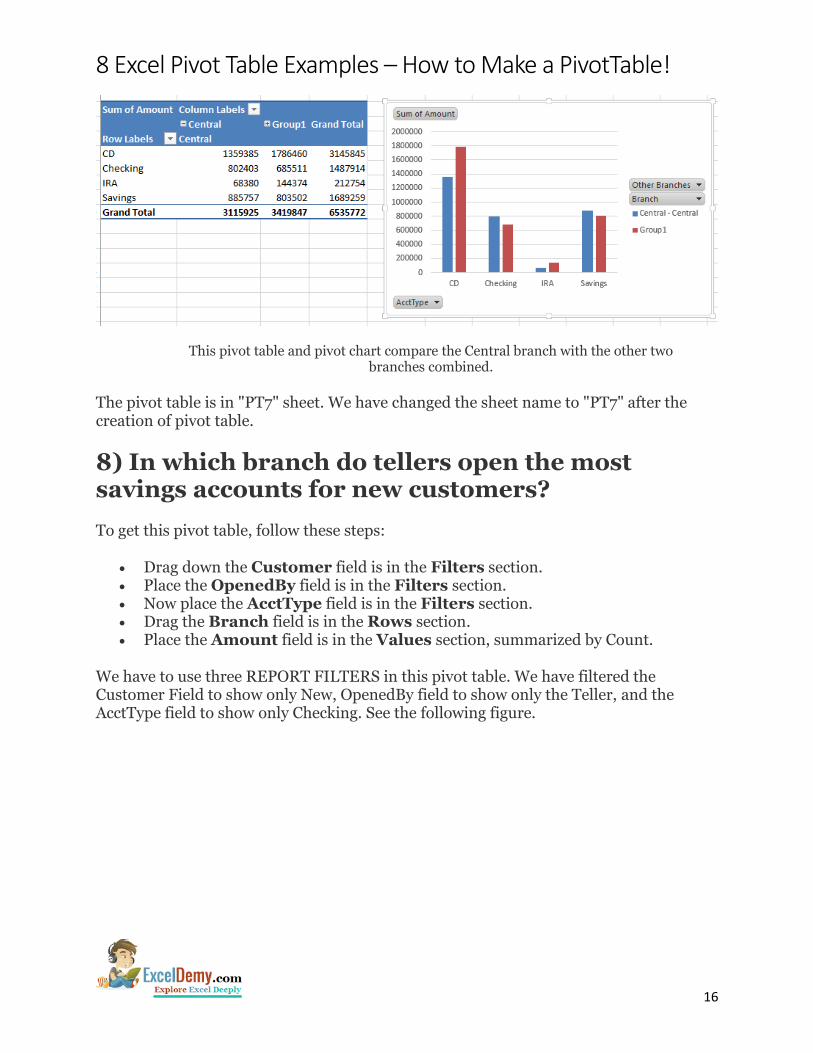
We want to add a chart for easy comparison. Choose PIVOTTABLE TOOLS ⇒ ANALYZE ⇒Tools ⇒ PivotChart ⇒ Clustered Column chart. We have got our desired Pivot Table. Look at this.


16

This pivot table and pivot chart compare the Central branch with the other two branches combined.


8) In which branch do tellers open the most savings accounts for new customers?

To get this pivot table, follow these steps:

• Drag down the Customer field is in the Filters section. • Place the OpenedBy field is in the Filters section. • Now place the AcctType field is in the Filters section. • Drag the Branch field is in the Rows section. • Place the Amount field is in the Values section, summarized by Count.

We have to use three REPORT FILTERS in this pivot table. We have filtered the Customer Field to show only New, OpenedBy field to show only the Teller, and the AcctType field to show only Checking. See the following figure.


17

This pivot table uses three Filters.


Happy Excelling :)

8 excel pivot table examples – how to make a pivottable! · pdf file8 excel pivot table...

Documents