8:; ' # '7& *#8 & 9cdn.intechopen.com/pdfs-wm/20923.pdf · integrating river bed...

3,350+OPEN ACCESS BOOKS

108,000+INTERNATIONAL

AUTHORS AND EDITORS115+ MILLION

DOWNLOADS

BOOKSDELIVERED TO

151 COUNTRIES

AUTHORS AMONG

TOP 1%MOST CITED SCIENTIST

12.2%AUTHORS AND EDITORS

FROM TOP 500 UNIVERSITIES

Selection of our books indexed in theBook Citation Index in Web of Science™

Core Collection (BKCI)

Chapter from the book Sediment Transport in Aquatic EnvironmentsDownloaded from: http://www.intechopen.com/books/sediment-transport-in-aquatic-environments

PUBLISHED BY

World's largest Science,Technology & Medicine

Open Access book publisher

Interested in publishing with IntechOpen?Contact us at [email protected]

http://www.intechopen.com/books/sediment-transport-in-aquatic-environments

mailto:[email protected]

15

Integrating River Bed Dynamics to Flood Risk Assessment

Clemens Neuhold, Philipp Stanzel and Hans Peter Nachtnebel

University of Natural Resources and Life SciencesVienna Austria

1. Introduction

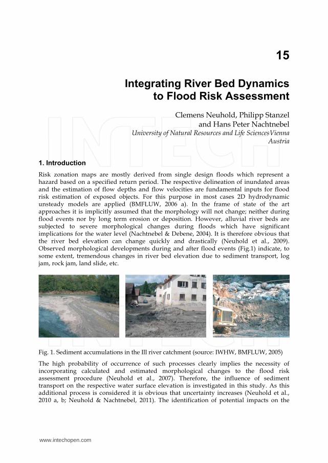
Risk zonation maps are mostly derived from single design floods which represent a hazard based on a specified return period. The respective delineation of inundated areas and the estimation of flow depths and flow velocities are fundamental inputs for flood risk estimation of exposed objects. For this purpose in most cases 2D hydrodynamic unsteady models are applied (BMFLUW, 2006 a). In the frame of state of the art approaches it is implicitly assumed that the morphology will not change; neither during flood events nor by long term erosion or deposition. However, alluvial river beds are subjected to severe morphological changes during floods which have significant implications for the water level (Nachtnebel & Debene, 2004). It is therefore obvious that the river bed elevation can change quickly and drastically (Neuhold et al., 2009). Observed morphological developments during and after flood events (Fig.1) indicate, to some extent, tremendous changes in river bed elevation due to sediment transport, log jam, rock jam, land slide, etc.

Fig. 1. Sediment accumulations in the Ill river catchment (source: IWHW, BMFLUW, 2005)

The high probability of occurrence of such processes clearly implies the necessity of incorporating calculated and estimated morphological changes to the flood risk assessment procedure (Neuhold et al., 2007). Therefore, the influence of sediment transport on the respective water surface elevation is investigated in this study. As this additional process is considered it is obvious that uncertainty increases (Neuhold et al., 2010 a, b; Neuhold & Nachtnebel, 2011). The identification of potential impacts on the

www.intechopen.com

Sediment Transport in Aquatic Environments 318

water surface elevation and accordingly the possible inundation depth as well as delineation could, however, lead to an increase of awareness and adaptation of flood risk management strategies. The study focuses on implications related to hazard assessment covering aspects of hydrology, hydraulics and sediment transport. Further, the study aims at enhancing approaches of vulnerability assessment and therefore, damage estimation by providing a direct link of probability distribution functions of inundation depths with the respective damage functions of flood-prone utilisations (damage-probability relationship). The concept is tested in the river Ill catchment in the Western Austrian Alps which has suffered major floods during the recent past (1999, 2000 and 2005). The River Ill, with a mean annual discharge of 66 m³/s and a catchment area of approximately 1300m² is the main river catchment in south-eastern Vorarlberg, the most-western federal state of Austria (Fig.2). The catchment area is characterized by torrential tributaries, hydraulic structures, hydropower plants and complex morphological characteristics. Hydro-meteorological observations of precipitation, air temperature and runoff were gathered. Elevations range from 400 to 3000 m. a. s. l. and the mean annual precipitation averages 1700 mm. A 100-year flood event is estimated at 820 m³/s. Current, as well as historical surveying data (since 1978), were provided for 60 km of the River Ill and, altogether, 15 km of 8 tributaries comprising cross section measurements (with distances of 100 m on average) and airborne laser scan data. Sediment samples were drawn in 71 locations. Additional information on geographical features of the catchment (elevation, land cover, cadastral information and soil type) and on hydropower influence on the runoff regime is considered.

Fig. 2. Study area: Austria and the Ill river catchment in the west

2. Methodology

The applied methodological approach is elaborated to analyse and quantify the variability and uncertainty of single steps of hazard assessment and to enhance vulnerability assessment. Therefore, the estimation of hydrological input, possible changes in river bed

www.intechopen.com

Integrating River Bed Dynamics to Flood Risk Assessment 319

elevation due to sediment transport and the effects on water surface elevations are dissected. Vulnerability analyses and damage estimation tools are methodologically improved by connecting the overtopping probability, the variability of inundation depth and object related damage functions to obtain a damage-probability relationship (Fig.3). Initially, the hydrology of the catchment is simulated with a semi-distributed precipitation-runoff model. Variability of the hydrograph is obtained by generating numerous scenarios with different initial moisture conditions and by considering different spatial and temporal distributions, durations and amounts of rainfall. The hydrologic model provides runoff scenarios which are subsequently used as an input for the hydraulic and sediment transport model. Additionally, the variability of possible morphological changes due to torrential sediment entry is analysed. For this purpose scenarios with randomly drawn sediment loads from torrential inflows based on probability distribution functions are developed to account for the high variability and unpredictability of torrential sediment input to the system. The calculated morphological changes of the river bed provide a basis to estimate the variability of water surface levels and inundation lines which need to be considered in flood hazard maps and flood risk maps. For each scenario the water table, river bed elevation and the respective inundation lines as well as inundation depths are calculated. Therefore, every single exposed object is linked to a distribution function consisting of estimated damages related to flood inundation depth and inundation probability.

Fig. 3. Scheme of approach to derive the damage probability of vulnerable utilisations

2.1 Hydrologic input generation

The continuous, semi-distributed rainfall-runoff model, COSERO, developed by the Institute of Water Management, Hydrology and Hydraulic Engineering, BOKU (Nachtnebel et al., 1993, Kling, 2002 among others) is applied to the entire Ill catchment. The model accounts for processes of snow accumulation and melt, interception, evapotranspiration, infiltration, soil storage, runoff generation and routing. Separation of runoff into fast surface runoff, inter flow and base flow is calculated by means of a cascade of linear and non-linear

www.intechopen.com


reservoirs. Spatial discretisation relies on the division of the watersheds into sub-basins and subsequently into hydrologic response units (HRUs). The Ill watershed is divided into 37 sub-basins, based on the location of runoff gauges, anthropogenic diversions and reservoirs, with sub-basin areas ranging from 10 to 200 km² (Fig.2). 828 HRUs, with a mean area of 1.6 km², are derived by intersection of 200 m-elevation bands with soil type data (Peticzka and Kriz, 2005) and land use data (Fürst and Hafner, 2005). The model is calibrated and validated based on observed discharge hydrographs of 6 years with continuous daily records and hourly records for 16 flood periods, measured at 14 gauges (Stanzel et al., 2007). Calibrated parameters of gauged sub-basins are transferred to neighbouring ungauged sub-basins. Storage coefficients for base flow and interflow, which correlated well with catchment size for the calibrated sub-basins, are assigned according to this relation. After this, storage coefficients for fast runoff are allocated in order to achieve characteristics of runoff separation into surface flow, interflow and base flow as simulated in neighbouring calibrated sub-basins with similar physical features. Nash-Sutcliffe model efficiencies (Nash and Sutcliffe, 1970) between 0.80 and 0.90 for the calibration period and between 0.75 and 0.85 for the validation period are achieved. Mean relative peak errors of the 16 simulated flood periods range between -15 % and +10 %. After calibration, the rainfall-runoff model is applied to simulate flood runoff scenarios. Design storms with assumed return periods of 100 years are used as input. The underlying assumption of using design storms with a 100-year recurrence interval is that they may produce flood peaks of the same return period. While this premise can be regarded as appropriate for design purposes, it is clear that a rainstorm with a given return period may cause a flood with a higher or lower return period (Larson and Reich, 1972). This is due to factors affecting the runoff event like the distribution of rainfall in time and space or antecedent soil moisture and river discharge. Therefore, several scenarios, with variations of major influencing factors, are defined. Precipitation scenarios are obtained by varying total precipitation depth, storm duration and temporal and spatial distributions. Each rainfall scenario is combined with three different initial catchment conditions, which are selected from simulated state variables of historical flood periods. Storm durations of 12 and 24 hours are selected for the assessment. Recorded events leading to floods in the years 2000, 2002 and 2005 showed rainfall duration within this range. These assumptions are also in accordance with the common procedure of testing storm duration up to twice the concentration time which is estimated as being 11 to 13 hours for the Ill catchment (BMLFUW, 2006 b). Precipitation depths of 100-year storms with 12 hours duration are provided by a meteorological convective storm event model (Lorenz & Skoda, 2000). Design storms based on these meteorological modelling results are recommended by Austrian authorities (BMLFUW, 2006 b) and therefore, are a common basis for design flood estimations in Austria. The values given by this model refer to point precipitation. Areal precipitation, to be used as input for rainfall-runoff modelling, is obtained by reducing the point precipitation values with areal reduction factors (ARF). The developers of the convective storm event model recommend two different procedures to determine such factors, both depending on catchment area, precipitation depth and duration of the storm (Lorenz & Skoda, 2000; Skoda et al., 2005). ARF resulting from these two calculations varied considerably and defined the range of ARF values used to reduce mean 12-hour point precipitation depths for the Ill catchment. Precipitation depths of 24-hour storms are based

www.intechopen.com


on statistical extreme value analyses provided by local Austrian authorities and values from the Hydrological Atlas of Switzerland (Geiger et al., 2004). Total precipitation depth is disaggregated to 15-minute time steps applying three different temporal distributions, with peaks at the beginning, in the middle or at the end of the event. Three different spatial distributions are considered: a uniform distribution, a distribution with higher precipitation in the south and another with higher precipitation in the north of the watershed. The spatial patterns of the two non-uniform distributions correspond with typical distributions of precipitation in the catchment. The described variations in the parameters - storm duration, areal reduction factors and resulting precipitation depths, temporal distribution and spatial distribution of rainfall - generated 42 precipitation scenarios. The combination with three different initial catchment conditions led to 126 runoff scenarios (Fig.4).

Fig. 4. Derivation of scenarios for hydrologic input variation

2.2 Hydrodynamics and sediment transport

The considered catchment area is characterized by torrential tributaries, hydraulic structures, hydropower plants and complex morphological characteristics. Therefore, it is crucial to apply a model with no restrictions and limitations regarding internal and external boundary conditions. Apart from these demands, a calculation in different fractions of sediment is required. Satisfying these requests, the software package GSTAR-1D Version 1.1.4, developed by the U.S. Department of the Interior (Huang & Greimann, 2007) is used. GSTAR-1D (Generalized Sediment Transport for Alluvial Rivers – One Dimension) is a one-dimensional hydraulic and sediment transport model for use in natural rivers and man-made canals which applies 16 different sediment transport algorithms. It is a mobile boundary model with the ability to

www.intechopen.com


simulate steady or unsteady flows, internal boundary conditions, looped river networks, cohesive and non-cohesive sediment transport, and lateral inflows. The model uses cross section data and simulates changes of the river bed due to sediment transport. It estimates sediment concentrations throughout a waterway given the sediment inflows, bed material, hydrology and hydraulics of that waterway. Resulting from the one-dimension solutions for flow simulation the limitations are the neglect of cross flow, transverse movement, transverse variation and lateral diffusion. Therefore, the model cannot simulate such phenomena as river meandering, point-bar formation and pool-riffle formation. Additionally, local deposition and erosion caused by water diversions, bridges and other in-stream structures cannot be simulated (Huang & Greimann, 2007). The hydrodynamic model is calibrated and validated based on runoff data from seven gauging stations by varying calculated roughness coefficients which refer to 71 sediment samples (Nachtnebel & Neuhold, 2008). Sediment transport is calibrated and validated based on historical cross section measurements (1978-2006) and the respective runoff time series as well as by balancing calculated volumes of transported sediments. Hydrological input to the model is delivered by the precipitation-runoff model. Boundary conditions as well as initial conditions concerning sediment transport are defined and derived from sediment samples. Model calibration and validation is conducted on a stretch of 4.5 km where reliable historical measurement data is available. Calibration is done for the time period of 1985 to 1991; the validation period is defined with 1991 to 1993. Further efforts to obtain reliable sediment transport volumes are done by comparing calculated sediment volumes with estimated accumulations upstream of a power plant. At this power plant, including a movable weir and a reservoir, days of flushing (to empty the reservoir from sediment accumulations and enabling the highest possible head) are recorded by the operating company. This analysis aims at having evidence of the model’s sensitivity for periods of increasing sediment transport. Comparing the calculated accumulations with this information enables a qualitative statement for parameters like conveyance, bed load rate, bed load motion, beginning of bed load motion, etc. This analysis is done for the year 2006, the only year with reliable data sets. Calibration as well as validation show satisfying results (Fig.5). The coefficients of determination are very high although there are some cross sections which show substantial differences of measured and calculated cross section thalweg points. Analysing the unsatisfactory cross sections revealed that they are located in river bendings where transverse flow occurs and therefore, transverse sediment transport is highly likely. These effects cannot be simulated by one-dimensional models. As this study focuses on more conceptual goals the restrictions of model accuracy and reliability are accepted and the model setup is characterised as accurate. Another focal point of the study is to analyse and quantify potential sediment inputs from torrential tributaries for various flood scenarios (HQ1, HQ5, HQ30 and HQ100). Considerable uncertainty exhibits from the estimation of the sediment input from torrential inflows. Therefore, an observed flood event from 2005, with an estimated recurrence interval of 100 years, was investigated in more detail. Local authorities provided estimates of sediment accumulations as well as data of removed sediment volumes in the frame of reconstruction and maintenance works after the flood event. Further, sediment volumes in torrential catchment areas are assessed to classify the validity of model results.

www.intechopen.com


Fig. 5. Comparison of measured and calculated river bed elevations

Sediment transport models are compiled for the main river system and 8 tributaries. Two river bed conditions were defined for each tributary. The first of these assumed a fully-armoured upper layer with a mean layer thickness of 15 cm and the second model scenario calculated a river bed without any armouring. This assumption addresses the range of possible sediment input from its minimum, an armoured upper layer, to its maximum, by calculating the full potential transport rate. Fig. 6 presents the example of the tributary river Alfenz, where simulated sediment transport loads referring to various water discharges are illustrated. The transport rates [t/h] are calculated for water discharges up to 160 m³/s (the estimate for a 100-years flood event). Calculated sediment loads for an assumed armoured upper layer are only simulated up to a 30-years flood event (110 m³/s) as values of shear stress indicated that the armoured layer will be forced open and therefore the transport of the potential transport rate is assumed. Sediment routing is solved with the Meyer-Peter and Müller formula (1948, Eq. (1)), which is appropriate for alpine gravel-bed rivers like the river Ill and its torrential tributaries:

(1)

Where γ and γs = specific weights of water and sediment, respectively, R = hydraulic radius, S = energy slope, d = mean particle diameter, ρ = specific mass of water, qb = bed load rate in under water weight per unit time and width, Ks = conveyance, Kr = roughness coefficient and (Ks/Kr)S = the adjusted energy slope that is responsible for bed-load motion. Based on 8 simulated tributaries (with available measurement data, sediment samples and estimates of potential available sediment volumes in the catchment area) sediment input functions are estimated for 47 unobserved torrents (Neuhold et al., 2007; Nachtnebel & Neuhold, 2008). Accounting for the high variability and unpredictability of torrential sediment input during flood events, scenarios are developed representing spatio-temporal variability of rainfall, discharge and sediment transport. According to hydrological rainfall patterns (northern

047.0/25.0

3/23/1

3/2

d

RSKK

dgq

s

rs

s

b

www.intechopen.com


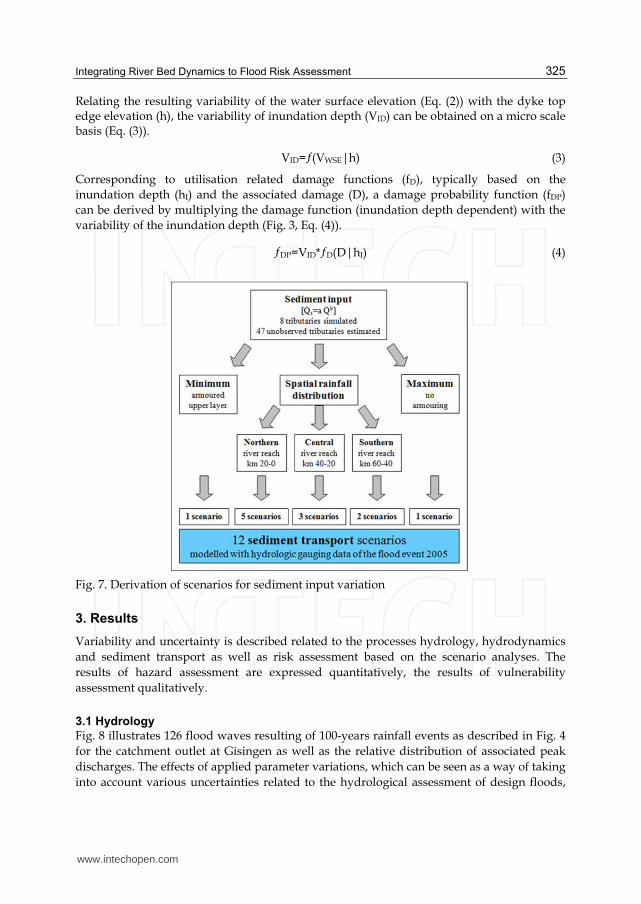
centred, southern centred and uniformly distributed – see Fig. 4) areas of high probability of sediment input are defined related to the river sections [km] 60-40, 40-20 and 20-0. For these three sections sediment input was randomly defined relying upon sediment input functions (e.g. Fig. 6) and calculated discharge rates. A minimum (armoured upper layer for all tributaries) and a maximum (no armouring for all tributaries) scenario, related to the restricting transport functions (Fig. 7), are simulated. Within these extremes, 10 scenarios were compiled by randomly drawing input capacities of each torrential inflow dependent on the magnitude of the associated flood peak in the torrential sub-catchment.

Fig. 6. Upper and lower sediment input boundary condition for the River Alfenz

To obtain realistic input distributions only one of the three sections (60-40, 40-20, 20-0) is allowed to be a dominant source of sediment input. Furthermore, to account for rainfall clusters a boundary condition for the acceptance of a randomly chosen scenario is defined: a minimum percentage of 50 % related to the section’s torrential catchment areas had to deliver maximum sediment input (i.e. potential transport rate). The 12 resulting scenarios were simulated with observed runoff data taken from the 2005 flood event with an estimated recurrence interval of 100 years.

2.3 Risk assessment Accounting for the variability of processes (hydrology, hydrodynamics and sediment transport) on a micro scale, probability distribution functions for object related inundation depths can be obtained. The variability of the water surface elevation (VWSE) is dependent on the variability of the bed elevation (VBE), as well as on the variability of the hydrologic input (VHI).

VWSE=ƒ(VBE|VHI) (2)

www.intechopen.com


Relating the resulting variability of the water surface elevation (Eq. (2)) with the dyke top edge elevation (h), the variability of inundation depth (VID) can be obtained on a micro scale basis (Eq. (3)).

VID=ƒ(VWSE|h) (3)

Corresponding to utilisation related damage functions (fD), typically based on the inundation depth (hI) and the associated damage (D), a damage probability function (fDP) can be derived by multiplying the damage function (inundation depth dependent) with the variability of the inundation depth (Fig. 3, Eq. (4)).

ƒDP=VID*ƒD(D|hI) (4)

Fig. 7. Derivation of scenarios for sediment input variation

3. Results

Variability and uncertainty is described related to the processes hydrology, hydrodynamics and sediment transport as well as risk assessment based on the scenario analyses. The results of hazard assessment are expressed quantitatively, the results of vulnerability assessment qualitatively.

3.1 Hydrology

Fig. 8 illustrates 126 flood waves resulting of 100-years rainfall events as described in Fig. 4 for the catchment outlet at Gisingen as well as the relative distribution of associated peak discharges. The effects of applied parameter variations, which can be seen as a way of taking into account various uncertainties related to the hydrological assessment of design floods,

www.intechopen.com


are shown in Table 1. Each variation of a single parameter over the full range of applied values – while keeping the others constant – yields a maximum variation in resulting runoff peaks. For a relative measure this value is related to the mean discharge of runoff peaks. The values given in Table 1 are the mean of relative peak variations for all considered scenarios. This mean relative variation shows the sensitivity of the flood simulation to changes in the respective parameter and establishes an evaluation approach for the respective uncertainty. Regarding the basin outlet at Gisingen, the spatial distribution of rainfall has the smallest impact on flood peaks. Obviously, this impact is much higher at the most-upstream gauges with a smaller catchment area (with either high or low precipitation), with relative runoff peak variations of up to 117 %. The mean variation for all Ill gauges is 41 %. Even though only three different spatial patterns are tested in this study, this shows that the importance of considering uncertainty of spatial rainfall distribution for design flood simulations depends on the spatial focus of the subsequent assessment. Other parameter variations lead to similar runoff peak variations at the basin outlet and at upstream gauges. With 11% relative runoff peak variation, changes in the temporal distribution of rainfall have a markedly lower impact on flood peaks than variations of the initial catchment conditions (27%) The variation of ARF for 12-hour storms has by far the largest effect on simulated flood hydrographs, as it directly alteres the total depth of a precipitation scenario. Storm duration, the second parameter influencing total precipitation depth cannot directly be assessed for the River Ill, because 12-hour and 24-hour storms are determined with different methods and other factors apart from duration influenced the resulting total depth. An evaluation of 2 to 12-hour storms resulting only from the mentioned meteorological convective storm model for Ill tributary sub-catchments shows mean variations in simulated runoff peaks of 20 % (Stanzel et al., 2007). In this analysis also uncertainty related to the estimation of fast runoff model parameters is investigated. Resulting runoff peak variations in tributary rivers are rather small (5 %) – as better observations are available for calibration on the River Ill, the effects of uncertainty in parameter estimation is assumed to be even smaller when regarding the entire basin.

Fig. 8. Calculated hydrographs for 100-year rainfall events and distribution of simulated peak values

www.intechopen.com


In relation to the normative 100-year design value of 820 m³/s at the gauge in Gisingen, the simulated peaks range from 45 % to 160 %. Several peaks are far below as well as over the 90 % confidence interval of statistical extreme value analyses of observed runoff, underlining that 100-year rainfall events produce flood events of different return periods. Yet, the large range of hydrographs shows how much of the possible variability of flood waves is disregarded by a design flood approach. Varied Parameter Mean variation of simulated runoff peaks at Gisingen

Spatial rainfall distribution 4 %

Temporal rainfall distribution 11 %

Initial catchment conditions 27 %

Areal reduction factor 88 %

Table 1. Sensitivity of flood peaks due to input variation for Gisingen (basin outlet)

3.2 Hydrodynamics and sediment transport

Hydrodynamic and sediment transport simulation results are illustrated exemplarily for a highly dynamic section (km 30 to 29) chosen from the considered 60 km. The selected river section is characterised by a torrential inflow located at the upper boundary. The sediment input function of this torrential inflow is documented in Fig. 6. The first 300 m of the considered reach are dominated by hydraulic structures (in- and outflow for energy generation, weir and chute) which cause spacious accumulations of sediment due to a reduction of flow velocity and accordingly to lower shear stress. In the case of higher discharge the accumulated sediment moves downstream where a dynamic river bed is encountered. In Fig.9 the modifications of river bed elevations due to hydrological and sediment input variations are illustrated. The three lines represent the maximum (dark grey), the mean (dashed grey) and the minimum (light grey) calculated bed elevation changes resulting from varying the discharge by means of 126 scenarios (Fig. 4). The inflow of the tributary immediately upstream km 30 leads to locally calculated accumulations of roughly 0.80 m. The black vertical lines indicate the station of considered cross sections and display the range of calculated bed elevation changes due to randomly selected sediment input of torrential inflows. The magnitude is based on the simulation of 12 input scenarios (Fig. 7). Fig. 10 outlines the differences (max/min) of water surface elevation and embankment elevation. Continuous lines correspond to the orographic right-hand hinterland with numerous utilisations such as private housing. Thick lines define the limits due to hydrological input variation and the thin ones, the limits due to sediment input scenarios. Corresponding to the orographic left-hand side, with no vulnerable utilisations, results are represented by grey dashed lines (thick for hydrology and thin for sediment input). The value 0.00 represents a water surface elevation equal to the dyke top edge. Overtopping occurs when displayed lines show positive values. Due to hydrologic input variation (126 scenarios – 25 % of them exceed the design water level, see Fig. 8), a high probability of overtopping is indicated. Considering sediment input variation (12 scenarios) based on discharge data of a 100-year flood (2005) only the lower part of the section is subjected to inundation. From chainage 29,100 m to 29,000 m even the

www.intechopen.com


minimum values of calculated water surface elevations lead to inundation of the flood plain. Therefore, damages have to be expected for floods lower the design value of the protection scheme (recurrence interval of 100 years, including freeboard).

Fig. 9. Changes of river bed elevations due to hydrological and sediment input variation

Fig. 10. Differences of water surface elevations and dyke top edge

3.3 Risk assessment The associated uncertainty of results obtained by design-flood-based procedures (BMFLUW, 2006 a) is emphasized by the overtopping probability caused by 138 considered scenarios (126 hydrologic scenarios, 12 sediment transport scenarios; Fig. 11). Alongside the River Ill settlements and utilisations are mainly protected by dykes and natural barriers with an estimated flood safety up to a recurrence interval of 100 years. Fig. 11 outlines the probability of overtopping along the 60 km due to variation of discharge input (126 scenarios). The calculated overtopping probability of 12.27 % indicates that 7.4 km are not protected against floods caused by 100-year rainfall events which have not been previously identified as such. In the frame of this study affected utilizations are not elaborated in detail. The analysis of the section displayed in Fig. 9 and Fig. 10 (km 30-29) proves that there are also settlements in the inundated areas.

www.intechopen.com


Referring to the results of the hydrological input variation, it has to be underlined, that considered discharges resulting from 100-year rainfall events lead to as much as 160 % of the applied design value discharge (normative 100-year flood event) for the gauge furthest downstream. Analysing scenarios by means of sediment input variation obtained by an observed 100-year flood event in the year 2005, the overtopping probability equals 1.59 % for the entire reach. Nevertheless, at 40 cross sections dykes or barriers are overtopped and therefore most likely to break.

Fig. 11. Overtopping probability and height

4. Conclusion

Integrating river bed dynamics to flood risk assessment enables a refined, more realistic, estimation of water tables and inundation lines. Obviously, uncertainty increases by including additional processes such as sudden changes of the river bed. However, the opportunity to identify related variability is provided. The presented method provides an identification of process related variability and uncertainty, considering hydrologic input generation, hydrodynamic and sediment transport. To obtain reliable results it is essential to analyse scenarios from “no damage” up to the “worst case”. State of the art approaches usually consider a small number of design flood events (in Austria: HQ30, HQ100, HQ300) to assess the overall flood risk which are usually in between “no damage” and “worst case”. Thinking about protected areas a HQ300 is by no means appropriate to assess worst case scenarios – in these cases flood risk will be under-estimated remarkably. Additionally, normatively defined scenarios usually rely upon uniform recurrence intervals of flood peaks at any location in the catchment area independent from the overall size, i.e. they disregard spatial and temporal rainfall characteristics. Therefore, the presented survey adapts state of the art approaches by

www.intechopen.com


substituting the scenario approach (a few normatively defined design floods) through a multi scenario approach by means of variation of inputs (hydrographs and sediment load). Further, vulnerability analyses and damage estimation tools were improved methodologically by interrelating the overtopping probability, the variability of inundation depth and a damage function to obtain a damage-probability relationship (Fig. 3). Hence, uncertainty and sensitivity are implicitly comprised in the probability distribution function of the expected damage. Discharge input scenarios are obtained by rainfall-runoff simulations with different 100-year rainfall events. Sediment input scenarios are simulated based on a flood event with an estimated recurrence interval of 100 years by randomly drawing loads of torrential inflows. A sensitivity analysis indicates that the discharge input variation leads to flood peaks as high as 160 % of the normative 100-year design flood. A higher probability of inundations of vulnerable utilizations like settlements, infrastructure, etc. results from discharge input variation (12.3 %) than from sediment input variations (1.6 %). Regarding the magnitude of bed elevation changes, however, the influence of sediment input variation is found to be much higher than the influence of discharge input variations. Consequently, the derivation of sediment input functions appears to be the most important task wherever the incorporation of sediment transport calculations or estimations are applicable. In this context scarce data availability seems to be the restricting factor (Nachtnebel & Neuhold, 2008). Therefore, an upgrade of continuous sediment gauges as well as the volumetric survey of accumulations, especially after flood events, is desirable. By means of an extended data base the derivation of sediment input functions as well as calibration and validation of sediment transport models would be more feasible and should be adaptable to further river types and scales. Results indicate that damage has to be assumed where safety was expected. This clearly implies that flood risk assessment approaches should be revised with respect to a multi-scenario and multi-process approach to obtain a more realistic basis for decision making.

5. References

BMFLUW (Bundesministerium für Forst- und Landwirtschaft, Umwelt und Wasserwirtschaft), 2006 a: Richtlinien zur Gefahrenzonenausweisung für die Bundeswasserbauverwaltung: Fassung 2006. Wien.

BMLFUW 2006 b: Niederschlag-Abfluss-Modellierung. Arbeitsbehelf zur Parameter-ermittlung (in German). Vienna.

Fürst, J. & Hafner, N. (2005): Land cover. In: Federal Ministry of Agriculture, Forestry, Environment and Water Management (Ed.). Hydrological Atlas of Austria, 2nd Edition. Vienna.

Geiger, H., Röthlisberger, G., Stehli, A. & Zeller, J. (2004): Extreme point rainfall of varying duration and return period. In: Swiss National Hydrological and Geological Survey (Ed.) 2004. Hydrological Atlas of Switzerland. Bern.

www.intechopen.com


Huang, J.V. & Greimann, B. (2007): US Department of Interior, Bureau of Reclamation, Technical Service Center, Sedimentation and River Hydraulics Group. User´s Manual for GSTAR-1D. 1-817.

Kling, H. (2002): Development of tools for a semi-distributed runoff model. Master thesis, IWHW BOKU, Vienna, Austria.

Larson, C.L. & Reich, B.M. (1972): Relationship of observed rainfall and runoff recurrence intervals. In: Schulz, E.F., Koelzer, V.A. and Mahmood, K., (Eds.). Floods and Droughts, Water Resources Publications, Fort Collins, pp. 34–43.

Lorenz, P. & Skoda, G. (2000): Bemessungsniederschläge kurzer Dauerstufen (D ≤ 12 Stunden) mit inadäquaten Daten (in German). Report of the hydrographical service in Austria, Nr. 80, Vienna.

Meyer-Peter, E. & Müller, R. (1948): “Formula for bed-load transport” Proc. of the Int. Assoc. for Hydraulic Research, 2nd Meeting, Stockholm.

Nachtnebel, H.P., Baumung, S. & Lettl, W. (1993): Abflussprognosemodell für das Einzugsgebiet der Enns und Steyr (in German). Report, IWHW, BOKU Austria.

Nachtnebel, H.P. & Debene, A. (2004):“Schwebstoffbilanzierung im Bereich von Stauräumen an der österr. Donau“. FloodRisk: Endbericht im Auftrag des Lebensministeriums. In: Habersack H., Bürgel J. and Petraschek A.: Analyse der Hochwasserereignisse vom August 2002- Flood Risk, 2004, BMLFUW, Wien, Österreich.

Nachtnebel, H.P. & Neuhold, C. (2008): Schutzwasserbauliche Bestandserhebung Ill, Arbeitspaket 5: Hydraulik/Geschiebe/Schwebstoffe. IWHW, Wien.

Nash, J.E. & Sutcliffe, J.V. (1970): River Flow Forecasting through Conceptual Models. Journal of Hydrology, 10 / 3.

Neuhold, C.; Stanzel, P. & Nachtnebel, H.P. (2007): Modelling morphological changes during flood events utilised as impact on flood risk assessment. In: European Geosciences Union, Geophysical Research Abstracts, Volume 9.

Neuhold, C.; Stanzel, P. & Nachtnebel H.P. (2009): Incorporating river morphological changes to flood risk assessment: uncertainties, methodology and application. Nat. Hazards and Earth Syst. Sci., 9, 789-799

Neuhold, C.; Stanzel, P. & Nachtnebel H.P. (2010 a): Integrating river bed dynamics to flood risk assessment. In: Nachtnebel H.P.; Cruz, A.M.; Amendola, A.; Mechler, R. & Tatano, H. (Eds). Abstract-Volume: 1st Annual Conference of the International Society for Integrated Disaster Risk Management – IDRiM 2010

Neuhold, C.; Stanzel, P. & Nachtnebel H.P. (2010 b): Analysing uncertainties associated with flood hazard assessment. In: EGU, Geophysical Research Abstracts, Volume 12.

Neuhold, C. & Nachtnebel, H.P. (2011): Assessing flood risk associated with waste disposals: methodology, application and uncertainties. Nat Hazards 56:359-370

Peticzka, P. & Kriz, K. (2005): General soil map. In: Federal Ministry of Agriculture, Forestry, Environment and Water Management (Ed.). Hydrological Atlas of Austria, 2nd Edition. Vienna.

Skoda, G., Weilguni, V. & Haiden, T. (2005): Heavy Convective Storms – Precipitation during 15, 60 und 180 minutes. In: BMFLUW (Ed.) 2005. Hydrological Atlas of Austria, 2nd Edition. Vienna.

www.intechopen.com


Stanzel, P., Neuhold, C. & Nachtnebel, H.P. (2007): Estimation of design floods for ungauged basins in an alpine watershed. In: EGU, Geophysical Research Abstracts, Volume 9.

www.intechopen.com

Sediment Transport in Aquatic EnvironmentsEdited by Dr. Andrew Manning

ISBN 978-953-307-586-0Hard cover, 332 pagesPublisher InTechPublished online 30, September, 2011Published in print edition September, 2011

InTech EuropeUniversity Campus STeP Ri Slavka Krautzeka 83/A 51000 Rijeka, Croatia Phone: +385 (51) 770 447 Fax: +385 (51) 686 166www.intechopen.com

InTech ChinaUnit 405, Office Block, Hotel Equatorial Shanghai No.65, Yan An Road (West), Shanghai, 200040, China

Phone: +86-21-62489820 Fax: +86-21-62489821

Sediment Transport in Aquatic Environments is a book which covers a wide range of topics. The effectivemanagement of many aquatic environments, requires a detailed understanding of sediment dynamics. Thishas both environmental and economic implications, especially where there is any anthropogenic involvement.Numerical models are often the tool used for predicting the transport and fate of sediment movement in thesesituations, as they can estimate the various spatial and temporal fluxes. However, the physical sedimentaryprocesses can vary quite considerably depending upon whether the local sediments are fully cohesive, non-cohesive, or a mixture of both types. For this reason for more than half a century, scientists, engineers,hydrologists and mathematicians have all been continuing to conduct research into the many aspects whichinfluence sediment transport. These issues range from processes such as erosion and deposition to howsediment process observations can be applied in sediment transport modeling frameworks. This book reportsthe findings from recent research in applied sediment transport which has been conducted in a wide range ofaquatic environments. The research was carried out by researchers who specialize in the transport ofsediments and related issues. I highly recommend this textbook to both scientists and engineers who deal withsediment transport issues.

How to referenceIn order to correctly reference this scholarly work, feel free to copy and paste the following:

Clemens Neuhold, Philipp Stanzel and Hans Peter Nachtnebel (2011). Integrating River Bed Dynamics toFlood Risk Assessment, Sediment Transport in Aquatic Environments, Dr. Andrew Manning (Ed.), ISBN: 978-953-307-586-0, InTech, Available from: http://www.intechopen.com/books/sediment-transport-in-aquatic-environments/integrating-river-bed-dynamics-to-flood-risk-assessment

8:; ' # '7& *#8 & 9cdn.intechopen.com/pdfs-wm/20923.pdf · integrating river bed...

Documents