74 th eage conference & exhibition incorporating spe europec 2012 automated seismic-to-well...
TRANSCRIPT

74th EAGE Conference & Exhibition incorporating SPE EUROPEC 2012
Automated seismic-to-well ties?
Roberto H. Herrera and Mirko van der Baan University of Alberta, Edmonton, Canada
Outline• Introduction• Similarity in time series• The manual seismic-to-well tie• What is Dynamic Time Warping
– How DTW works?– The automated approach
• Real examples– Manual vs Automatic
• Conclusions

Seismic-to-well similarity
• Objective:– Can you automate the seismic-to-well tie?
• Possible applications: – Seismic-to-well tie, log-to-log correlation,
alignment of baseline + monitor in 4D • Main problem
– Bulk shift, stretching and squeezing is an interpretation item.
–How to implement semi-automatically?

Similarity vs Correlation

How similar are they?

How similar are they?
500 1000 1500 2000-1012
Shapes to Signals
500 1000 1500 2000
-1012
500 1000 1500 2000
-1012
500 1000 1500 2000
-1012
Samples
-2000 -1000 0 1000 2000
0
0.5
1Cross-Correlation
-2000 -1000 0 1000 2000-0.2
00.20.40.60.8
-2000 -1000 0 1000 2000-0.5
0
0.5
-2000 -1000 0 1000 2000-0.2
00.20.40.60.8
Lag Samples
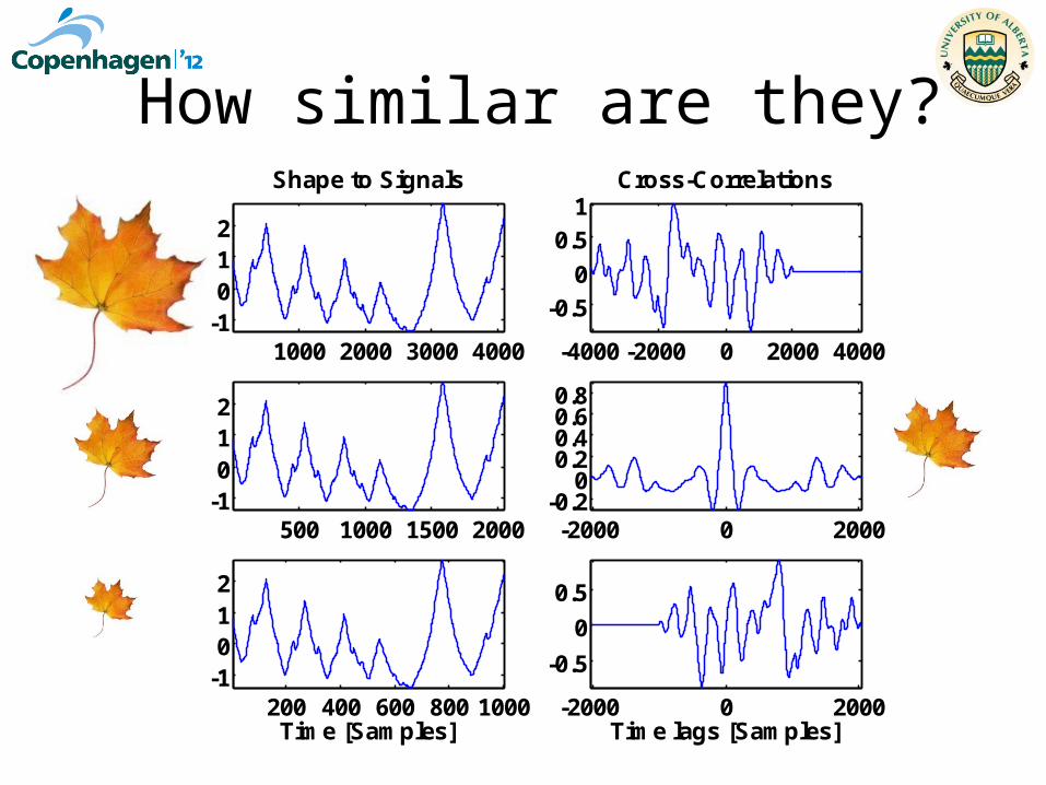
How similar are they?
1000 2000 3000 4000-1012
Shape to Signals
500 1000 1500 2000-1012
200 400 600 800 1000-1012
Time [Samples]
-4000 -2000 0 2000 4000
-0.5
0
0.5
1Cross-Correlations
-2000 0 2000-0.2
00.20.40.60.8
-2000 0 2000
-0.5
0
0.5
Time lags [Samples]
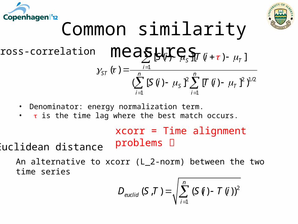
Common similarity measuresCross-correlation
1
2 2 1/2
1 1
[ ( ) ][ ( ) ]( )
( [ ( ) ] [ ( ) ] )
n
S Ti
ST n n
S Ti i
S i T i
S i T i
• Denominator: energy normalization term.• is the time lag where the best match occurs.
xcorr = Time alignment problems
An alternative to xcorr (L_2-norm) between the two time series
2
1
( , ) ( ( ) ( ))n
euclidi
D S T S i T i
Euclidean distance
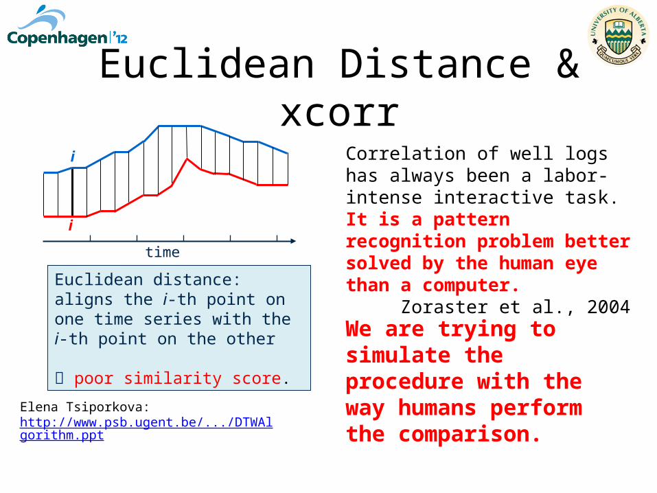
Euclidean Distance & xcorr
i
i
time
Euclidean distance:aligns the i-th point on one time series with the i-th point on the other
poor similarity score.
Correlation of well logs has always been a labor-intense interactive task. It is a pattern recognition problem better solved by the human eye than a computer.
Zoraster et al., 2004
We are trying to simulate the procedure with the way humans perform the comparison.Elena Tsiporkova:
http://www.psb.ugent.be/.../DTWAlgorithm.ppt

The forward model
Sonic logP-waveVp
Well logs
Bulk densityρ
AcousticImpedanceI
1
1
i ii
i i
I IR
I I
Reflectivityr
Computed
StatisticalWavelet
Waveletw
Convolution output
Synthetics

Experiments
Xline 42
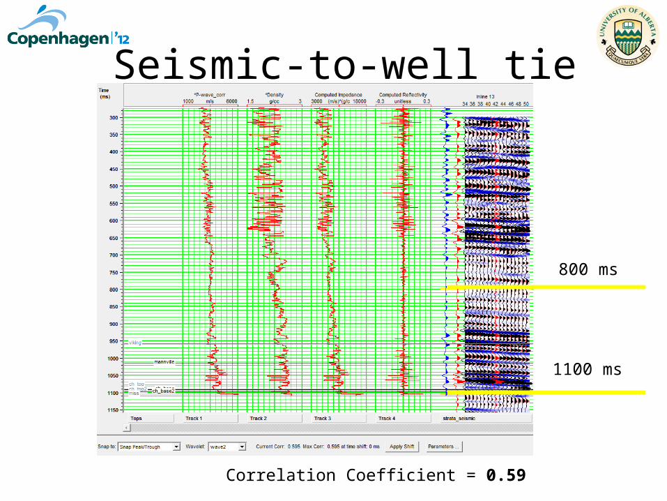
Seismic-to-well tie
Correlation Coefficient = 0.59
800 ms
1100 ms

600 ms
1100 ms
Correlation Coefficient = 0.40
Seismic-to-well tie

Seismic-to-well tie
Correlation Coefficient = 0.148 and could be 0.45 with 25 ms of time shift
600 ms
900 ms
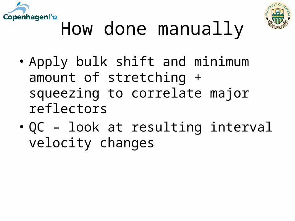
How done manually
• Apply bulk shift and minimum amount of stretching + squeezing to correlate major reflectors
• QC – look at resulting interval velocity changes

Dynamic Time Warping?
i
i+2
i
i i
timetime
Euclidean distance:aligns the i-th point on one time series with the i-th point on the other
poor similarity score.
DTW: A non-linear (elastic) alignment:produces a more intuitive similarity measure.It matches similar shapes even if they are out of phase on the time axis.
A pattern matching technique that is“visually perceptive and intuitive”
Elena Tsiporkova: http://www.psb.ugent.be/cbd/papers/gentxwarper/DTWAlgorithm.ppt
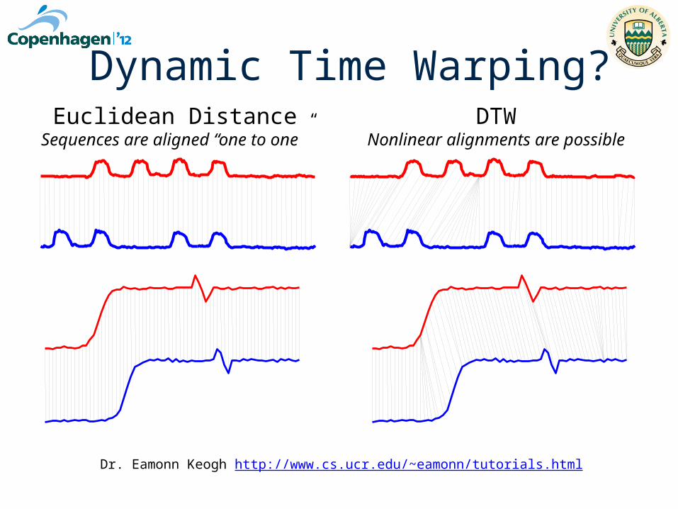
Dynamic Time Warping?Euclidean Distance
Sequences are aligned “one to one”DTW
Nonlinear alignments are possible
Dr. Eamonn Keogh http://www.cs.ucr.edu/~eamonn/tutorials.html
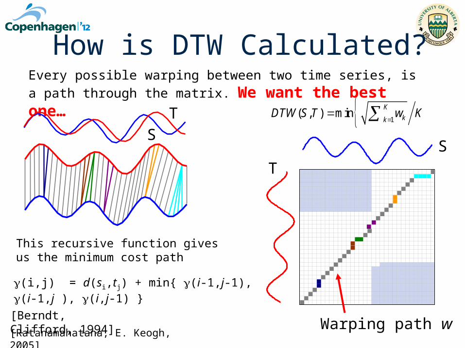
How is DTW Calculated?
[Ratanamahatana, E. Keogh, 2005]
Every possible warping between two time series, is a path through
the matrix. We want the best one…
ST 1
( , ) minK
kkDTW S T w K
T
Warping path w
S
This recursive function gives us the minimum cost path
(i,j) = d(si,tj) + min{ (i-1,j-1), (i-1,j ), (i,j-1) }
[Berndt, Clifford, 1994]
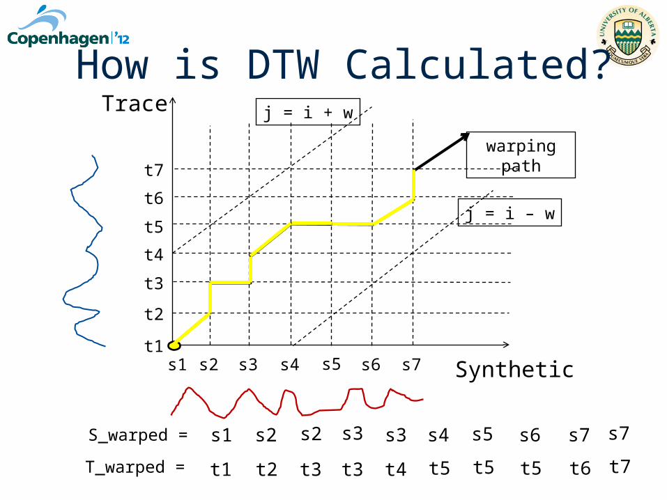
How is DTW Calculated?
Synthetic
Trace
warping path
j = i – w
j = i + w
s1 s2 s3t1
s4 s5 s6 s7
t2
t3
t4
t5
t6
t7
S_warped = s1 s2 s2 s3 s3
t1 t2 t3 t3 t4T_warped =
s4
t5
s5
t5
s6
t5
s7
t6
s7
t7
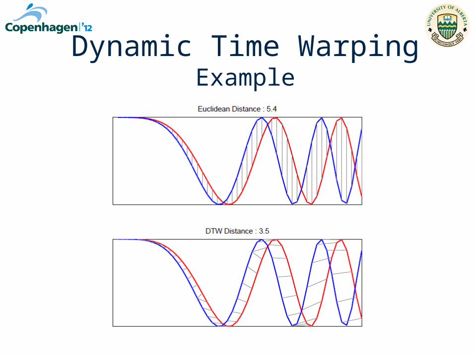
Dynamic Time WarpingExample

Dynamic Time Warping
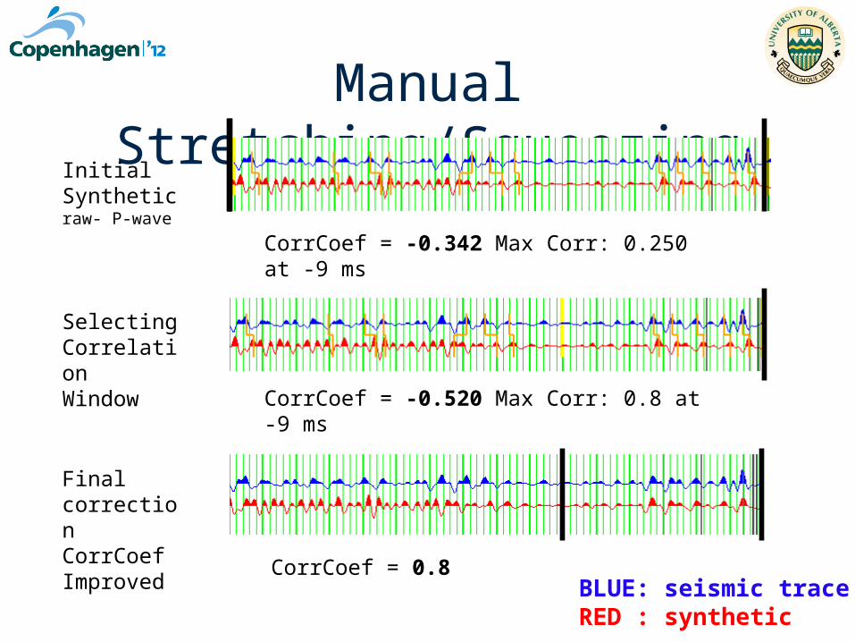
Manual Stretching/Squeezing
InitialSyntheticraw- P-wave
SelectingCorrelationWindow
Final correctionCorrCoefImproved
CorrCoef = -0.342 Max Corr: 0.250 at -9 ms
CorrCoef = -0.520 Max Corr: 0.8 at -9 ms
CorrCoef = 0.8BLUE: seismic traceRED : synthetic
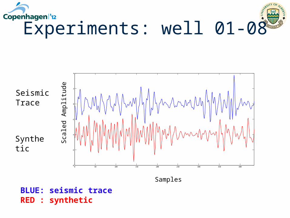
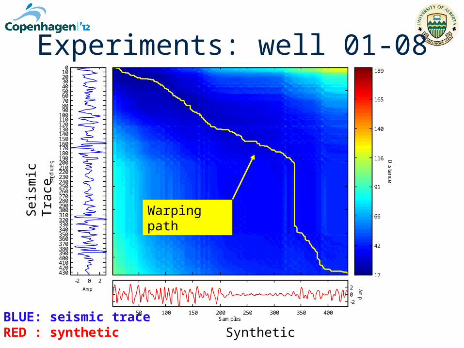
Experiments: well 01-08
Seismic Trace
Synthetic
0 50 100 150 200 250 300 350 400-8
-6
-4
-2
0
2
4
Samples
Sca
led
Am
plitu
de
BLUE: seismic traceRED : synthetic
Experiments: well 01-08S
eis
mic
Tra
ce
SyntheticBLUE: seismic traceRED : synthetic
Dis
tance
17
42
66
91
116
140
165
189
-2 0 2
430420410400390380370360350340330320310300290280270260250240230220210200190180170160150140130120110100
908070605040302010
0
Sam
ples
Amp
50 100 150 200 250 300 350 400
-202
Samples
Am
p
Warping path

Experiments: well 01-08
Seismic Trace
Synthetic
0 50 100 150 200 250 300 350 400-8
-6
-4
-2
0
2
4
Samples
Sca
led
Am
plitu
de
BLUE: seismic traceRED : synthetic

Bounded - DTW
Synthetic
Trace
warping path
j = i – w
j = i + w
s1 s2 s3t1
s4 s5 s6 s7
t2
t3
t4
t5
t6
t7
S_warped = s1 s2 s2 s3 s3
t1 t2 t3 t3 t4T_warped =
s4
t5
s5
t5
s6
t5
s7
t6
s7
t7

Se
ism
ic T
race
Synthetic
Dista
nce
0
20
39
59
79
98
118
138
-2 0 243042041040039038037036035034033032031030029028027026025024023022021020019018017016015014013012011010090 80 70 60 50 40 30 20 10 0
Sa
mp
les
Amp
50 100 150 200 250 300 350 400-2
0
2
4
Samples
Am
p
Experiments: well 01-08S
eis
mic
Tra
ce
Synthetic
Warping path
BLUE: seismic traceRED : synthetic

Experiments: well 01-08
50 100 150 200 250 300 350 400-1
-0.5
0
0.5
1Original signals. Synthetic (red) and Seismic Trace (blue)
No
rma
lize
d A
mp
litu
de
Samples
100 200 300 400 500 600
-3
-2
-1
0
1
2
3
4
Warped signals. Synthetic (red) and Seismic Trace (blue)
No
rma
lize
d A
mp
litu
de
Samples
BLUE: seismic traceRED : synthetic
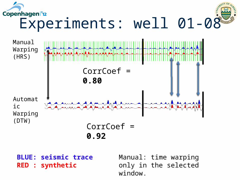
Experiments: well 01-08ManualWarping(HRS)
AutomaticWarping(DTW)
BLUE: seismic traceRED : synthetic
Manual: time warping only in the selected window.
CorrCoef = 0.92
CorrCoef = 0.80

Warping path: well 16-08S
eis
mic
Tra
ce
SyntheticBLUE: seismic traceRED : synthetic
Dis
tan
ce
1
20
39
57
76
95
114
132
-2 0 2
430
420
410
400
390
380
370
360
350
340
330
320
310
300
290
280
270
260
250
240
230
220
210
200
190
180
170
160
150
140
130
120
110
100
90
80
70
60
50
40
30
20
10
0
Sa
mp
les
Amp
50 100 150 200 250 300 350 400
-2
0
2
4
Samples
Am
p

Automatic stretch/squeeze: well 16-08
50 100 150 200 250 300 350 400-1
-0.5
0
0.5
1Original signals. Synthetic (red) and Seismic Trace (blue)
No
rma
lize
d A
mp
litu
de
Samples
100 200 300 400 500 600-3
-2
-1
0
1
2
3
4
Warped signals. Synthetic (red) and Seismic Trace (blue)
No
rma
lize
d A
mp
litu
de
Samples
BLUE: seismic traceRED : synthetic
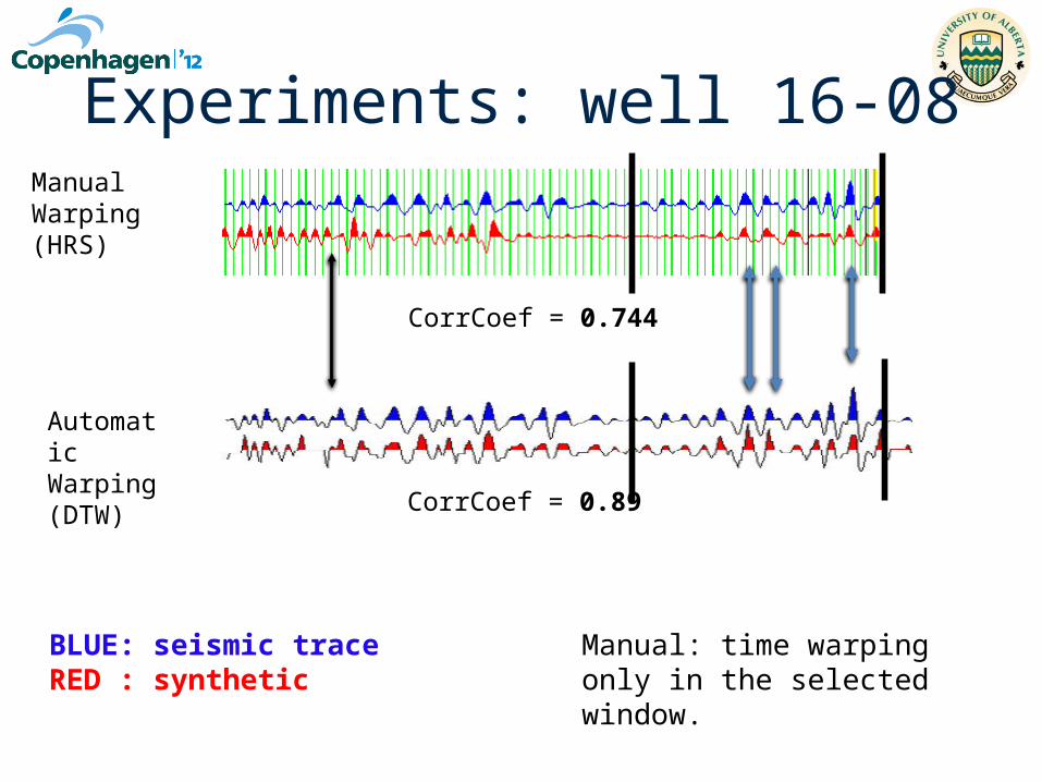
Experiments: well 16-08 ManualWarping(HRS)
AutomaticWarping(DTW)
BLUE: seismic traceRED : synthetic
Manual: time warping only in the selected window.
CorrCoef = 0.89
CorrCoef = 0.744

Discussion
• Pros and cons– Independent of the selected window.– Able to follow non linearities
– Only intended as a guide – not all stretching-squeezing is realistic
– QC – examine changes in resulting interval velocity curve

Conclusions• DTW: optimal solution for matching similar events. • DTW: complementary tool for seismic-to-well tie.• Many other applications of DTW are possible for seismic data.
– log-to-log correlations, alignment of baseline and monitor surveys in 4D seismics, PP and PS wavefield registration for 3C data.
BLISS sponsors
BLind Identification of Seismic Signals (BLISS) is supported by
Hampson-Russell for software licensing
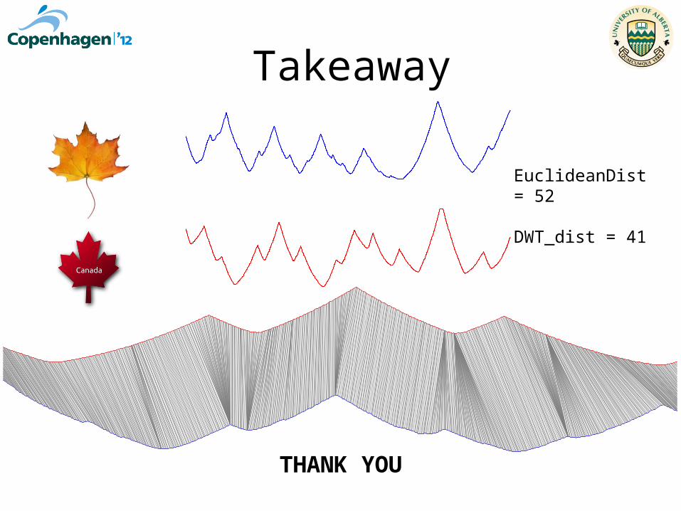
Takeaway
EuclideanDist = 52
DWT_dist = 41
THANK YOU