7.1 introducingrationalfunctions - college of the...

Section 7.1 Introducing Rational Functions 603

Version: Fall 2007

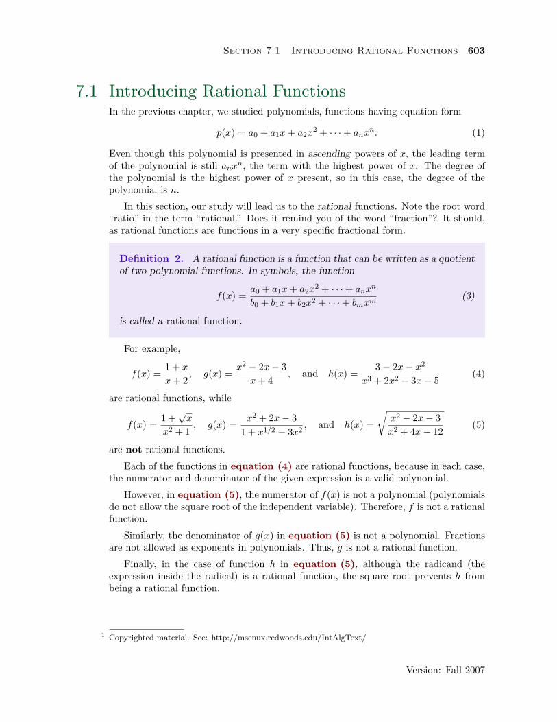
7.1 Introducing Rational FunctionsIn the previous chapter, we studied polynomials, functions having equation form

p(x) = a0 + a1x+ a2x2 + · · ·+ anxn. (1)

Even though this polynomial is presented in ascending powers of x, the leading termof the polynomial is still anxn, the term with the highest power of x. The degree ofthe polynomial is the highest power of x present, so in this case, the degree of thepolynomial is n.

In this section, our study will lead us to the rational functions. Note the root word“ratio” in the term “rational.” Does it remind you of the word “fraction”? It should,as rational functions are functions in a very specific fractional form.

Definition 2. A rational function is a function that can be written as a quotientof two polynomial functions. In symbols, the function

f(x) = a0 + a1x+ a2x2 + · · ·+ anxn

b0 + b1x+ b2x2 + · · ·+ bmxm(3)

is called a rational function.

For example,

f(x) = 1 + xx+ 2

, g(x) = x2 − 2x− 3x+ 4

, and h(x) = 3− 2x− x2

x3 + 2x2 − 3x− 5(4)

are rational functions, while

f(x) = 1 +√x

x2 + 1, g(x) = x2 + 2x− 3

1 + x1/2 − 3x2 , and h(x) =√x2 − 2x− 3x2 + 4x− 12

(5)

are not rational functions.Each of the functions in equation (4) are rational functions, because in each case,

the numerator and denominator of the given expression is a valid polynomial.However, in equation (5), the numerator of f(x) is not a polynomial (polynomials

do not allow the square root of the independent variable). Therefore, f is not a rationalfunction.

Similarly, the denominator of g(x) in equation (5) is not a polynomial. Fractionsare not allowed as exponents in polynomials. Thus, g is not a rational function.

Finally, in the case of function h in equation (5), although the radicand (theexpression inside the radical) is a rational function, the square root prevents h frombeing a rational function.

Copyrighted material. See: http://msenux.redwoods.edu/IntAlgText/1

604 Chapter 7 Rational Functions

Version: Fall 2007

An important skill to develop is the ability to draw the graph of a rational function.Let’s begin by drawing the graph of one of the simplest (but most fundamental) rationalfunctions.

The Graph of y = 1/xIn all new situations, when we are presented with an equation whose graph we’ve notconsidered or do not recognize, we begin the process of drawing the graph by creatinga table of points that satisfy the equation. It’s important to remember that the graphof an equation is the set of all points that satisfy the equation. We note that zero isnot in the domain of y = 1/x (division by zero makes no sense and is not defined), andcreate a table of points satisfying the equation shown in Figure 1.

x10

y10

x y = 1/x−3 −1/3−2 −1/2−1 −11 12 1/23 1/3

Figure 1. At the right is a table of points satisfying the equation y =1/x. These points are plotted as solid dots on the graph at the left.

At this point (see Figure 1), it’s pretty clear what the graph is doing betweenx = −3 and x = −1. Likewise, it’s clear what is happening between x = 1 and x = 3.However, there are some open areas of concern.

1. What happens to the graph as x increases without bound? That is, what happensto the graph as x moves toward ∞?

2. What happens to the graph as x decreases without bound? That is, what happensto the graph as x moves toward −∞?

3. What happens to the graph as x approaches zero from the right?4. What happens to the graph as x approaches zero from the left?

Let’s answer each of these questions in turn. We’ll begin by discussing the “end-behavior” of the rational function defined by y = 1/x. First, the right end. Whathappens as x increases without bound? That is, what happens as x increases toward∞? In Table 1(a), we computed y = 1/x for x equalling 100, 1 000, and 10 000. Notehow the y-values in Table 1(a) are all positive and approach zero.

Students in calculus use the following notation for this idea.

limx→∞y = lim

x→∞

1x

= 0 (6)


Version: Fall 2007

They say “the limit of y as x approaches infinity is zero.” That is, as x approachesinfinity, y approaches zero.

x y = 1/x100 0.01

1 000 0.00110 000 0.0001

x y = 1/x−100 −0.01−1 000 −0.001−10 000 −0.0001

(a) (b)Table 1. Examining the end-behavior of y = 1/x.

A completely similar event happens at the left end. As x decreases without bound,that is, as x decreases toward −∞, note that the y-values in Table 1(b) are all negativeand approach zero. Calculus students have a similar notation for this idea.

limx→−∞

y = limx→−∞

1x

= 0. (7)

They say “the limit of y as x approaches negative infinity is zero.” That is, as xapproaches negative infinity, y approaches zero.

These numbers in Tables 1(a) and 1(b), and the ideas described above, predict thecorrect end-behavior of the graph of y = 1/x. At each end of the x-axis, the y-valuesmust approach zero. This means that the graph of y = 1/x must approach the x-axisfor x-values at the far right- and left-ends of the graph. In this case, we say that thex-axis acts as a horizontal asymptote for the graph of y = 1/x. As x approaches eitherpositive or negative infinity, the graph of y = 1/x approaches the x-axis. This behavioris shown in Figure 2.

x10

y10

Figure 2. The graph of 1/x ap-proaches the x-axis as x increases ordecreases without bound.

Our last investigation will be on the interval from x = −1 to x = 1. Readers areagain reminded that the function y = 1/x is undefined at x = 0. Consequently, we willbreak this region in half, first investigating what happens on the region between x = 0


Version: Fall 2007

and x = 1. We evaluate y = 1/x at x = 1/2, x = 1/4, and x = 1/8, as shown in thetable in Figure 3, then plot the resulting points.

x10

y10

x y = 1/x1/2 21/4 41/8 8


Note that the x-values in the table in Figure 3 approach zero from the right, thennote that the corresponding y-values are getting larger and larger. We could continuein this vein, adding points. For example, if x = 1/16, then y = 16. If x = 1/32, theny = 32. If x = 1/64, then y = 64. Each time we halve our value of x, the resultingvalue of x is closer to zero, and the corresponding y-value doubles in size. Calculusstudents describe this behavior with the notation

limx→0+

y = limx→0+

1x

=∞. (8)

That is, as “x approaches zero from the right, the value of y grows to infinity.” This isevident in the graph in Figure 3, where we see the plotted points move closer to thevertical axis while at the same time moving upward without bound.

A similar thing happens on the other side of the vertical axis, as shown in Figure 4.

x10

y10

x y = 1/x−1/2 −2−1/4 −4−1/8 −8



Version: Fall 2007

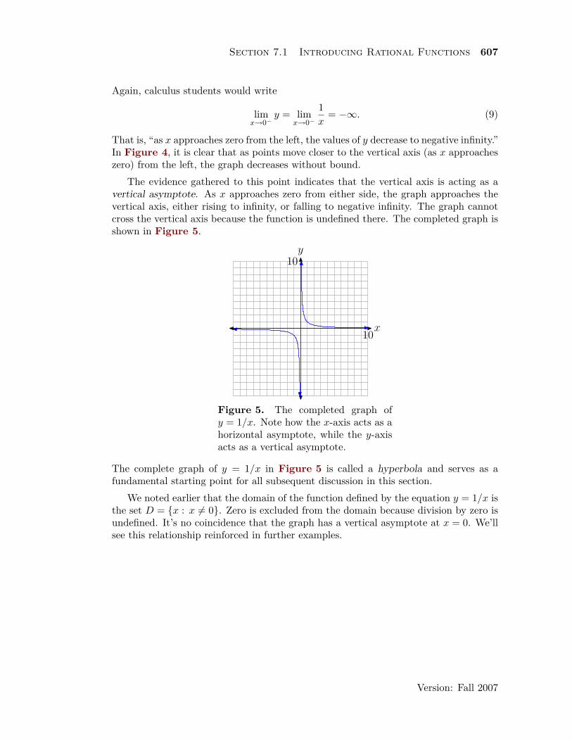
Again, calculus students would write

limx→0−

y = limx→0−

1x

= −∞. (9)

That is, “as x approaches zero from the left, the values of y decrease to negative infinity.”In Figure 4, it is clear that as points move closer to the vertical axis (as x approacheszero) from the left, the graph decreases without bound.

The evidence gathered to this point indicates that the vertical axis is acting as avertical asymptote. As x approaches zero from either side, the graph approaches thevertical axis, either rising to infinity, or falling to negative infinity. The graph cannotcross the vertical axis because the function is undefined there. The completed graph isshown in Figure 5.

x10

y10

Figure 5. The completed graph ofy = 1/x. Note how the x-axis acts as ahorizontal asymptote, while the y-axisacts as a vertical asymptote.

The complete graph of y = 1/x in Figure 5 is called a hyperbola and serves as afundamental starting point for all subsequent discussion in this section.

We noted earlier that the domain of the function defined by the equation y = 1/x isthe set D = {x : x 6= 0}. Zero is excluded from the domain because division by zero isundefined. It’s no coincidence that the graph has a vertical asymptote at x = 0. We’llsee this relationship reinforced in further examples.


Version: Fall 2007

TranslationsIn this section, we will translate the graph of y = 1/x in both the horizontal and verticaldirections.

I Example 10. Sketch the graph of

y = 1x+ 3

− 4. (11)

Technically, the function defined by y = 1/(x + 3) − 4 does not have the generalform (3) of a rational function. However, in later chapters we will show how y =1/(x+ 3)− 4 can be manipulated into the general form of a rational function.

We know what the graph of y = 1/x looks like. If we replace x with x+ 3, this willshift the graph of y = 1/x three units to the left, as shown in Figure 6(a). Note thatthe vertical asymptote has also shifted 3 units to the left of its original position (they-axis) and now has equation x = −3. By tradition, we draw the vertical asymptoteas a dashed line.

If we subtract 4 from the result in Figure 6(a), this will shift the graph in Figure 6(a)four units downward to produce the graph shown in Figure 6(b). Note that the hori-zontal asymptote also shifted 4 units downward from its original position (the x-axis)and now has equation y = −4.

x10

y10x = −3

x10

y10x = −3

y = −4

(a) y = 1/(x + 3) (b) y = 1/(x + 3) − 4Figure 6. Shifting the graph of y = 1/x.

If you examine equation (11), you note that you cannot use x = −3 as this willmake the denominator of equation (11) equal to zero. In Figure 6(b), note thatthere is a vertical asymptote in the graph of equation (11) at x = −3. This is acommon occurrence, which will be a central theme of this chapter.


Version: Fall 2007

Let’s ask another key question.

I Example 12. What are the domain and range of the rational function presentedin Example 10?

You can glance at the equation

y = 1x+ 3

− 4

of Example 10 and note that x = −3 makes the denominator zero and must beexcluded from the domain. Hence, the domain of this function is D = {x : x 6= −3}.

However, you can also determine the domain by examining the graph of the functionin Figure 6(b). Note that the graph extends indefinitely to the left and right. Onemight first guess that the domain is all real numbers if it were not for the verticalasymptote at x = −3 interrupting the continuity of the graph. Because the graph ofthe function gets arbitrarily close to this vertical asymptote (on either side) withoutactually touching the asymptote, the graph does not contain a point having an x-valueequaling −3. Hence, the domain is as above, D = {x : x 6= −3}. This is comforting thatthe graphical analysis agrees with our earlier analytical determination of the domain.

The graph is especially helpful in determining the range of the function. Note thatthe graph rises to positive infinity and falls to negative infinity. One would first guessthat the range is all real numbers if it were not for the horizontal asymptote at y = −4interrupting the continuity of the graph. Because the graph gets arbitrarily close tothe horizontal asymptote (on either side) without actually touching the asymptote, thegraph does not contain a point having a y-value equaling −4. Hence, −4 is excludedfrom the range. That is, R = {y : y 6= −4}.

Scaling and ReflectionIn this section, we will both scale and reflect the graph of y = 1/x. For extra measure,we also throw in translations in the horizontal and vertical directions.

I Example 13. Sketch the graph of

y = − 2x− 4

+ 3. (14)

First, we multiply the equation y = 1/x by −2 to get

y = −2x.

Multiplying by 2 should stretch the graph in the vertical directions (both positive andnegative) by a factor of 2. Note that points that are very near the x-axis, when doubled,are not going to stray too far from the x-axis, so the horizontal asymptote will remainthe same. Finally, multiplying by −2 will not only stretch the graph, it will also reflectthe graph across the x-axis, as shown in Figure 7(b).2

Recall that we saw similar behavior when studying the parabola. The graph of y = −2x2 stretched2

(vertically) the graph of the equation y = x2 by a factor of 2, then reflected the result across the x-axis.


Version: Fall 2007

x10

y10

x10

y10

(a) y = 1/x (b) y = −2/xFigure 7. Scaling and reflecting the graph of y = 1/x.

Replacing x with x− 4 will shift the graph 4 units to the right, then adding 3 willshift the graph 3 units up, as shown in Figure 8. Note again that x = 4 makes thedenominator of y = −2/(x− 4) + 3 equal to zero and there is a vertical asymptote atx = 4. The domain of this function is D = {x : x 6= 4}.

As x approaches positive or negative infinity, points on the graph of y = −2/(x−4)+3 get arbitrarily close to the horizontal asymptote y = 3 but never touch it. Therefore,there is no point on the graph that has a y-value of 3. Thus, the range of the functionis the set R = {y : y 6= 3}.

x10

y10 x = 4

y = 3

Figure 8. The graph of y = −2/(x −4) + 3 is shifted 4 units right and 3 unitsup.


Version: Fall 2007

Difficulties with the Graphing CalculatorThe graphing calculator does a very good job drawing the graphs of “continuous func-tions.”

A continuous function is one that can be drawn in one continuous stroke, neverlifting pen or pencil from the paper during the drawing.

Polynomials, such as the one in Figure 9, are continuous functions.

x10

y50

Figure 9. A polynomial is a continu-ous function.

Unfortunately, a rational function with vertical asymptote(s) is not a continuous func-tion. First, you have to lift your pen at points where the denominator is zero, becausethe function is undefined at these points. Secondly, it’s not uncommon to have tojump from positive infinity to negative infinity (or vice-versa) when crossing a verticalasymptote. When this happens, we have to lift our pen and shift it before continuingwith our drawing.

However, the graphing calculator does not know how to do this “lifting” of the pennear vertical asymptotes. The graphing calculator only knows one technique, plot apoint, then connect it with a segment to the last point plotted, move an incrementaldistance and repeat. Consequently, when the graphing calculator crosses a verticalasymptote where there is a shift from one type of infinity to another (e.g., from positiveto negative), the calculator draws a “false line” of connection, one that it should notdraw. Let’s demonstrate this aberration with an example.

I Example 15. Use a graphing calculator to draw the graph of the rational functionin Example 13.

Load the equation into your calculator, as shown in Figure 10(a). Set the windowas shown in Figure 10(b), then push the GRAPH button to draw the graph shown inFigure 10(c). Results may differ on some calculators, but in our case, note the “false


Version: Fall 2007

line” drawn from the top of the screen to the bottom, attempting to “connect” the twobranches of the hyperbola.

Some might rejoice and claim, “Hey, my graphing calculator draws vertical as-ymptotes.” However, before you get too excited, note that in Figure 8 the verticalasymptote should occur at exactly x = 4. If you look very carefully at the “verticalline” in Figure 10(c), you’ll note that it just misses the tick mark at x = 4. This “ver-tical line” is a line that the calculator should not draw. The calculator is attemptingto draw a continuous function where one doesn’t exist.

(a) (b) (c)Figure 10. The calculator attempts to draw a continuous function when it shouldn’t.

One possible workaround3 is to press the MODE button on your keyboard, whichopens the menu shown in Figure 11(a). Use the arrow keys to highlight DOT insteadof CONNECTED and press the ENTER key to make the selection permanent. Press theGRAPH button to draw the graph in Figure 11(b).

(a) (b)Figure 11. The same graph in “dot mode.”

This “dot mode” on your calculator calculates the next point on the graph and plotsthe point, but it does not connect it with a line segment to the previously plottedpoint. This mode is useful in demonstrating that the vertical line in Figure 10(c) isnot really part of the graph, but we lose some parts of the graph we’d really like to see.Compromise is in order.

This example clearly shows that intelligent use of the calculator is a required com-ponent of this course. The calculator is not simply a “black box” that automaticallydoes what you want it to do. In particular, when you are drawing rational functions,it helps to know ahead of time the placement of the vertical asymptotes. Knowledge

Instructors might discuss a number of alternative strategies to represent rational functions on the3

graphing calculator. What we present here is only one of a number of approaches.


Version: Fall 2007

of the asymptotes, coupled with what you see on your calculator screen, should enableyou to draw a graph as accurate as that shown in Figure 8.

Gentle reminder. You’ll want to set your calculator back in “connected mode.”To do this, press the MODE button on your keyboard to open the menu in Figure 10(a)once again. Use your arrow keys to highlight CONNECTED, then press the ENTER key tomake the selection permanent.

7.1 introducingrationalfunctions - college of the...

Documents