7 advanced database systems - cmu 15-721
TRANSCRIPT
Le
ctu
re #
17
Parallel Join Algorithms(Hashing)@Andy_Pavlo // 15-721 // Spring 2020
ADVANCEDDATABASE SYSTEMS

15-721 (Spring 2020)
Background
Parallel Hash Join
Hash Functions
Hashing Schemes
Evaluation
2
15-721 (Spring 2020)
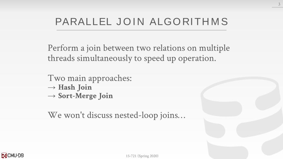
PARALLEL JOIN ALGORITHMS
Perform a join between two relations on multiple threads simultaneously to speed up operation.
Two main approaches:→ Hash Join→ Sort-Merge Join
We won't discuss nested-loop joins…
3
15-721 (Spring 2020)
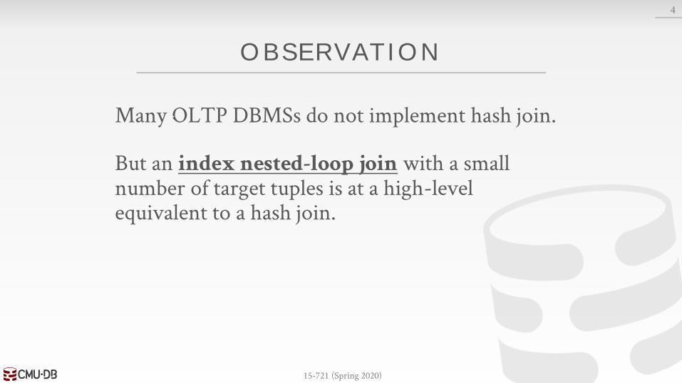
OBSERVATION
Many OLTP DBMSs do not implement hash join.
But an index nested-loop join with a small number of target tuples is at a high-level equivalent to a hash join.
4
15-721 (Spring 2020)
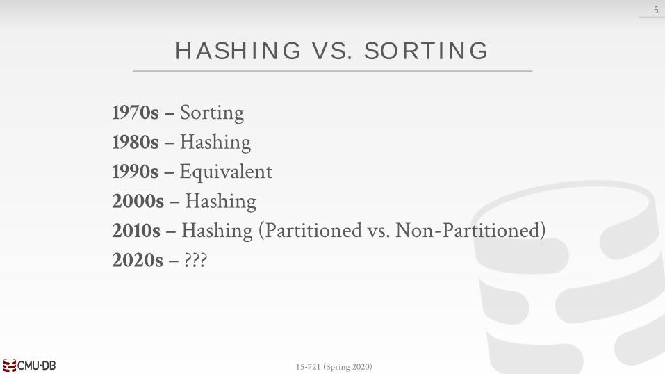
HASHING VS. SORTING
1970s – Sorting
1980s – Hashing
1990s – Equivalent
2000s – Hashing
2010s – Hashing (Partitioned vs. Non-Partitioned)
2020s – ???
5

15-721 (Spring 2020)
PARALLEL JOIN ALGORITHMS
6
→ Hashing is faster than Sort-Merge.→ Sort-Merge is faster w/ wider SIMD.
SORT VS. HASH REVISITED: FAST JOIN IMPLEMENTATION ON MODERN MULTI-CORE CPUSVLDB 2009
→ Sort-Merge is already faster than Hashing, even without SIMD.
MASSIVELY PARALLEL SORT-MERGE JOINS IN MAIN MEMORY MULTI-CORE DATABASE SYSTEMSVLDB 2012
→ New optimizations and results for Radix Hash Join.
MAIN-MEMORY HASH JOINS ON MULTI-CORE CPUS: TUNING TO THE UNDERLYING HARDWAREICDE 2013
→ Trade-offs between partitioning & non-partitioning Hash-Join.
DESIGN AND EVALUATION OF MAIN MEMORY HASH JOIN ALGORITHMS FOR MULTI-CORE CPUSSIGMOD 2011
→ Ignore what we said last year.→ You really want to use Hashing!
MASSIVELY PARALLEL NUMA-AWARE HASH JOINSIMDM 2013
→ Hold up everyone! Let's look at everything more carefully!
AN EXPERIMENTAL COMPARISON OF THIRTEEN RELATIONAL EQUI-JOINS IN MAIN MEMORYSIGMOD 2016
15-721 (Spring 2020)
JOIN ALGORITHM DESIGN GOALS
Goal #1: Minimize Synchronization→ Avoid taking latches during execution.
Goal #2: Minimize Memory Access Cost→ Ensure that data is always local to worker thread.→ Reuse data while it exists in CPU cache.
7

15-721 (Spring 2020)
IMPROVING CACHE BEHAVIOR
Factors that affect cache misses in a DBMS:→ Cache + TLB capacity.→ Locality (temporal and spatial).
Non-Random Access (Scan):→ Clustering data to a cache line.→ Execute more operations per cache line.
Random Access (Lookups):→ Partition data to fit in cache + TLB.
8
Source: Johannes Gehrke

15-721 (Spring 2020)
PARALLEL HASH JOINS
Hash join is the most important operator in a DBMS for OLAP workloads.
It is important that we speed up our DBMS's join algorithm by taking advantage of multiple cores.→ We want to keep all cores busy, without becoming
memory bound.
9

15-721 (Spring 2020)
HASH JOIN (R⨝S)
Phase #1: Partition (optional)→ Divide the tuples of R and S into sets using a hash on the
join key.
Phase #2: Build→ Scan relation R and create a hash table on join key.
Phase #3: Probe→ For each tuple in S, look up its join key in hash table for
R. If a match is found, output combined tuple.
10
AN EXPERIMENTAL COMPARISON OF THIRTEEN RELATIONAL EQUI-JOINS IN MAIN MEMORYSIGMOD 2016

15-721 (Spring 2020)
PARTITION PHASE
Split the input relations into partitioned buffers by hashing the tuples’ join key(s).→ Ideally the cost of partitioning is less than the cost of
cache misses during build phase.→ Sometimes called hybrid hash join / radix hash join.
Contents of buffers depends on storage model:→ NSM: Usually the entire tuple.→ DSM: Only the columns needed for the join + offset.
11
15-721 (Spring 2020)
PARTITION PHASE
Approach #1: Non-Blocking Partitioning→ Only scan the input relation once.→ Produce output incrementally.
Approach #2: Blocking Partitioning (Radix)→ Scan the input relation multiple times.→ Only materialize results all at once.→ Sometimes called radix hash join.
12

15-721 (Spring 2020)
NON-BLOCKING PARTITIONING
Scan the input relation only once and generate the output on-the-fly.
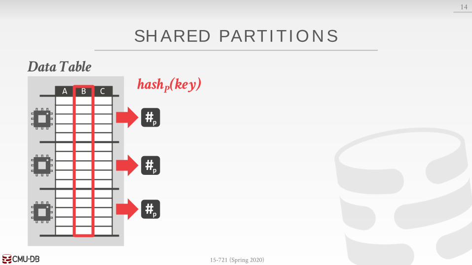
Approach #1: Shared Partitions→ Single global set of partitions that all threads update.→ Must use a latch to synchronize threads.
Approach #2: Private Partitions→ Each thread has its own set of partitions.→ Must consolidate them after all threads finish.
13
15-721 (Spring 2020)
SHARED PARTITIONS
14
Data Table
A B ChashP(key)
#p
#p
#p

15-721 (Spring 2020)
Partitions
SHARED PARTITIONS
14
Data Table
A B ChashP(key)
P1
⋮
P2
Pn
#p
#p
#p

15-721 (Spring 2020)
Partitions
PRIVATE PARTITIONS
15
Data Table
A B ChashP(key)
#p
#p
#p

15-721 (Spring 2020)
Partitions
PRIVATE PARTITIONS
15
Data Table
A B ChashP(key)
#p
#p
#p

15-721 (Spring 2020)
Partitions
PRIVATE PARTITIONS
15
Data Table
A B ChashP(key)
#p
#p
#p
Combined
P1
⋮
P2
Pn

15-721 (Spring 2020)
Partitions
PRIVATE PARTITIONS
15
Data Table
A B ChashP(key)
#p
#p
#p
Combined
P1
⋮
P2
Pn

15-721 (Spring 2020)
RADIX PARTITIONING
Scan the input relation multiple times to generate the partitions.
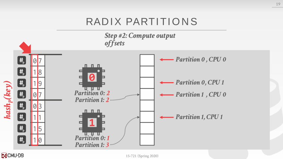
Multi-step pass over the relation:→ Step #1: Scan R and compute a histogram of the # of
tuples per hash key for the radix at some offset.→ Step #2: Use this histogram to determine output offsets
by computing the prefix sum.→ Step #3: Scan R again and partition them according to the
hash key.
16

15-721 (Spring 2020)
RADIX
The radix of a key is the value of an integer at a position (using its base).
17
89 12 23 08 41 64Keys

15-721 (Spring 2020)
RADIX
The radix of a key is the value of an integer at a position (using its base).
17
89 12 23 08 41 64
9 2 3 8 1 4
Keys
Radix

15-721 (Spring 2020)
RADIX
The radix of a key is the value of an integer at a position (using its base).
17
89 12 23 08 41 64Keys
Radix 8 1 2 0 4 6

15-721 (Spring 2020)
PREFIX SUM
The prefix sum of a sequence of numbers(x0, x1, …, xn)
is a second sequence of numbers(y0, y1, …, yn)
that is a running total of the input sequence.
18
+ + + + +
1 2 3 4 5 6
1 3 6 10 15 21
Input
Prefix Sum

15-721 (Spring 2020)
RADIX PARTITIONS
19
Step #1: Inspect input, create histograms
0 7
1 8
1 9
0 7
0 3
1 1
1 5
1 0
0
1
#p
#p
#p
#p
#p
#p
#p
#p
hash
P(k
ey)

15-721 (Spring 2020)
RADIX PARTITIONS
19
Step #1: Inspect input, create histograms
0 7
1 8
1 9
0 7
0 3
1 1
1 5
1 0
0
1
#p
#p
#p
#p
#p
#p
#p
#p
hash
P(k
ey)

15-721 (Spring 2020)
RADIX PARTITIONS
19
Step #1: Inspect input, create histograms
Partition 0: 2Partition 1: 2
Partition 0: 1Partition 1: 3
0 7
1 8
1 9
0 7
0 3
1 1
1 5
1 0
0
1
#p
#p
#p
#p
#p
#p
#p
#p
hash
P(k
ey)

15-721 (Spring 2020)
RADIX PARTITIONS
19
Partition 0: 2Partition 1: 2
Partition 0: 1Partition 1: 3
Partition 0
Partition 0, CPU 1
Partition 1
Partition 1, CPU 1
Step #2: Compute output offsets
, CPU 0
, CPU 0
0 7
1 8
1 9
0 7
0 3
1 1
1 5
1 0
0
1
#p
#p
#p
#p
#p
#p
#p
#p
hash
P(k
ey)
15-721 (Spring 2020)
RADIX PARTITIONS
19
Partition 0: 2Partition 1: 2
Partition 0: 1Partition 1: 3
Partition 0
Partition 0, CPU 1
Partition 1
Partition 1, CPU 1
Step #2: Compute output offsets
, CPU 0
, CPU 0
0 7
1 8
1 9
0 7
0 3
1 1
1 5
1 0
0
1
#p
#p
#p
#p
#p
#p
#p
#p
hash
P(k
ey)

15-721 (Spring 2020)
RADIX PARTITIONS
19
Partition 0: 2Partition 1: 2
Partition 0: 1Partition 1: 3
Partition 0
Partition 0, CPU 1
Partition 1
Partition 1, CPU 1
Step #3: Read inputand partition
0 7
0 3
, CPU 0
, CPU 0
0 7
1 8
1 9
0 7
0 3
1 1
1 5
1 0
0
1
#p
#p
#p
#p
#p
#p
#p
#p
hash
P(k
ey)

15-721 (Spring 2020)
RADIX PARTITIONS
19
Partition 0: 2Partition 1: 2
Partition 0: 1Partition 1: 3
Partition 0
Partition 0, CPU 1
Partition 1
Partition 1, CPU 1
Step #3: Read inputand partition
0 7
0 7
0 3
1 8
1 9
1 1
1 5
1 0
, CPU 0
, CPU 0
0 7
1 8
1 9
0 7
0 3
1 1
1 5
1 0
0
1
#p
#p
#p
#p
#p
#p
#p
#p
hash
P(k
ey)

15-721 (Spring 2020)
RADIX PARTITIONS
19
Partition 0: 2Partition 1: 2
Partition 0: 1Partition 1: 3
Partition 0
Partition 1
0 7
0 7
0 3
1 8
1 9
1 1
1 5
1 0
Recursively repeat until target number of partitions have been created
0 7
1 8
1 9
0 7
0 3
1 1
1 5
1 0
0
1
#p
#p
#p
#p
#p
#p
#p
#p
hash
P(k
ey)

15-721 (Spring 2020)
RADIX PARTITIONS
19
Partition 0: 2Partition 1: 2
Partition 0: 1Partition 1: 3
0 7
0 7
0 3
1 8
1 9
1 1
1 5
1 0
Recursively repeat until target number of partitions have been created
0 7
1 8
1 9
0 7
0 3
1 1
1 5
1 0
0
1
#p
#p
#p
#p
#p
#p
#p
#p
hash
P(k
ey)

15-721 (Spring 2020)
RADIX PARTITIONS
19
Partition 0: 2Partition 1: 2
Partition 0: 1Partition 1: 3
0 7
0 7
0 3
1 8
1 9
1 1
1 5
1 0
Recursively repeat until target number of partitions have been created
0 7
1 8
1 9
0 7
0 3
1 1
1 5
1 0
0
1
#p
#p
#p
#p
#p
#p
#p
#p
hash
P(k
ey)

15-721 (Spring 2020)
BUILD PHASE
The threads are then to scan either the tuples (or partitions) of R.
For each tuple, hash the join key attribute for that tuple and add it to the appropriate bucket in the hash table.→ The buckets should only be a few cache lines in size.
20

15-721 (Spring 2020)
HASH TABLE
Design Decision #1: Hash Function→ How to map a large key space into a smaller domain.→ Trade-off between being fast vs. collision rate.
Design Decision #2: Hashing Scheme→ How to handle key collisions after hashing.→ Trade-off between allocating a large hash table vs.
additional instructions to find/insert keys.
21
15-721 (Spring 2020)
HASH FUNCTIONS
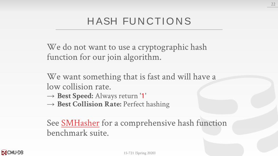
We do not want to use a cryptographic hash function for our join algorithm.
We want something that is fast and will have a low collision rate.→ Best Speed: Always return '1'→ Best Collision Rate: Perfect hashing
See SMHasher for a comprehensive hash function benchmark suite.
22
15-721 (Spring 2020)
HASH FUNCTIONS
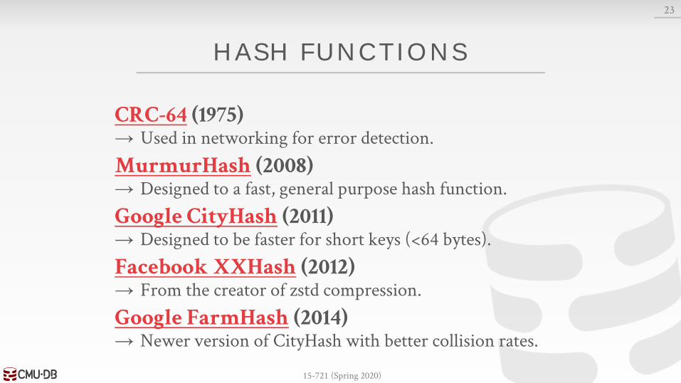
CRC-64 (1975)→ Used in networking for error detection.
MurmurHash (2008)→ Designed to a fast, general purpose hash function.
Google CityHash (2011)→ Designed to be faster for short keys (<64 bytes).
Facebook XXHash (2012)→ From the creator of zstd compression.
Google FarmHash (2014)→ Newer version of CityHash with better collision rates.
23
15-721 (Spring 2020)
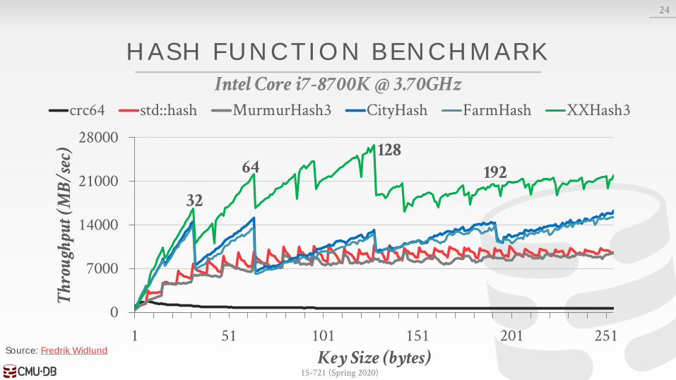
HASH FUNCTION BENCHMARK
24
0
7000
14000
21000
28000
1 51 101 151 201 251
Thr
ough
put (
MB
/sec
)
Key Size (bytes)
crc64 std::hash MurmurHash3 CityHash FarmHash XXHash3
Source: Fredrik Widlund
Intel Core i7-8700K @ 3.70GHz
32
64128
192

15-721 (Spring 2020)
HASHING SCHEMES
Approach #1: Chained Hashing
Approach #2: Linear Probe Hashing
Approach #3: Robin Hood Hashing
Approach #4: Hopscotch Hashing
Approach #5: Cuckoo Hashing
25

15-721 (Spring 2020)
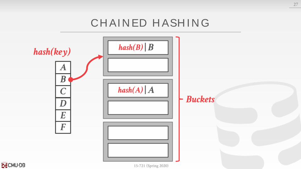
CHAINED HASHING
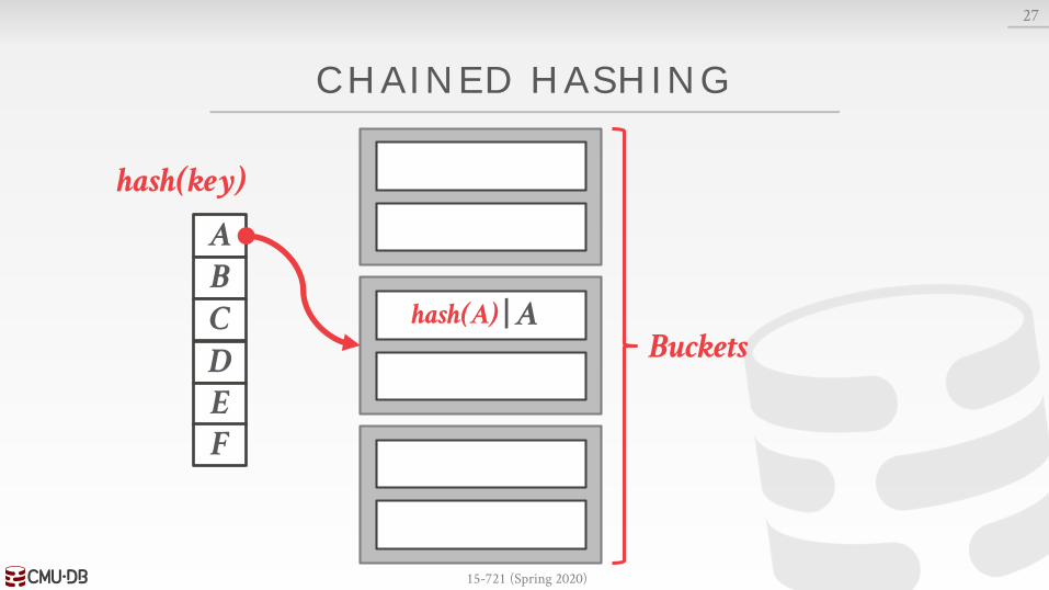
Maintain a linked list of buckets for each slot in the hash table.
Resolve collisions by placing all elements with the same hash key into the same bucket.→ To determine whether an element is present, hash to its
bucket and scan for it.→ Insertions and deletions are generalizations of lookups.
26

15-721 (Spring 2020)
CHAINED HASHING
27
ABCD
hash(key)
EF
15-721 (Spring 2020)
CHAINED HASHING
27
ABCD
hash(key)
EF
| Ahash(A)Buckets
15-721 (Spring 2020)
CHAINED HASHING
27
ABCD
hash(key)
EF
| Ahash(A)
| Bhash(B)
Buckets

15-721 (Spring 2020)
CHAINED HASHING
27
ABCD
hash(key)
EF
| Ahash(A)
| Bhash(B)
Buckets| Chash(C)

15-721 (Spring 2020)
CHAINED HASHING
27
ABCD
hash(key)
EF
| Ahash(A)
| Bhash(B)
Buckets| Chash(C)

15-721 (Spring 2020)
CHAINED HASHING
27
ABCD
hash(key)
EF
| Ahash(A)
| Bhash(B)
| Chash(C)
| Dhash(D)

15-721 (Spring 2020)
CHAINED HASHING
27
ABCD
hash(key)
EF
| Ahash(A)
| Bhash(B)
| Chash(C)
| Dhash(D)
| Ehash(E)

15-721 (Spring 2020)
CHAINED HASHING
27
ABCD
hash(key)
EF
| Ahash(A)
| Bhash(B)
| Chash(C)
| Dhash(D)
| Ehash(E)
| Fhash(F)
15-721 (Spring 2020)
CHAINED HASHING
27
ABCD
hash(key)
EF
| Ahash(A)
| Bhash(B)
| Chash(C)
| Dhash(D)
| Ehash(E)
| Fhash(F)
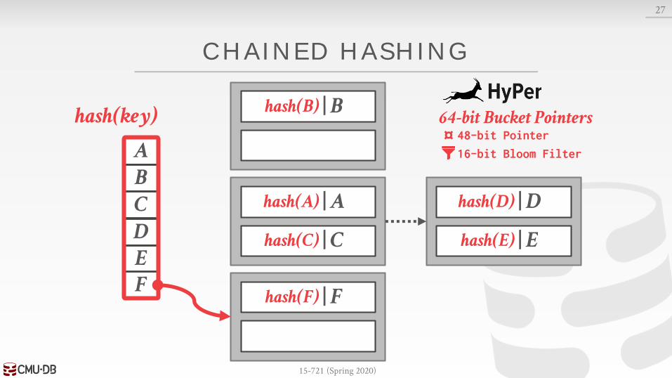
64-bit Bucket Pointers
16-bit Bloom Filter
48-bit Pointer¤

15-721 (Spring 2020)
LINEAR PROBE HASHING
Single giant table of slots.
Resolve collisions by linearly searching for the next free slot in the table.→ To determine whether an element is present, hash to a
location in the table and scan for it.→ Must store the key in the table to know when to stop
scanning.→ Insertions and deletions are generalizations of lookups.
28

15-721 (Spring 2020)
LINEAR PROBE HASHING
29
ABCD
hash(key)
| Ahash(A)
EF

15-721 (Spring 2020)
LINEAR PROBE HASHING
29
ABCD
hash(key)
| Ahash(A)
| Bhash(B)
EF

15-721 (Spring 2020)
LINEAR PROBE HASHING
29
ABCD
hash(key)
| Ahash(A)
| Bhash(B)
EF

15-721 (Spring 2020)
LINEAR PROBE HASHING
29
ABCD
hash(key)
| Ahash(A)
| Bhash(B)
| Chash(C)
EF

15-721 (Spring 2020)
LINEAR PROBE HASHING
29
ABCD
hash(key)
| Ahash(A)
| Bhash(B)
| Chash(C)
| Dhash(D)EF

15-721 (Spring 2020)
LINEAR PROBE HASHING
29
ABCD
hash(key)
| Ahash(A)
| Bhash(B)
| Chash(C)
| Dhash(D)EF

15-721 (Spring 2020)
LINEAR PROBE HASHING
29
ABCD
hash(key)
| Ahash(A)
| Bhash(B)
| Chash(C)
| Dhash(D)E
| Ehash(E)F

15-721 (Spring 2020)
LINEAR PROBE HASHING
29
ABCD
hash(key)
| Ahash(A)
| Bhash(B)
| Chash(C)
| Dhash(D)E
| Ehash(E)F
| Fhash(F)

15-721 (Spring 2020)
OBSERVATION
To reduce the # of wasteful comparisons during the join, it is important to avoid collisions of hashed keys.
This requires a chained hash table with ~2× the number of slots as the # of elements in R.
30
15-721 (Spring 2020)
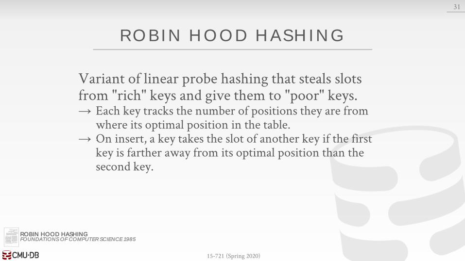
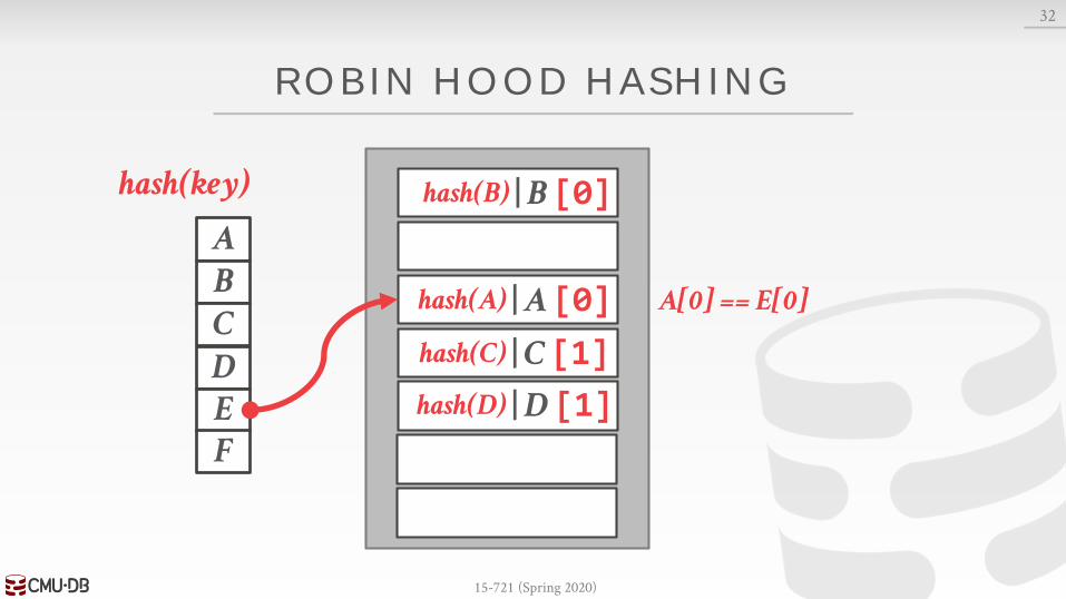
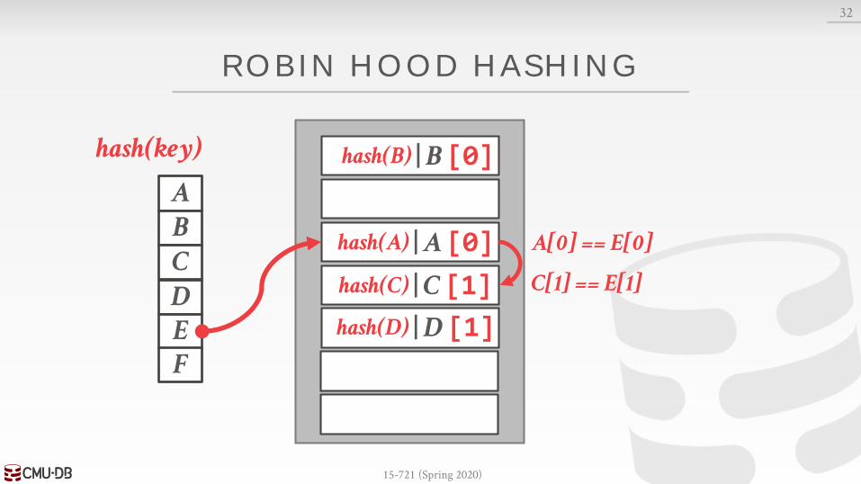
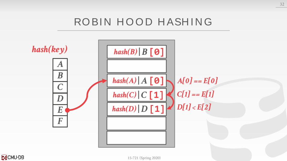
ROBIN HOOD HASHING
Variant of linear probe hashing that steals slots from "rich" keys and give them to "poor" keys.→ Each key tracks the number of positions they are from
where its optimal position in the table.→ On insert, a key takes the slot of another key if the first
key is farther away from its optimal position than the second key.
31
ROBIN HOOD HASHING FOUNDATIONS OF COMPUTER SCIENCE 1985

15-721 (Spring 2020)
ROBIN HOOD HASHING
32
ABCD
hash(key)
| A [0]hash(A)
E
# of "Jumps" From First Position
F

15-721 (Spring 2020)
ROBIN HOOD HASHING
32
ABCD
hash(key)
| A [0]hash(A)
| B [0]hash(B)
EF

15-721 (Spring 2020)
ROBIN HOOD HASHING
32
ABCD
hash(key)
| A [0]hash(A)
| B [0]hash(B)
EF
A[0] == C[0]

15-721 (Spring 2020)
ROBIN HOOD HASHING
32
ABCD
hash(key)
| A [0]hash(A)
| B [0]hash(B)
| C [1]hash(C)
EF
A[0] == C[0]

15-721 (Spring 2020)
ROBIN HOOD HASHING
32
ABCD
hash(key)
| A [0]hash(A)
| B [0]hash(B)
| C [1]hash(C)
EF
C[1] > D[0]

15-721 (Spring 2020)
ROBIN HOOD HASHING
32
ABCD
hash(key)
| A [0]hash(A)
| B [0]hash(B)
| C [1]hash(C)
| D [1]hash(D)EF
C[1] > D[0]
15-721 (Spring 2020)
ROBIN HOOD HASHING
32
ABCD
hash(key)
| A [0]hash(A)
| B [0]hash(B)
| C [1]hash(C)
| D [1]hash(D)E
A[0] == E[0]
F
15-721 (Spring 2020)
ROBIN HOOD HASHING
32
ABCD
hash(key)
| A [0]hash(A)
| B [0]hash(B)
| C [1]hash(C)
| D [1]hash(D)E
A[0] == E[0]
C[1] == E[1]
F
15-721 (Spring 2020)
ROBIN HOOD HASHING
32
ABCD
hash(key)
| A [0]hash(A)
| B [0]hash(B)
| C [1]hash(C)
| D [1]hash(D)E
A[0] == E[0]
C[1] == E[1]
D[1] < E[2]
F

15-721 (Spring 2020)
ROBIN HOOD HASHING
32
ABCD
hash(key)
| A [0]hash(A)
| B [0]hash(B)
| C [1]hash(C)
E | E [2]hash(E)
A[0] == E[0]
C[1] == E[1]
D[1] < E[2]
F | D [2]hash(D)

15-721 (Spring 2020)
ROBIN HOOD HASHING
32
ABCD
hash(key)
| A [0]hash(A)
| B [0]hash(B)
| C [1]hash(C)
E | E [2]hash(E)
F | D [2]hash(D)
| F [1]hash(F)
D[2] > F[0]

15-721 (Spring 2020)
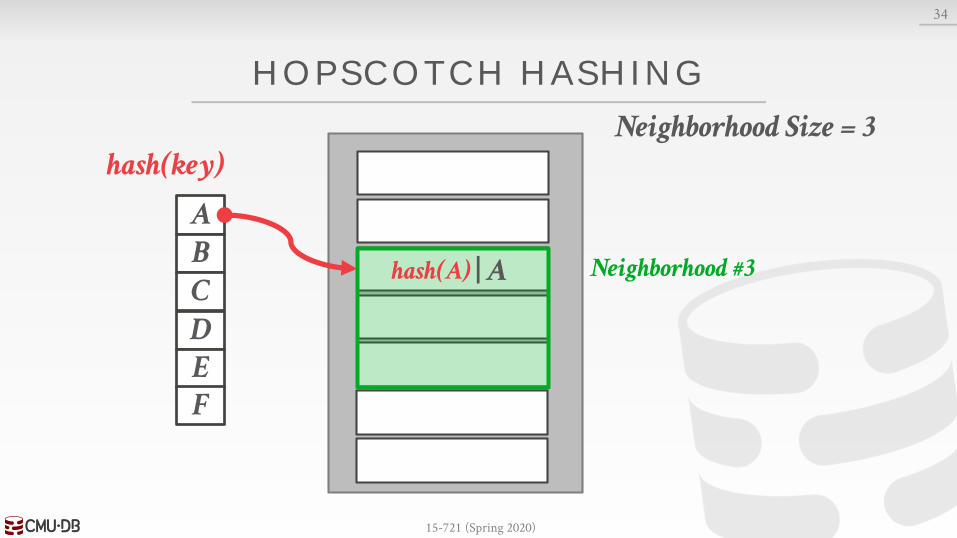
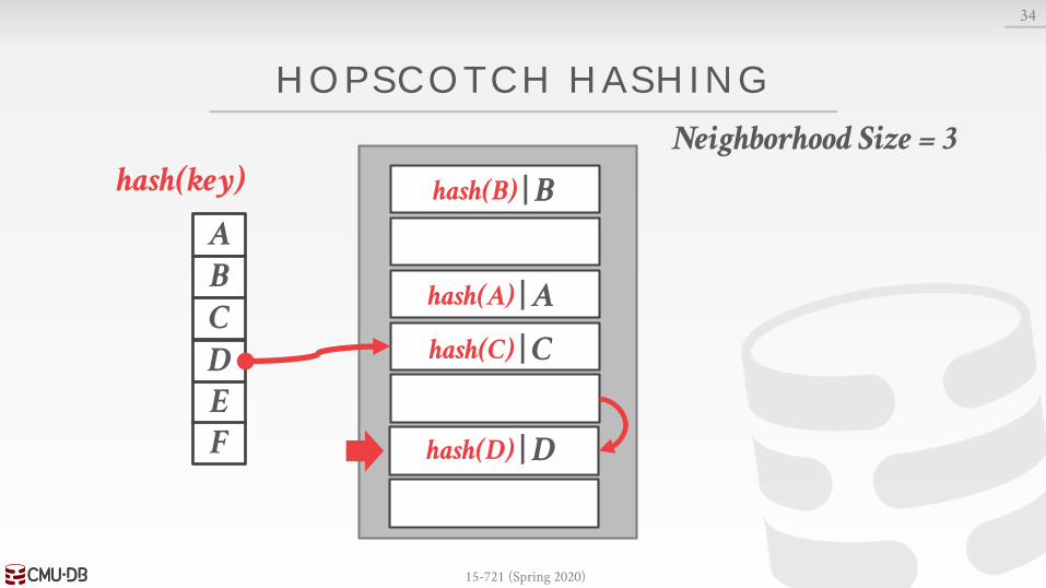
HOPSCOTCH HASHING
Variant of linear probe hashing where keys can move between positions in a neighborhood.→ A neighborhood is contiguous range of slots in the table.→ The size of a neighborhood is a configurable constant.
A key is guaranteed to be in its neighborhood or not exist in the table.
33
HOPSCOTCH HASHING SYMPOSIUM ON DISTRIBUTED COMPUTING 2008

15-721 (Spring 2020)
HOPSCOTCH HASHING
34
ABCD
hash(key)
EF
Neighborhood Size = 3

15-721 (Spring 2020)
HOPSCOTCH HASHING
34
ABCD
hash(key)
EF
Neighborhood Size = 3
Neighborhood #1

15-721 (Spring 2020)
HOPSCOTCH HASHING
34
ABCD
hash(key)
EF
Neighborhood Size = 3
Neighborhood #1
Neighborhood #2
Neighborhood #3
⋮

15-721 (Spring 2020)
HOPSCOTCH HASHING
34
ABCD
hash(key)
EF
Neighborhood Size = 3
Neighborhood #3
15-721 (Spring 2020)
HOPSCOTCH HASHING
34
ABCD
hash(key)
EF
Neighborhood Size = 3
Neighborhood #3| Ahash(A)

15-721 (Spring 2020)
HOPSCOTCH HASHING
34
ABCD
hash(key)
EF
Neighborhood Size = 3
Neighborhood #1
| Ahash(A)

15-721 (Spring 2020)
HOPSCOTCH HASHING
34
ABCD
hash(key)
EF
Neighborhood Size = 3
Neighborhood #1
| Ahash(A)
| Bhash(B)

15-721 (Spring 2020)
HOPSCOTCH HASHING
34
ABCD
hash(key)
EF
Neighborhood Size = 3
Neighborhood #3| Ahash(A)
| Bhash(B)

15-721 (Spring 2020)
HOPSCOTCH HASHING
34
ABCD
hash(key)
EF
Neighborhood Size = 3
Neighborhood #3| Ahash(A)
| Bhash(B)

15-721 (Spring 2020)
HOPSCOTCH HASHING
34
ABCD
hash(key)
EF
Neighborhood Size = 3
Neighborhood #3| Ahash(A)
| Bhash(B)
| Chash(C)

15-721 (Spring 2020)
HOPSCOTCH HASHING
34
ABCD
hash(key)
EF
Neighborhood Size = 3
| Ahash(A)
| Bhash(B)
| Chash(C)

15-721 (Spring 2020)
HOPSCOTCH HASHING
34
ABCD
hash(key)
EF
Neighborhood Size = 3
| Ahash(A)
| Bhash(B)
| Chash(C)

15-721 (Spring 2020)
HOPSCOTCH HASHING
34
ABCD
hash(key)
EF
Neighborhood Size = 3
| Ahash(A)
| Bhash(B)
| Chash(C)
| Dhash(D)

15-721 (Spring 2020)
HOPSCOTCH HASHING
34
ABCD
hash(key)
EF
Neighborhood Size = 3
| Ahash(A)
| Bhash(B)
| Chash(C)
| Dhash(D)

15-721 (Spring 2020)
HOPSCOTCH HASHING
34
ABCD
hash(key)
EF
Neighborhood Size = 3
Neighborhood #3| Ahash(A)
| Bhash(B)
| Chash(C)
| Dhash(D)

15-721 (Spring 2020)
HOPSCOTCH HASHING
34
ABCD
hash(key)
EF
Neighborhood Size = 3
Neighborhood #3| Ahash(A)
| Bhash(B)
| Chash(C)
| Dhash(D)

15-721 (Spring 2020)
HOPSCOTCH HASHING
34
ABCD
hash(key)
EF
Neighborhood Size = 3
Neighborhood #3| Ahash(A)
| Bhash(B)
| Chash(C)
| Dhash(D)
15-721 (Spring 2020)
HOPSCOTCH HASHING
34
ABCD
hash(key)
EF
Neighborhood Size = 3
| Ahash(A)
| Bhash(B)
| Chash(C)
| Dhash(D)

15-721 (Spring 2020)
HOPSCOTCH HASHING
34
ABCD
hash(key)
EF
Neighborhood Size = 3
Neighborhood #3| Ahash(A)
| Bhash(B)
| Chash(C)
| Dhash(D)
| Ehash(E)

15-721 (Spring 2020)
HOPSCOTCH HASHING
34
ABCD
hash(key)
EF
Neighborhood Size = 3
Neighborhood #6
| Ahash(A)
| Bhash(B)
| Chash(C)
| Dhash(D)
| Ehash(E)

15-721 (Spring 2020)
HOPSCOTCH HASHING
34
ABCD
hash(key)
EF
Neighborhood Size = 3
Neighborhood #6
| Ahash(A)
| Bhash(B)
| Chash(C)
| Dhash(D)
| Ehash(E)
| Fhash(F)

15-721 (Spring 2020)
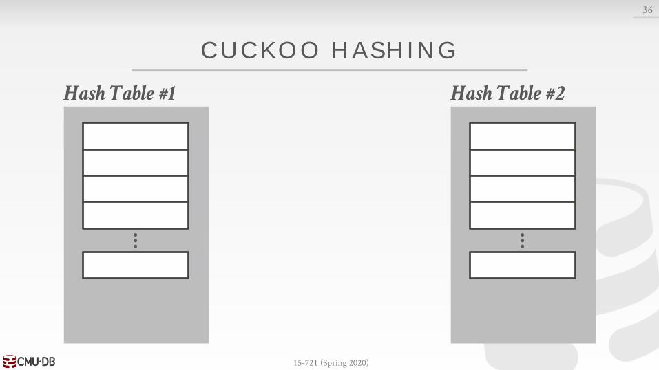
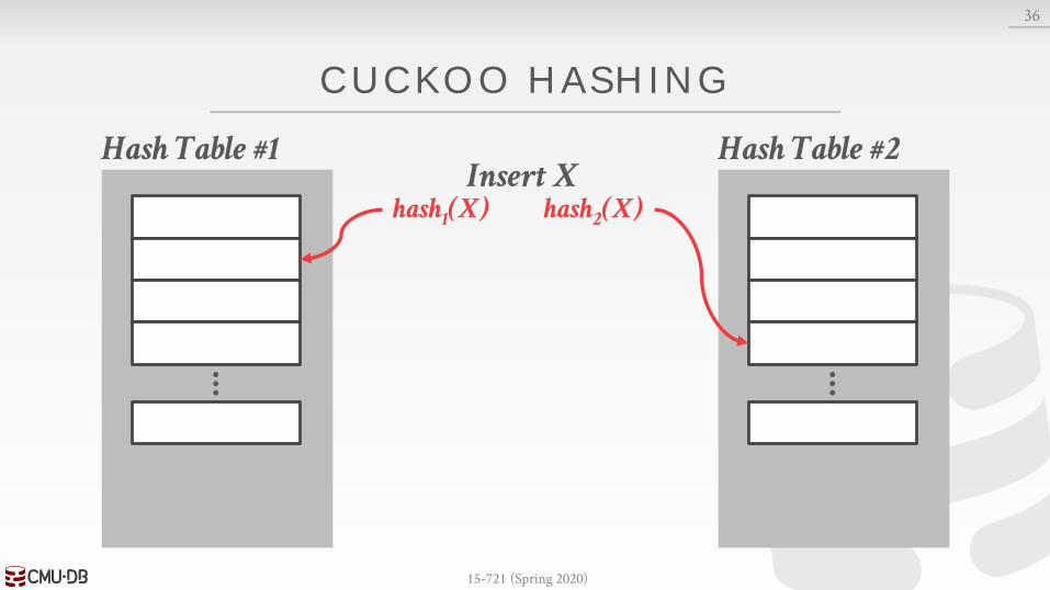
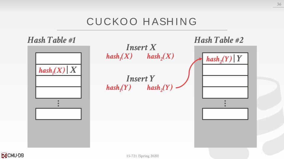
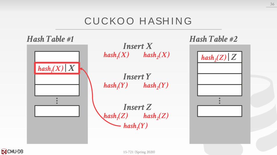
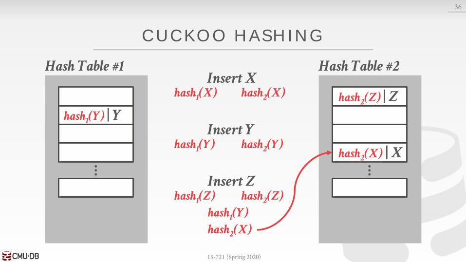
CUCKOO HASHING
Use multiple tables with different hash functions.→ On insert, check every table and pick anyone that has a
free slot.→ If no table has a free slot, evict the element from one of
them and then re-hash it find a new location.
Look-ups are always O(1) because only one location per hash table is checked.
35
15-721 (Spring 2020)
CUCKOO HASHING
36
Hash Table #1
⋮
Hash Table #2
⋮
15-721 (Spring 2020)
CUCKOO HASHING
36
Hash Table #1
⋮
Hash Table #2
⋮
Insert Xhash1(X) hash2(X)

15-721 (Spring 2020)
CUCKOO HASHING
36
Hash Table #1
⋮
Hash Table #2
⋮
Insert Xhash1(X) hash2(X)
hash1(X) | X

15-721 (Spring 2020)
CUCKOO HASHING
36
Hash Table #1
⋮
Hash Table #2
⋮
Insert Xhash1(X) hash2(X)
Insert Yhash1(Y) hash2(Y)
hash1(X) | X
15-721 (Spring 2020)
CUCKOO HASHING
36
Hash Table #1
⋮
Hash Table #2
⋮
Insert Xhash1(X) hash2(X)
Insert Yhash1(Y) hash2(Y)
hash1(X) | Xhash2(Y) | Y

15-721 (Spring 2020)
CUCKOO HASHING
36
Hash Table #1
⋮
Hash Table #2
⋮
Insert Xhash1(X) hash2(X)
Insert Yhash1(Y) hash2(Y)
hash1(X) | Xhash2(Y) | Y
Insert Zhash1(Z) hash2(Z)

15-721 (Spring 2020)
CUCKOO HASHING
36
Hash Table #1
⋮
Hash Table #2
⋮
Insert Xhash1(X) hash2(X)
Insert Yhash1(Y) hash2(Y)
hash1(X) | Xhash2(Y) | Y
Insert Zhash1(Z) hash2(Z)

15-721 (Spring 2020)
CUCKOO HASHING
36
Hash Table #1
⋮
Hash Table #2
⋮
Insert Xhash1(X) hash2(X)
Insert Yhash1(Y) hash2(Y)
hash1(X) | X
Insert Zhash1(Z) hash2(Z)
hash2(Z) | Z
hash1(Y)
15-721 (Spring 2020)
CUCKOO HASHING
36
Hash Table #1
⋮
Hash Table #2
⋮
Insert Xhash1(X) hash2(X)
Insert Yhash1(Y) hash2(Y)
hash1(X) | X
Insert Zhash1(Z) hash2(Z)
hash2(Z) | Z
hash1(Y)

15-721 (Spring 2020)
CUCKOO HASHING
36
Hash Table #1
⋮
Hash Table #2
⋮
Insert Xhash1(X) hash2(X)
Insert Yhash1(Y) hash2(Y)
Insert Zhash1(Z) hash2(Z)
hash2(Z) | Z
hash1(Y)
hash1(Y) | Y
15-721 (Spring 2020)
CUCKOO HASHING
36
Hash Table #1
⋮
Hash Table #2
⋮
Insert Xhash1(X) hash2(X)
Insert Yhash1(Y) hash2(Y)
Insert Zhash1(Z) hash2(Z)
hash2(Z) | Z
hash1(Y)
hash1(Y) | Y
hash2(X)
hash2(X) | X

15-721 (Spring 2020)
CUCKOO HASHING
Threads have to make sure that they don’t get stuck in an infinite loop when moving keys.
If we find a cycle, then we can rebuild the entire hash tables with new hash functions.→ With two hash functions, we (probably) won’t need to
rebuild the table until it is at about 50% full.→ With three hash functions, we (probably) won’t need to
rebuild the table until it is at about 90% full.
37

15-721 (Spring 2020)
PROBE PHASE
For each tuple in S, hash its join key and check to see whether there is a match for each tuple in corresponding bucket in the hash table constructed for R.→ If inputs were partitioned, then assign each thread a
unique partition.→ Otherwise, synchronize their access to the cursor on S.
38

15-721 (Spring 2020)
PROBE PHASE BLOOM FILTER
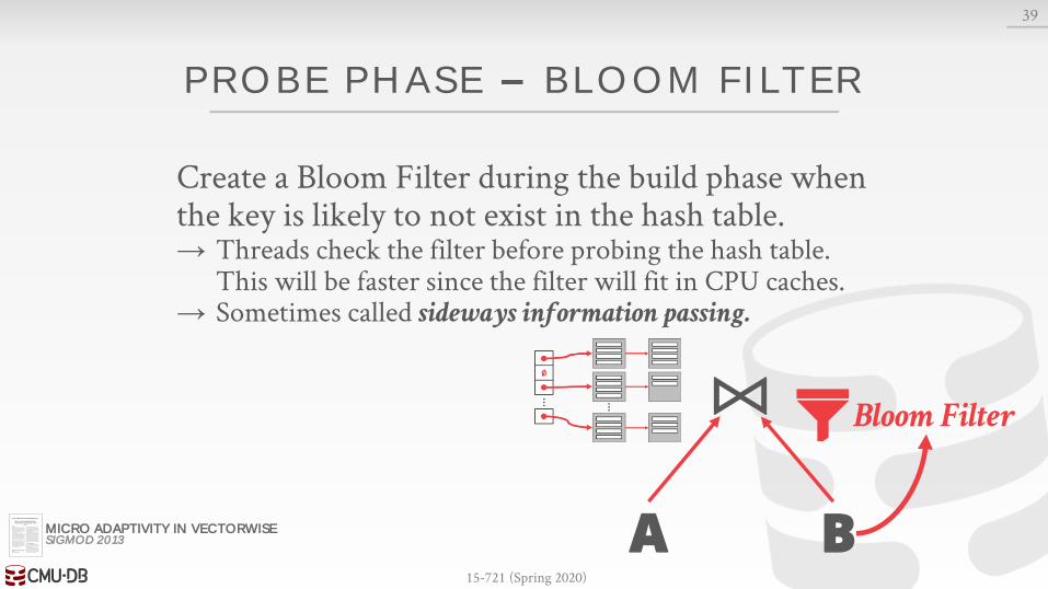
Create a Bloom Filter during the build phase when the key is likely to not exist in the hash table.→ Threads check the filter before probing the hash table.
This will be faster since the filter will fit in CPU caches.→ Sometimes called sideways information passing.
39
A B
⨝
MICRO ADAPTIVITY IN VECTORWISESIGMOD 2013

15-721 (Spring 2020)
PROBE PHASE BLOOM FILTER
Create a Bloom Filter during the build phase when the key is likely to not exist in the hash table.→ Threads check the filter before probing the hash table.
This will be faster since the filter will fit in CPU caches.→ Sometimes called sideways information passing.
39
A B
⨝Bloom Filter
MICRO ADAPTIVITY IN VECTORWISESIGMOD 2013
15-721 (Spring 2020)
PROBE PHASE BLOOM FILTER
Create a Bloom Filter during the build phase when the key is likely to not exist in the hash table.→ Threads check the filter before probing the hash table.
This will be faster since the filter will fit in CPU caches.→ Sometimes called sideways information passing.
39
A B
⨝ Bloom Filter
MICRO ADAPTIVITY IN VECTORWISESIGMOD 2013

15-721 (Spring 2020)
HASH JOIN VARIANTS
40
No-P Shared-P Private-P Radix
Partitioning No Yes Yes Yes
Input scans 0 1 1 2
Sync during partitioning
– Spinlock per tuple
Barrier, once at end
Barrier, 4 · #passes
Hash table Shared Private Private Private
Sync during build phase
Yes No No No
Sync during probe phase
No No No No

15-721 (Spring 2020)
BENCHMARKS
Primary key – foreign key join→ Outer Relation (Build): 16M tuples, 16 bytes each→ Inner Relation (Probe): 256M tuples, 16 bytes each
Uniform and highly skewed (Zipf; s=1.25)
No output materialization
41
DESIGN AND EVALUATION OF MAIN MEMORY HASH JOIN ALGORITHMS FOR MULTI-CORE CPUSSIGMOD 2011

15-721 (Spring 2020)
HASH JOIN UNIFORM DATA SET
42
0
40
80
120
160
No Partitioning Shared Partitioning
Private Partitioning
Radix
Cyc
les /
Ou
tpu
t Tu
ple
Partition Build Probe
Intel Xeon CPU X5650 @ 2.66GHz6 Cores with 2 Threads Per Core
60.2 67.676.8
47.3
24% faster thanNo Partitioning
3.3x cache misses70x TLB misses
Source: Spyros Blanas
15-721 (Spring 2020)
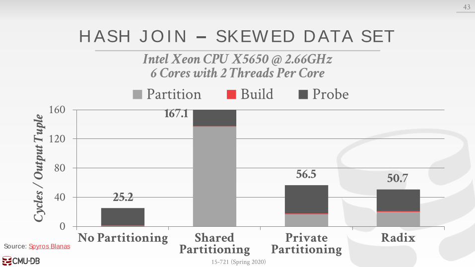
HASH JOIN SKEWED DATA SET
43
0
40
80
120
160
No Partitioning Shared Partitioning
Private Partitioning
Radix
Cyc
les /
Ou
tpu
t Tu
ple
Partition Build Probe
Intel Xeon CPU X5650 @ 2.66GHz6 Cores with 2 Threads Per Core
25.2
167.1
56.5 50.7
Source: Spyros Blanas

15-721 (Spring 2020)
OBSERVATION
We have ignored a lot of important parameters for all these algorithms so far.→ Whether to use partitioning or not?→ How many partitions to use?→ How many passes to take in partitioning phase?
In a real DBMS, the optimizer will select what it thinks are good values based on what it knows about the data (and maybe hardware).
44

15-721 (Spring 2020)
RADIX HASH JOIN UNIFORM DATA SET
45
0
40
80
120
64 256
512
1024
4096
8192
3276
8
1310
72 64 256
512
1024
4096
8192
3276
8
1310
72
Radix / 1-Pass Radix / 2-Pass
Cyc
les /
Ou
tpu
t Tu
ple
Partition Build Probe
Intel Xeon CPU X5650 @ 2.66GHzVarying the # of Partitions
▼No Partitioning+24% -5%
Source: Spyros Blanas

15-721 (Spring 2020)
RADIX HASH JOIN UNIFORM DATA SET
46
0
40
80
120
64 256
512
1024
4096
8192
3276
8
1310
72 64 256
512
1024
4096
8192
3276
8
1310
72
Radix / 1-Pass Radix / 2-Pass
Cyc
les /
Ou
tpu
t Tu
ple
Partition Build Probe
Intel Xeon CPU X5650 @ 2.66GHzVarying the # of Partitions
▼No Partitioning
Source: Spyros Blanas

15-721 (Spring 2020)
EFFECTS OF HYPER-THREADING
Radix join has fewer cache & TLB misses but this has marginal benefit.
Non-partitioned join relies on multi-threading for high performance.
47
Intel Xeon CPU X5650 @ 2.66GHzUniform Data Set
1
3
5
7
9
11
1 3 5 7 9 11
Spee
dup
Threads
No Partitioning Radix Ideal
Source: Spyros Blanas
Hyper-Threading

15-721 (Spring 2020)
TPC-H Q19
48
250 279301 285
0
100
200
300
400
No-Part (Linear)
No-Part (Array)
Radix (Linear)
Radix (Array)
Ru
nti
me
(ms)
Join Remaining Query
4× Intel Xeon CPU E7-4870v4Scale Factor 100
Source: Stefan Schuh

15-721 (Spring 2020)
PARTING THOUGHTS
Partitioned-based joins outperform no-partitioning algorithms is most settings, but it is non-trivial to tune it correctly.
AFAIK, every DBMS vendor picks one hash join implementation and does not try to be adaptive.
49

15-721 (Spring 2020)
NEXT CL ASS
Parallel Sort-Merge Joins
50