QuickTime™ and a decompressor

are needed to see this picture.

6.5 Part I: Partial Fractions

x + 2 +2

x−1

x +x+ 3x2 −1

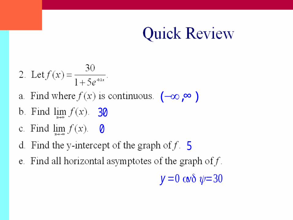
−∞,∞( )300

5

y =0 and y=30

2

5 3

2 3

xdx

x x

−− −∫ This would be a lot easier if we could

re-write it as two separate terms.

( )( )5 3

3 1

x

x x

−

− + 3 1

A B

x x= +

− +

1

→

These are called non-repeating linear factors.

You may already know a short-cut for this type of problem. We will get to that in a few minutes.

2

5 3

2 3

xdx

x x

−− −∫ This would be a lot easier if we could

re-write it as two separate terms.

( )( )5 3

3 1

x

x x

−

− + 3 1

A B

x x= +

− +Multiply by the common denominator.

( ) ( )5 3 1 3x A x B x− = + + −

5 3 3x Ax A Bx B− = + + − ⋅Set like-terms equal to each other.

5x Ax Bx= + 3 3A B− = − ⋅

5 A B= + 3 3A B− = −Solve two equations with two unknowns.

1

→

2

5 3

2 3

xdx

x x

−− −∫

( )( )5 3

3 1

x

x x

−

− + 3 1

A B

x x= +

− +

( ) ( )5 3 1 3x A x B x− = + + −

5 3 3x Ax A Bx B− = + + − ⋅

5x Ax Bx= + 3 3A B− = − ⋅

5 A B= + 3 3A B− = −Solve two equations with two unknowns.

5 A B= + 3 3A B− = −

3 3A B=− +

8 4B=

2 B= 5 2A= +

3 A=

3 2

3 1dx

x x+

− +∫

3ln 3 2ln 1x x C− + + +

This technique is calledPartial Fractions

1

→

2

5 3

2 3

xdx

x x

−− −∫ The short-cut for this type of problem is

called the Heaviside Method, after English engineer Oliver Heaviside.

( )( )5 3

3 1

x

x x

−

− + 3 1

A B

x x= +

− +Multiply by the common denominator.

( ) ( )5 3 1 3x A x B x− = + + −

8 0 4A B− = ⋅ + ⋅−

1

→

Let x = - 1

2 B=

( )12 4 0A B= ⋅ + ⋅ Let x = 3

3 A=

2

5 3

2 3

xdx

x x

−− −∫ The short-cut for this type of problem is

called the Heaviside Method, after English engineer Oliver Heaviside.

( )( )5 3

3 1

x

x x

−

− + 3 1

A B

x x= +

− +

( ) ( )5 3 1 3x A x B x− = + + −

8 0 4A B− = ⋅ + ⋅−

1

→

2 B=

( )12 4 0A B= ⋅ + ⋅3 A=

3 2

3 1dx

x x+

− +∫

3ln 3 2ln 1x x C− + + +

Ex:

2x +16x2 + x−6∫ dx =

= 2

x +8x2 + x−6∫ dx

= 2

A

x + 3∫ + B

x−2 dx A(x-2) + B(x+3) = x + 8

at x = 2, B = 2 and at x = -3, A = -1

= 2

−1x+ 3

+ 2

x−2 dx∫

⎡

⎣⎢

⎤

⎦⎥

= 2 −ln x+ 3 + 2ln x−2( ) + C

= 2 ln x −2( )

2

x+ 3 + C

Good News!

The AP Exam only requires non-repeating linear factors!

The more complicated methods of partial fractions are good to know, and you might see them in college, but they will not be on the AP exam or on my exam.

→

( )2

6 7

2

x

x

+

+

Repeated roots: we must use two terms for partial fractions.

( )22 2

A B

x x= +

+ +

( )6 7 2x A x B+ = + +

6 7 2x Ax A B+ = + +

6x Ax= 7 2A B= +

6 A= 7 2 6 B= ⋅ +

7 12 B= +

5 B− =

( )2

6 5

2 2x x−

+ +

2

→

3 2

2

2 4 3

2 3

x x x

x x

− − −− −

If the degree of the numerator is higher than the degree of the denominator, use long division first.

2 3 22 3 2 4 3x x x x x− − − − −2x

3 22 4 6x x x− −5 3x−

2

5 32

2 3

xxx x

−+

− −

( )( )5 3

23 1

xx

x x

−+

− + ( ) ( )3 2

23 1

xx x

= + +− +

4

(from example one)

→

Find

3x4 + 1

x2 - 1∫ dx

x2 - 1 3x4 + 1

3x4 - 3x2

3x2 + 1

3x2 - 3

3x2 + 3

4

Find

3x4 + 1

x2 - 1∫ dx

= 3x2 + 3 +

4

x2 - 1

⎛

⎝⎜⎞

⎠⎟∫ dx A(x+1) + B(x-1) = 4

= x3 + 3x +

2

x-1 +

-2

x+1

⎛

⎝⎜⎞

⎠⎟∫ dx

= x3 + 3x + 2 ln | x-1| - 2 ln | x+1| + C

at x = 1, A = 2; at x = -1, B = -2

( )( )22

2 4

1 1

x

x x

− +

+ −

irreduciblequadratic

factor

repeated root

( )22 1 1 1

Ax B C D

x x x

+= + +

+ − −

first degree numerator

( )( ) ( )( ) ( )2 2 22 4 1 1 1 1x Ax B x C x x D x− + = + − + + − + +

( )( ) ( )2 3 2 22 4 2 1 1x Ax B x x C x x x Dx D− + = + − + + − + − + +

3 2 2 3 2 22 4 2 2x Ax Ax Ax Bx Bx B Cx Cx Cx C Dx D− + = − + + − + + − + − + +

A challenging example:

→

3 2 2 3 2 22 4 2 2x Ax Ax Ax Bx Bx B Cx Cx Cx C Dx D− + = − + + − + + − + − + +

0 A C= + 0 2A B C D=− + − + 2 2A B C− = − + 4 B C D= − +

1 0 1 0 0

2 1 1 1 0

1 2 1 0 2

0 1 1 1 4

− −− −

−

2 r 3+ ⋅

r 1−

1 0 1 0 0

0 3 1 1 4

0 2 0 0 2

0 1 1 1 4

− −− −

−

( ) 2÷ −

1 0 1 0 0

0 1 0 0 1

0 3 1 1 4

0 1 1 1 4

− −−

3 r 2+ ⋅

r 2−

1 0 1 0 0

0 1 0 0 1

0 0 1 1 1

0 0 1 1 3

−− r 3+

→

1 0 1 0 0

0 1 0 0 1

0 3 1 1 4

0 1 1 1 4

− −−

3 r 2+ ⋅

r 2−

1 0 1 0 0

0 1 0 0 1

0 0 1 1 1

0 0 1 1 3

−− r 3+

1 0 1 0 0

0 1 0 0 1

0 0 1 1 1

0 0 0 2 2

− 2÷

1 0 1 0 0

0 1 0 0 1

0 0 1 1 1

0 0 0 1 1

− r 4−

1 0 1 0 0

0 1 0 0 1

0 0 1 0 2

0 0 0 1 1

−

r 3−

1 0 0 0 2

0 1 0 0 1

0 0 1 0 2

0 0 0 1 1

−

→

1 0 0 0 2

0 1 0 0 1

0 0 1 0 2

0 0 0 1 1

−

( )( )22

2 4

1 1

x

x x

− +

+ − ( )22 1 1 1

Ax B C D

x x x

+= + +

+ − −

( )22

2 1 2 1

1 1 1

x

x x x

+= − +

+ − −

We can do this problem on the TI-89:

( ) ( )22

2 4expand

1 1

x

x x

⎛ ⎞− ⋅ +⎜ ⎟⎜ ⎟+ ⋅ −⎝ ⎠

expand ((-2x+4)/((x^2+1)*(x-1)^2))

( )22 2

2 1 2 1

1 1 1 1

x

x x x x

⋅+ − +

+ + − −Of course with the TI-89, we could just integrate and wouldn’t need partial fractions!

3F2

6.5 Part II Logistic Growth

Greg Kelly, Hanford High School, Richland, WashingtonPhoto by Vickie Kelly, 2004

Columbian Ground SquirrelGlacier National Park, Montana

We have used the exponential growth equationto represent population growth.

0kty y e=

The exponential growth equation occurs when the rate of growth is proportional to the amount present.

If we use P to represent the population, the differential equation becomes: dP

kPdt

=

The constant k is called the relative growth rate.

/dP dtk

P=

→

The population growth model becomes: 0ktP P e=

However, real-life populations do not increase forever. There is some limiting factor such as food, living space or waste disposal.

There is a maximum population, or carrying capacity, M.

A more realistic model is the logistic growth model where

growth rate is proportional to both the amount present (P)

and the carrying capacity that remains: (M-P)

→

The equation then becomes:

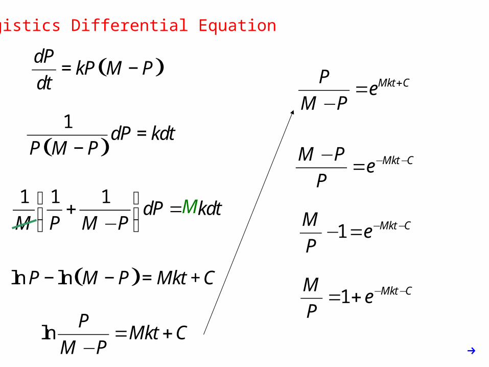
Logistics Differential Equation

( )dPkP M P

dt= −

We can solve this differential equation to find the logistics growth model.

→

PartialFractions

Logistics Differential Equation

( )dPkP M P

dt= −

( )1

dP kdtP M P

=−

( )1 A B

P M P P M P= +

− −

( )1 A M P BP= − +

1 AM AP BP= − +

1 AM=

1A

M=

0 AP BP=− +AP BP=A B=1

BM

=

1 1 1 dP kdt

M P M P⎛ ⎞+ =⎜ ⎟−⎝ ⎠

( )ln lnP M P Mkt C− − = +

lnP

Mkt CM P

= +− →

M

Logistics Differential Equation

Mkt CPe

M P+=

−

Mkt CM Pe

P− −−

=

1 Mkt CMe

P− −− =

1 Mkt CMe

P− −= +

→

( )dPkP M P

dt= −

( )1

dP kdtP M P

=−

1 1 1 dP kdt

M P M P⎛ ⎞+ =⎜ ⎟−⎝ ⎠

( )ln lnP M P Mkt C− − = +

lnP

Mkt CM P

= +−

M

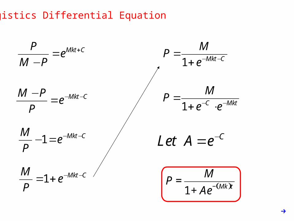
Logistics Differential Equation

1 Mkt C

MP

e− −=+

1 C Mkt

MP

e e− −=+ ⋅

CLet A e−=

( )1 Mk t

MP

Ae−=

+

→

Mkt CPe

M P+=

−

Mkt CM Pe

P− −−

=

1 Mkt CMe

P− −− =

1 Mkt CMe

P− −= +

Logistics Growth Model

( )1 Mk t

MP

Ae−=

+

→

Example:

Logistic Growth Model

Ten grizzly bears were introduced to a national park 10 years ago. There are 23 bears in the park at the present time. The park can support a maximum of 100 bears.

Assuming a logistic growth model, when will the bear population reach 50? 75? 100?

→

Ten grizzly bears were introduced to a national park 10 years ago. There are 23 bears in the park at the present time. The park can support a maximum of 100 bears.

Assuming a logistic growth model, when will the bear population reach 50? 75? 100?

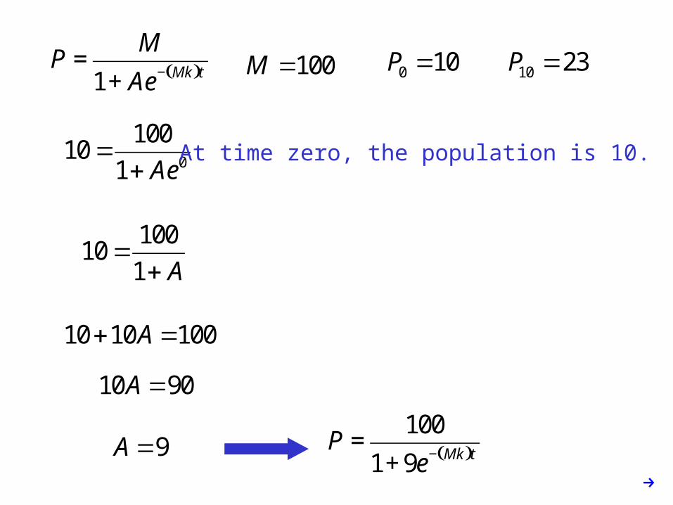
( )1 Mk t

MP

Ae−=

+100M = 0 10P = 10 23P =

→

( )1 Mk t

MP

Ae−=

+100M = 0 10P = 10 23P =

0

10010

1 Ae=

+

10010

1 A=

+

10 10 100A+ =

10 90A=

9A=

At time zero, the population is 10.

( )100

1 9 Mk tP

e−=

+→

100M = 0 10P = 10 23P =

After 10 years, the population is 23.

( )100

1 9 Mk tP

e−=

+

( )100 10

10023

1 9 ke− ⋅=

+

1000 1001 9

23ke−+ =

1000 779

23ke− =

1000 0.371981ke− =

1000 0.988913k− =−

0.00098891k =

0.1

100

1 9 tP

e−=

+→

( )1 Mk t

MP

Ae−=

+

0.1

100

1 9 tP

e−=

+

0

20

40

60

80

100

20 40 60 80 100Years

BearsWe can graph this equation and use “trace” to find the solutions.

y=50 at 22 years

y=75 at 33 years

y=100 at 75 years

Gorilla Population A certain wild animal preserve can support no more than

250 lowland gorillas. Twenty-eight gorillas were known to be in the preserve in 1970. Assume that the rate of growth of the population is

Where time t is in years.

a) Find a formula for the gorilla population in terms of t.

b) How long will it take the gorilla population to reach the carrying capacity of the preserve?

dP

dt = 0.0004 P (250 - P)

dP

dt = 0.0004 P (250 - P)

dP

P(250−P) = .0004 dt

A

P∫ + B

250−P dp = .0004 dt A 250−P( )∫ + B P( ) = 1

at P = 0, A = .004; at P = 250, B = .004

.004

P∫ + .004

250−P dp = .0004 dt∫

.004 ln P - ln 250−P( ) = .0004t +C

ln P - ln 250−P = .1t + C

.004 ln P - ln 250−P( ) = .0004t +C

ln

250−PP

= -.1t - C

250

P - 1 = C e−.1t

250

P = 1 + C e−.1t at (0,28), C = 7.92857

Note: 7.92857 = M

P0

- 1

and k = .0004 * M = .1

P

250 =

1

1 + 7.92857 e−.1t

P =

250

1 + 7.92857 e−.1t

250

P = 1 + C e−.1t at (0,28), C = 7.92857

Gorilla Population

dP

dt = 0.0004 P (250 - P)

P(t) ≈

2501 + 7.9286e- 0.1 t

A certain wild animal preserve can support no more than 250 lowland gorillas. Twenty-eight gorillas were known to be in the preserve in 1970. Assume that the rate of growth of the population is

Where time t is in years.

a) Find a formula for the gorilla population in terms of t.

b) How long will it take the gorilla population to reach the carrying capacity of the preserve?

83 years to reach 249.5 ≈250