6.3 continuous wavelet transforms · scalogram of this signal using a mexican hat wavelet of width...

i

i

i

i

i

i

i

i

180 6. Beyond wavelets

(a) (b)

FIGURE 6.2(a) 2-level Daub 9/7 wavelet transform of Barbara image with magnitudes offluctuation values larger than 8 shown in white. (b) Similar display for the2-level Daub 9/7 wavelet packet transform of Barbara image.

exhibits a more compact distribution of significant coefficients, hence a greatercompression, than the 4-level wavelet transform.

6.2.1 Fingerprint compression

This example also gives us some further insight into the WSQ method offingerprint compression. WSQ achieves at least 15:1 compression, withoutnoticeable loss of detail, on all fingerprint images. It achieves such a re-markable result by applying a wavelet packet transform for which not everysubimage is subjected to a further 1-level wavelet transform, but a large per-centage of subimages are further transformed. To illustrate why this mightbe advantageous, consider the two transforms of the Barbara image in Fig-ure 6.2. Notice that the vertical fluctuation v1 in the lower right quadrantof Figure 6.2(a) does not seem to be significantly compressed by applyinganother 1-level wavelet transform. Therefore, some advantage in compres-sion might be obtained by not applying a 1-level wavelet transform to thissubimage, while applying it to the other subimages. The wavelet packet trans-form used by WSQ is described in [6] and [7]. It should also be noted thatJPEG 2000 Part 2 allows for wavelet packet transforms, see p. 606 of [7].

6.3 Continuous wavelet transforms

In this section and the next we shall describe the concept of a continuous

wavelet transform (CWT), and how it can be approximated in a discrete formusing a computer. We begin our discussion by describing one type of CWT,known as the Mexican hat CWT, which has been used extensively in seismicanalysis. In the next section we turn to a second type of CWT, the GaborCWT, which has many applications to analyzing audio signals. Although wedo not have space for a thorough treatment of CWTs, we can nevertheless

i

i

i

i

i

i

i

i

6.3 Continuous wavelet transforms 181

introduce some of the essential ideas.The notion of a CWT is founded upon many of the concepts that we intro-

duced in our discussion of discrete wavelet analysis in Chapters 2 through 5,especially the ideas connected with discrete correlations and frequency analy-sis. A CWT provides a very redundant, but also very finely detailed, descrip-tion of a signal in terms of both time and frequency. CWTs are particularlyhelpful in tackling problems involving signal identification and detection ofhidden transients (hard to detect, short-lived elements of a signal).

To define a CWT we begin with a given function Ψ(x), which is called theanalyzing wavelet. For instance, if we define Ψ(x) by

Ψ(x) = 2πw−1/2[

1 − 2π(x/w)2]

e−π(x/w)2 , w = 1/16, (6.7)

then this analyzing wavelet is called a Mexican hat wavelet, with width pa-

rameter w = 1/16. See Figure 6.3(a).It is possible to choose other values for w besides 1/16, but this one ex-

ample should suffice. By graphing the Mexican hat wavelet using differentvalues of w, it is easy to see why w is called a width parameter. The smallerthe value of w, the more the energy of Ψ(x) is confined to a smaller intervalof the x-axis.

The Mexican hat wavelet is not the only kind of analyzing wavelet. In thenext section, we shall consider the Gabor wavelet, which is very advantageousfor analyzing recordings of speech or music. We begin in this section with theMexican hat wavelet because it allows us to more easily explain the conceptof a CWT.

Given an analyzing wavelet Ψ(x), a CWT of a discrete signal f is definedby computing several correlations of this signal with discrete samplings of thefunctions Ψs(x) defined by

Ψs(x) =1√s

Ψ(x

s

)

, s > 0. (6.8)

The parameter s is called a scale parameter. If we sample each signal Ψs(x) atdiscrete time values t1, t2, . . . , tN , where N is the length of f , then we generatethe discrete signals gs defined by

gs = ( Ψs(t1),Ψs(t2), . . . ,Ψs(tN ) ) .

A CWT of f then consists of a collection of discrete correlations (f : gs) overa finite collection of values of s. A common choice for these values is

s = 2−k/M , k = 0, 1, 2, . . . , I · M

where the positive integer I is called the number of octaves and the positiveinteger M is called the number of voices per octave. For example, 8 octavesand 16 voices per octave is the default choice in FAWAV. Another popularchoice is 6 octaves and 12 voices per octave. This latter choice of scales

i

i

i

i

i

i

i

i


0

(a) (b)

FIGURE 6.3(a) The Mexican hat wavelet, w = 1/16. (b) DFTs of discrete samplings of thiswavelet for scales s = 2−k/6, from k = 0 at the top, then k = 2, then k = 4, thenk = 6, down to k = 8 at the bottom.

corresponds—based on the relationship between scales and frequencies thatwe describe below—to the scale of notes on a piano (also known as the well-

tempered scale).The purpose of computing all these correlations is that a very finely de-

tailed time-frequency analysis of a signal can be carried out by making ajudicious choice of the width parameter w and the number of octaves andvoices. To see this, we observe that Formula (5.40) tells us that the DFTs ofthe correlations (f : gs) satisfy

(f : gs)F7−→ Ff Fgs. (6.9)

For a Mexican hat wavelet, Fgs is real-valued; hence Fgs = Fgs. ThereforeEquation (6.9) becomes

(f : gs)F7−→ Ff Fgs. (6.10)

Formula (6.10) is the basis for a very finely detailed time-frequency decompo-sition of a discrete signal f . For example, in Figure 6.3(b) we show graphs ofthe DFTs Fgs for the scale values s = 2−k/6, with k = 0, 2, 4, 6, and 8. Thesegraphs show that when these DFTs are multiplied with the DFT of f , theyprovide a decomposition of Ff into a succession of frequency bands. Thesesuccessive bands overlap each other, thus providing a very redundant decom-position of the DFT of f . Notice that the bands containing higher frequenciescorrespond to smaller scale values; there is a reciprocal relationship between

scale values and frequency values. It is also important to note that there is adecomposition in time, due to the essentially finite width of the Mexican hatwavelet [see Figure 6.3(a)].

A couple of examples should help to clarify these points. The first examplewe shall consider is a test case designed to illustrate the connection between

i

i

i

i

i

i

i

i

6.3 Continuous wavelet transforms 183

a CWT and the time-location of frequencies in a signal. The second exampleis an illustration of how a CWT can be used for analyzing an ECG signal.

For our first example, we shall analyze a discrete signal f , obtained from2048 equally spaced samples of the following analog signal:

sin(40πx)e−100π(x−.2)2

+ [sin(40πx) + 2 cos(160πx)] e−50π(x−.5)2

+ 2 sin(160πx)e−100π(x−.8)2 (6.11)

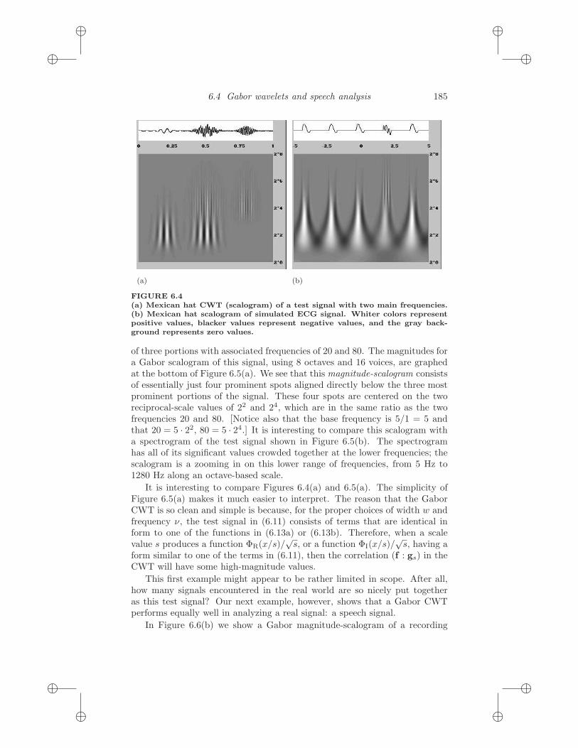
over the interval 0 ≤ x ≤ 1. See the top of Figure 6.4(a).The signal in (6.11) consists of three terms. The first term contains a sine

factor, sin(40πx), of frequency 20. Its other factor, e−100π(x−.2)2 , serves as adamping factor which limits the energy of this term to a small interval centeredon x = 0.2. This first term appears most prominently on the left-third of thegraph at the top of Figure 6.4(a). Likewise, the third term contains a sinefactor, 2 sin(160πx), of frequency 80, and this term appears most prominentlyon the right-third of the signal’s graph. Notice that this frequency of 80 isfour times as large as the first frequency of 20. Finally, the middle term

[sin(40πx) + 2 cos(160πx)] e−50π(x−.5)2

has a factor containing both of these two frequencies, and can be observedmost prominently within the middle of the signal’s graph.

The CWT, also known as a scalogram, for this signal is shown at thebottom of Figure 6.4(a). The analyzing wavelet used to produce this CWTwas a Mexican hat wavelet of width 1/16, with scales ranging over 8 octavesand 16 voices. The labels on the right side of the figure indicate reciprocals

of the scales used. Because of the reciprocal relationship between scale andfrequency noted above, this reciprocal-scale axis can also be viewed as a fre-quency axis. Notice that the four most prominent portions of this scalogramare aligned directly below the three most prominent parts of the signal. Ofequal importance is the fact that these four portions of the scalogram arecentered on two reciprocal-scales, 1/s ≈ 22.2 and 1/s ≈ 24.2. The secondreciprocal scale is four times larger than the first reciprocal scale, just as thefrequency 80 is four times larger than the frequency 20. Bearing this fact inmind, and recalling the alignment of the prominent regions of the scalogramwith the three parts of the signal, we can see that the CWT provides us witha time-frequency portrait of the signal.

We have shown that it is possible to correctly interpret the meaning ofthis scalogram; nevertheless, we can produce a much simpler and more easilyinterpretable scalogram for this test signal using a Gabor analyzing wavelet.See Figure 6.5(a). We shall discuss this Gabor scalogram in the next section.

Our second example uses a Mexican hat CWT for analyzing a signal con-taining several transient bursts, a simulated ECG signal first considered inSection 5.4. See the top of Figure 6.4(b). The bottom of Figure 6.4(b) is a

i

i

i

i

i

i

i

i


scalogram of this signal using a Mexican hat wavelet of width 2, over a rangeof 8 octaves and 16 voices. This scalogram shows how a Mexican hat waveletcan be used for detecting the onset and demise of each heartbeat. In particu-lar, the aberrant, fourth heartbeat is singled out from the others by the longervertical ridges extending upwards to the highest frequencies (at the eighth oc-tave). Although this example is only a simulation, it does show the ease withwhich the Mexican hat CWT detects the presence of short-lived parts of asignal. Similar identifications of transient bursts are needed in seismology forthe detection of earthquake tremors. Consequently, Mexican hat wavelets arewidely used in seismology.

6.4 Gabor wavelets and speech analysis

In this section we describe Gabor wavelets, which are similar to the Mexicanhat wavelets examined in the previous section, but provide a more powerfultool for analyzing speech and music. We shall first go over their definition,and then illustrate their use with some examples.

A Gabor wavelet, with width parameter w and frequency parameter ν, isthe following analyzing wavelet:

Ψ(x) = w−1/2e−π(x/w)2 ei2πνx/w. (6.12)

This wavelet is complex valued. Its real part ΨR(x) and imaginary part ΨI(x)are

ΨR(x) = w−1/2e−π(x/w)2 cos(2πνx/w), (6.13a)

ΨI(x) = w−1/2e−π(x/w)2 sin(2πνx/w). (6.13b)

The width parameter w plays the same role as for the Mexican hat wavelet;it controls the width of the region over which most of the energy of Ψ(x) isconcentrated. The value ν/w is called the base frequency for a Gabor CWT.

One advantage that Gabor wavelets have when analyzing sound signalsis that they contain factors of cosines and sines, as shown in (6.13a) and(6.13b). These cosine and sine factors allow the Gabor wavelets to createeasily interpretable scalograms of those signals which are combinations ofcosines and sines—the most common instances of such signals are recordedmusic and speech. We shall see this in a moment, but first we need to say alittle more about the CWT defined by a Gabor analyzing wavelet.

Because a Gabor wavelet is complex valued, it produces a complex-valuedCWT. For many signals, it is often sufficient to just examine the magnitudesof the Gabor CWT values. In particular, this is the case with the signalsanalyzed in the following examples.

For our first example, we use a Gabor wavelet with width 1 and frequency5 for analyzing the signal in (6.11). The graph of this signal is shown at the topof Figure 6.5(a). As we discussed in the previous section, this signal consists

i

i

i

i

i

i

i

i

6.4 Gabor wavelets and speech analysis 185

(a) (b)

FIGURE 6.4(a) Mexican hat CWT (scalogram) of a test signal with two main frequencies.(b) Mexican hat scalogram of simulated ECG signal. Whiter colors representpositive values, blacker values represent negative values, and the gray back-ground represents zero values.

of three portions with associated frequencies of 20 and 80. The magnitudes fora Gabor scalogram of this signal, using 8 octaves and 16 voices, are graphedat the bottom of Figure 6.5(a). We see that this magnitude-scalogram consistsof essentially just four prominent spots aligned directly below the three mostprominent portions of the signal. These four spots are centered on the tworeciprocal-scale values of 22 and 24, which are in the same ratio as the twofrequencies 20 and 80. [Notice also that the base frequency is 5/1 = 5 andthat 20 = 5 · 22, 80 = 5 · 24.] It is interesting to compare this scalogram witha spectrogram of the test signal shown in Figure 6.5(b). The spectrogramhas all of its significant values crowded together at the lower frequencies; thescalogram is a zooming in on this lower range of frequencies, from 5 Hz to1280 Hz along an octave-based scale.

It is interesting to compare Figures 6.4(a) and 6.5(a). The simplicity ofFigure 6.5(a) makes it much easier to interpret. The reason that the GaborCWT is so clean and simple is because, for the proper choices of width w andfrequency ν, the test signal in (6.11) consists of terms that are identical inform to one of the functions in (6.13a) or (6.13b). Therefore, when a scalevalue s produces a function ΦR(x/s)/

√s, or a function ΦI(x/s)/

√s, having a

form similar to one of the terms in (6.11), then the correlation (f : gs) in theCWT will have some high-magnitude values.

This first example might appear to be rather limited in scope. After all,how many signals encountered in the real world are so nicely put togetheras this test signal? Our next example, however, shows that a Gabor CWTperforms equally well in analyzing a real signal: a speech signal.

In Figure 6.6(b) we show a Gabor magnitude-scalogram of a recording

i

i

i

i

i

i

i

i


(a) (b)

FIGURE 6.5(a) Magnitudes of Gabor scalogram of test signal. (b) Spectrogram of testsignal. Darker regions denote larger magnitudes; lighter regions denote smallermagnitudes.

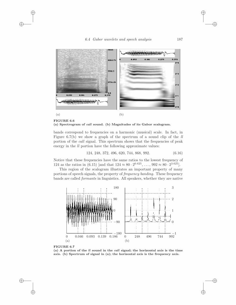
of the author saying the word call. The recorded signal, which is shown atthe top of the figure, consist of three main portions. The first two portionscorrespond to the two sounds, ca and ll, that form the word call. The ca

portion occupies a narrow area on the far left side of the call signal’s graph,while the ll portion occupies a much larger area consisting of the middlehalf of the call signal’s graph. The third portion lies at the right end of thesignal and is a “clipping sound” that is the start of the consonant “b” thatbegins the word “back” (the call signal was clipped from a recording of theauthor speaking the phrase “you call back”). For comparison, we have alsoplotted the call signal’s spectrogram in Figure 6.6(a). Again, as with our testsignal, the scalogram is able to zoom in and better display the time-frequencystructure of this speech signal.

To analyze the call signal, we used a Gabor wavelet of width 1/8 andfrequency 10 (hence a base frequency of 10/(1/8) = 80 Hz), with scales rangingover 4 octaves and 16 voices. The resulting magnitude-scalogram is composedof several regions. The largest region is a collection of several horizontal bandslying below the ll portion. We shall concentrate on analyzing this region.

This region below the ll portion consists of seven horizontal bands centeredon the following approximate reciprocal-scale values:

20.625, 21.625, 22.188, 22.625, 22.953, 22.97, 23.219, 23.625. (6.14)

If we divide each of these values by the smallest one, 20.625, we get the followingapproximate ratios:

1, 2, 3, 4, 5, 6, 7, 8. (6.15)

Since reciprocal-scale values correspond to frequencies, we can see that these

i

i

i

i

i

i

i

i

6.4 Gabor wavelets and speech analysis 187

(a) (b)

FIGURE 6.6(a) Spectrogram of call sound. (b) Magnitudes of its Gabor scalogram.

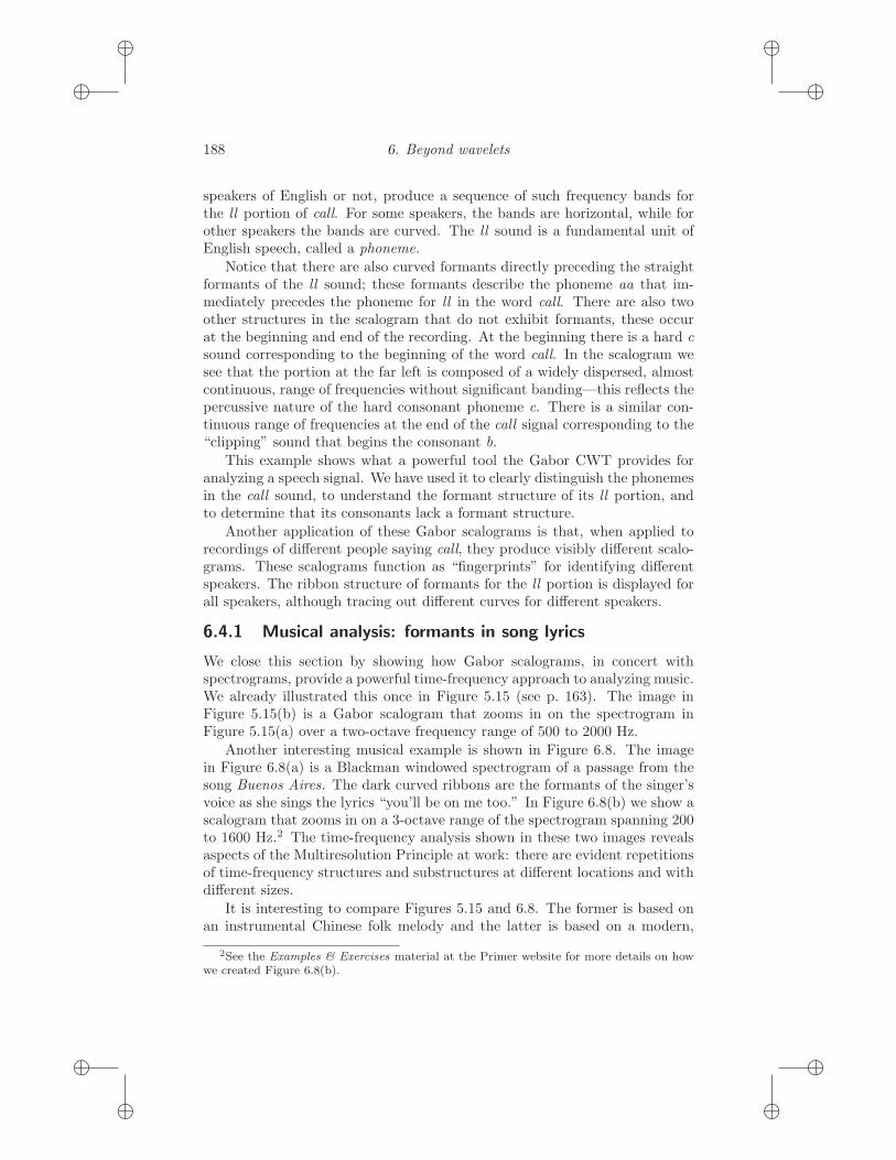
bands correspond to frequencies on a harmonic (musical) scale. In fact, inFigure 6.7(b) we show a graph of the spectrum of a sound clip of the ll

portion of the call signal. This spectrum shows that the frequencies of peakenergy in the ll portion have the following approximate values:

124, 248, 372, 496, 620, 744, 868, 992. (6.16)

Notice that these frequencies have the same ratios to the lowest frequency of124 as the ratios in (6.15) [and that 124 ≈ 80 · 20.625, . . . , 992 ≈ 80 · 23.625].

This region of the scalogram illustrates an important property of manyportions of speech signals, the property of frequency banding. These frequencybands are called formants in linguistics. All speakers, whether they are native

0 0.046 0.093 0.139 0.186−180

−90

0

90

180

(a)

0 248 496 744 992−1

0

1

2

3

(b)

FIGURE 6.7(a) A portion of the ll sound in the call signal; the horizontal axis is the timeaxis. (b) Spectrum of signal in (a); the horizontal axis is the frequency axis.

i

i

i

i

i

i

i

i


speakers of English or not, produce a sequence of such frequency bands forthe ll portion of call. For some speakers, the bands are horizontal, while forother speakers the bands are curved. The ll sound is a fundamental unit ofEnglish speech, called a phoneme.

Notice that there are also curved formants directly preceding the straightformants of the ll sound; these formants describe the phoneme aa that im-mediately precedes the phoneme for ll in the word call. There are also twoother structures in the scalogram that do not exhibit formants, these occurat the beginning and end of the recording. At the beginning there is a hard c

sound corresponding to the beginning of the word call. In the scalogram wesee that the portion at the far left is composed of a widely dispersed, almostcontinuous, range of frequencies without significant banding—this reflects thepercussive nature of the hard consonant phoneme c. There is a similar con-tinuous range of frequencies at the end of the call signal corresponding to the“clipping” sound that begins the consonant b.

This example shows what a powerful tool the Gabor CWT provides foranalyzing a speech signal. We have used it to clearly distinguish the phonemesin the call sound, to understand the formant structure of its ll portion, andto determine that its consonants lack a formant structure.

Another application of these Gabor scalograms is that, when applied torecordings of different people saying call, they produce visibly different scalo-grams. These scalograms function as “fingerprints” for identifying differentspeakers. The ribbon structure of formants for the ll portion is displayed forall speakers, although tracing out different curves for different speakers.

6.4.1 Musical analysis: formants in song lyrics

We close this section by showing how Gabor scalograms, in concert withspectrograms, provide a powerful time-frequency approach to analyzing music.We already illustrated this once in Figure 5.15 (see p. 163). The image inFigure 5.15(b) is a Gabor scalogram that zooms in on the spectrogram inFigure 5.15(a) over a two-octave frequency range of 500 to 2000 Hz.

Another interesting musical example is shown in Figure 6.8. The imagein Figure 6.8(a) is a Blackman windowed spectrogram of a passage from thesong Buenos Aires. The dark curved ribbons are the formants of the singer’svoice as she sings the lyrics “you’ll be on me too.” In Figure 6.8(b) we show ascalogram that zooms in on a 3-octave range of the spectrogram spanning 200to 1600 Hz.2 The time-frequency analysis shown in these two images revealsaspects of the Multiresolution Principle at work: there are evident repetitionsof time-frequency structures and substructures at different locations and withdifferent sizes.

It is interesting to compare Figures 5.15 and 6.8. The former is based onan instrumental Chinese folk melody and the latter is based on a modern,

2See the Examples & Exercises material at the Primer website for more details on howwe created Figure 6.8(b).

i

i

i

i

i

i

i

i

6.5 Percussion scalograms & musical rhythm 189

(a)200

566

1600

(b)

FIGURE 6.8Time-frequency analysis of a passage from the song Buenos Aires. (a) Spectro-gram. (b) Zooming in on three octaves of the frequency range of (a).

popular English song lyric. Notice that there is some similarity between thesmall angular structures: in the latter case, they are formants of the singer’svoice; in the former case, they are “pitch excursions” of a Chinese stringedinstrument that extends the power and range of human voice.

6.5 Percussion scalograms & musical rhythm

For our final discussion of the Primer, we describe how time-frequency meth-ods can be used to analyze musical rhythm. In particular, we show how anew technique known as percussion scalograms makes use of both spectro-grams and scalograms to analyze the multiple time-scales occurring withinthe rhythms of a percussion performance.

Our discussion will focus on two percussion sequences. The first sequenceis an introductory passage from the song, El Matador, which is saved as the fileel_matador_percussion_clip.wav at the Primer website. Listening to thisfile you will hear a relatively simple rhythm of drum beats, with one short shiftin tempo, and with several whistle blowings as accompaniment. We shall usethis passage to illustrate the basic principles underlying our approach. Thesecond sequence, which will show the power of our method, is a complex Latinpercussion passage that introduces the song Buenos Aires. This passage issaved in the file Buenos Aires percussion clip.wav at the Primer website.Listening to this file you will hear a richly structured percussion performancewith several tempo shifts (as well as some high pitch background sound). Ourpercussion scalogram method will produce an objective description of thesetempo shifts that accords well with our aural perception.

To derive our percussion scalogram method for analyzing drum rhythms,we consider the percussion sequence from the beginning of El Matador. InFigure 6.9(a) we show its spectrogram. This spectrogram is mostly composed

i

i

i

i

i

i

i

i


(a) Passage from El Matador (b) Passage from Buenos Aires

FIGURE 6.9Spectrograms from two percussion sequences.

of a sequence of thick vertical segments, which we will call vertical swatches.3

Each vertical swatch corresponds to a percussive strike on a drum. Thesesharp strikes on drum heads excite a continuum of frequencies rather than adiscrete tonal sequence of fundamentals and overtones. The rapid onset anddecay of these strike sounds produces vertical swatches in the time-frequencyplane. A more complex pattern of thinner vertical swatches can be seen inthe spectrogram of the Buenos Aires percussion passage in Figure 6.9(b).

Our percussion scalogram method has the following two parts:

I. Pulse train generation. We generate a “pulse train,” a sequence of al-ternating intervals of 1-values and 0-values (see the bottom graph inFigure 6.10). The location and duration of the intervals of 1-values cor-responds to our hearing of the drum strikes, and the location and durationof the intervals of 0-values corresponds to the silences between the strikes.In Figure 6.10, the rectangular-shaped pulses correspond to sharp onsetand decay of transient bursts in the percussion signal graphed just abovethe pulse train. The widths of these pulses are approximately equal tothe widths of the vertical swatches shown in the spectrogram (we graphedonly a portion of the spectrogram that omits the blotches from the whis-tle blowings, so as to isolate just the drum strikings). In Steps 1 and 2of the method below we describe how this pulse train is generated.

II. Gabor CWT. We use a Gabor CWT to analyze the pulse train. Therationale for doing this is that the pulse train is a step function analog of asinusoidal of varying frequency. Because of this rough correlation betweentempo of pulses in a pulse train and frequency in sinusoidal curves, we

3The whistle blowings correspond to three rectangular blotches at the left center of thespectrogram.

i

i

i

i

i

i

i

i


1

0

FIGURE 6.10Pulse Train for the El Matador percussion sequence.

employ a Gabor CWT for analysis.4 For example, see Figure 6.11. Thethick vertical line segments in the top half of the scalogram correspondto the drum strikes, and there is a connecting region at the bottom ofthree of the segments (the 6th, 7th, and 8th segments counting from theleft). When listening to the passage we hear those three strikes as a groupwith a clearly defined tempo shift.5 This CWT calculation is performedin Step 3 of the method.

Now that we have outlined the basis for the percussion scalogram method, wecan list it in detail. The percussion scalogram method for analyzing percussiverhythm consists of the following three steps.

Percussion Scalogram Method

Step 1. Compute a signal consisting of averages of the Gabor transform

square-magnitudes for horizontal slices lying within a frequency range

that consists mostly of vertical swatches. For the time intervals corre-sponding to vertical swatches in the spectrogram (for example, as shownin Figure 6.10) this step will produce higher square-magnitude valuesthat lie above the mean of all square-magnitudes (because the mean ispulled down by the intervals of silence). For the El Matador sequence,the frequency range of 2500 to 4500 Hz was used, as it consists mostly

4In his thesis [18], Leigh M. Smith provides a thorough empirical study of the efficacyof using Gabor CWTs to analyze percussive pulse trains.

5An important feature of the FAWAV program used to generate this percussion scalogramis that the sound file can be played and a cursor will travel across the percussion scalogram,confirming our statements about the meaning of its features. More details on how to dothis are given in the Examples & Exercises material at the Primer website.

i

i

i

i

i

i

i

i


0 1.486 2.972 sec

1

4 strikes

sec

16

FIGURE 6.11Rhythmic analysis of El Matador percussion sequence. The percussion sequenceis graphed on top, and below it is its percussion scalogram using 4 octaves, 64voices, width 0.5, freq. 0.5 (obtained from the frequency range 2500 to 4500 Hzof its spectrogram).

of the vertical swatches corresponding to the percussive strikes. (Note:In a purely percussive passage, containing only drum strikes without anybackground sounds, the complete frequency range can be used.)

Step 2. Compute a signal that is 1 whenever the signal from Step 1 is

larger than its mean and 0 otherwise. As the discussion in Step 1 shows,this will produce a pulse train whose intervals of 1-values mark off theposition and duration of the vertical swatches (hence of the drum strikes).Figure 6.10 illustrates this clearly.

Step 3. Compute a Gabor CWT of the pulse train signal from Step 2.

As we shall now discuss, this Gabor CWT provides an objective pictureof the varying rhythms within a percussion performance.

We have already discussed the Gabor CWT shown in Figure 6.11 for theEl Matador percussion sequence. The only points we want to add to thatdiscussion are some details on the meanings of the parameters used for theGabor CWT. To create the Gabor CWT in Figure 6.11, we used a widthparameter of 0.5 and a frequency parameter of 0.5. That yields a base fre-quency of 1.0 strikes/sec. The range of 4 octaves that we used then givesan upper frequency value of 16 strikes/sec.6 Notice that the vertical bars inthe scalogram in Figure 6.11 are centered on a frequency value of about 6 or7 strikes/sec and that corresponds to the number of strikes that one detects

6These CWT parameter values were obtained empirically. An apriori (automatic) selec-tion method is the subject of current research. See the preprint [22].

i

i

i

i

i

i

i

i


within any given 1 second interval; this illustrates that it is correct to inter-pret the vertical axis for the scalogram as an (octave-scaled) frequency axisof strikes/sec.

6.5.1 Analysis of a complex percussive rhythm

As an illustration of the power of our method, we use a percussion scalogramto analyze the complex rhythms of the opening percussion passage from theBuenos Aires song. See Figure 6.12. To isolate the percussive sounds, thedrum strikes, from the rest of the sounds in the passage, we used a frequencyrange of 2000 to 3000 Hz in Step 1 of the percussion scalogram method. Theparameters of the Gabor CWT are specified in the caption of Figure 6.12.

As with the El Matador sequence, it helps to play the recording of thepercussion passage and watch the cursor trace over the percussion scalogram.After listening a couple of times, and watching the cursor run along the topof the scalogram, you should find that the thin vertical strips at the top ofthe scalogram correspond to the individual drum strikes. What is even moreinteresting, however, is that several of these vertical strips bind together intolarger blobs lower down on the frequency scale (for instance, the blobs abovethe labels γ1 to γ5 in the figure). If you listen again to the recording andwatch the cursor as it passes these blobs γ1 to γ5, you will notice that thestrikes occur in groups that correspond precisely to these blobs. Furthermore,the blobs γ3 to γ5 are connected together, and one does perceive a largertime-scale grouping of percussion strikes over the time-interval covered bythese three blobs. Finally, we note that there is another collection of blobs tothe right of γ5. We have not labeled them, but we leave it to the reader toinfer the connection between them and the shifting pattern of drum strikesin the recording. Notice, however, that these blobs appear to be linked to alarger region, labeled Γ, which provides an objective description of our auralperception of the further grouping of these collections of drum strikes.

6.5.2 Multiresolution Principle for rhythm

Our discussion of these two percussion sequences illustrates the fact that theMultiresolution Principle for tonal music that we introduced on p. 160—thepatterning of time-frequency structures over multiple time-scales—also appliesto rhythmic percussion. We can even see the three representations describedby Pinker (p. 164) applying as well, if we substitute “strikes” for “notes.” Forexample, the single strikes are grouped into blobs, and some of these blobsare joined together into longer groups. This multiresolution time-frequencypatterning, captured by our percussion scalograms, may be useful in charac-terizing different styles of percussion. But that is a subject for future research.

i

i

i

i

i

i

i

i


0 4.096 8.192 sec

γ1

γ2

γ3 γ4 γ5

Γ

0.5

2.38 strikes

sec

16

FIGURE 6.12Rhythmic analysis of Buenos Aires percussion sequence. The percussion se-quence is graphed on top, and below it is its percussion scalogram using 5octaves, 51 voices, width 2, freq. 1 (obtained from the frequency range 2000 to3000 Hz of its spectrogram). The labels are explained in the text.

6.6 Notes and References

The best introductory material on wavelet packet transforms can be found in[2] and [3]. There is also a good discussion in [4]. A very thorough treatmentof the subject is given in [5]. The relation between wavelet packet transformsand the WSQ method is described in [6], and the wavelet packet transformoption allowed by JPEG 2000 Part 2 is described in [7].

Rigorous expositions of the complete theory of CWTs can be found in [8]and [9]. A more complete treatment of the discrete version described in thisprimer is given in [10].

For a discussion of the uses of the CWT for analysis of ECGs, see [11] and[12]. In addition to an excellent discussion of the topic, [12] also contains anextensive bibliography.

Applying Gabor CWTs to the detection of engine malfunctions in Japaneseautomobiles is described in [13]. An interesting relationship between CWTsand human hearing, with applications to speech analysis, is described in [14].Background on formants and phonemes in linguistics can be found in [15].

Scalograms are used, in conjunction with spectrograms, to provide analysisof music and musical instruments in [16] and [17]. An empirical discussionof percussive rhythm and applications is given by Leigh Smith in [18]. Someother papers on related topics can be found on his webpage [19]. WilliamSethares has done profound work on computerized rhythm analysis [20], [21].

i

i

i

i

i

i

i

i

6.6 Notes and References 195

The preprint [22] describes an alternative approach to this same topic.

6.6.1 Additional References

We now provide references for some additional topics that extend the discus-sion in the text. These topics are (1) best basis algorithms, (2) local cosineseries, (3) frames, (4) curvelets, (5) 3D wavelets, and (6) video compression.

Best basis algorithms. There are algorithms that choose which fluctuationsubsignals to decompose further (by wavelet transform) according to someminimization of a cost function. An excellent introduction to such a bestbasis algorithm, and its application to the WSQ algorithm, can be found inDavid Walnut’s book [23]. A complete discussion, by the discoverer of thetechnique, is in [5].

Local cosine series. The Gabor transform discussed in Chapter 5 has beencriticized for its reliance on windows of constant size. A method which allowsfor windows of varying size, as well as using real-valued cosine functions, isthe method of local cosine series. Local cosine series have proven to be quiteuseful in compression of signals. An elementary discussion can be found inChapter 2 of [24]. See also the paper by Auscher et al in [25], and the treatmentin [5]. A related area to local cosine series are the fields of lapped orthogonal

transforms and generalized lapped orthogonal transforms (GenLOT). Thesefields are described in [26] to [30].

Frames. The inversion of Gabor transforms discussed in Chapter 5 providesone class of expansions of signals using frames. Frames have proven to beespecially useful in denoising applications. See [31] to [35]. References [36]and [37] provide fundamental mathematical background.

Curvelets. David Donoho and his collaborators have done extensive work ona generalization of wavelets for image processing known as curvelets. Curveletsprovide for efficient modelling of edges in images. See the papers [38] to [40],and also the website [41].

3D wavelets. Wim Sweldens and his collaborators have done a lot of workon wavelets and their generalizations in 3D. See [42] and [43], and the website[44]. Curvelets have also been adapted for 3D processing [45].

Video compression. A good synopsis of the basics of wavelet-based videocompression can be found in [10]. Important work in the field is being doneby Truong Nguyen’s group, see [46] for many downloadable publications.

1. B. Burke. (1994). The Mathematical Microscope: waves, wavelets, and beyond.In A Positron Named Priscilla, Scientific Discovery at the Frontier, M. Bartu-siak (Ed.), 196–235, National Academy Press.

2. M.V. Wickerhauser. (1993). Best-adapted Wavelet Packet Bases. In DifferentPerspectives on Wavelets, I. Daubechies (Ed.), AMS, Providence, RI, 155–172.

i

i

i

i

i

i

i

i


3. R.R. Coifman, M.V. Wickerhauser. (1993). Wavelets and Adapted WaveformAnalysis. A Toolkit for Signal Processing and Numerical Analysis. In DifferentPerspectives on Wavelets, I. Daubechies (Ed.), AMS, Providence, RI, 119–154.

4. R.R. Coifman and M.V. Wickerhauser. (1994). Wavelets and Adapted WaveformAnalysis. In Wavelets. Mathematics and Applications, J. Benedetto, M. Fra-zier (Eds.), CRC Press, Boca Raton, FL, 399–424.

5. M.V. Wickerhauser. (1994). Adapted Wavelet Analysis from Theory to Software.A.K. Peters, Wellesley, MA, 1994.

6. J.N. Bradley, C.M. Brislawn, T. Hopper. (1993). The FBI Wavelet/Scalar Quan-tization Standard for gray-scale fingerprint image compression. SPIE, Vol. 1961,Visual Information Processing II (1993), 293–304.

7. D.S. Taubman and M.W. Marcellin. (2002). JPEG2000: Image compressionfundamentals, standards and practice. Kluwer, Boston, MA.

8. I. Daubechies. (1992). Ten Lectures on Wavelets. SIAM, Philadelphia, PA.

9. A.K. Louis, P. Maaß, A. Rieder. (1997). Wavelets, Theory and Applications.Wiley, New York, NY.

10. S. Mallat. (1999). A Wavelet Tour of Signal Processing. Second Edition. Aca-demic Press, New York, NY.

11. L. Senhadji, L. Thoraval, G. Carrault. (1996). Continuous Wavelet Transform:ECG Recognition Based on Phase and Modulus Representations and HiddenMarkov Models. In Wavelets in Medicine and Biology, A. Aldroubi, M. Unser(Eds.), CRC Press, Boca Raton, FL, 439–464.

12. P.S. Addison. (2005). Wavelet transforms and the ECG: a review. Phys-iol. Meas., Vol. 26, R155–R199.

13. M. Kobayashi. (1996). Listening for Defects: Wavelet-Based Acoustical SignalProcessing in Japan. SIAM News, Vol. 29, No. 2.

14. I. Daubechies and S. Maes. (1996). A Nonlinear Squeezing of the ContinuousWavelet Transform Based on Auditory Nerve Models. In Wavelets in Medicineand Biology, A. Aldroubi, M. Unser (Eds.), CRC Press, Boca Raton, FL, 527–546.

15. W. O’Grady, M. Dobrovolsky, M. Arnoff. (1993). Contemporary Linguistics, AnIntroduction. St. Martins Press, New York.

16. J.S. Walker and G.W. Don. (2006). Music: a time-frequency approach. Sub-mitted. Available at http://www.uwec.edu/walkerjs/media/TFAM.pdf

17. J.F. Alm and J.S. Walker. (2002). Time-frequency analysis of musical instru-ments. SIAM Review, Vol. 44, 457–476.

18. L.M. Smith (2000). A multiresolution time-frequency analysis and interpretationof musical rhythm. Thesis, University of Western Australia.

19. L.M. Smith’s webpage: http://staff.science.uva.nl/~lsmith/

20. W. Sethares. (2007). Rhythm and Transforms. Springer, New York, NY.

21. W. Sethares. (2007). Rhythm and Transforms. An extended abstract of hisplenary address to the Mathematics and Computation in Music conference inBerlin, May 18, 2007. Available at

http://www.mcm2007.info/pdf/fri1-sethares.pdf

i

i

i

i

i

i

i

i

6.6 Notes and References 197

22. X. Cheng, J.V. Hart, J.S. Walker. (2007). Time-frequency analysis of musicalrhythm. Preprint. Available at

http://www.uwec.edu/walkerjs/media/TFAMR.pdf

23. D.F. Walnut. (2002). An Introduction to Wavelet Analysis. Birkhauser, Boston,MA.

24. E. Hernandez, G. Weiss. (1996). A First Course on Wavelets. CRC Press, BocaRaton, FL.

25. C.K. Chui (Ed.) (1992). Wavelets: a tutorial in theory and applications. Aca-demic Press, Boston, MA.

26. H.S. Malvar, D.H. Staelin. (1989). The LOT: transform coding without blockingeffects. IEEE Transactions on Acoustics, Speech, and Signal Processing, Vol. 37,553-559.

27. T.Q. Nguyen. (1992). A class of generalized cosine-modulated filter bank. Pro-ceedings 1992 IEEE International Symposium on Circuits and Systems, Vol. 2,943–946.

28. R.L. de Queiroz, T.Q. Nguyen, K.R. Rao. (1996). The GenLOT: generalizedlinear-phase lapped orthogonal transform. IEEE Transactions on Signal Pro-cessing, Vol. 44, 497–507.

29. S. Oraintara, P. Heller, T. Tran, and T. Nguyen. (2001). Lattice structure forregular paraunitary linear-phase filterbanks and M-band orthogonal symmetricwavelets. IEEE Transactions on Signal Processing, Vol. 49, 2659-2672.

30. Y.-J. Chen, S. Oraintara, K. Amaratunga. (2005). Dyadic-based factorizationfor regular paraunitary filter banks and M-band orthogonal wavelets with struc-tural vanishing moments. IEEE Transactions on Signal Processing, Vol. 53,193–207.

31. R. Coifman and Y. Zeevi, Eds. (1988). Signal and Image Representation inCombined Spaces. Wavelet Analysis and Applications, Vol. 7, Academic Press,Boston, MA.

32. I. Daubechies. (1992). Ten Lectures on Wavelets. SIAM, Philadelphia, PA.

33. H. Feichtinger and T. Strohmer, Eds. (1998). Gabor Analysis and Algorithms.Birkhauser, Boston, MA.

34. H. Feichtinger and T. Strohmer, Eds. (2002). Advances in Gabor Analysis.Birkhauser, Boston, MA.

35. R. Young. (1980). An Introduction to Nonharmonic Fourier Series. AcademicPress, New York, NY.

36. P.G. Casazza. (2000). The Art of Frame Theory. Taiwanese J. of Mathematics,Vol. 4, 129–201.

37. B.D. Johnson. (2002). Wavelets: generalized quasi-affine and oversampled-affineframes. Thesis, Washington University in St. Louis.

38. D. Donoho and A.G. Flesia. (2001). Can recent innovations in harmonic analysis‘explain’ key findings in natural image statistics? Network Computations inNeural Systems, Vol. 12, 371–393.

i

i

i

i

i

i

i

i


39. D. Donoho and E. Candes. (2005). Continuous Curvelet Transform I: Resolutionof Wavefront Set. Applied and Computational Harmonic Analysis, Vol. 19, 162–197.

40. D. Donoho and E. Candes. (2005). Continuous Curvelet Transform II: Dis-cretization and Frames. Appl. Comput. Harmon. Anal. Vol. 19, 198–222.

41. Curvelet website: http://www.curvelet.org/papers.html

42. A. Khodakovsky, P. Schroder, and W. Sweldens. (2000). Progressive GeometryCompression. SIGGRAPH 2000, 271–278.

43. I. Guskov, W. Sweldens, and P. Schroder. (1999). Multiresolution Signal Pro-cessing for Meshes. SIGGRAPH 1999, 325-334.

44. W. Swelden’s papers: netlib.bell-labs.com/cm/ms/who/wim/papers/

45. L. Ying, L. Demanet, E. J. Candes. (2005). 3D Discrete Curvelet Transform.Proceedings of SPIE—Volume 5914, Wavelets XI, M. Papadakis, A.F. Laine,M.A. Unser (Eds.).

46. UCSD Video Processing page: http://videoprocessing.ucsd.edu/

6.3 continuous wavelet transforms · scalogram of this signal using a mexican hat wavelet of width...

Documents