6 applying logistic regression models - nc state universitydzhang2/st744/chap6.pdf · 6 applying...
TRANSCRIPT

CHAPTER 6 ST744, D. Zhang
6 Applying Logistic Regression Models
I Model Selection and Diagnostics
I.1 Model Selection
• # of x’s can be entered in the model:
Rule of thumb: # of events (both [Y = 1] and [Y = 0]) per x ≥ 10.
• Need to be aware of collinearity in x’s.
• Use traditional model selection procedures (used when p << n)
1. Forward selection (simple one + variant)
2. Backward elimination
• Use modern model selection procedures, usually in the form of
penalized likelihood (can handle p > n); New research area.
Slide 344
CHAPTER 6 ST744, D. Zhang
• Use LRT for nested models (e.g., Table 6.2)
• Use AIC (Akaike information criterion) or BIC (Bayesian information
criterion) for model selection (not necessarily nested models)
AIC = −2{ℓmax − p}BIC = −2{ℓmax − 0.5 log(n)p}
Smaller AIC/BIC, the better.
Note: BIC tends to yield a simpler model than AIC.
• Use common sense in model building (e.g. time ordering, etc. Table
6.3).
Slide 345
CHAPTER 6 ST744, D. Zhang
I.2 Model Diagnostics
• Use standardized residuals to check model fit and identify outliers:
yi|xiind∼ Bin(ni, πi)
logit(πi) = xTi β
πi =exT
ibβ
1 + exTi
bβ
1. Standardized Pearson residual:
ei =yi − πi√niπi(1− πi)
esti =
ei√1− hi
Slide 346
CHAPTER 6 ST744, D. Zhang
2. Standardized deviance residual:
di = 2
(yi log
yi
niπi+ (ni − yi) log
ni − yi
ni − niπi
)
di =√disign(yi − πi)
dsti =
di√1− hi
• If |esti | (or |dst
i |) > 2, 3 ⇒ outliers.
• Plots of esti (or dst
i ) v.s. xi or xTi β may detect lack of fit.
• When ni = 1, esti (or dst
i ) not very informative.
• Note: Proc Logistic does not report esti and dst
i . Need to use
Proc GenMod to get esti and dst
i .
Slide 347

CHAPTER 6 ST744, D. Zhang
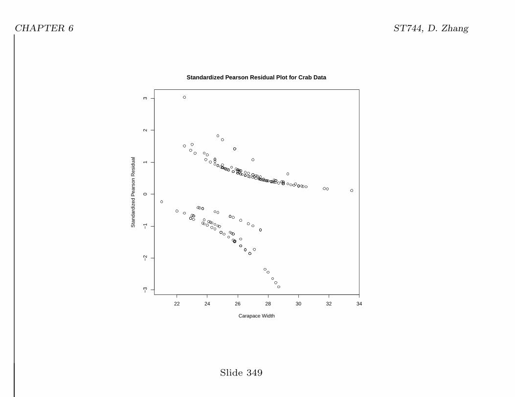
• Example 1: Residual plot for the crab data:
Model: logit(P [Y = 1|x, c]) = β0 + β1c1 + β2c2 + β3c3 + β4xdata crab;
input color spine width satell weight;weight=weight/1000;color=color-1;satbin=(satell>0);c1 = (color=1);c2 = (color=2);c3 = (color=3);c4 = (color=4);s1 = (spine=1);s2 = (spine=2);datalines;
3 3 28.3 8 30504 3 22.5 0 15502 1 26.0 9 23004 3 24.8 0 21004 3 ...
proc genmod data=crab descending;model satbin = width c1 c2 c3 / dist=bin link=logit;output out=resid ResRaw=ResRaw ResChi=ResChi StdReschi=StdReschi;
run;
data _null_; set resid;file "crab_res";put stdreschi width;
run;
Slide 348
CHAPTER 6 ST744, D. Zhang
22 24 26 28 30 32 34
−3
−2
−1
01
23
Carapace Width
Sta
ndar
dize
d P
ears
on R
esid
ual
Standardized Pearson Residual Plot for Crab Data
Slide 349
CHAPTER 6 ST744, D. Zhang
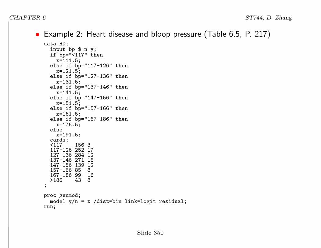
• Example 2: Heart disease and bloop pressure (Table 6.5, P. 217)data HD;
input bp $ n y;if bp="<117" thenx=111.5;
else if bp="117-126" thenx=121.5;
else if bp="127-136" thenx=131.5;
else if bp="137-146" thenx=141.5;
else if bp="147-156" thenx=151.5;
else if bp="157-166" thenx=161.5;
else if bp="167-186" thenx=176.5;
elsex=191.5;
cards;<117 156 3117-126 252 17127-136 284 12137-146 271 16147-156 139 12157-166 85 8167-186 99 16>186 43 8
;
proc genmod;model y/n = x /dist=bin link=logit residual;
run;
Slide 350
CHAPTER 6 ST744, D. Zhang
Criteria For Assessing Goodness Of Fit
Criterion DF Value Value/DF
Deviance 6 5.9092 0.9849Scaled Deviance 6 5.9092 0.9849Pearson Chi-Square 6 6.2899 1.0483Scaled Pearson X2 6 6.2899 1.0483
Analysis Of Maximum Likelihood Parameter Estimates
Standard Wald 95% Confidence WaldParameter DF Estimate Error Limits Chi-Square
Intercept 1 -6.0820 0.7243 -7.5017 -4.6624 70.51x 1 0.0243 0.0048 0.0148 0.0338 25.25
Raw Pearson DevianceObservation Residual Residual Residual
Std Deviance Std Pearson LikelihoodResidual Residual Residual
1 -2.194866 -0.979434 -1.061683-1.198648 -1.105788 -1.179257
2 6.3932374 2.0057053 1.85010722.1903838 2.3745999 2.2447199
3 -3.072737 -0.813338 -0.841966-0.978546 -0.945274 -0.970016
4 -2.081617 -0.50673 -0.51623-0.583485 -0.572747 -0.581169
5 0.3836399 0.1175816 0.11700160.1254648 0.1260868 0.1255461
6 -0.856987 -0.304247 -0.308775-0.330927 -0.326074 -0.330303
7 1.791237 0.5134723 0.50496570.6411542 0.651955 0.6452766
8 -0.361958 -0.139464 -0.140243-0.178337 -0.177346 -0.177959
Slide 351
CHAPTER 6 ST744, D. Zhang
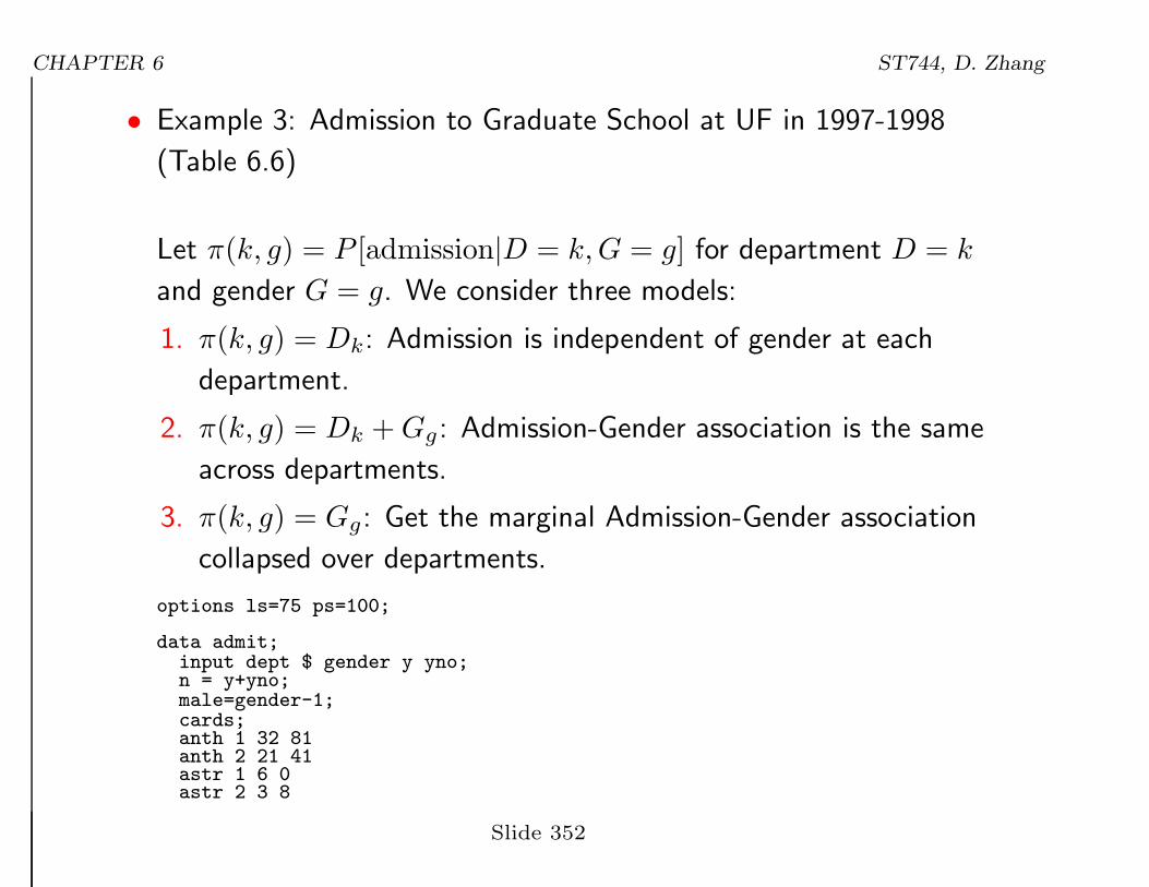
• Example 3: Admission to Graduate School at UF in 1997-1998
(Table 6.6)
Let π(k, g) = P [admission|D = k,G = g] for department D = k
and gender G = g. We consider three models:
1. π(k, g) = Dk: Admission is independent of gender at each
department.
2. π(k, g) = Dk +Gg: Admission-Gender association is the same
across departments.
3. π(k, g) = Gg: Get the marginal Admission-Gender association
collapsed over departments.
options ls=75 ps=100;
data admit;input dept $ gender y yno;n = y+yno;male=gender-1;cards;anth 1 32 81anth 2 21 41astr 1 6 0astr 2 3 8
Slide 352

CHAPTER 6 ST744, D. Zhang
chem 1 12 43chem 2 34 110...
title "Model 1: Logistic model assuming gender and admission are";title2 "conditional independent given department";proc genmod;
class dept;model y/n = dept /dist=bin link=logit;output out=resid Resraw=Resraw Reschi=Reschi StdReschi=StdReschi;
run;
data resid; set resid;keep dept male Resraw Reschi StdReschi;
run;
title "Residuals from Model 1";proc print data=resid;run;
title "Model 2: Logistic model with homogeneous GA and DA association";proc genmod data=admit;
class dept;model y/n = dept male;
run;
title "Model 3: Logistic model for marginal GA association";proc genmod data=admit;
model y/n = male;run;
Slide 353
CHAPTER 6 ST744, D. Zhang
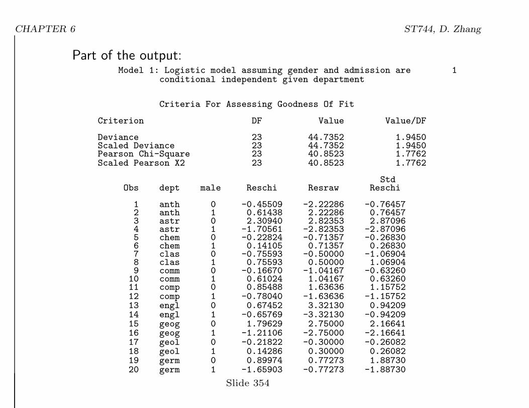
Part of the output:Model 1: Logistic model assuming gender and admission are 1
conditional independent given department
Criteria For Assessing Goodness Of Fit
Criterion DF Value Value/DF
Deviance 23 44.7352 1.9450Scaled Deviance 23 44.7352 1.9450Pearson Chi-Square 23 40.8523 1.7762Scaled Pearson X2 23 40.8523 1.7762
StdObs dept male Reschi Resraw Reschi
1 anth 0 -0.45509 -2.22286 -0.764572 anth 1 0.61438 2.22286 0.764573 astr 0 2.30940 2.82353 2.870964 astr 1 -1.70561 -2.82353 -2.870965 chem 0 -0.22824 -0.71357 -0.268306 chem 1 0.14105 0.71357 0.268307 clas 0 -0.75593 -0.50000 -1.069048 clas 1 0.75593 0.50000 1.069049 comm 0 -0.16670 -1.04167 -0.6326010 comm 1 0.61024 1.04167 0.6326011 comp 0 0.85488 1.63636 1.1575212 comp 1 -0.78040 -1.63636 -1.1575213 engl 0 0.67452 3.32130 0.9420914 engl 1 -0.65769 -3.32130 -0.9420915 geog 0 1.79629 2.75000 2.1664116 geog 1 -1.21106 -2.75000 -2.1664117 geol 0 -0.21822 -0.30000 -0.2608218 geol 1 0.14286 0.30000 0.2608219 germ 0 0.89974 0.77273 1.8873020 germ 1 -1.65903 -0.77273 -1.88730
Slide 354
CHAPTER 6 ST744, D. Zhang
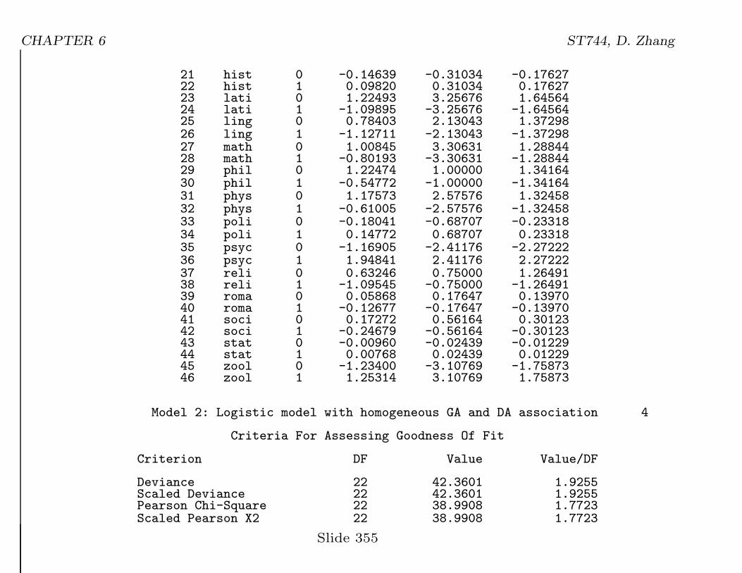
21 hist 0 -0.14639 -0.31034 -0.1762722 hist 1 0.09820 0.31034 0.1762723 lati 0 1.22493 3.25676 1.6456424 lati 1 -1.09895 -3.25676 -1.6456425 ling 0 0.78403 2.13043 1.3729826 ling 1 -1.12711 -2.13043 -1.3729827 math 0 1.00845 3.30631 1.2884428 math 1 -0.80193 -3.30631 -1.2884429 phil 0 1.22474 1.00000 1.3416430 phil 1 -0.54772 -1.00000 -1.3416431 phys 0 1.17573 2.57576 1.3245832 phys 1 -0.61005 -2.57576 -1.3245833 poli 0 -0.18041 -0.68707 -0.2331834 poli 1 0.14772 0.68707 0.2331835 psyc 0 -1.16905 -2.41176 -2.2722236 psyc 1 1.94841 2.41176 2.2722237 reli 0 0.63246 0.75000 1.2649138 reli 1 -1.09545 -0.75000 -1.2649139 roma 0 0.05868 0.17647 0.1397040 roma 1 -0.12677 -0.17647 -0.1397041 soci 0 0.17272 0.56164 0.3012342 soci 1 -0.24679 -0.56164 -0.3012343 stat 0 -0.00960 -0.02439 -0.0122944 stat 1 0.00768 0.02439 0.0122945 zool 0 -1.23400 -3.10769 -1.7587346 zool 1 1.25314 3.10769 1.75873
Model 2: Logistic model with homogeneous GA and DA association 4
Criteria For Assessing Goodness Of Fit
Criterion DF Value Value/DF
Deviance 22 42.3601 1.9255Scaled Deviance 22 42.3601 1.9255Pearson Chi-Square 22 38.9908 1.7723Scaled Pearson X2 22 38.9908 1.7723
Slide 355
CHAPTER 6 ST744, D. Zhang
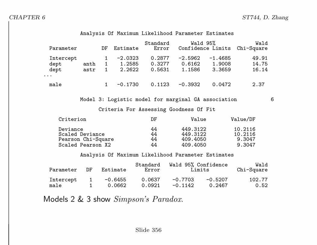
Analysis Of Maximum Likelihood Parameter Estimates
Standard Wald 95% WaldParameter DF Estimate Error Confidence Limits Chi-Square
Intercept 1 -2.0323 0.2877 -2.5962 -1.4685 49.91dept anth 1 1.2585 0.3277 0.6162 1.9008 14.75dept astr 1 2.2622 0.5631 1.1586 3.3659 16.14
...
male 1 -0.1730 0.1123 -0.3932 0.0472 2.37
Model 3: Logistic model for marginal GA association 6
Criteria For Assessing Goodness Of Fit
Criterion DF Value Value/DF
Deviance 44 449.3122 10.2116Scaled Deviance 44 449.3122 10.2116Pearson Chi-Square 44 409.4050 9.3047Scaled Pearson X2 44 409.4050 9.3047
Analysis Of Maximum Likelihood Parameter Estimates
Standard Wald 95% Confidence WaldParameter DF Estimate Error Limits Chi-Square
Intercept 1 -0.6455 0.0637 -0.7703 -0.5207 102.77male 1 0.0662 0.0921 -0.1142 0.2467 0.52
Models 2 & 3 show Simpson’s Paradox.
Slide 356
CHAPTER 6 ST744, D. Zhang
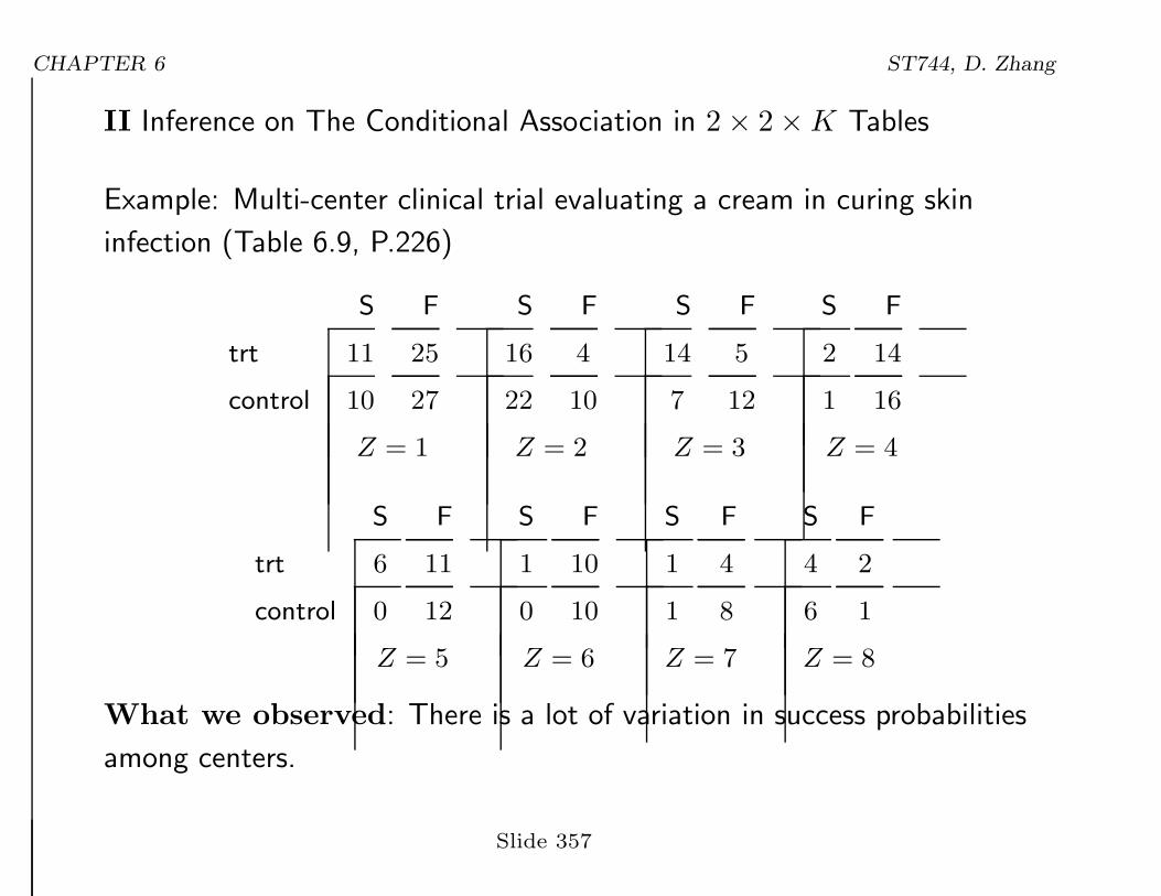
II Inference on The Conditional Association in 2× 2×K Tables
Example: Multi-center clinical trial evaluating a cream in curing skin
infection (Table 6.9, P.226)
S F
trt 11 25
control 10 27
Z = 1
S F
16 4
22 10
Z = 2
S F
14 5
7 12
Z = 3
S F
2 14
1 16
Z = 4
S F
trt 6 11
control 0 12
Z = 5
S F
1 10
0 10
Z = 6
S F
1 4
1 8
Z = 7
S F
4 2
6 1
Z = 8
What we observed: There is a lot of variation in success probabilities
among centers.
Slide 357

CHAPTER 6 ST744, D. Zhang
If we collapse the tables over centers, we got:
Y
S F
X trt 55 75
control 47 96
⇒θXY =
96× 55
47× 75≈ 1.5
The above estimate θXY may not be very useful since this is not a
random sample, so we cannot use the famous formula for calculating the
variance of log θXY :
var(log θXY ) 6= 1
55+
1
75+
1
47+
1
96.
⇒ Should focus on conditional association!
Slide 358
CHAPTER 6 ST744, D. Zhang
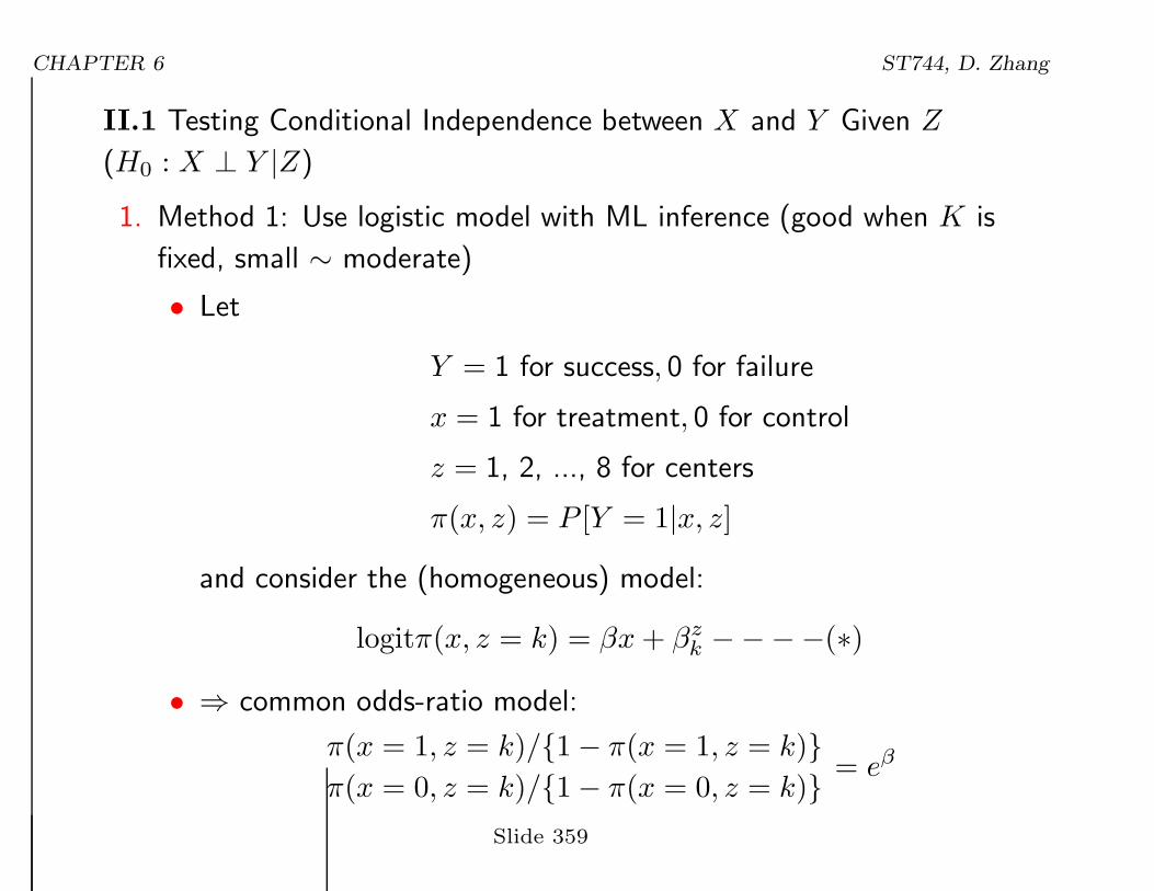
II.1 Testing Conditional Independence between X and Y Given Z
(H0 : X ⊥ Y |Z)
1. Method 1: Use logistic model with ML inference (good when K is
fixed, small ∼ moderate)
• Let
Y = 1 for success, 0 for failure
x = 1 for treatment, 0 for control
z = 1, 2, ..., 8 for centers
π(x, z) = P [Y = 1|x, z]
and consider the (homogeneous) model:
logitπ(x, z = k) = βx+ βzk −−−−(∗)
• ⇒ common odds-ratio model:
π(x = 1, z = k)/{1− π(x = 1, z = k)}π(x = 0, z = k)/{1− π(x = 0, z = k)} = eβ
Slide 359
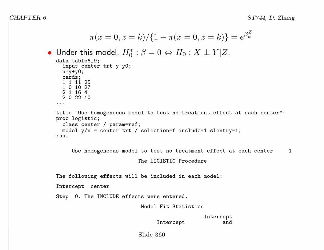
CHAPTER 6 ST744, D. Zhang
π(x = 0, z = k)/{1− π(x = 0, z = k)} = eβZk
• Under this model, H∗0 : β = 0 ⇔ H0 : X ⊥ Y |Z.
data table6_9;input center trt y y0;n=y+y0;cards;1 1 11 251 0 10 272 1 16 42 0 22 10
...
title "Use homogeneous model to test no treatment effect at each center";proc logistic;
class center / param=ref;model y/n = center trt / selection=f include=1 slentry=1;
run;
Use homogeneous model to test no treatment effect at each center 1
The LOGISTIC Procedure
The following effects will be included in each model:
Intercept center
Step 0. The INCLUDE effects were entered.
Model Fit Statistics
InterceptIntercept and
Slide 360
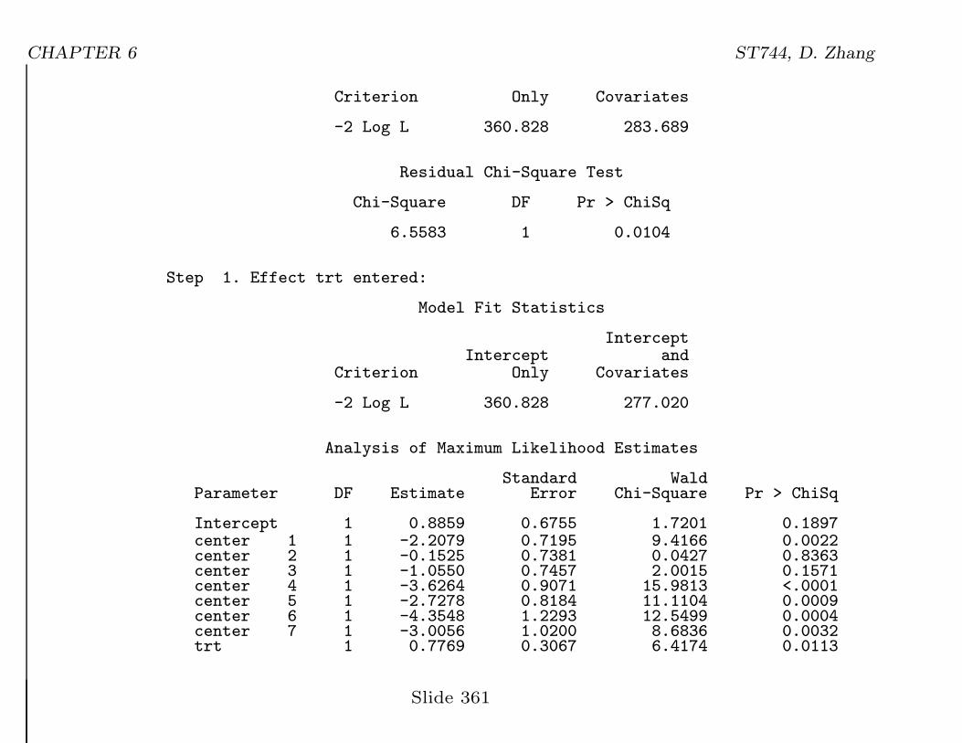
CHAPTER 6 ST744, D. Zhang
Criterion Only Covariates
-2 Log L 360.828 283.689
Residual Chi-Square Test
Chi-Square DF Pr > ChiSq
6.5583 1 0.0104
Step 1. Effect trt entered:
Model Fit Statistics
InterceptIntercept and
Criterion Only Covariates
-2 Log L 360.828 277.020
Analysis of Maximum Likelihood Estimates
Standard WaldParameter DF Estimate Error Chi-Square Pr > ChiSq
Intercept 1 0.8859 0.6755 1.7201 0.1897center 1 1 -2.2079 0.7195 9.4166 0.0022center 2 1 -0.1525 0.7381 0.0427 0.8363center 3 1 -1.0550 0.7457 2.0015 0.1571center 4 1 -3.6264 0.9071 15.9813 <.0001center 5 1 -2.7278 0.8184 11.1104 0.0009center 6 1 -4.3548 1.2293 12.5499 0.0004center 7 1 -3.0056 1.0200 8.6836 0.0032trt 1 0.7769 0.3067 6.4174 0.0113
Slide 361
CHAPTER 6 ST744, D. Zhang
• Three Tests for H0 : β = 0:
(a) Score test: χ2 = 6.5583, df = 1, P = 0.0104.
(b) LRT: G2 = 283.689− 277.020 = 6.669, df = 1, P = 0.0098.
(c) Wald test: χ2 = 6.4174, P = 0.0113.
Strong evidence to reject H0 : β = 0.
• β = 0.7769, ebβ = 2.17 ⇒ At each center, the odds of success
(infection is cured) for treated patients is 2.17 times the odds of
success for untreated patients.
• Note 1: The above test results are based on the homogeneous
model (*). When β = 0, model (*) reduces to
logitπ(x, z = k) = βzk
⇔ to H0 : X ⊥ Y |Z, can be tested by conducting the GOF test
for this model.
Slide 362
CHAPTER 6 ST744, D. Zhang
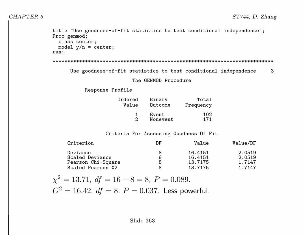
title "Use goodness-of-fit statistics to test conditional independence";Proc genmod;
class center;model y/n = center;
run;
***************************************************************************
Use goodness-of-fit statistics to test conditional independence 3
The GENMOD Procedure
Response Profile
Ordered Binary TotalValue Outcome Frequency
1 Event 1022 Nonevent 171
Criteria For Assessing Goodness Of Fit
Criterion DF Value Value/DF
Deviance 8 16.4151 2.0519Scaled Deviance 8 16.4151 2.0519Pearson Chi-Square 8 13.7175 1.7147Scaled Pearson X2 8 13.7175 1.7147
χ2 = 13.71, df = 16− 8 = 8, P = 0.089.
G2 = 16.42, df = 8, P = 0.037. Less powerful.
Slide 363
CHAPTER 6 ST744, D. Zhang
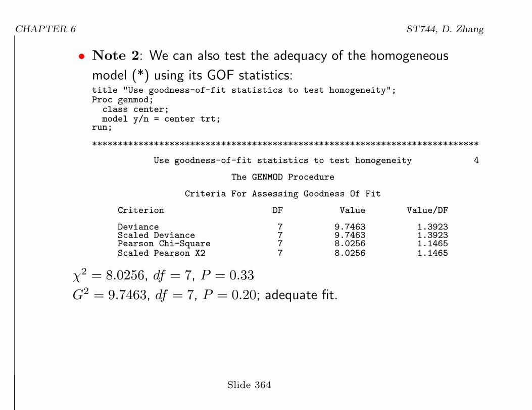
• Note 2: We can also test the adequacy of the homogeneous
model (*) using its GOF statistics:title "Use goodness-of-fit statistics to test homogeneity";Proc genmod;
class center;model y/n = center trt;
run;
***************************************************************************
Use goodness-of-fit statistics to test homogeneity 4
The GENMOD Procedure
Criteria For Assessing Goodness Of Fit
Criterion DF Value Value/DF
Deviance 7 9.7463 1.3923Scaled Deviance 7 9.7463 1.3923Pearson Chi-Square 7 8.0256 1.1465Scaled Pearson X2 7 8.0256 1.1465
χ2 = 8.0256, df = 7, P = 0.33
G2 = 9.7463, df = 7, P = 0.20; adequate fit.
Slide 364
CHAPTER 6 ST744, D. Zhang
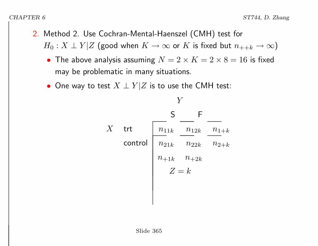
2. Method 2. Use Cochran-Mental-Haenszel (CMH) test for
H0 : X ⊥ Y |Z (good when K →∞ or K is fixed but n++k →∞)
• The above analysis assuming N = 2×K = 2× 8 = 16 is fixed
may be problematic in many situations.
• One way to test X ⊥ Y |Z is to use the CMH test:
Y
S F
X trt n11k n12k n1+k
control n21k n22k n2+k
n+1k n+2k
Z = k
Slide 365
CHAPTER 6 ST744, D. Zhang
• Under H0 : X ⊥ Y |Z, n11k|n1+k, n+1k ∼ hypergeometric
distribution:
E(n11k|H0, n1+k, n+1k) =n1+kn+1k
n++k= µ11k,
var(n11k|H0, n1+k, n+1k) =n1+kn2+kn+1kn+2k
n2++k(n++k − 1)
.
⇒χ2 =
[∑K
k=1(n11k − µ11k)]2∑K
k=1 var(n11k|H0, n1+k, n+1k)
H0∼ χ21.
• CMH with correction:
χ2c =
{|∑Kk=1(n11k − µ11k)| − 0.5}2
∑Kk=1 var(n11k|H0, n1+k, n+1k)
H0∼ χ21.
• The CMH does not require the homogeneous model.
Slide 366
CHAPTER 6 ST744, D. Zhang
data y1; set table6_9;count=y;drop y0;y=1;
run;
data y0; set table6_9;count=y0;drop y0;y=0;
run;
data new; set y1 y0;run;
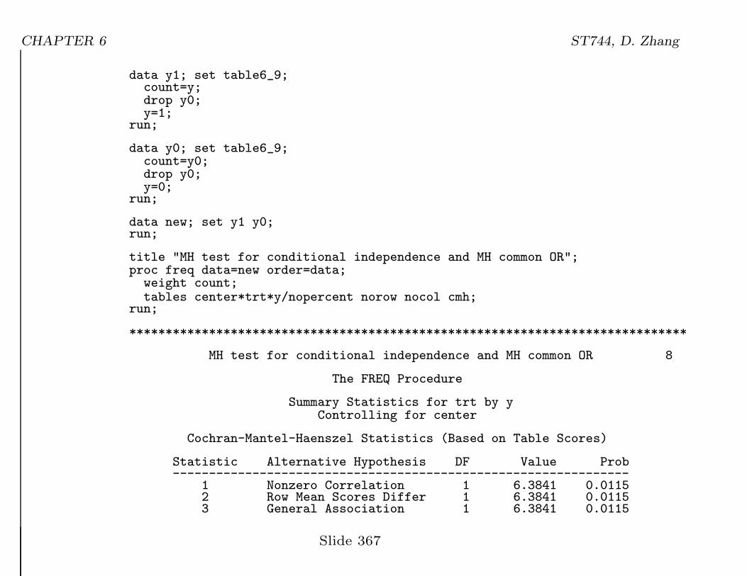
title "MH test for conditional independence and MH common OR";proc freq data=new order=data;
weight count;tables center*trt*y/nopercent norow nocol cmh;
run;
*****************************************************************************
MH test for conditional independence and MH common OR 8
The FREQ Procedure
Summary Statistics for trt by yControlling for center
Cochran-Mantel-Haenszel Statistics (Based on Table Scores)
Statistic Alternative Hypothesis DF Value Prob---------------------------------------------------------------
1 Nonzero Correlation 1 6.3841 0.01152 Row Mean Scores Differ 1 6.3841 0.01153 General Association 1 6.3841 0.0115
Slide 367
CHAPTER 6 ST744, D. Zhang
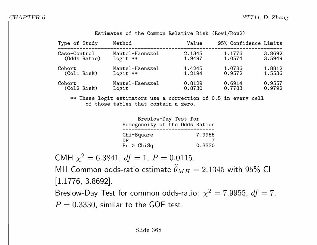
Estimates of the Common Relative Risk (Row1/Row2)
Type of Study Method Value 95% Confidence Limits-------------------------------------------------------------------------Case-Control Mantel-Haenszel 2.1345 1.1776 3.8692
(Odds Ratio) Logit ** 1.9497 1.0574 3.5949
Cohort Mantel-Haenszel 1.4245 1.0786 1.8812(Col1 Risk) Logit ** 1.2194 0.9572 1.5536
Cohort Mantel-Haenszel 0.8129 0.6914 0.9557(Col2 Risk) Logit 0.8730 0.7783 0.9792
** These logit estimators use a correction of 0.5 in every cellof those tables that contain a zero.
Breslow-Day Test forHomogeneity of the Odds Ratios------------------------------Chi-Square 7.9955DF 7Pr > ChiSq 0.3330
CMH χ2 = 6.3841, df = 1, P = 0.0115.
MH Common odds-ratio estimate θMH = 2.1345 with 95% CI
[1.1776, 3.8692].
Breslow-Day Test for common odds-ratio: χ2 = 7.9955, df = 7,
P = 0.3330, similar to the GOF test.
Slide 368
CHAPTER 6 ST744, D. Zhang
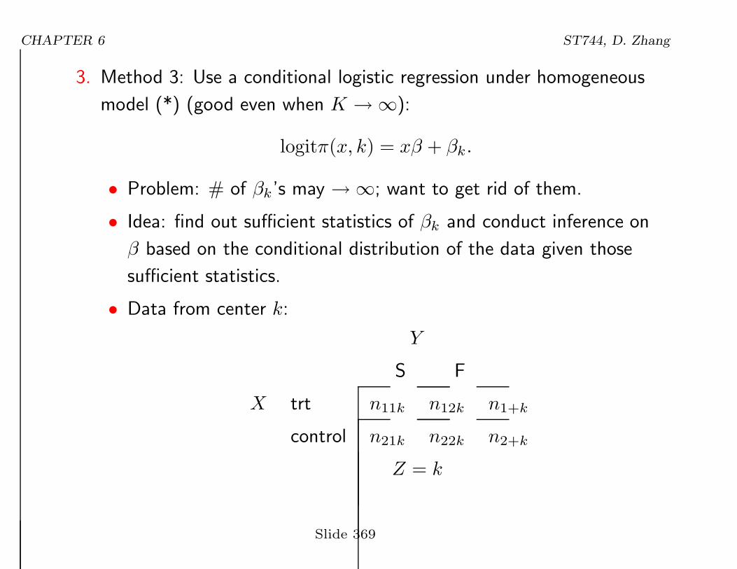
3. Method 3: Use a conditional logistic regression under homogeneous
model (*) (good even when K →∞):
logitπ(x, k) = xβ + βk.
• Problem: # of βk’s may →∞; want to get rid of them.
• Idea: find out sufficient statistics of βk and conduct inference on
β based on the conditional distribution of the data given those
sufficient statistics.
• Data from center k:
Y
S F
X trt n11k n12k n1+k
control n21k n22k n2+k
Z = k
Slide 369
CHAPTER 6 ST744, D. Zhang
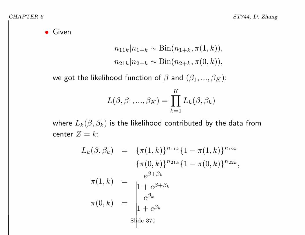
• Given
n11k|n1+k ∼ Bin(n1+k, π(1, k)),
n21k|n2+k ∼ Bin(n2+k, π(0, k)),
we got the likelihood function of β and (β1, ..., βK):
L(β, β1, ..., βK) =K∏
k=1
Lk(β, βk)
where Lk(β, βk) is the likelihood contributed by the data from
center Z = k:
Lk(β, βk) = {π(1, k)}n11k{1− π(1, k)}n12k
{π(0, k)}n21k{1− π(0, k)}n22k ,
π(1, k) =eβ+βk
1 + eβ+βk
π(0, k) =eβk
1 + eβk
Slide 370
CHAPTER 6 ST744, D. Zhang
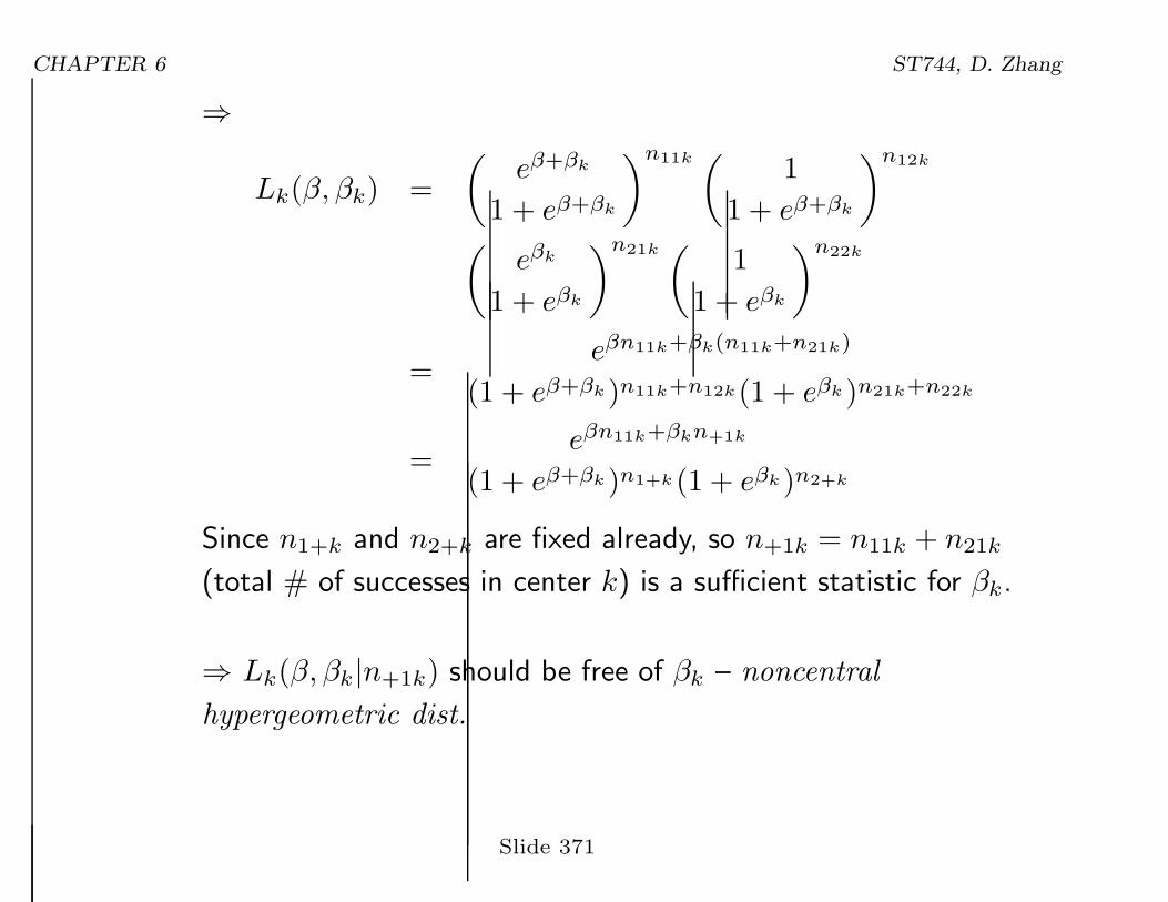
⇒
Lk(β, βk) =
(eβ+βk
1 + eβ+βk
)n11k ( 1
1 + eβ+βk
)n12k
(eβk
1 + eβk
)n21k ( 1
1 + eβk
)n22k
=eβn11k+βk(n11k+n21k)
(1 + eβ+βk)n11k+n12k(1 + eβk)n21k+n22k
=eβn11k+βkn+1k
(1 + eβ+βk)n1+k(1 + eβk)n2+k
Since n1+k and n2+k are fixed already, so n+1k = n11k + n21k
(total # of successes in center k) is a sufficient statistic for βk.
⇒ Lk(β, βk|n+1k) should be free of βk – noncentral
hypergeometric dist.
Slide 371
CHAPTER 6 ST744, D. Zhang
• The conditional logistic inference (on β) is based on the
conditional likelihood:
Lc(β|{n+1k}) =K∏
k=1
Lk(β, βk|n+1k),
which only has one parameter β no matter how large K is!
Treat this as a regular likelihood function, we can estimate β by
maximizing Lc(β|{n+1k}). We can also conduct the Wald, score
and LRT for testing H0 : β = 0.
Slide 372
CHAPTER 6 ST744, D. Zhang
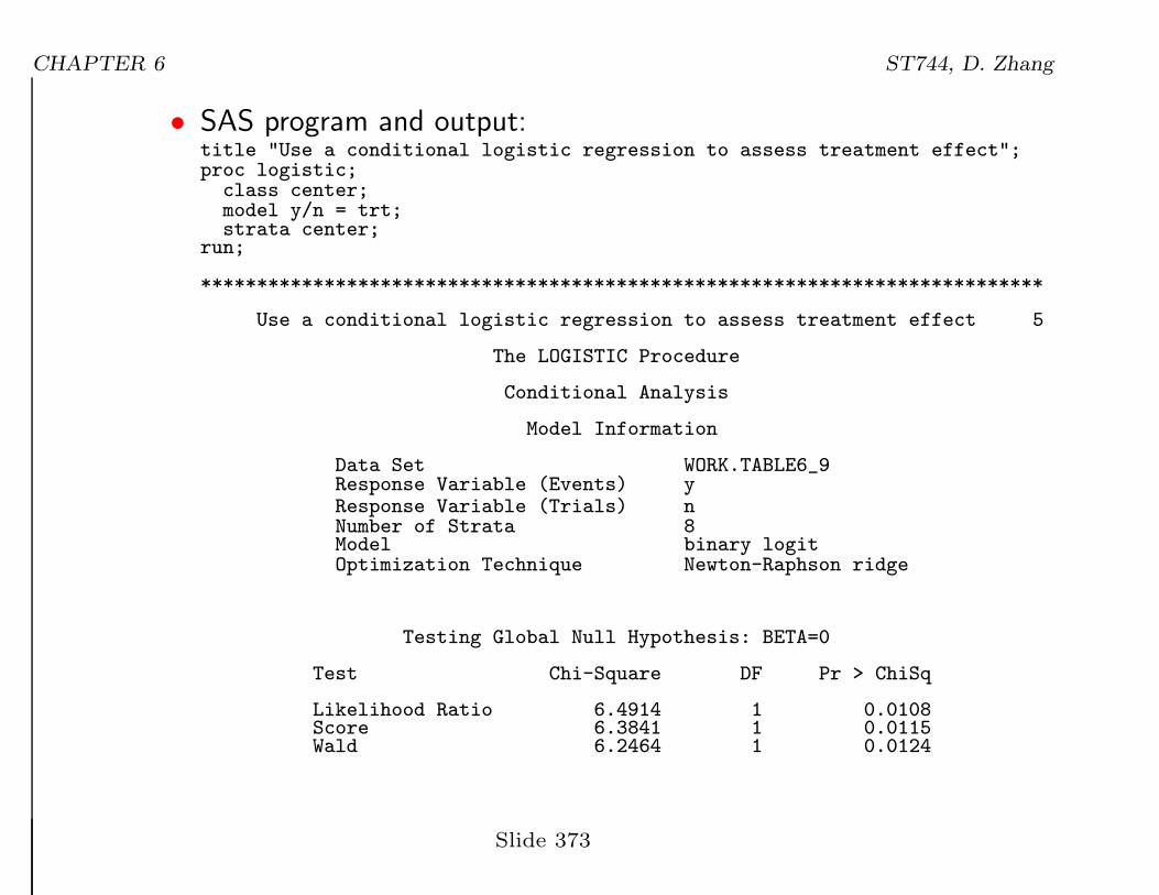
• SAS program and output:title "Use a conditional logistic regression to assess treatment effect";proc logistic;
class center;model y/n = trt;strata center;
run;
***************************************************************************
Use a conditional logistic regression to assess treatment effect 5
The LOGISTIC Procedure
Conditional Analysis
Model Information
Data Set WORK.TABLE6_9Response Variable (Events) yResponse Variable (Trials) nNumber of Strata 8Model binary logitOptimization Technique Newton-Raphson ridge
Testing Global Null Hypothesis: BETA=0
Test Chi-Square DF Pr > ChiSq
Likelihood Ratio 6.4914 1 0.0108Score 6.3841 1 0.0115Wald 6.2464 1 0.0124
Slide 373
CHAPTER 6 ST744, D. Zhang
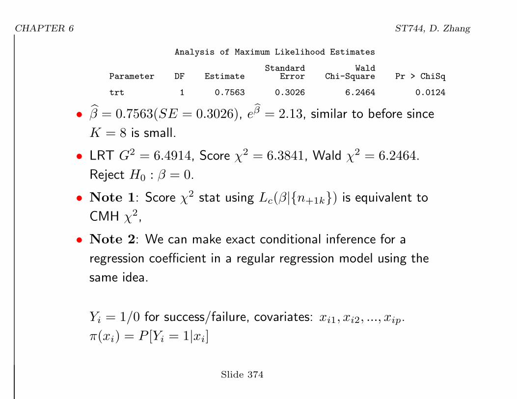
Analysis of Maximum Likelihood Estimates
Standard WaldParameter DF Estimate Error Chi-Square Pr > ChiSq
trt 1 0.7563 0.3026 6.2464 0.0124
• β = 0.7563(SE = 0.3026), ebβ = 2.13, similar to before since
K = 8 is small.
• LRT G2 = 6.4914, Score χ2 = 6.3841, Wald χ2 = 6.2464.
Reject H0 : β = 0.
• Note 1: Score χ2 stat using Lc(β|{n+1k}) is equivalent to
CMH χ2,
• Note 2: We can make exact conditional inference for a
regression coefficient in a regular regression model using the
same idea.
Yi = 1/0 for success/failure, covariates: xi1, xi2, ..., xip.
π(xi) = P [Yi = 1|xi]
Slide 374
CHAPTER 6 ST744, D. Zhang
Model:
logit{π(xi)} = β1xi1 + β2xi2 + · · ·+ βpxip
We can find out suff. stat. for each βk, denoted by Tk. Suppose
we would like to make exact conditional inference on, βp, say,
then the exact inference can be based on
f(y1, y2, ..., yn|T1, T2, ..., Tp−1) = L(βp).
For exact test of H0 : βp = 0, the cond. dist. of data
(Y1, Y2, ..., Yn) given T1, T2, ..., Tp−1 is completely known. We
can do exact score test based on L(βp).
We can also construct an exact CI for βp based on L(βp).
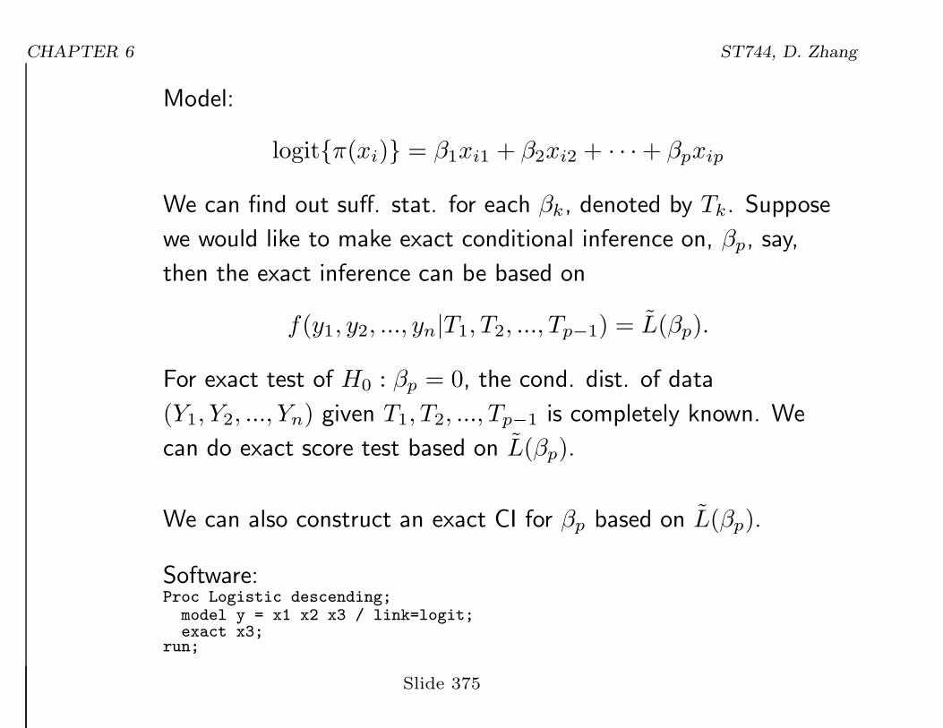
Software:Proc Logistic descending;
model y = x1 x2 x3 / link=logit;exact x3;
run;
Slide 375
CHAPTER 6 ST744, D. Zhang
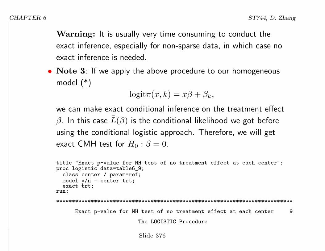
Warning: It is usually very time consuming to conduct the
exact inference, especially for non-sparse data, in which case no
exact inference is needed.
• Note 3: If we apply the above procedure to our homogeneous
model (*)
logitπ(x, k) = xβ + βk,
we can make exact conditional inference on the treatment effect
β. In this case L(β) is the conditional likelihood we got before
using the conditional logistic approach. Therefore, we will get
exact CMH test for H0 : β = 0.
title "Exact p-value for MH test of no treatment effect at each center";proc logistic data=table6_9;
class center / param=ref;model y/n = center trt;exact trt;
run;
***************************************************************************
Exact p-value for MH test of no treatment effect at each center 9
The LOGISTIC Procedure
Slide 376
CHAPTER 6 ST744, D. Zhang
Analysis of Maximum Likelihood Estimates
Standard WaldParameter DF Estimate Error Chi-Square Pr > ChiSq
Intercept 1 0.8859 0.6755 1.7201 0.1897center 1 1 -2.2079 0.7195 9.4166 0.0022center 2 1 -0.1525 0.7381 0.0427 0.8363center 3 1 -1.0550 0.7457 2.0015 0.1571center 4 1 -3.6264 0.9071 15.9813 <.0001center 5 1 -2.7278 0.8184 11.1104 0.0009center 6 1 -4.3548 1.2293 12.5499 0.0004center 7 1 -3.0056 1.0200 8.6836 0.0032trt 1 0.7769 0.3067 6.4174 0.0113
--- p-Value ---Effect Test Statistic Exact Mid
trt Score 6.3841 0.0134 0.0110Probability 0.00469 0.0134 0.0110
We can see that 6.3841 is the CMH χ2, which is the score stat.
based on L(β) (row 1). We can also conduct Fisher exact test
on H0 : β = 0 using table prob. (row 2).
Slide 377
CHAPTER 6 ST744, D. Zhang
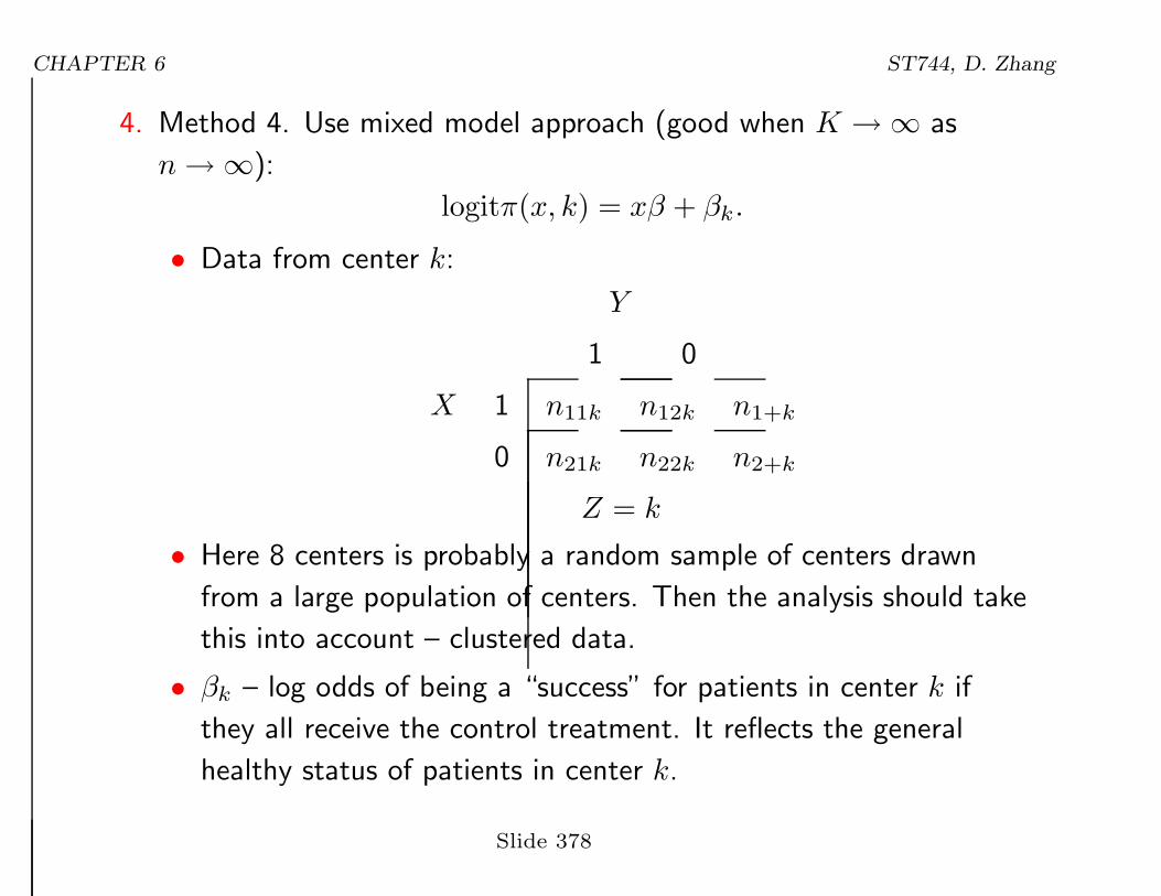
4. Method 4. Use mixed model approach (good when K →∞ as
n→∞):
logitπ(x, k) = xβ + βk.
• Data from center k:
Y
1 0
X 1 n11k n12k n1+k
0 n21k n22k n2+k
Z = k
• Here 8 centers is probably a random sample of centers drawn
from a large population of centers. Then the analysis should take
this into account – clustered data.
• βk – log odds of being a “success” for patients in center k if
they all receive the control treatment. It reflects the general
healthy status of patients in center k.
Slide 378
CHAPTER 6 ST744, D. Zhang
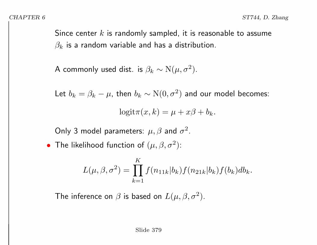
Since center k is randomly sampled, it is reasonable to assume
βk is a random variable and has a distribution.
A commonly used dist. is βk ∼ N(µ, σ2).
Let bk = βk − µ, then bk ∼ N(0, σ2) and our model becomes:
logitπ(x, k) = µ+ xβ + bk.
Only 3 model parameters: µ, β and σ2.
• The likelihood function of (µ, β, σ2):
L(µ, β, σ2) =K∏
k=1
f(n11k|bk)f(n21k|bk)f(bk)dbk.
The inference on β is based on L(µ, β, σ2).
Slide 379
CHAPTER 6 ST744, D. Zhang
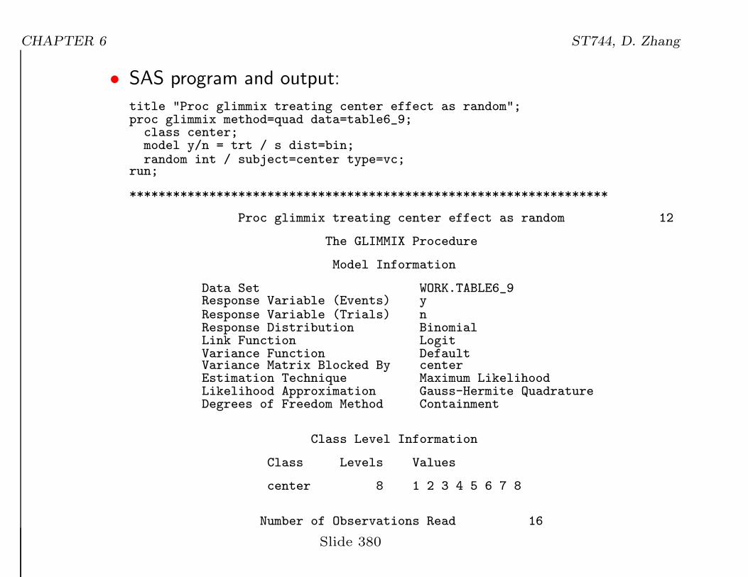
• SAS program and output:
title "Proc glimmix treating center effect as random";proc glimmix method=quad data=table6_9;
class center;model y/n = trt / s dist=bin;random int / subject=center type=vc;
run;
******************************************************************
Proc glimmix treating center effect as random 12
The GLIMMIX Procedure
Model Information
Data Set WORK.TABLE6_9Response Variable (Events) yResponse Variable (Trials) nResponse Distribution BinomialLink Function LogitVariance Function DefaultVariance Matrix Blocked By centerEstimation Technique Maximum LikelihoodLikelihood Approximation Gauss-Hermite QuadratureDegrees of Freedom Method Containment
Class Level Information
Class Levels Values
center 8 1 2 3 4 5 6 7 8
Number of Observations Read 16
Slide 380
CHAPTER 6 ST744, D. Zhang
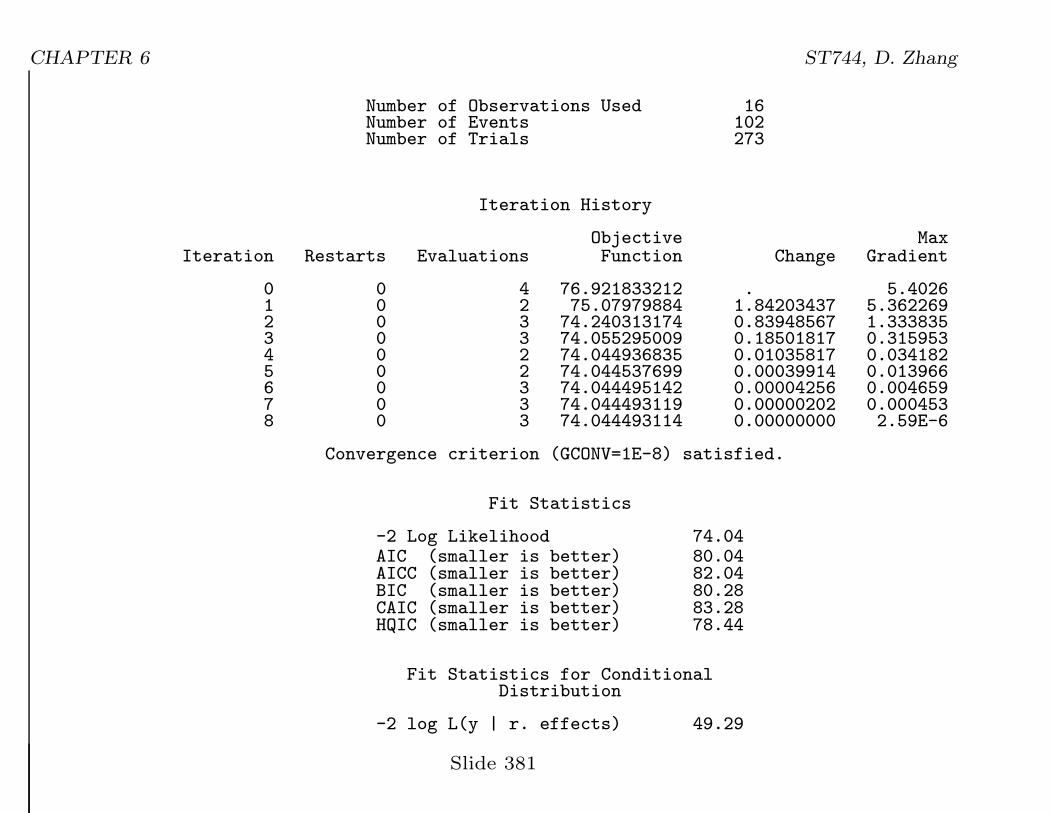
Number of Observations Used 16Number of Events 102Number of Trials 273
Iteration History
Objective MaxIteration Restarts Evaluations Function Change Gradient
0 0 4 76.921833212 . 5.40261 0 2 75.07979884 1.84203437 5.3622692 0 3 74.240313174 0.83948567 1.3338353 0 3 74.055295009 0.18501817 0.3159534 0 2 74.044936835 0.01035817 0.0341825 0 2 74.044537699 0.00039914 0.0139666 0 3 74.044495142 0.00004256 0.0046597 0 3 74.044493119 0.00000202 0.0004538 0 3 74.044493114 0.00000000 2.59E-6
Convergence criterion (GCONV=1E-8) satisfied.
Fit Statistics
-2 Log Likelihood 74.04AIC (smaller is better) 80.04AICC (smaller is better) 82.04BIC (smaller is better) 80.28CAIC (smaller is better) 83.28HQIC (smaller is better) 78.44
Fit Statistics for ConditionalDistribution
-2 log L(y | r. effects) 49.29
Slide 381
CHAPTER 6 ST744, D. Zhang
Pearson Chi-Square 8.37Pearson Chi-Square / DF 0.52
Covariance Parameter Estimates
StandardCov Parm Subject Estimate Error
Intercept center 1.9591 1.1903
Solutions for Fixed Effects
StandardEffect Estimate Error DF t Value Pr > |t|
Intercept -1.1974 0.5561 7 -2.15 0.0683trt 0.7385 0.3004 7 2.46 0.0436
From the output, we see µ = −1.1974
β = 0.7385(SE = 0.3004), ebβ = 2.1.
σ2 = 1.9591, variation in log odds of “success” among centers.
Huge variation.
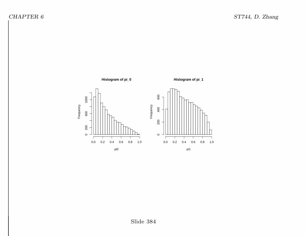
• Since the success prob. for patients receiving control at center k
is
π0k = π(0, k) =
eµ+bk
1 + eµ+bk
Slide 382

CHAPTER 6 ST744, D. Zhang
and the success prob. for patients receiving treatment at center
k is
π1k = π(1, k) =
eµ+β+bk
1 + eµ+β+bk,
we can generate a random sample {bk}’s to get a feeling on the
distributions of π0k and π1
k
π0 = E(π0k) = 0.29, π1 = E(π1
k) = 0.42 ⇒ θXY = 1.77.R function:postscript(file="cream-prob.ps", horizontal = F)par(mfrow=c(1,2), pty="s")
b <- rnorm(10000, 0, sqrt(1.9591))expeta0 <- exp(-1.1974 + b)expeta1 <- exp(-1.1974 + 0.7385 + b)
pi0 <- expeta0/(1+expeta0)pi1 <- expeta1/(1+expeta1)
mean0 <- mean(pi0)mean1 <- mean(pi1)
hist(pi0, main="Histogram of pi_0")hist(pi1, main="Histogram of pi_1")dev.off()
Slide 383
CHAPTER 6 ST744, D. Zhang
Histogram of pi_0
pi0
Fre
quen
cy
0.0 0.2 0.4 0.6 0.8 1.0
020
060
010
00
Histogram of pi_1
pi1F
requ
ency
0.0 0.2 0.4 0.6 0.8 1.0
020
040
060
0
Slide 384
CHAPTER 6 ST744, D. Zhang
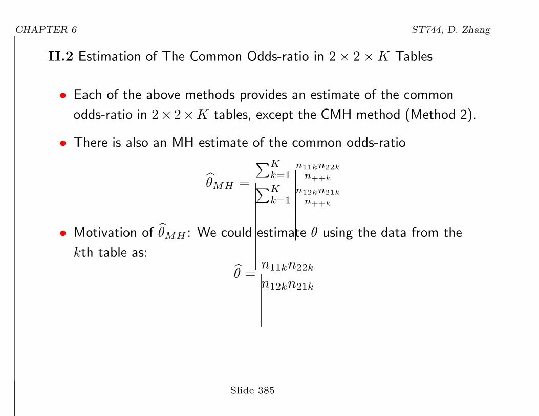
II.2 Estimation of The Common Odds-ratio in 2× 2×K Tables
• Each of the above methods provides an estimate of the common
odds-ratio in 2× 2×K tables, except the CMH method (Method 2).
• There is also an MH estimate of the common odds-ratio
θMH =
∑Kk=1
n11kn22k
n++k∑Kk=1
n12kn21k
n++k
• Motivation of θMH : We could estimate θ using the data from the
kth table as:
θ =n11kn22k
n12kn21k
Slide 385
CHAPTER 6 ST744, D. Zhang
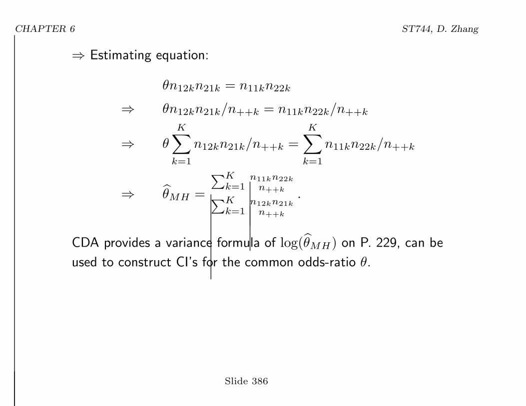
⇒ Estimating equation:
θn12kn21k = n11kn22k
⇒ θn12kn21k/n++k = n11kn22k/n++k
⇒ θ
K∑
k=1
n12kn21k/n++k =
K∑
k=1
n11kn22k/n++k
⇒ θMH =
∑Kk=1
n11kn22k
n++k∑Kk=1
n12kn21k
n++k
.
CDA provides a variance formula of log(θMH) on P. 229, can be
used to construct CI’s for the common odds-ratio θ.
Slide 386
CHAPTER 6 ST744, D. Zhang
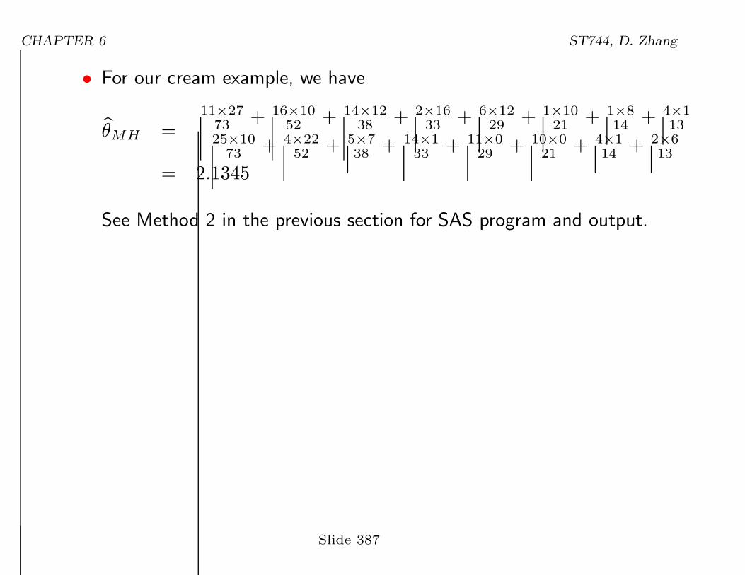
• For our cream example, we have
θMH =11×27
73 + 16×1052 + 14×12
38 + 2×1633 + 6×12
29 + 1×10²¹ + 1×8
14 + 4×113
25×1073 + 4×22
52 + 5×738 + 14×1
33 + 11×029 + 10×0
21 + 4×114 + 2×6
13
= 2.1345
See Method 2 in the previous section for SAS program and output.
Slide 387

CHAPTER 6 ST744, D. Zhang
III Summarizing Predictive Power, Classification Tables and ROC
Curves (P. 223)
• Suppose we have binary response Yi = 1/0 (success/failure), xi a
vector of covariates.
π(xi) = P [Yi = 1|xi]
logit{π(xi)} = xTi β
After we fit the model, we got β ⇒ we got πi as
πi =exT
ibβ
1 + exTi
bβ.
• Choose a known value π0 (e.g., π0 = 0.5), and conduct prediction
Yi as
Yi =
1 if πi > π0
0 otherwise
Slide 388
CHAPTER 6 ST744, D. Zhang
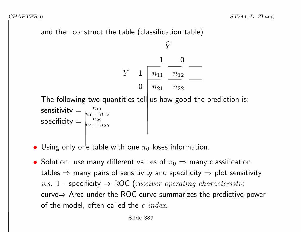
and then construct the table (classification table)
Y
1 0
Y 1 n11 n12
0 n21 n22
The following two quantities tell us how good the prediction is:
sensitivity = n11
n11+n12
specificity = n22
n21+n22
• Using only one table with one π0 loses information.
• Solution: use many different values of π0 ⇒ many classification
tables ⇒ many pairs of sensitivity and specificity ⇒ plot sensitivity
v.s. 1− specificity ⇒ ROC (receiver operating characteristic
curve⇒ Area under the ROC curve summarizes the predictive power
of the model, often called the c-index.
Slide 389
CHAPTER 6 ST744, D. Zhang
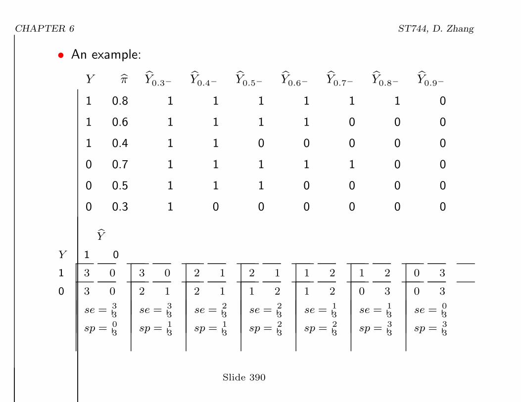
• An example:
Y bπ bY0.3−bY0.4−
bY0.5−bY0.6−
bY0.7−bY0.8−
bY0.9−
1 0.8 1 1 1 1 1 1 0
1 0.6 1 1 1 1 0 0 0
1 0.4 1 1 0 0 0 0 0
0 0.7 1 1 1 1 1 0 0
0 0.5 1 1 1 0 0 0 0
0 0.3 1 0 0 0 0 0 0
bY
Y 1 0
1 3 0
0 3 0
se =3
3
sp =0
3
3 0
2 1
se =3
3
sp =1
3
2 1
2 1
se =2
3
sp =1
3
2 1
1 2
se =2
3
sp =2
3
1 2
1 2
se =1
3
sp =2
3
1 2
0 3
se =1
3
sp =3
3
0 3
0 3
se =0
3
sp =3
3
Slide 390
CHAPTER 6 ST744, D. Zhang
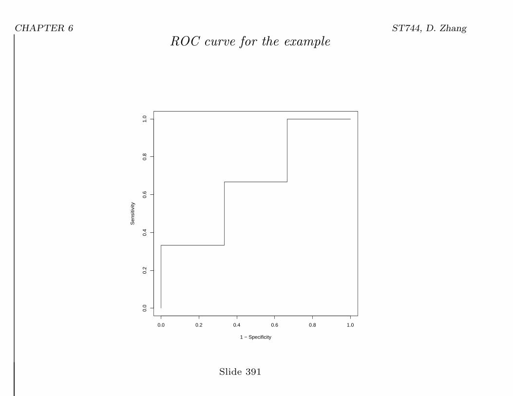
ROC curve for the example
0.0 0.2 0.4 0.6 0.8 1.0
0.0
0.2
0.4
0.6
0.8
1.0
1 − Specificity
Sen
sitiv
ity
Slide 391
CHAPTER 6 ST744, D. Zhang
• The AUC for the above ROC curve:
1− 3
9=
2
3
= proportion of concordant pairs in (Yi, πi) among all pairs with
different outcome Yi.
# of pairs with different outcomes: 3× 3 = 9.
# of concordant pairs: 3 + 2 + 1 = 6.
• If there are ties in πi’s, need to do some adjustment. For example,suppose two πi’ for a Yi = 1 and a Yi = 0 are the same (0.4):
Slide 392
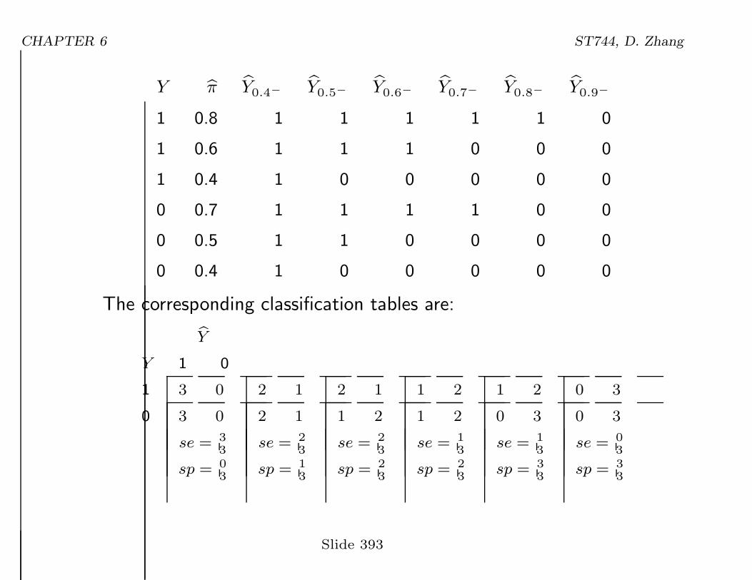
CHAPTER 6 ST744, D. Zhang
Y bπ bY0.4−bY0.5−
bY0.6−bY0.7−
bY0.8−bY0.9−
1 0.8 1 1 1 1 1 0
1 0.6 1 1 1 0 0 0
1 0.4 1 0 0 0 0 0
0 0.7 1 1 1 1 0 0
0 0.5 1 1 0 0 0 0
0 0.4 1 0 0 0 0 0
The corresponding classification tables are:
bY
Y 1 0
1 3 0
0 3 0
se =3
3
sp =0
3
2 1
2 1
se =2
3
sp =1
3
2 1
1 2
se =2
3
sp =2
3
1 2
1 2
se =1
3
sp =2
3
1 2
0 3
se =1
3
sp =3
3
0 3
0 3
se =0
3
sp =3
3
Slide 393
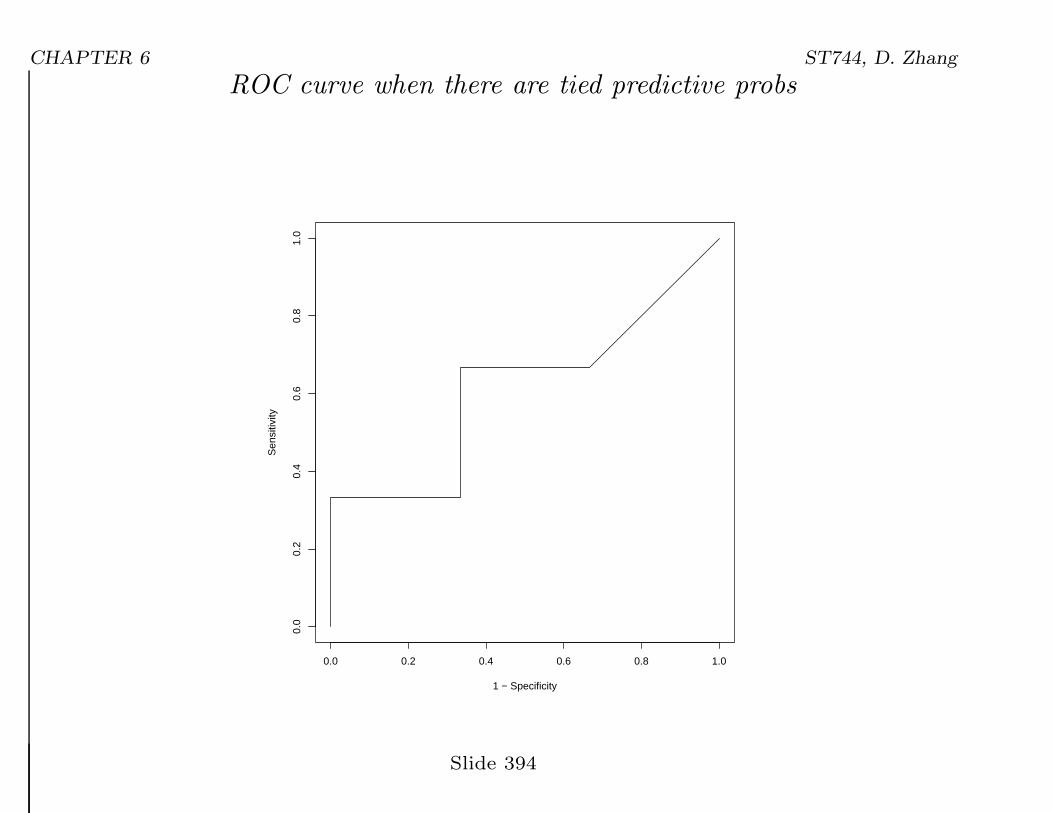
CHAPTER 6 ST744, D. Zhang
ROC curve when there are tied predictive probs
0.0 0.2 0.4 0.6 0.8 1.0
0.0
0.2
0.4
0.6
0.8
1.0
1 − Specificity
Sen
sitiv
ity
Slide 394
CHAPTER 6 ST744, D. Zhang
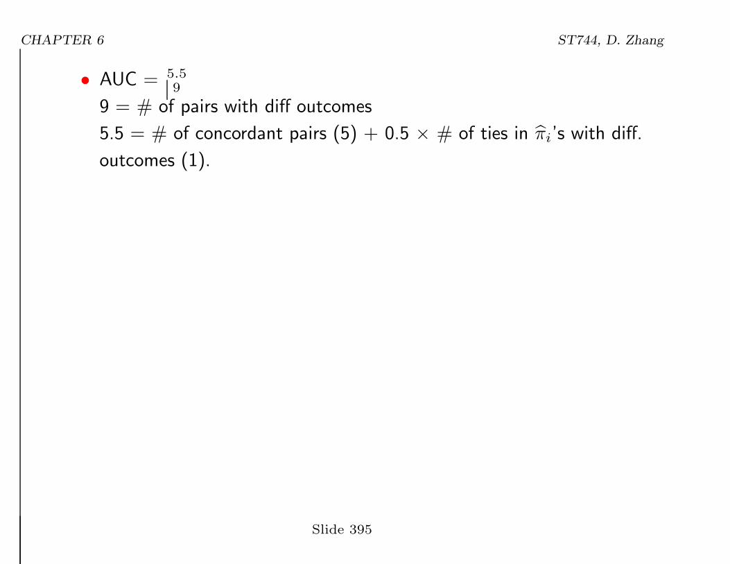
• AUC = 5.59
9 = # of pairs with diff outcomes
5.5 = # of concordant pairs (5) + 0.5 × # of ties in πi’s with diff.
outcomes (1).
Slide 395