5g channel model for bands up to100 ghz2015... · 5g channel model for bands up to100 ghz...
TRANSCRIPT

5G Channel Model for bands up to100 GHz
Contributors:
Aalto UniversityBUPTCMCC
NokiaNTT DOCOMONew York University
Ericsson QualcommHuawei SamsungINTEL University of BristolKT Corporation University of Southern California

Executive Summary
The future mobile communications systems are likely to be very different to those of today with new
service innovations driven by increasing data traffic demand, increasing processing power of smart
devices and new innovative applications. To meet these service demands the telecommunication
industry is converging on a common set of 5G requirements which includes network speeds as high as
10 Gbps, cell edge rate greater than 100 Mbps and latency of less than 1msec. To be able to reach
these 5G requirements the industry is looking at new spectrum bands in the range up to 100 GHz
where there is spectrum availability for wide bandwidth channels.. For the development of the new
5G systems to operate in bands up to 100 GHz there is a need for accurate radio propagation models
for these bands which are not addressed by existing channel models developed for bands below 6
GHz. This white paper presents a preliminary overview of the 5G channel models for bands up to 100
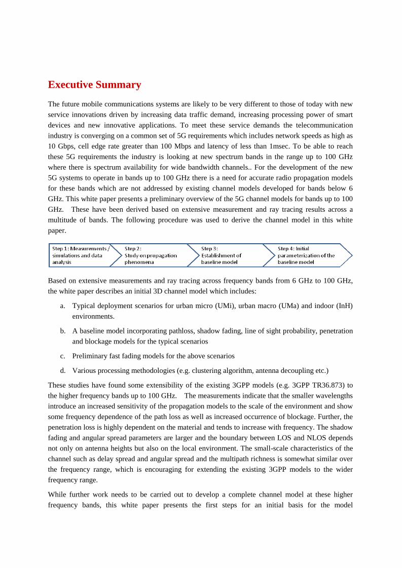
GHz. These have been derived based on extensive measurement and ray tracing results across a
multitude of bands. The following procedure was used to derive the channel model in this white
paper.
Based on extensive measurements and ray tracing across frequency bands from 6 GHz to 100 GHz,
the white paper describes an initial 3D channel model which includes:
a. Typical deployment scenarios for urban micro (UMi), urban macro (UMa) and indoor (InH)
environments.
b. A baseline model incorporating pathloss, shadow fading, line of sight probability, penetration
and blockage models for the typical scenarios
c. Preliminary fast fading models for the above scenarios
d. Various processing methodologies (e.g. clustering algorithm, antenna decoupling etc.)
These studies have found some extensibility of the existing 3GPP models (e.g. 3GPP TR36.873) to
the higher frequency bands up to 100 GHz. The measurements indicate that the smaller wavelengths
introduce an increased sensitivity of the propagation models to the scale of the environment and show
some frequency dependence of the path loss as well as increased occurrence of blockage. Further, the
penetration loss is highly dependent on the material and tends to increase with frequency. The shadow
fading and angular spread parameters are larger and the boundary between LOS and NLOS depends
not only on antenna heights but also on the local environment. The small-scale characteristics of the
channel such as delay spread and angular spread and the multipath richness is somewhat similar over
the frequency range, which is encouraging for extending the existing 3GPP models to the wider
frequency range.
While further work needs to be carried out to develop a complete channel model at these higher
frequency bands, this white paper presents the first steps for an initial basis for the model

development.

Contents
Executive Summary ............................................................................................................................................. 3
1 Introduction.................................................................................................................................................. 6
2 Requirements for new channel model ........................................................................................................ 7
3 Typical Deployment Scenarios.................................................................................................................... 8
3.1 Urban Micro (UMi) Street Canyon and Open Square with outdoor to outdoor (O2O) and outdoor to
indoor (O2I) ....................................................................................................................................................... 9
3.2 Indoor (InH)– Open and closed Office, Shopping Malls ....................................................................... 9
3.3 Urban Macro (UMa) with O2O and O2I ............................................................................................. 10
4 Characteristics of the Channel in 6 GHz-100 GHz ................................................................................. 10
4.1 UMi Channel Characteristics............................................................................................................... 11
4.2 UMa Channel Characteristics .............................................................................................................. 11
4.3 InH Channel Characteristics ................................................................................................................ 11
4.4 Penetration Loss in all Environments .................................................................................................. 12
4.4.1 Outdoor to indoor channel characteristics ....................................................................................... 12
4.4.2 Inside buildings ............................................................................................................................... 14
4.5 Blockage in all Environments.............................................................................................................. 15
5 Channel Modeling Considerations ........................................................................................................... 16
6 Pathloss, Shadow Fading, LoS and Blockage Modeling ......................................................................... 20
6.1 LOS probability ................................................................................................................................... 20
6.2 Path loss models .................................................................................................................................. 23
6.3 Building penetration loss modelling .................................................................................................... 26
6.4 Blockage models.................................................................................................................................. 27
7 Fast Fading Modeling ................................................................................................................................ 28
7.1 UMi...................................................................................................................................................... 28
7.2 UMa..................................................................................................................................................... 30
7.3 InH....................................................................................................................................................... 31
7.4 O2I channel modelling ........................................................................................................................ 31
References ........................................................................................................................................................... 52
List of Acronyms ................................................................................................................................................ 55

1 Introduction
Next generation 5G cellular systems will encompass frequencies from around 500 MHz all the way to
around 100 GHz. For the development of the new 5G systems to operate in bands above 6 GHz,
there is a need for accurate radio propagation models for these bands which are not fully modelled by
existing channel models below 6 GHz.. Previous generations of channel models were designed and
evaluated for operation at frequencies only as high as 6 GHz. One important example is the recently
developed 3D-urban micro (UMi) and 3D-urban macro (UMa) channel models for LTE [3GPP
TR36.873]. The 3GPP 3D channel model provides additional flexibility for the elevation dimension,
thereby allowing modeling two dimensional antenna systems, such as those that are expected in next
generation system deployments. It is important for future system design to develop a new channel
model that will be validated for operation at higher frequencies (e.g., up to 100 GHz) and that will
allow accurate performance evaluation of possible future technical specifications for these bands over
a representative set of possible environments and scenarios of interest. Furthermore, the new models
should be consistent with the models below 6 GHz. In some cases, the requirements may call for
deviations from the modelling parameters or methodology of the existing models, but these deviations
should be kept to a bare minimum and only introduced when necessary for supporting the 5G
simulation use cases.
There are many existing and ongoing campaign efforts worldwide targeting 5G channel
measurements and modeling. They include METIS202 [METIS 2015], COST2100/COST[COST],
IC1004 [IC], ETSI mmWave SIG [ETSI 2015], 5G mmWave Channel Model Alliance [NIST],
MiWEBA [MiWEBA 2014], mmMagic [mmMagic], and NYU WIRELESS [Rappaport 2015,
MacCartney 2015, Rappaport 2013, Samimi 2015]. METIS2020, for instance, has focused on 5G
technologies and has contributed extensive studies in terms of channel modelling. Their target
requirements include a wide range of frequency bands (up to 86 GHz), very large bandwidths
(hundreds of MHz), fully three dimensional and accurate polarization modelling, spherical wave
modelling, and high spatial resolution. The METIS channel models consist of a map-based model,
stochastic model, and a hybrid model which can meet requirement of flexibility and scalability. The
COST2100 channel model is a geometry-based stochastic channel model (GSCM) that can reproduce
the stochastic properties of multiple-input/multiple output (MIMO) channels over time, frequency,
and space. On the other hand, the 5G mmWave Channel Model Alliance is newly established and will
establish guidelines for measurement calibration and methodology, modeling methodology, as well as
parameterization in various environments and a database for channel measurement campaigns. NYU
WIRELESS has conducted and published extensive urban propagation measurements at 28, 38 and 73
GHz for both outdoor and indoor channels, and has created large-scale and small-scale channel
models and concepts of spatial lobes to model multiple multipath time clusters that are seen to arrive
in particular directions [Rappaport 2013,Rappaport 2015, Samimi GCW2015, MacCartney 2015,
Samimi EUCAP2016 ].
In this white paper, we present a brief overview of the channel properties for bands up to 100 GHz
based on extensive measurement and ray tracing results across a multitude of bands. In addition we

present a preliminary set of channel parameters suitable for 5G simulations that are capable of
capturing the main properties and trends.
2 Requirements for new channel model
The requirements of the new channel model that will support 5G operation across frequency bands up
to 100 GHz are outlined below:
1. The new channel model should preferably be based on the existing 3GPP 3D channel model
[3GPP TR36.873] but with extensions to cater for additional 5G modeling requirements and
scenarios, for example:
a.Antenna arrays, especially at higher-frequency millimeter-wave bands, will very likely
be 2D and dual-polarized both at the access point (AP) and the user equipment (UE)
and will hence need properly-modeled azimuth and elevation angles of departure and
arrival of multipath components.
b.Individual antenna elements will have antenna radiation patterns in azimuth and
elevation and may require separate modeling for directional performance gains.
Furthermore, polarization properties of the multipath components need to be
accurately accounted for in the model.
2. The new channel model must accommodate a wide frequency range up to 100 GHz. The
joint propagation characteristics over different frequency bands will need to be evaluated for
multi-band operation, e.g., low-band and high-band carrier aggregation configurations.
3. The new channel model must support large channel bandwidths (up to 2GHz), where:
a.The individual channel bandwidths may be in the range of 100 MHz to 2 GHz and may
support carrier aggregation.
b.The operating channels may be spread across an assigned range of several GHz
4. The new channel model must support a range of large antenna arrays, in particular:
a.Some large antenna arrays will have very high directivity with angular resolution of the
channel down to around 1.0 degree.
b.5G will consist of different array types, e.g., linear, planar, cylindrical and spherical
arrays, with arbitrary polarization.
c.The array manifold vector can change significantly when the bandwidth is large relative
to the carrier frequency. As such, the wideband array manifold assumption is not
valid and new modeling techniques may be required. It may be preferable, for
example, to model arrival/departure angles with delays across the array and follow a
spherical wave assumption instead of the usual plane wave assumption.
5. The new channel model must accommodate mobility, in particular:

a.The channel model structure should be suitable for mobility up to 350 km/hr.
b.The channel model structure should be suitable for small-scale mobility and rotation of
both ends of the link in order to support scenarios such as device to device (D2D) or
vehicle to vehicle (V2V).
6. The new channel model must ensure spatial/temporal/frequency consistency, in particular:
a.The model should provide spatial/temporal/frequency consistencies which may be
characterized, for example, via spatial consistence, inter-site correlation, and
correlation among frequency bands.
b.The model should also ensure that the channel states, such as Line Of Sight
(LOS)/non-LOS (NLOS) for outdoor/indoor locations, the second order statistics of
the channel, and the channel realizations change smoothly as a function of time,
antenna position, and/or frequency in all propagation scenarios.
c.The spatial/temporal/frequency consistencies should be supported for simulations
where the channel consistency impacts the results (e.g. massive MIMO, mobility and
beam tracking, etc.). Such support could possibly be optional for simpler studies.
7. The new channel model must be of practical computational complexity, in particular:
a.The model should be suitable for implementation in single-link simulation tools and in
multi-cell, multi-link radio network simulation tools. Computational complexity and
memory requirements should not be excessive. The 3GPP 3D channel model [3GPP
TR36.873] is seen, for instance, as a sufficiently accurate model for its purposes, with
an acceptable level of complexity. Accuracy may be provided by including additional
modeling details with reasonable complexity to support the greater channel
bandwidths, and spatial and temporal resolutions and spatial/temporal/frequency
consistency, required for millimeter-wave modeling.
b.The introduction of a new modeling methodology (e.g. Map based model) may
significantly complicate the channel generation mechanism and thus substantially
increase the implementation complexity of the system-level simulator. Furthermore,
if one applies a completely different modeling methodology for frequencies above 6
GHz, it would be difficult to have meaningful comparative system evaluations for
bands up to 100 GHz.
3 Typical Deployment Scenarios
The traditional modeling scenarios (UMa, UMi and indoor hotspot (InH)) have previously been
considered in 3GPP for modeling of the radio propagation in bands below about 6 GHz. The new
channel model discussed in this paper is for a selective set of 5G scenarios and encompasses the
following cases:

3.1 Urban Micro (UMi) Street Canyon and Open Square with outdoor to outdoor (O2O)and outdoor to indoor (O2I)
Figure 1. UMi Street Canyon
Figure 2. UMi Open Square
A typical UMi scenario is shown for street canyon and open square in Figure 1 and Figure 2,
respectively. The cell radii for UMi is typically less than 100 m and the access points (APs)
are mounted below rooftops (e.g., 3-20 m). The UEs are deployed outdoor at ground level or
indoor at all floors.
3.2 Indoor (InH)– Open and closed Office, Shopping Malls
The indoor scenario includes open and closed offices, corridors within offices and shopping
malls as examples. The typical office environment has open cubicle areas, walled offices,
open areas, corridors, etc., where the partition walls are composed of a variety of materials
like sheetrock, poured concrete, glass, cinder block, etc. For the office environment, the APs
are mounted at a height of 2-3 m either on the ceilings or walls. The shopping malls are
generally 2-5 stories high and often include an open area (“atrium”). In the shopping-mall
environment, the APs are mounted at a height of approximately 3 m on the walls or ceilings
of the corridors and shops. The density of the APs may range from one per floor to one per
room, depending on the frequency band and output power The typical indoor office scenario
and shopping malls are shown in Figure 3 and Figure 4, respectively.

Figure 3. Typical Indoor Office
Figure 4. Indoor Shopping Malls
3.3 Urban Macro (UMa) with O2O and O2I
Figure 5. UMa Deployment
The cell radii for UMa is typically above 200 m and the APs are mounted on or above
rooftops (e.g. 25-35 m), an example of which is shown in Figure 5. The UEs are deployed
both outdoor at ground level and indoor at all floors.
4 Characteristics of the Channel in 6 GHz-100 GHz
Measurements over a wide range of frequencies have been performed by the co-signatories of this
white paper. However, due to the more challenging link budgets at higher frequencies there are few

measurements at larger distances, e.g. beyond 200-300 m in UMi or in severely shadowed regions at
shorter distances. In UMa measurements were able to be made at least in the Aalborg location at
distances up to 1.24 km. An overview of the measurement and ray-tracing campaigns can be found
in the Appendix. In the following sections we outline the main observations per scenario with some
comparisons to the existing 3GPP models for below 6 GHz (e.g. [3GPP TR36.873]).
4.1 UMi Channel Characteristics
The LOS path loss in the bands of interest appears to follow Friis’ free space path loss model quitewell. Just as in lower bands, a higher path loss slope (or path loss exponent) is observed in NLOS
conditions. The shadow fading in the measurements appears to be similar to lower frequency bands,
while ray-tracing results show a much higher shadow fading (>10 dB) than measurements, due to
the larger dynamic range allowed in some ray tracing experiments.
In NLOS conditions at frequencies below 6.0 GHz, the RMS delay spread is typically modelled at
around 50-500 ns, the RMS azimuth angle spread of departure (from the AP) at around 10-30°, and
the RMS azimuth angle spread of arrival (at the UE) at around 50-80° [3GPP TR36.873]. There are
measurements of the delay spread above 6 GHz which indicate somewhat smaller ranges as the
frequency increases, and some measurements show the millimeter wave omnidirectional channel to be
highly directional in nature.
4.2 UMa Channel Characteristics
Similar to the UMi scenario, the LOS path loss behaves quite similar to free space path loss as
expected. For the NLOS path loss, the trends over frequency appear somewhat inconclusive across a
wide range of frequencies. The rate at which the loss increases with frequency does not appear to be
linear, as the rate is higher in the lower part of the spectrum. This could possibly be due to diffraction,
which is frequency dependent, being a more dominating propagation mechanism at the lower
frequencies. At higher frequencies reflections and scattering may be more predominant. Alternatively,
the trends could be biased by the lower dynamic range in the measurements at the higher frequencies.
More measurements are needed to understand the UMa channel.
From preliminary ray-tracing studies, the channel spreads in delay and angle appear to be weakly
dependent on the frequency and are generally 2-5 times smaller than in [3GPP TR36.873].
The cross-polar scattering in the ray-tracing results tends to increase (lower XPR) with increasing
frequency due to diffuse scattering.
4.3 InH Channel Characteristics
In LOS conditions, multiple reflections from walls, floor, and ceiling give rise to waveguiding.
Measurements in both office and shopping mall scenarios show that path loss exponents, based on a 1
m free space reference distance, are typically below 2, leading to more favorable path loss than
predicted by Friis’ free space loss formula. The strength of the waveguiding effect is variable and thepath loss exponent appears to increase very slightly with increasing frequency, possibly due to the
relation between the wavelength and surface roughness.
Measurements of the small scale channel properties such as angular spread and delay spread have
shown remarkable similarities between channels over a very wide frequency range. It appears as if the
main multipath components are present at all frequencies though with some smaller variations in
amplitudes.
Recent work shows that polarization discrimination ranges between 15 and 25 dB for indoor
millimeter wave channels [Karttunen EuCAP2015], with greater polarization discrimination at 73
GHz than at 28 GHz [MacCartney 2015].
4.4 Penetration Loss in all Environments
4.4.1 Outdoor to indoor channel characteristics
In both the UMa and the UMi scenario a significant portion of UEs or devices are expected to be
indoors. These indoor UEs increase the strain on the link budget since additional losses are associated
with the penetration into buildings. The characteristics of the building penetration loss and in
particular its variation over the higher frequency range is therefore of high interest and a number of
recent measurement campaigns have been targeting the material losses and building penetration losses
at higher frequencies [Rodriguez VTC Fall 2014], [Zhao 2013], [Larsson EuCAP 2014]. The current
understanding, based on these measurements is briefly summarized as follows.
Different materials commonly used in building construction have very diverse penetration loss
characteristics. Common glass tends to be relatively transparent with a rather weak increase of loss
with higher frequency due to conductivity losses. "Energy-efficient" glass commonly used in modern
buildings or when renovating older buildings is typically metal-coated for better thermal insulation.
This coating introduces additional losses that can be as high as 40 dB even at lower frequencies.
Materials such as concrete or brick have losses that increase rapidly with frequency. Figure 6
summarizes some recent measurements of material losses. The loss trends with frequency are linear to
a first order of approximation. Variations around the linear trend can be understood from multiple
reflections within the material or between different layers which cause constructive or destructive
interference depending on the frequency and incidence angle.

Figure 6. Measured material penetration losses. Sources: [Rodriguez VTC Fall 2014], [Zhao 2013],
and measurements by Samsung and Nokia.
Figure 7. Effective building penetration loss measurements. The bars indicate variability for a given
building. Sources: [Larsson EuCAP 2014] and measurements by Qualcomm, NTT DOCOMO, and

Ericsson. The solid curves represent two variants of the model described in [Semaan Globecomm
2015], which is one out of several penetration loss models considered in this white paper.
Typical building facades are composed of several materials, e.g. glass, concrete, metal, brick, wood,
etc. Propagation of radio waves into or out of a building will in most cases be a combination of
transmission paths through different materials, i.e. through windows and through the facade between
the windows. The exception could be when very narrow beams are used which only illuminates a
single material or when the indoor node is very close to the external wall. Thus, the effective
penetration loss can behave a bit differently than the single material loss. A number of recent
measurements of the effective penetration loss are summarized in Figure 7. As indicated by the bars
available for some of the measurements, there can be quite some variation even in a single building.
For comparison, two models that attempt to capture the loss characteristics of buildings consisting of
multiple materials are shown. The loss characteristics of each specific material follows the results
shown in Figure 7 quite well which indicates that the results in the material loss measurements and the
effective penetration loss measurements are actually fairly consistent even though the loss values
behave differently.
The majority of the results presented so far have been waves with perpendicular incidence to the
external wall. As the incidence angles become more grazing the losses have been observed to increase
by up to 15-20 dB.
Propagation deeper into the building will also be associated with an additional loss due to internal
walls, furniture etc. This additional loss appears to be rather weakly frequency-dependent but rather
strongly dependent on the interior composition of the building. Observed losses over the 2-60 GHz
range of 0.2-2 dB/m.
4.4.2 Inside buildings
Measurements have been reported for penetration loss for various materials at 2.5, 28, and 60 GHz for
indoor scenarios [Rappaport Book2015] [Rappaport 2013] [And 2002][ Zhao 2013]. For easy
comparisons, walls and drywalls were lumped into a common dataset and different types of clear class
were lumped into a common dataset with normalized penetration loss shown in Figure 8. It was
observed that clear glass has widely varying attenuation (20 dB/cm at 2.5 GHz, 3.5 dB/cm at 28 GHz,
and 11.3 dB/cm at 60 GHz). For mesh glass, penetration was observed to increase as a function of
frequency (24.1 dB/cm at 2.5 GHz and 31.9 dB/cm at 60 GHz), and a similar trend was observed with
whiteboard penetration increasing as frequency increased. At 28 GHz, indoor tinted glass resulted in a
penetration loss 24.5 dB/cm. Walls showed very little attenuation per cm of distance at 28 GHz (less
than 1 dB/cm).

Figure 8. 2.5 GHz, 28 GHz, and 60 GHz normalized material penetration losses from indoor
measurements with common types of glass and walls lumped into common datasets [Rappaport 2013]
[And2002][ Zhao 2013] [Nie 2013].
4.5 Blockage in all Environments
As the radio frequency increases, its propagation behaves more like optical propagation and may
become blocked by intervening objects. Typically, two categories of blockage are considered:
dynamic blockage and geometry-induced blockage. Dynamic blockage is caused by the moving
objects (i.e., cars, people) in the communication environment. The effect is transient additional loss on
the paths that intercept the moving object. Figure 9 shows such an example from 28 GHz
measurement done by Fraunhofer HHI in Berlin. In these experiments, time continuous measurements
were made with the transmitter and receiver on each side of the road that had on-off traffic controlled
by traffic light. Note that the time periods when the traffic light is red is clearly seen in the figure as
periods with little variation as the vehicles are static at that time. When the traffic light is green, the
blocking vehicles move through the transmission path at a rapid pace as is seen in the figure. The
variations seen when the light is red are explained by vehicles turning the corner to pass between the
transmitter and receiver.

Figure 9 Example of dynamic blockage from a measurement snapshot at 28 GHz
Geometry-induced blockage, on the other hand, is a static property of the environment. It is caused by
objects in the map environment that block the signal paths. The propagation channels in
geometry-induced blockage locations are dominated by diffraction and sometimes by diffuse
scattering. The effect is an exceptional additional loss beyond the normal path loss and shadow
fading. Figure 10 illustrates examples of diffraction-dominated and reflection-dominated regions in an
idealized scenario. As compared to shadow fading caused by reflections, diffraction-dominated
shadow fading could have different statistics (e.g., different mean, variance and coherence distance).
Tx
DiffractionReg Reflection-
dominatedReg
LOS region
Figure 10 Example of diffraction-dominated and reflection-dominated regions (idealized scenario)
5 Channel Modeling Considerations
Table 1 summarizes a review of the 3GPP 3D channel model [3GPP TR36.873] capabilities. A plus
sign “+” means that the current 3GPP 3D channel model supports the requirement, or the necessary
changes are very simple. A minus sign “-” means that the current channel model does not support the
requirement. This evaluation is further split into two frequency ranges: below 6 GHz and above 6
GHz. Note that in the table, LSP stands for large-scale parameter.

Table 1. Channel Modeling Considerations
Attribute Requirement Below6 GHz
Above6 GHz
Improvementaddressed in
this whitepaper
Comments
#1 Scenarios Support of newscenarios such asindoor office,stadium, shoppingmall etc.- - Current 3GPPmodel supportsUMi and UMa
0.5 GHz – 100 GHzsupported + - Current 3GPPmodel 2 – 6 GHz#2 FrequencyRange Consistency ofchannel modelparametersbetween differentfrequency bands
- - E.g. shadowing,angle of departure,and in carrieraggregation#3 Bandwidth ~100 MHz BW forbelow 6 GHz,2 GHz BW forabove 6 GHz
+ -
Spatial consistencyof LSPs with fixedBS+ - LSP map (2D or3D)
Spatial consistencyof LSPs witharbitrary Tx / Rxlocations (D2D /V2V)- - Complexity issue(4D or 6D map)
Fair comparison ofdifferent networktopologies- -
Spatial consistencyof SSPs - - Autocorrelation ofSSPsUDN / MUConsistency - - Sharing of objects/ clustersDistributedantennas andextremely largearrays- -
#4 SpatialConsistency
Dynamic channel(smooth evolutionof SSPs and LSPs)- - Tx / Rx / scatterermobilityPossible methods

for modelingvarying DoDs andDoAs are discussedin the AppendixSpherical wave - - Also far fieldsphericalHigh angularresolution down to1 degree- - Realistic PAS?
Accurate modelingof Laplacian PAS - - 20 sinusoidsproblem
#5 LargeArray Support
Very large arraysbeyondconsistencyinterval- -
Dual Doppler + - Not yet done,but should be easyDual angle ofarrival (AoA) + - Not yet done,but should be easyDual AntennaPattern (mobileantenna pattern atboth ends of thelink)+ - Not yet done,but should be easy
Arbitrary UEheight (e.g.different floors)- -
#6Dual-mobilitysupport (D2D,V2V)
Spatially consistentmulti-dimensionalmap- - Complexity issue(4D or 6D map)
#7 LOSProbability
Spatially consistentLOS probability /LOS existence- -
#8 SpecularReflection
? - Important in mmWFrequencydependent pathloss model
+ - #9 Path Loss
Power scaling(directive antennasvs.? -

omnidirectional)Multiple NLOScases ? - Important in mmWLog-normalshadowing + - Shadow fading(SF) parametersneeded for highfrequency
#10Shadowing
Body shadowing - -
#11 Blockage Blockage modelling - -
#12 Clusterdefinition
3GPP 3D cluster isdefined as fixeddelay andLaplacian shapeangular spread.+ - It is notguaranteed thatthe Laplacianshape cluster isvalid for mmW.
#13 Dropconcept (blockstationarity)
APs and UEs aredropped in somemanner (e.g.,hexagonal grid for3GPP)+ - It is not sure if thedrop conceptworks perfectly inmmWave. Also it isnot clear how totest beam tracking,for instance.
#14 AccurateLSPCorrelation
Consistentcorrelation of LSPsis needed.- - The current 3GPPmodel providesdifferent resultdepending on theorder ofcalculation(autocorrelation,cross-correlation)
#15 Numberof Paths
The number ofpaths needs to beaccurate acrossfrequency.+ - The current modelis based on lowfrequencymeasurements.
#16 MovingEnvironment
Cars, people,vegetation etc. - -

#17 DiffusePropagation
Specular vs. diffusepower ratio,modeling of diffusescattering+ - Most mmWmeasurementsreport specularonly despite thefact that diffuseexists
6 Pathloss, Shadow Fading, LoS and Blockage Modeling
6.1 LOS probability
The definition of LOS used in this white paper is discussed in this sub-section together with other
LOS models. The LOS state is determined by a map-based approach, i.e., by considering the
transmitter (AP) and receiver (UE) positions and whether any buildings or walls are blocking the
direct path between the AP and the UE. The impact of objects not represented in the map such as trees,
cars, furniture, etc. is modelled separately using shadowing/blocking terms. An attractive feature of
this LOS definition is that it is frequency independent , as only buildings and walls are considered in
the definition.
The first LOS probability model considered, the d1/d2 model, is the current 3GPP/ITU model [3GPP
TR36.873] [ITU M.2135-1]:
22 //1 11,min)( dddd eed
ddp
, (1)
where d is the 2D distance in meters and d1 and d2 can both be optimized to fit a set of data (or
scenario parameters).
The next LOS probability model considered, the NYU (squared) model, is the one developed by NYU
in [Samimi 2015]:
2
//1 2211,min)(
dddd ee
d
ddp , (2)
where again d1 and d2 can be optimized to fit a given set of data (or scenario parameters).
An investigation into the LOS probability for the UMa environment was conducted using all of the
UMa measured and ray tracing data listed in the appendix. In addition to comparing the two models
considered above with optimized d1 and d2 values, the data was also compared to the current 3GPP
UMa LOS probability model (eqn (1)) for a UE height of 1.5 m with d1=18 and d2=63. A summary
of the results is given in Table 2 and the three models are compared to the data in Figure 11. In
terms of mean squared error (MSE) between the LOS probability from the data and the models, the
NYU (squared) model had the lowest MSE, but the difference was small. Given that the current 3GPP
UMa model was a reasonable match to the data and included support for 3D placement of UEs, it is
recommended that the current 3GPP LOS probability model for UMa be used for frequencies above
6.0 GHz. The 3GPP Uma model specifically is [3GPP TR36.873]:

),(111,18
min)( 63/63/UT
dd hdCeed
dp
, (3)
where hUT is the height of the UE in m and:
mhdgh
mh
hdCUT
UT
UT
UT 2313),(10
13
13,0
),(5.1
, (4)
md
otherwise
ddedg 18,
,0
150/exp)25.1()(
26
, (5)
Note that for indoor users d is replaced by the 2D distance to the outer wall.
Table 2. Comparison of the LOS probability models for the UMa environment
d1 d2 MSE
3GPP UMa 18 63 0.020
d1/d2 model 20 66 0.017
NYU (squared) 20 160 0.015
0 100 200 300 400 500 6000
0.1
0.2
0.3
0.4
0.5
0.6
0.7
0.8
0.9
1
Distance (m)
LOS
pro
babi
lity
Data
3GPP UMa
d1/d2 model
NYU (squared) model
Figure 11. UMa LOS probability for the three models considered.
For the UMi scenario, it was found that the 3GPP LOS probability formula [3GPP TR36.873] is
sufficient for frequencies above 6 GHz. The fitted d1/d2 model in (1) provides better fitted model,
however, the errors between the data and the 3GPP LoS probability model over all distances are small.
That formula is the same as (1) with d1=18 m and d2=36 m with d being replaced by the 2D distance

to the outer wall for indoor users. Note that the 3GPP UMi LOS probability model is not a function
of UE height like the UMa LOS probability model.
Table 3. Comparison of the LOS probability models for the UMi environment
d1 d2 MSE
3GPP UMi 18 36 0.023
d1/d2 model 20 39 0.001
NYU (squared) 22 100 0.026
0 50 100 150 200 250 3000
0.1
0.2
0.3
0.4
0.5
0.6
0.7
0.8
0.9
1
Distance [2D] (m)
LoS
Pro
babi
lity
LoS Probability / UMi
UMi Street-Canyon data (based on ray-tracing)
3GPP UMi model (d1=18, d2=36) RMSE = 0.023Fitted (d1/d2) model (d1=20, d2=39) RMSE = 0.001
NYU squared model (d1=22, d2=100) RMSE = 0.026
Figure 12. UMi LOS probability for the three models considered.
Since the 3GPP 3D model [3GPP TR36.873] does not include an indoor scenario, and the indoor
hotspot scenario in e.g. the IMT advanced model [ITU M.2135-1] differs from the office scenario
considered in this white paper, an investigation on the LOS probability for indoor office has been
conducted based on ray-tracing simulation. Different styles of indoor office environment were
investigated, including open-plan office with cubical area, closed-plan office with corridor and
meeting room, and also hybrid-plan office with both open and closed areas. It has been verified that
the following model fits the propagation in indoor office environment best of the three models
evaluated.
5.6,32.0)6.32/)5.6(exp(
5.6.21),7.4/)2.1(exp(
2.1,1
dd
dd
d
PLOS(6)
The verification results are shown in Table 4 and Figure 13. The LOS probability model used in ITU
IMT-Advanced evaluation [ITU M.2135-1] and WINNER II [WINNER II D1.1.2] are also presented
here for comparison. For the ITU and WINNER II model, parameterization results based on new data
vary a lot from the original model. The results show that the new model has a good fit to the data in an
average sense and can be used for 5G InH scenarios evaluation. However, note the high variability
between different deployments and degrees of openness in the office area.

Table 4. Comparison of the LOS probability models for the InH environment
Models Original Updated/New MSE
ITU model
37,5.0
3718,2718exp
18,1
d
dd
d
PLOS
8.9.170
8.91.1),9.4/)1(exp(
1.1,1
d
dd
d
PLOS 0.0499
WINNER
II model
(B3)
10),45/)10(exp(
10,1
dd
dPLOS
1),4.9/)1(exp(
1,1
dd
dPLOS
0.0572
WINNER
II model
(A1)
5.2,)))(10log61.024.1(1(9.01
5.2,13/13 dd
dPLOS
6.2,)))(10log4.016.1(1(9.01
6.2,13/13 dd
dPLOS 0.0473
New model N/A
5.6,32.0)6.32/)5.6(exp(
5.6.21),7.4/)2.1(exp(
2.1,1
dd
dd
d
PLOS 0.0449
0 10 20 30 40 50 60 700
0.1
0.2
0.3
0.4
0.5
0.6
0.7
0.8
0.9
1
distance(m)
LOS
pro
babi
lity
Huawei hybrid officeQualcomm hybrid office
Ericsson open office
Ericsson corridorEricsson room
Aalto corridor
Aalto room
Averaged LOS ProbITU Model
WINNER Model B3
WINNER Model A1New model
Figure 13. Indoor office LOS probability for three models considered
6.2 Path loss models
To adequately assess the performance of 5G systems, multi-frequency path loss (PL) models, LOS
probability, and blockage models will need to be developed across the wide range of frequency bands
and for operating scenarios. Three PL models are considered in this white paper; namely the close-in
(CI) free space reference distance PL model [Andersen 1995][Rappaport 2015][SunGCW2015], the
close-in free space reference distance model with frequency-dependent path loss exponent (CIF)
[MacCartney 2015], and the Alpha-Beta-Gamma (ABG) PL model [Hata 1980] [Piersanti
ICC2012][ [MacCartney GC2013] [MacCartney 2015]. These models are described in the following
text and are then applied to various scenarios. Note that the path loss models currently used in the
3GPP 3D model is of the ABG model form but with additional dependencies on base station or

terminal height, and with a LOS breakpoint. It may also be noted that the intention is to have only one
path loss model (per scenario and LOS/NLOS) but that the choice is still open for discussion.
Table 5 shows the parameters of the CI, CIF, and ABG path loss models for different environments
for omni-directional antennas. It may be noted that the models presented here are multi-frequency
models, and the parameters are invariant to carrier frequency and can be applied across the 0.5-100
GHz band.
The CI PL model is given as [Rappaport 2015][MacCartney 2015] [SunGCW2015]
CICI Xm
dnmfdBdf
1log10)1,(FSPL])[,(PL 10 , (7)
where f is the frequency in Hz, n is the PLE, d is the distance in meters, CIX is the shadow fading
(SF) term in dB, and the free space path loss (FSPL) at 1 m, and frequency f is given as:
c
fmf
4log20)1,(FSPL 10 , (6)
where c is the speed of light.
The ABG PL model is given as :
ABG
ABG
Xf
ddBdf
10
10
log10
log10])[,(PL , (7)
where captures how the PL increase as the transmit-receive in distance (in meters) increases, is a
the floating offset value in dB, captures the PL variation over the frequency f in GHz,, and ABGX
is the SF term in dB.
The CIF PL model is an extension of the CI model, and uses a frequency-dependent path loss
exponent given by:
CIFCIF Xm
d
f
ffbnmfdBdf
1log110)1,(FSPL])[,(PL 10
0
0
(9)
where n denotes the path loss exponent (PLE), and b is an optimization parameter that captures the
slope, or linear frequency dependency of the path loss exponent that balances at the centroid of the
frequencies being modeled (e.g., path loss increases as f increases when b is positive). The term f0 is a
fixed reference frequency, the centroid of all frequencies represented by the path loss model, found as
the weighed sum of measurements from different frequencies, using the following equation:
K
k K
K
k Kk
N
Nff
1
10 (10)

where K is the number of unique frequencies, and Nk is the number of path loss data points
corresponding to the kth frequency fk. The input parameter f0 represents the weighted frequencies of
all measurement (or Ray-tracing) data applied to the model. The CIF model reverts to the CI model
when b = 0 for multiple frequencies, or when a single frequency f = f0 is modelled. For InH, a
dual-slope path loss model might provide a good fit for different distance zones of the propagation
environment. Frequency dependency is also observed in some of the indoor measurement campaigns
conducted by co-authors. For NLOS, both a dual-slope ABG and dual-slope CIF model can be
considered for 5G performance evaluation (they each require 5 modeling parameters to be optimized),
and a single-slope CIF model (that uses only 2 optimization parameters) may be considered as a
special case for InH-Office [MacCartney 2015]. The dual-slope may be best suited for InH-shopping
mall or large indoor distances (greater than 50 m). The dual slope InH large scale path loss models are
as follows:
Dual-Slope ABG model :
BPBP
BP
BPABGDual dd
d
dfd
ddfd
dPL)(log10*)(10log10*)(log10*
1)(10log10*)(log10*
)(1021101
1101
(11)
Dual-Slope CIF model:
BPBP
BP
BP
CIFDual
ddd
d
f
ffbn
m
d
f
ffbnmfFSPL
ddm
d
f
ffbnmfFSPL
dPL
)(log110)1
(log110)1,(
1)1
(log110)1,(
)(
100
02210
0
011
100
011 (12)
In the CI PL model, only a single parameter, the path loss exponent (PLE), needs to be determined
through optimization to minimize the SF standard deviation over the measured PL data set
[SunGCW2015] [Sun VTCS2016] [Rappaport2015]. In the CI PL model there is an anchor point that
ties path loss to the FSPL at 1 m, which captures frequency-dependency of the path loss, and
establishes a uniform standard to which all measurements and model parameters may be referred. In
the CIF model there are 2 optimization parameters (n and b), and since it is an extension of the CI
model, it also uses a 1 m free-space close-in reference distance path loss anchor. In the ABG PL
model there are three optimization parameters which need to be optimized to minimize the standard
deviation (SF) over the data set, just like the CI and CIF PL models [MacCartney2015][Sun
VTCS2016]. Closed form expressions for optimization of the model parameters for the CI, CIF, and
ABG path loss models are given in [MacCartney 2015], where it was shown that indoor channels
experience an increase in the PLE value as the frequency increases, whereas the PLE is not very
frequency dependent in outdoor UMa or UMi scenarios [Rappaport 2015],[SunGCW2015],[Thomas
VTCS2016],[Sun VTCS2016]. The CI, CIF, and ABG models, as well as cross-polarization forms
and closed-form expressions for optimization are given for indoor channels in [MacCartney 2015].

Table 5. CI, CIF and ABG model parameters for different environments
Scenario CI/CIF Model
Parameters
ABG Model Parameters
UMa- LoS n=2.0, SF = 4.1 dB NA
UMa- nLoS n=3.0, SF = 6.8 dB =3.4, =19.2, =2.3, SF = 6.5dB
UMi-Street
Canyon-LoS
n=1.98, SF = 3.1 dB NA
UMi-Street
Canyon-nLoS
n=3.19, SF = 8.2 dB =3.48, =21.02, =2.34, SF =7.8 dB
UMi-Open Square-LoS n=1.85, SF = 4.2 dB NA
UMi-Open
Square-nLoS
n=2.89, SF = 7.1 dB =4.14, =3.66, =2.43, SF =7.0 dB
InH-Indoor-LoS n=1.73, SF = 3.02 dB NA
InH-Indoor-nLoS single
slope (FFS)
n=3.19, b=0.06, f0= 24.2
GHz, SF = 8.29 dB=3.83, =17.30, =2.49, SF = 8.03
dB
InH-Indoor-nLoS dual slope n1=2.51, b1=0.12, f0= 24.1
GHz, n2=4.25, b2=0.04, dBP =
7.8 m, SF=7.65 dB
=1.7, =33.0, =2.49, dBP = 6.90
m =4.17, SF = 7.78 dB
InH-Shopping Malls-LoS n=1.73, SF = 2.01 dB NA
InH-Shopping Malls-nLoS
single slope (FFS)
n=2.59, b=0.01, f0= 39.5
GHz, SF = 7.40 dB=3.21, =18.09, =2.24, SF = 6.97
dB
InH-Shopping Malls-nLoS
dual slope
n1=2.43, b1=-0.01, f0= 39.5
GHz, n2=8.36, b2=0.39, dBP =
110 m, SF = 6.26 dB
=2.9, =22.17, =2.24, dBP =
147.0 m =11.47, SF = 6.36 dB
Note: the parameters of ABG model in the LoS conditions are not mentioned for the UMa and UMi
scenarios because the is almost identical to the PLE of the CI model, and also is very close to 2,which indicates free space path loss with frequency, and this is naturally assumed in both the CI and
CIF models within the first meter of propagation.
6.3 Building penetration loss modelling
The building penetration loss model according to e.g. [3GPP TR36.873] consists of the following
parts:
(13)
where PLb is the basic outdoor path loss given by the UMa or UMi path loss models, PLtw is the
building penetration loss through the external wall, PLin is the inside loss dependent on the depth into

the building, and is the standard deviation. Several options for extending this model to cover the fullfrequency range of interest have been proposed, as shown in Table 6.
Table 6. Options for Penetration Loss Models
PL_tw [dB] [dB] PL_in
[dB/m]
IMT-advanced
[M.2135] : Option 1
14+15*(1-cos())^2 - 0.5
3GPP 3D [36.873] :
Option 2
20 - 0.5
Option 3 15-20 (for 0-10 GHz)
20-25 (for 10-40 GHz)
25-30 (for 40-70 GHz)
8
9
10
-
-
-
Option 4 7 + 15/(1+exp(-0.45*(-20))) 6.81 0.5
Option 5 L_glass = 2+0.2*f
L_IRRglass = 23+0.3*f
L_concrete = 5+4*f
Old building:
-10*log10(0.3*10^-L_glass/10+0.7*10^-L_concret
e/10)
New building:
-10*log10(0.7*10^-L_IRRglass/10+0.3*10^-L_con
crete/10)
[TBD] [0.2-2]
6.4 Blockage models
Dynamic blockage and geometry-induced blockage can be modelled by different modeling
approaches. The dynamic blockage could be modelled as a component of the small scale fading by

including excess shadowing on a number of paths or clusters, as has been proposed in [METIS 2015]
or [IEEE 802.11ad]. The geometry-induced blockage could be modelled as a component of the
large-scale fading as additional shadow fading with certain occurrence probability.
It is worth noting that the environment also causes transient path gains by, for example, motion of
surfaces or objects with strong reflections. The effects of transient path gains form dynamic shadow
fading. Figure 14 illustrates the concept of static shadow fading and dynamic shadow fading. When
doing measurement in an uncontrolled environment, the measured instantaneous channel gain most
likely includes dynamic shadow fading. By taking the expectation over multiple measurements at
each Tx-Rx distance, the dynamic shadow fading can be averaged out. Path loss fitting based on the
path gain expectation values gives the static path loss and static shadow fading as described in Section
5.b .
d
PL
@t1
@tk
@t1
@tk
d
PL
Static SFDynamicblocakge
loss
Dynamic strongreflection gain
Static LS PL
Figure 14 Illustration of static shadow fading and dynamic shadow fading
7 Fast Fading Modeling
7.1 UMi
In the double-directional channel model, the multipath components are described by the delays and
the directions of departure and the direction of arrival. Each multipath component is scaled with a
complex amplitude gain. Then the double-directional channel impulse response is composed of the
sum of the generated double-directional multipath components. The double-directional channel model
provides a complete omni-directional statistical spatial channel model (SSCM) for both LOS and
NLOS scenarios in UMi environment. These results are currently analyzed based on the ray-tracing
results, which is compared with the measurement campaign done in the same urban area. The final
results will be derived from both the measurement and ray-tracing results.
For fast-fading modeling, ray-tracing based method is useful to extend the sparse empirical datasets
and to analyze the channel characteristics in both outdoor and indoor environments. Ray-tracing
results provide full information in spatio-temporal domain, which can be extracted to parameterize the
double-directional channel model. Current preliminary large-scale parameters for small-scale fading
model in UMi are analyzed using ray-tracing results on UMi street-canyon area in Daejeon, Korea
shown in Figure 15, which models the same area conducted the measurement campaign [Hur
EuCAP2015-1]. In the 3D ray-tracing simulation, the TX was placed 16 m above the ground on the

sixth-floor height and the RX was placed at 1.5 m above the ground. For the ray tracing simulations,
the RX was moved on a 1 m grid in a 200 m x 200 m area. The parameters for ray-tracing simulation
and environment description are similarly set to the value used in [Hur EuCAP2015-2].
Figure 15. Daejeon street canyon environments conducted measurement campaign and used for the
ray-tracing study. The BS location is at the sites indicated by the star and the UEs were placed outdoors
in the streets canyon areas.
The channel parameters in delay and angular domains are extracted from the ray tracing simulation.
For the calculation of delay spread, the multipath components (MPCs) are cut out which power is 25
dB lower than the strongest MPC for each Tx-Rx combination. The angular spread of the mmWave
channel is calculated by the elevation and azimuth angle spreads. The values of delay spread in the 28
GHz band are smaller than the values of delay spread in the conventional cellular band. This is mainly
caused by the propagation characteristic of the mmWave band in a lower-scattering environment,
where paths that involve effects like multiple diffractions and penetrations are more strongly
attenuated. The large-scale parameters are extracted and verified that the excess delays at both 28
GHz are exponentially distributed, and azimuth angle of departure (AoD) and azimuth angle of arrival
(AoA) follow a Laplacian distribution as reported in [Hur EuCAP2015-2]. For cluster-wise analysis,
the K-Means algorithm [Czink VTCF06] is utilized for clustering of observed MPCs. Note that the
delay scaling factor in the MCD is set to 5 and the Kim-Park (KP) index is used for determining the
optimum number of clusters, following the approach in [Gustafson 2014].
After the clustering, the results from the ray-tracing simulations are analyzed in the
spatio-temporal domain, for cluster parameters such as delays, angles at the TX and RX side,
and the received powers. Based on the observed clusters in each link, large-scale parameters such
as number of clusters and intra-cluster delay spreads and angle spreads are analyzed using the
framework in [ITU M.2135-1], and all parameters are extracted by following the methodologies
in [WINNER]. For further modeling purpose, the 28 GHz channel parameters of the fitted
distributions for the large-scale parameters for the log-normal distribution are summarized in
Appendix (Table 7. Preliminary UMi channel model parameters.
28 GHz1 73 GHz2
LoS NLoS LoS (28-73 Combined) NLoS
DS -8.70 -7.39 -7.71 -7.52Delay spread ()
log10
(seconds) DS 0.54 0.31 0.34 0.50

ASA -0.49 1.42 1.69 1.45AoA spread (
ASA)
log10
(degrees) ASA 0.93 0.29 0.27 0.32
ASD -0.40 0.82 1.28 1.32AoD spread (
ASD)
log10
(degrees) ASD 1.07 0.38 0.50 0.38
ZSA -1.40 0.69 0.60 0.53ZoA spread (
ZSA)
(degrees) ZSA 1.09 0.40 0.09 0.15
ZSD -1.25 -0.21 N/A 0.46ZoD spread (
ZSD)
(degrees) ZSD 0.04 0.30 N/A 0.18
Shadow fading (dB) 0.63 22.09 3.6 (28 G) - 5.2 (73 G) 7.60
Delay distribution Exponential distribution
AoD and AoA distribution Laplacian distribution Uniform [0, 360]
ZoD and ZoA distribution Laplacian distribution Gaussian distribution
Delay scaling parameter 4.42 4.82 3.90 3.10
XPR TBD TBD TBD TBD
XPR (dB)
XPR TBD TBD TBD TBD
Table 8. Preliminary UMi cluster parameters
28 GHz1 73 GHz2
LoS NLoSLoS
(28-73 Combined)NLoS
Clustering Algorithm K-Means algorithm K-Means algorithm
Ave. number of clusters 6 6 5.0 4.6
Ave. number of rays per cluster 10 10 12.4 13.2
Cluster DS (nsec) TBD TBD TBD TBD
Cluster ASA (degrees) 3.3 6.7 6.7 5.2
Cluster ASD (degrees) 2.7 5.7 1.5 2.1
Cluster ZSA (degrees) 3.9 4.9 1.8 1.5
Cluster ZSD (degrees) 1.2 1.6 N/A 0.8
Per-cluster shadow fading (dB) 5 5 13.6 17.4
Table 9. Preliminary UMi correlations for large-scale parameters
28 GHz1 73 GHz2
LoS NLoS LoS(28-73 Combined) NLoS
ASD vs. DS -0.25 0.37 0.32 0.054
ASA vs. DS 0.35 0.43 0.49 0.282
ASA vs. SF -0.01 0.03 0.54 0.042
ASD vs. SF -0.24 0.16 -0.04 0.009
DS vs. SF 0.22 0.30 0.35 -0.177

ASD vs. ASA -0.67 0.09 0.72 -0.256
ZSD vs. SF 0.23 0.13 N/A -0.430
ZSA vs. SF 0.16 0.10 0.16 -0.389
ZSD vs. DS 0.27 0.50 N/A 0.950
ZSA vs. DS 0.14 0.19 0.44 0.108
ZSD vs. ASD -0.32 0.36 N/A 0.49
ZSA vs. ASD -0.39 0.10 0.95 -0.263
ZSD vs. ASA 0.33 0.20 N/A 0.950
ZSA vs. ASA 0.37 0.02 0.72 0.232
ZSD vs. ZSA 0.92 0.52 N/A -0.960
1. From Samsung based on ray-tracing
2. From NYU based on measurement [Samimi EUCAP2016]
through ). Note that the modeling of elevation angles extending to 3D channel
follows the one in [3GPP TR36.873]. It is also observed that the mean and the STD of ZSD still have
a distance-dependency that decreases as the RX goes far from the TX with a breakpoint in a
single-slope and a constant value.
7.2 UMa
Similar to UMi, preliminary UMa large-scale fading parameters in UMa environment were
determined using ray tracing study performed in Aalborg, Denmark as shown in Figure 16. This
environment was chosen as there were real-world measurements also made in the same area
[Nguyen16]. Specifically there was one AP used in the study which had a height of 25 m. The UE
height was 1.5 m and isotropic antennas were employed at both the AP and UE. Note that no other
objects, such as vehicles, trees, light poles, and signs, were included in this ray tracing study but
would be present when measurements were taken. The maximum number of rays in the simulation
was 20, no transmissions through buildings were allowed, the maximum number of reflections was
four, the maximum number of diffractions was one for frequencies above 10 GHz and was two for
frequencies of 10 GHz and below.. Six frequencies were considered in this study, i.e., 5.6, 10, 18,
28, 39.3, and 73.5 GHz.
The preliminary large-scale parameters found for the NLOS UMa environment are given in the
Appendix (Table 10 - Table 12). The delay and azimuth angle spreads were found to decrease in
frequency. The large-scale parameter that seemed most affected by carrier frequency was the
cross-polarization discrimination ratio (XPR), which varied from 13.87 to 7.89 dB when going from
5.6 GHz to 73.5 GHz. The drop in the ray tracing results as frequency increases was primarily
attributed to diffuse scattering, as the smaller wavelength of the higher frequency sees an increase in
diffuse scattering relative to the lower frequencies, which tends to depolarize the rays. It should be

noted that at this point the increasing trend of depolarization at the higher frequencies needs to be
verified through measurements.
Finally, an investigation into the clustering of the rays in this ray-tracing study was performed. To
determine clusters, the K-Means algorithm [Czink VTCF06] was employed with p=0.98 and s=0.95 in
the shape pruning algorithm. Since this version of the K-Means algorithm has a random starting
point (i.e., the first step is a random choosing of the starting centroid positions), the K-Means
algorithm was ran 50 times with different random starting points and the cluster set kept at the end
was the one which produced the minimum number of clusters. The results showed that the average
number of clusters and the average number of rays per cluster were both fairly consistent across the
different carrier frequencies. However, the cluster delay and azimuth angle spreads tended to
decrease with increasing frequency. In interpreting these results, especially the average number of
rays per cluster, it should be noted that the number of modelled rays was limited to 20 in the
simulations,
Figure 16. Aalborg, Denmark environment used for ray-tracing study. The AP (Tx) location was at
the site indicated and UEs were placed outdoors in the streets and open areas.
7.3 InH
For InH scenarios, an investigation of fast fading modelling has been conducted based on both
measurement and ray-tracing. Both indoor office and shopping mall environments have been
investigated at frequencies including 20 GHz, 28 GHz, 60GHz, and 73 GHz. Some preliminary
analysis on large-scale channel characteristics have been summarized in Table 13. Although it is still
too early to apply these results to the full frequency range up to 100 GHz, these preliminary
investigations have provided insight into the difference induced by the largely extended frequency
range.
7.4 O2I channel modelling
Since there is very limited data available on the O2I channel characteristics at higher frequencies it is
proposed to use the same channel modeling approach and parameters as the O2O for UMa and UMi
respectively. This would make the additional building penetration loss the only difference between

O2O and O2I. Possibly some smaller changes could be considered such as having a smaller elevation
spread at the terminal for O2I.
APPENDIX
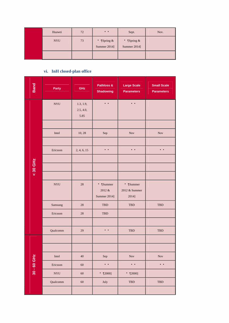
a. Overview of measurement campaigns
The basis for this white paper is the open literature in combination with recent and ongoing
propagation channel measurements performed by the cosignatories of this white paper, some of
which are as yet unpublished. The following tables give an overview of these recent measurement
activities in different frequency bands and scenarios.
i. UMi street canyon O2O
Ban
d
Party GHzPathloss &
Shadowing
Large Scale
Parameters
Small Scale
Parameters
NYU 1.8 ● ● ●
CMCC 6 ● ● Aug.
DCM 8 ●
CMCC 10 TBD TBD
Intel 10 July. Sep. Sep.
Nokia/Aalborg 2, 10, 18 ●
CMCC 14 Sep. Sep.
Aalto 15 Sep. Sep. Sep.
Huawei 15
Ericsson 15 ● ● ●
DCM 20, 26 ● Sep. (20) Sep. (20)
Huawei 28 ● Nov. Nov.
Intel 28 Sep. Nov. Nov.
NYU 28 ● [Summer
2012]
● [Summer
2012]
● [Summer 2012]
NYU 28 Sep. Sep. Sep.
Samsung 28 ● ● ●
Ericsson 28
Nokia/Aalborg 28 ● ●
< 30
GH
z
CMCC 28 Sep. Sep.

Aalto 28 ● ● ●
Qualcomm 29 Oct. TBD TBD
Ban
d
Party GHzPathloss &
Shadowing
Large Scale
Parameters
Small Scale
Parameters
Huawei 30-40
DCM 37 ●
NYU 38
Intel 40, 60 July (60)
Sep. (40)
Sep (60)
Nov. (40)
Sep. (60)
Nov. (40)
Ericsson 60
Huawei 60 Nov. Nov. Nov.
Qualcomm 60 Oct. TBD TBD
30- 6
0 G
Hz
Aalto 63 Sep. Sep. Sep.
Huawei 73 ● Nov. Nov.
NYU 73 ● [Summer
2013 ]
● [Summer
2013 ]
● [Summer
2013 ]
Intel 75, 82 Sep. Nov. Nov.
>60
GH
z
ii. UMi open square O2O
Ban
d
Party GHzPathloss &
Shadowing
Large Scale
Parameters
Small Scale
Parameters
Nokia / AAU 10 ● Madrid-grid
CMCC 14 Sep. Sep.
< 30
GH
z
Nokia / AAU 2, 10,18 ●

Nokia/AAU 28 ●
Samsung 28 TBD
(July or Sep)
TBD (Sep) TBD (Sep)
Qualcomm 29 ● TBD TBD
Qualcomm 60 Sept TBD TBD
Univ. of Bristol 60 TBD (Spring
2016)
TBD (Spring
2016)
TBD (Spring 2016)
30-6
0 G
Hz
Aalto 63 ● ● ●
NYU 73 ● [Spring
2014]
● [Spring 2014]
> 60
GH
z
iii. UMi O2I
Ban
d
Party GHzPathloss &
Shadowing
Large Scale
Parameters
Small Scale
Parameters
NYU 1.9, 5.85 ●
DCM 8, 26 July
Nokia/Aalborg 10 ●
Ericsson 6, 15, 28 ● ● ●
Nokia/Aalborg 20 ●
Nokia/Aalborg 28 Sep.
Samsung 28 TBD (July)
NYU 28 ● [Summer
2012]
● [Summer
2012]
< 30
GH
z
Ericsson 28

DCM 37 July
Ericsson 60 ● ● ●
30-6
0 G
Hz
> 60
GH
z
iv. UMa O2O
Ban
d
Party GHzPathloss &
Shadowing
Large Scale
Parameters
Small Scale
Parameters
CMCC 6 Sep. Sep.
Nokia/Aalborg 2, 10, 18,
28
●
CMCC 14 TBD TBD
< 30
GH
z
NYU 38 ● [Summer
1998 &
Summer 2011]
● [Summer
1998 & Summer
2011]
30-6
0 G
Hz
> 60
GH
z
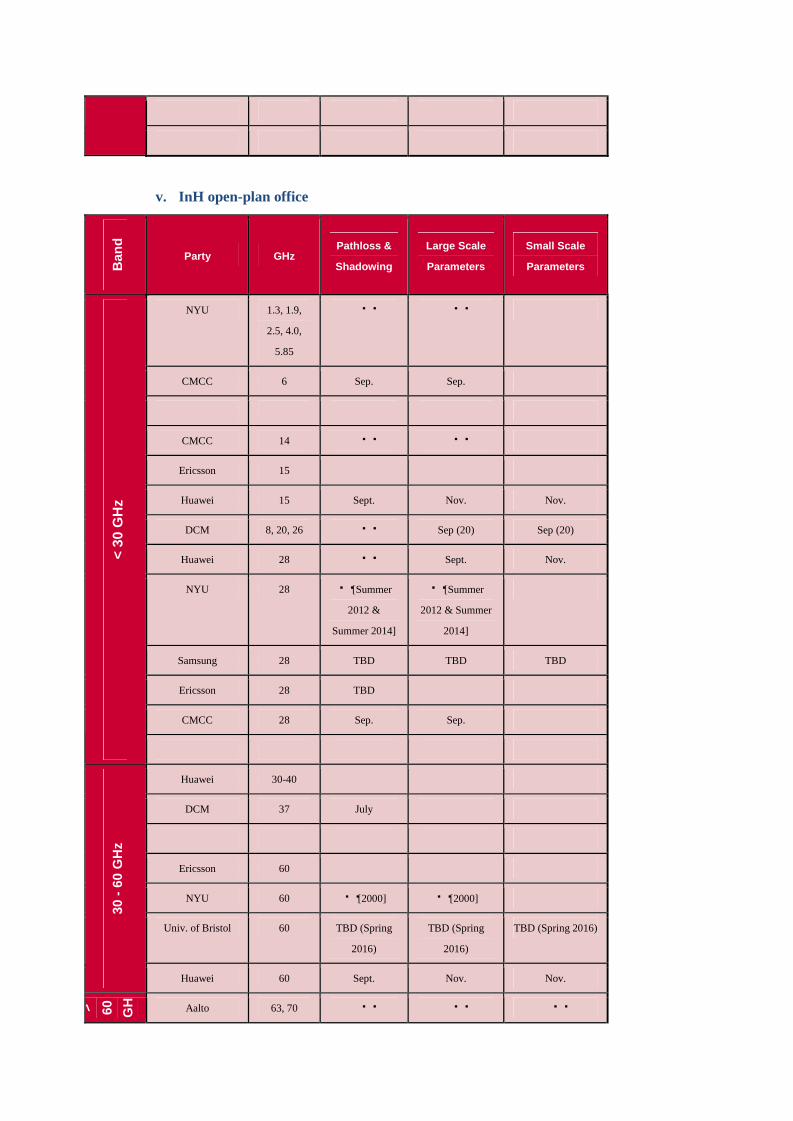
v. InH open-plan office
Ban
d
Party GHzPathloss &
Shadowing
Large Scale
Parameters
Small Scale
Parameters
NYU 1.3, 1.9,
2.5, 4.0,
5.85
● ●
CMCC 6 Sep. Sep.
CMCC 14 ● ●
Ericsson 15
Huawei 15 Sept. Nov. Nov.
DCM 8, 20, 26 ● Sep (20) Sep (20)
Huawei 28 ● Sept. Nov.
NYU 28 ● [Summer
2012 &
Summer 2014]
● [Summer
2012 & Summer
2014]
Samsung 28 TBD TBD TBD
Ericsson 28 TBD
CMCC 28 Sep. Sep.
< 30
GH
z
Huawei 30-40
DCM 37 July
Ericsson 60
NYU 60 ● [2000] ● [2000]
Univ. of Bristol 60 TBD (Spring
2016)
TBD (Spring
2016)
TBD (Spring 2016)
30-6
0 G
Hz
Huawei 60 Sept. Nov. Nov.
> 60 GH z Aalto 63, 70 ● ● ●
Huawei 72 ● Sept. Nov.
NYU 73 ● [Spring &
Summer 2014]
● [Spring &
Summer 2014]
vi. InH closed-plan office
Ban
d
Party GHzPathloss &
Shadowing
Large Scale
Parameters
Small Scale
Parameters
NYU 1.3, 1.9,
2.5, 4.0,
5.85
● ●
Intel 10, 28 Sep Nov Nov
Ericsson 2, 4, 6, 15 ● ● ●
NYU 28 ● [Summer
2012 &
Summer 2014]
● [Summer
2012 & Summer
2014]
Samsung 28 TBD TBD TBD
Ericsson 28 TBD
< 30
GH
z
Qualcomm 29 ● TBD TBD
Intel 40 Sep Nov Nov
Ericsson 60 ● ● ●
NYU 60 ● [2000] ● [2000]
Qualcomm 60 July TBD TBD
30-6
0 G
Hz

Aalto 63, 70 ● ● ●
NYU 73 ● [Spring &
Summer 2014]
● [Spring &
Summer 2014]> 60
GH
z
Intel 75, 82 Sep. Nov Nov
vii. InH shopping mall
Ban
d
Party GHzPathloss &
Shadowing
Large Scale
Parameters
Small Scale
Parameters
CMCC 6 TBD TBD
Nokia/Aalborg 2, 10, 18 ●
Intel 10, 28 Sep. Nov Nov
CMCC 14 Jul. Jul.
Aalto 15 ● ● ●
Aalto 28 ● ● ●
Samsung 28 ● ● ●
Nokia/Aalborg 28 Sep.
< 30
GH
z
Qualcomm 29 June TBD
Intel 40 Sep. Nov Nov
Qualcomm 60 June TBD
Univ. of Bristol 60 TBD (Spring
2016)
TBD (Spring
2016)
TBD (Spring 2016)
30-6
0 G
Hz
Aalto 63, 70 ● ● ●
Intel 75, 82 Sep. Nov Nov
> 60
GH
z
b. Overview of ray-tracing campaigns
i. UMi street canyon O2O

Ban
dParty GHz
Pathloss &
Shadowing
Large Scale
Parameters
Small Scale
ParametersLocation Details
Aalto 15 Nov. Nov. Nov. Greater Helsinki area
Aalto 28 Nov. Nov. Nov. Greater Helsinki area
Samsung 28 ● ● ● Daejeon, Korea
/ Same location for
measurement
campaign
Samsung 28 ● ● ● Ottawa
Samsung 28 ● ● ● NYU Campus
/ Same location for
NYU measurement
campaign
USC 28 ● ● ●
< 30
GH
z
Nokia 5.6,10.25,
28.5
● ● ● Madrid-grid
Nokia 39.3 ● ● ● Madrid-grid
30-6
0 G
Hz
Aalto 63 Nov. Nov. Nov. Greater Helsinki area
Nokia 73 ● ● ● NYU Campus plus
Madrid-grid
> 60
GH
z
ii. UMi open square O2O
Ban
d
Party GHzPathloss &
Shadowing
Large Scale
Parameters
Small Scale
Parameters
Location
Details

Nokia 5.6,10.25,
28.5
● ● ● Madrid-grid
Univ. of Bristol 28 TBD (Spring
2016)
TBD (Spring
2016)
TBD (Spring 2016) Bristol / London
< 30
GH
z
Nokia 39.3 ● ● ● Madrid-grid
Univ. of Bristol 40 / 60 TBD (Spring
2016)
TBD (Spring
2016)
TBD (Spring 2016) Bristol / London
30-6
0 G
Hz
Aalto 63 ● ● ● Helsinki city
center
Nokia 73.5 ● ● ● Madrid-grid
> 60
GH
z
iii. UMa O2O
Ban
d
Party GHzPathloss &
Shadowing
Large Scale
Parameters
Small Scale
Parameters
Location
Details
Nokia 5.6,10.25,
28.5
● ● ● Madrid-grid
Nokia/Aalborg 10, 18, 28 Sep. Sep. Oct. Aalborg (same
location as
measurement
campaigns)
Samsung 28 ● ● ● Ottawa
Samsung 28 ● ● ● NYU Campus
< 30
GH
z
Univ. of Bristol 28 TBD (Spring
2016)
TBD (Spring
2016)
TBD (Spring 2016) Bristol / London

Univ. of Bristol 40 / 60 TBD (Spring
2016)
TBD (Spring
2016)
TBD (Spring 2016) Bristol / London
Nokia/Aalborg 39.3 Sep. Sep. Oct. Aalborg (same
location as
measurement
campaigns)
Nokia 39.3 ● ● ● Madrid-grid
30-6
0 G
Hz
Nokia/Aalborg 73.5 Sep. Sep. Oct. Aalborg (same
location as
measurement
campaigns)
Nokia 73.5 ● ● ● Madrid-grid
> 60
GH
z
iv. InH open-plan office
Ban
d
Party GHzPathloss &
Shadowing
Large Scale
Parameters
Small Scale
ParametersLocation Details
Samsung 28 TBD TBD TBD (Sep) Open-Office
< 30
GH
z30
-60
GH
z

Nokia 73 ● ● ● Open-office at
NYU campus>
60 G
Hz
v. InH closed-plan office
Ban
d
Party GHzPathloss &
Shadowing
Large Scale
Parameters
Small Scale
ParametersLocation Details
< 30
GH
z30
-60
GH
z
Aalto 63, 70 ● ● ● Large office,
meeting room,
cafeteria
> 60
GH
z
vi. InH shopping mall
Ban
d
Party GHzPathloss &
Shadowing
Large Scale
Parameters
Small Scale
ParametersLocation Details

Samsung 28 TBD TBD TBD (Sep) Shopping-mall like
environment
/ Same location for
measurement
campaign
< 30
GH
z30
-60
GH
z
Aalto 63, 70 ● ● ● A shopping mall in
Helsinki area
> 60
GH
z
c. Fast Fading Models
UMi
Table 7. Preliminary UMi channel model parameters.
28 GHz1 73 GHz2
LoS NLoS LoS (28-73 Combined) NLoS
DS -8.70 -7.39 -7.71 -7.52Delay spread ()
log10
(seconds) DS 0.54 0.31 0.34 0.50
ASA -0.49 1.42 1.69 1.45AoA spread (
ASA)
log10
(degrees) ASA 0.93 0.29 0.27 0.32
ASD -0.40 0.82 1.28 1.32AoD spread (
ASD)
log10
(degrees) ASD 1.07 0.38 0.50 0.38
ZSA -1.40 0.69 0.60 0.53ZoA spread (
ZSA)
(degrees) ZSA 1.09 0.40 0.09 0.15

ZSD -1.25 -0.21 N/A 0.46ZoD spread (
ZSD)
(degrees) ZSD 0.04 0.30 N/A 0.18
Shadow fading (dB) 0.63 22.09 3.6 (28 G) - 5.2 (73 G) 7.60
Delay distribution Exponential distribution
AoD and AoA distribution Laplacian distribution Uniform [0, 360]
ZoD and ZoA distribution Laplacian distribution Gaussian distribution
Delay scaling parameter 4.42 4.82 3.90 3.10
XPR TBD TBD TBD TBD
XPR (dB)
XPR TBD TBD TBD TBD
Table 8. Preliminary UMi cluster parameters
28 GHz1 73 GHz2
LoS NLoSLoS
(28-73 Combined)NLoS
Clustering Algorithm K-Means algorithm K-Means algorithm
Ave. number of clusters 6 6 5.0 4.6
Ave. number of rays per cluster 10 10 12.4 13.2
Cluster DS (nsec) TBD TBD TBD TBD
Cluster ASA (degrees) 3.3 6.7 6.7 5.2
Cluster ASD (degrees) 2.7 5.7 1.5 2.1
Cluster ZSA (degrees) 3.9 4.9 1.8 1.5
Cluster ZSD (degrees) 1.2 1.6 N/A 0.8
Per-cluster shadow fading (dB) 5 5 13.6 17.4
Table 9. Preliminary UMi correlations for large-scale parameters
28 GHz1 73 GHz2
LoS NLoS LoS(28-73 Combined) NLoS
ASD vs. DS -0.25 0.37 0.32 0.054
ASA vs. DS 0.35 0.43 0.49 0.282
ASA vs. SF -0.01 0.03 0.54 0.042
ASD vs. SF -0.24 0.16 -0.04 0.009
DS vs. SF 0.22 0.30 0.35 -0.177
ASD vs. ASA -0.67 0.09 0.72 -0.256
ZSD vs. SF 0.23 0.13 N/A -0.430
ZSA vs. SF 0.16 0.10 0.16 -0.389
ZSD vs. DS 0.27 0.50 N/A 0.950
ZSA vs. DS 0.14 0.19 0.44 0.108
ZSD vs. ASD -0.32 0.36 N/A 0.49

ZSA vs. ASD -0.39 0.10 0.95 -0.263
ZSD vs. ASA 0.33 0.20 N/A 0.950
ZSA vs. ASA 0.37 0.02 0.72 0.232
ZSD vs. ZSA 0.92 0.52 N/A -0.960
3. From Samsung based on ray-tracing
4. From NYU based on measurement [Samimi EUCAP2016]
UMa
Table 10. Preliminary UMa NLOS channel model parameters.
5.6 GHz 10 GHz 18 GHz 28 GHz 39.3 GHz 73.5 GHz
DS -6.75 -6.80 -6.85 -6.88 -6.89 -6.91Delay spread ()
log10
(seconds) DS 0.68 0.88 0.78 0.73 0.73 0.69
ASA 1.34 1.14 1.14 1.15 1.14 1.09AoA spread
(ASA
)
log10
(degrees)
ASA 0.81 1.14 1.01 0.94 0.91 0.87
ASD 0.87 0.67 0.74 0.75 0.78 0.82AoD spread
(ASD
)
log10
(degrees)
ASD 0.81 1.35 1.05 1.16 1.06 0.93
ZSA 0.48 0.31 0.26 0.26 0.24 0.20ZoA spread
(ZSA
)
log10(degrees)
ZSA 0.75 0.92 0.85 0.81 0.81 0.79
ZSD -0.26 -0.24 -0.22 -0.22 -0.20 -0.16ZoD spread
(ZSD
)
log10(degrees)
ZSD 0.70 0.74 0.78 0.81 0.82 0.83
Shadow fading (dB) 9.82 10.22 10.28 10.12 10.14 9.97
Delay distribution Exponential Exponential Exponential Exponential Exponential Exponential
AoD and AoA distribution Laplacian Laplacian Laplacian Laplacian Laplacian Laplacian
ZoD and ZoA distribution Laplacian Laplacian Laplacian Laplacian Laplacian Laplacian
Delay scaling parameter TBD TBD TBD TBD TBD TBD
XPR 13.87 12.94 10.97 10.76 9.38 7.89
XPR (dB)
XPR 6.12 6.36 6.80 6.57 6.60 6.38
Table 11. Preliminary UMa NLOS cluster parameters
Note that the ray tracer for the Uma scenario was run with only a total of 20 rays, so some clustering
parameters, particularly the number of rays per cluster, may be low.

5.6 GHz 10 GHz 18 GHz 28 GHz 39.3 GHz 73.5 GHz
K-Means
Ave. number of clusters 3.78 4.21 4.09 4.10 4.05 4.05
Ave. number of rays per
cluster5.89 4.66 4.97 5.05 5.10 5.19
Cluster DS (nsec) 77.97 56.79 57.61 50.41 49.63 50.72
Cluster ASA (degrees) 9.96 7.85 7.67 7.31 7.39 7.06
Cluster ASD (degrees) 4.54 4.46 4.53 4.32 4.27 4.28
Cluster ZSA (degrees) 3.70 2.71 2.38 2.34 2.39 2.29
Cluster ZSD (degrees) 0.69 0.85 0.84 0.81 0.83 0.85
Per-cluster shadow fading
(dB)6.12 5.86 5.82 5.67 5.46 4.87
Table 12. Preliminary UMa NLOS correlations for large-scale parameters
5.6 GHz 10 GHz 18 GHz 28 GHz 39.3 GHz 73.5 GHz
ASD vs. DS 0.67 0.65 0.59 0.56 0.54 0.53
ASA vs. DS 0.06 0.09 0.06 0.06 0.05 0.04
ASA vs. SF 0.04 0.04 0.05 0.00 0.01 -0.04
ASD vs. SF -0.18 -0.17 -0.22 -0.23 -0.25 -0.28
DS vs. SF -0.05 -0.21 -0.15 -0.18 -0.20 -0.20
ASD vs. ASA -0.02 0.01 0.07 0.07 0.05 0.07
ZSD vs. SF -0.32 -0.39 -0.43 -0.43 -0.44 -0.47
ZSA vs. SF 0.21 0.17 0.15 0.08 0.07 -0.01
ZSD vs. DS 0.34 0.41 0.36 0.35 0.35 0.33
ZSA vs. DS -0.26 -0.20 -0.17 -0.15 -0.17 -0.14
ZSD vs. ASD 0.73 0.72 0.73 0.73 0.74 0.75
ZSA vs. ASD -0.33 -0.26 -0.19 -0.18 -0.15 -0.06
ZSD vs. ASA 0.08 0.16 0.25 0.27 0.27 0.30
ZSA vs. ASA 0.54 0.54 0.60 0.62 0.61 0.62
ZSD vs. ZSA -0.08 0.01 0.06 0.09 0.14 0.25
InH
Table 13. Preliminary InH large-scale channel characteristics
20 GHz1 28GHz2 60 GHz2 73GHz3 73GHz4
Indoor office Shopping mall Shopping mall Indoor office Indoor officeScenario
LOS LOS NLOS LOS NLOS Hybrid Hybrid
DS -7.33 -7.52 -7.59 -7.62 -7.45 -8.1 N/ADelay spread ()
log10
(seconds) DS 0.1 0.17 0.33 0.20 0.11 0.4 N/A

Delay distribution N/A Exponential Exponential N/A
ASA N/A 1.54 1.57 1.50 1.60 1.6 N/AAoA spread (
ASA)
log10
(degrees) ASA N/A 0.16 0.18 0.16 0.15 0.37 N/A
ASD 1.8 1.44 1.68 1.43 1.72 1.5 N/AAoD spread (
ASD)
log10
(degrees) ASD 0.09 0.16 0.19 0.10 0.08 0.26 N/A
ZSA N/A 0.87 0.68 0.86 0.67 -0.025d+1.18 N/AZoA spread (
ZSA)
(degrees) ZSA N/A 0.45 0.31 0.40 0.23 0.30 N/A
ZSD 0 0.75 0.95 0.74 0.88 -0.040d+1.45 N/AZoD spread (
ZSD)
(degrees) ZSD 0.48 0.34 0.22 0.30 0.20 0.33 N/A
AoD and AoA distribution N/A Wrapped Gaussian Uniform N/A
ZoD and ZoA distribution N/A Laplacian Laplacian N/A
XPR N/A 16.12 14.48 16.85 16.06 15 11
XPR (dB)
XPR N/A 6.22 6.26 6.62 5.34 2 6.5
K N/A -0.18 n/a -1.07 n/a 8 N/ALOS Ricean K factor
(dB) * K N/A 2.85 n/a 3.58 n/a 3 N/A
1. From DOCOMO based on measurement
2. From Aalto University based on measurement
3. From Nokia/NYU based on ray-tracing
4. From Huawei based on measurement
d. Processing Methodologies
i. Physical effects on propagation
As a consequence of shorter wavelengths as the carrier frequency increases, the radio propagation
must be modelled with an understanding and consideration of a number of physical effects that occur
in the real environment. A deployment scenario, perhaps involving up to a hundred meters of
propagation transmission distance with short wavelengths, will encounter multiple different physical
transmission effects. It is helpful if these physical effects are included in the overall transmission
model to accurately reflect the behavior of the radio propagation environmental conditions.
An illustration of some of the physical effects of propagation is shown in Figure 17. This illustration
may be helpful in understanding the multiple regions of physical processes that may be in the
environment and affect the radio propagation.
Zone1 (close range free space)
Propagation is dominated by the direct path with few reflections.
Zone 2 (LOS/scattered/waveguide)
Propagation is dominated by the direct path and significant close reflections.
Zone 3 (NLOS occultation scattered)
Propagation is mainly by the reflections with some direct path energy but these are attenuated
by distance.
Zone 4 (distant NLOS)

Propagation is dominated by a small number of paths that are either not occulted or are a result
of a good reflection.
Zone 5 (too distant)
The illustration also shows a fifth zone in which the signals have become too weak to be useful
either through numerous multiple reflections, distance, corners or occultation. In this zone
communications is generally impractical.
Figure 17. Illustration of multiple physical transmission effects
In each region there is always the possibility of physical blockage or occultation. Because of the small
wavelengths, many typical objects in the environment (e.g. people, furniture, machinery, office
equipment, etc.) are of a size that they completely block the direct signal, leaving the receiver with
little except whatever reflections that may be available. This is shown in the illustration as typically
in Zone 3 or 4 but it may occur anywhere. Also in some instances, there may be penetration loss for
signals into interior rooms or through walls. The zone size depends on the wavelength, the
dimensions and details of the environment, and the antenna beam widths. Not all zones may exist in
every deployment environment or signal path. Typically, the signal propagation may experience
multiple physical effects on its journey and so the “zones” may overlap in space.
ii. The effects of the antenna pattern
In understanding the measurements of the new 5G channels and the associated channel model
parameters, it is helpful to know the characteristics of the antennas used to make the measurements.
Some measurement antennas are directive (e.g. horn or array antennas) and consequently may not
illuminate reflecting surfaces of the environment during measurements and thus may appear to
simplify the environment when compared with measurements made with other non-directional
antennas (e.g. omni-directional antennas). In some cases, the test antennas may have significant
sidelobes in their radiation pattern and these may make the environment seem more reflective than is
physically the case.
Traditionally, measurements in the frequency bands below 6 GHz have used omni-directional
antennas. In these bands the transmit antenna “floods” the environment with power in all directions(i.e. sector coverage) and the receive antenna accepts power from all directions at its location. In

environments in which there are many reflections the apparent “path loss” may be reduced due to theadditional power received from the many reflections. Typically in low frequency bands, the same
antenna format (i.e. sector at base station and omni-directional at user equipment) is also used for the
operational equipment and so the total-power/omni-directional path loss measurement is appropriate
for the operating environment. Propagation studies and operation for these bands has thus been
successful because the measurements, modelling and operation are all based on similar antenna
characteristics.
In the bands above 6 GHz however, directional antennas (e.g. “horns”) are often used formeasurements to help improve the range of the measurements. Directional antenna configurations
are also expected to be used for operational equipment including mobile devices and access points as
the antenna “gain” they provide may be necessary in the operational system to achieve the needed link
budget. However, if the antenna configuration used for the path loss measurements is not the same
as used for the operating equipment, then the associated model may not be accurate for modelling link
budgets for equipment having different antenna configurations. Equipment with a narrow beam
antenna will typically see less received power than would be expected based on a path loss model
derived from measurements using omni-directional antennas.
a. Decoupling the antenna pattern
Many of the future systems will be operated using highly directional antennas for at least a portion of
their usage. To accurately model these conditions it is necessary to decouple the channel model
from the measurement antenna patterns. This is often referred to as “antenna decoupling”. Themeasurements are in reality the convolution of the measurement antenna patterns and the channel
environment and recovering the channel environment from the measurements involves a
“deconvolution” of the measuring antenna patterns from the measurements. The general process for
decoupling of the antenna pattern to reconstruct the true signal angular distribution can be
summarized in the following steps.
1. Estimate the path of propagation (angular domain/delay domain/both).
2. Remove the antenna pattern (different algorithms).
3. Reconstruct the estimated measured data with antenna pattern.
4. Evaluate the effect of reconstruction and antenna decoupling.
For a typical measurement antenna with a main beam and small side-lobes, the measured angular
spectrum will appear as the actual channel “blurred” by the measurement antenna sampling pattern.To recover the true angular distribution of the actual channel it is necessary to undo the convolution
between the measuring antenna and the channel. This is not an easy to do as practical signals and
beam patterns include zeros or low amplitude regions that may prevent a simple analytical inversion
from recovering the real channel. However, with sufficiently well behaved signals (i.e. with
well-defined angular clusters and a good ratio between beam strength and its side-lobes) often a good
approximations can be made.
Similar measurement decoupling problems are experienced in a number of other sciences and there
are several algorithms for deriving the hypothetical true angular distribution from the data. Some of
these processes are iterative, in which an initial estimate is gradually corrected based on its
comparison to the measured data. A popular practical technique in the RADAR community is the
“MUSIC” algorithm [Schmidt] while the Synthetic Aperture Imaging and radio astronomy

communities use the “CLEAN” algorithm [Clarke]. The SAGE algorithm has also been applied inthis context [Fessler].
iii. Variant angles modeling for beam-tracking
A new feature for 5G communications, particularly in higher frequency bands, is that large antenna
arrays or high-gain, directional antennas may be utilized in base-stations (BS) and potentially in user
equipment (UE) in order to compensate for the larger propagation loss of signals above 6 GHz. The
resulting beams will have small beam-widths making the transmission link sensitive to changes in
angles of departure and arrival of the propagation paths between BS and UE. Modeling of the
variability of angles of multipath components will enable studies of the robustness and performance
evaluation of techniques such as beam-tracking. While this white paper does not provide any
recommendation on the modelling methodology at this stage, it is worth mentioning some of the
proposed approaches.
Variant angle model has been studied in WINNER project in [WINNER] and recently was developed
to 3GPP 3D channel model with linear approximation method in [Wang2015]. Both of them are in the
framework of spatial channel model (SCM) with low computational complexity. Other solutions for
variant angles include the map-based channel model in METIS [METIS 2015] and the COST2100
MIMO model [Liu2012]
iv. Clustering
Different clustering algorithms were considered in support of the channel modelling activities herein
described. These algorithms include the Agglomerative algorithm, the k-means algorithm and the time
cluster and spatial lobe clustering algorithm.
The agglomerative algorithm is a bottom-up hierarchical clustering algorithm where multipath
components (MPCs) are iteratively merged together. It starts with each MPC belonging to a different
cluster and, at each step, the most similar clusters are combined. The process repeats until either a
stop criterion is met or only one single cluster remains.
The K-means algorithm [Czink VTCF06] groups the multipath components (MPCs) into clusters
such that the MPCs within each cluster have similar delay, elevation and azimuth angles. The
algorithm identifies each cluster by its centroid position in the parameter space. Each MPC is assigned
to the cluster centroid with smallest distance. The algorithm iteratively optimizes the positions of the
centroids in order to minimize the total distance from each MPC to its centroid.
In the time cluster and spatial lobe clustering algorithm approach [Samimi GCW2015][SamimiICC2015] [Samimi EUCAP2016], the time and space dimensions are considered independently, byseparately performing data clustering in the temporal and spatial domains, yielding statistics for time
clusters and spatial lobes in omnidirectional millimeter wave channels. Time clusters are composed of
multipath components traveling close in time delay, and that arrive from potentially different angular
directions in a short propagation time window as seen from field measurements. Spatial lobes
represent main directions of arrival (or departure) where energy arrives over the entire time span of
the multipath time delay profile. In this modeling framework, a channel impulse response “initialcondition” for a particular location or point is generated by separately generating time cluster
parameters and spatial lobe parameters independently, and then randomly assigning the different

multipath components to different spatial lobes as has been found to occur in millimeter wave
channels.
This paper reflects the outcome from an ad-hoc industry working group that included the following
participants.
Company Contact name Email Address
8 Aalto University Katsuyuki Haneda [email protected]
BUPT Lei Tian [email protected]
CMCC Yi Zheng [email protected],
Ericsson Henrik Asplund [email protected]
Huawei Li Jian, Yi Wang, David Steer [email protected],
INTEL Clara Li, Tommaso Balercia [email protected],
KT Corporation Sunguk Lee, YoungSuk Kim [email protected],
Nokia Amitava Ghosh, Tim Thomas amitava.ghosh, @nokia.com,
NTT DOCOMO Takehiro Nakamura, Yuichi
Kakishima, Tetsuro Imai,
Haralabos Papadopoulas
hpapadopoulos@
docomoinnovations.com
NYU Theodore (Ted) S. Rappaport,
George R. MacCartney,
Mathew K. Samimi, Shu Sun
Qualcomm Ozge Koymen [email protected]
Samsung Sooyoung Hur, Jeongho Park,
Charlie Zhang
University of Bristol Evangelos Mellios [email protected]
University of Southern
California
Andreas F.Molisch [email protected]

References
[3GPP TR25.996] 3GPP TR 25.996 (V.12.0.0), “Spatial channel model for Multiple Input MultipleOutput (MIMO) simulations,” Sep. 2014.
[3GPP TR36.814] 3GPP TR 36.814 (V9.0.0), “Further advancements for E-UTRA physical layer
aspects ,” Mar. 2010.
[3GPP TR36.873] 3GPP, TR 36.873 (V12.2.0), “Study on 3D channel model for LTE,” July 2015
[Andersen 1995] J. Andersen, T. Rappaport, and S. Yoshida, “Propagation measurements and modelsfor wireless communications channels,” IEEE Communications Magazine, vol. 33, no. 1, pp. 42–49,
Jan 1995.
[And2002] C. Anderson, et. al., “In-Building Wideband Multipath Characteristics at 2.5 & 60 GHz,”2002 IEEE Vehicular Technology Conference, Fall 2002.
[Baum2015] D. S. Baum, J. Hansen, and J. Salo, “An interim channel model for beyond-3G systems:
extending the 3GPP spatial channel model (SCM),” in Proc. IEEE VTC-spring, vol. 5, 2005,
pp.3132-3136.
[Clark Sept. 1980] An efficient implementation of the algorithm 'CLEAN'; Clark, B. G.; Astronomy
and Astrophysics, vol. 89, no. 3, pp377-378; Sept 1980.
[COST] http://www.cost2100.org/
[Czink VTCF06] N. Czink, et al., “A framework for automatic clustering of parametric MIMOchannel data including path powers,” in IEEE VTC-Fall 2006, September 2006.
[ETSI 2015] ETSI, “New ETSI Group on Millimetre Wave Transmission starts work,”http://www.etsi.org/news-events/news/866-2015-01-press-new-etsi-group-on-millimetre-wave-transm
ission-starts-work
[Fessler VTC Fall 2014] Space-Alternating Generalized Expectation-Maximization Algorithm;
Fessler, J.A.; IEEE Transactions on Signal Processing, vol. 42, no. 10, pp2664-2677; Oct 1994.
[Gustafson 2014] C. Gustafson, et. al. , “On mm-Wave Multipath Clustering and Channel
Modeling,”,IEEE Transactions on Antennas and Propagation, vol. 62, no. 3, pp. 1445-1455, March
2014.
[Hata 1980] M. Hata, “Empirical formulas for propagation loss in land mobile radio service,” IEEETrans. Veh. Technol., vol. 29, no. 3, pp. 317–325, Aug.1980
[Hur EuCAP2015-1] S. Hur, et. al.,“Wideband Spatial Channel Model in an Urban CellularEnvironments At 28 GHz,” in Proc. EuCAP2015, April 2015.

[Hur EuCAP2015-2] S. Hur, et. Al., “28 GHz Channel Modeling Using 3D Ray-Tracing in Urban
Environments”, in Proc. EuCAP2015, April 2015.
[ITU M.2135-1] ITU-R Rep M.2135-1, ”Guidelines for evaluation of radio interface technologies for
IMT-Advanced.”
[Karttunen EuCAP2015] A. Karttunen, K. Haneda, J. Jarvelainen and J. Putkonen, “PolarisationCharacteristics of Propagation Paths in Indoor 70 GHz Channels,” in Proc. 9th European Conf. Ant.
Prop. (EuCAP 2015), Lisbon, Portugal, Apr. 2015.
[Larsson EuCAP 2014] C. Larsson, F. Harrysson, B-E. Olssson and J-E. Berg, "An outdoor-to-indoor
propagation scenario at 28 GHz", in Proc. of European Conference on Antennas and Propagation
(EuCAP) 2014, pp. 3301-3304.
[Liu2012] L. Liu, C. Oestges, J. Poutanen, K. Haneda, P. Vainikainen, F. Quitin, F. Tufvesson, P. D.
Doncker, “The COST 2100 MIMO channel model,”, IEEE Wireless Communications Magazine, Dec.,2012, pp. 92-99.
[MacCartney GC2013] G. MacCartney, J. Zhang, S. Nie, and T. Rappaport, “Path loss models for 5gmillimeter wave propagation channels in urban microcells,” in 2013 IEEE Global Communications
Conference (GLOBECOM), Dec. 2013, pp. 3948–3953.
[MacCartney 2015], G. MacCartney, et. al, “Indoor Office Wideband Millimeter-Wave Propagation
Measurements and Channel Models at 28 GHz and 73 GHz for Ultra-Dense 5G Wireless Networks,”IEEE Access, October 2015.
[METIS 2013] “Simulation Guidelines,” Deliverable D6.1, METIS document numberICT-317669-METIS/D6.1, October 31, 2013.
[METIS 2015] METIS2020, Deliverable D1.4 v3, “METIS Channel Model,” July 2015.https://www.metis2020.com/wp-content/uploads/METIS_D1.4_v3.pdf
[MiWEBA 2014] MiWEBA, Deliverable D5.1 “Channel modeling and characterization,” June,2014, http://www.miweba.eu/wp-content/uploads/2014/07/MiWEBA_D5.1_v1.011.pdf.
[mmMagic] https://5g-ppp.eu/mmmagic/
[Nie13] S. Nie, G. R. MacCartney, Jr., S. Sun, T. S. Rappaport, “72 GHz Millimeter Wave IndoorMeasurements for Wireless and Backhaul Communications,” in 2013 IEEE 24th Annual International
Symposium on Personal, Indoor and Mobile Radio Communications, (PIMRC), Sept. 2013, pp.
2429.
[NIST] http://www.nist.gov/ctl/wireless-networks/5gmillimeterwavechannelmodel.cfm
[Nguyen16] H. C. Nguyen, et al., “An Empirical Study of Urban Macro Propagation at 10, 18, and 28GHz,” submitted to VTC-2016/Spring.
[Piersanti ICC2012] S. Piersanti, L. Annoni, and D. Cassioli, “Millimeter waves channelmeasurements and path loss models,” in 2012 IEEE International Conference on Communications
(ICC), June 2012, pp. 4552–4556.
[Rappaport 2013] T. S. Rappaport et al., "Millimeter Wave Mobile Communications for 5G Cellular:
It Will Work!," in IEEE Access, vol.1, pp. 335-349, 2013.

[Rappaport 2015], T. S. Rappaport, et. al.,” Wideband Millimeter-Wave Propagation Measurements
and Channel Models for Future Wireless Communication System Design,” IEEE Trans.Communications,” Vol. 63, No. 9, , pp. 3029-3056, Sept. 2015.
[Rappaport Book2015] T. S. Rappaport, R. W. Heath, Jr., R. C. Daniels, and J. N. Murdock,
Millimeter Wave Wireless Communications. Pearson/Prentice Hall 2015.
[Rodriguez VTC Fall 2014] I. Rodriguez, H. C. Nguyen, N. T. K. Jorgensen, T. B. Sorensen and P.
Mogensen, "Radio Propagation into Modern Buildings: Attenuation Measurements in the Range from
800 MHz to 18 GHz", in Proc. of IEEE Vehicular Technology Conference (VTC fall), 2014, pp. 1-5.
[Samimi 2015] M. K. Samimi, T. S. Rappaport, and G. R. MacCartney, Jr., “Probabilisticomnidirectional path loss models for millimeter-wave outdoor communications,” in IEEE Wireless
Communications Letters, vol. 4, no. 4, pp. 357-360, Aug. 2015.
[Samimi GCW2015] M. K. Samimi, T. S. Rappaport, “3-D Statistical Channel Model for
Millimeter-Wave Outdoor Communications,” in 2015 IEEE Global Communications Conference,Exhibition & Industry Forum (GLOBECOM) Workshop, Dec. 6-10, 2015.
[Samimi EUCAP2016] M. K. Samimi, T. S. Rappaport, “Local Multipath Model Parameters forGenerating 5G Millimeter-Wave 3GPP-like Channel Impulse Response,” submitted to the 10thEuropean Conference on Antennas and Propagation (EuCAP’2016), April 2016
[Schmidt Mar 1986] Multiple emitter location and signal parameter estimation; Schmidt, R.O. ; IEEE
Transactions on Antennas and Propagation, vol. 34, Issue: 3; pp276-280; Mar1986.
[Semaan Globecom 2014] E. Semaan, F. Harrysson, A. Furuskär and H. Asplund, "Outdoor-to-indoor
coverage in high frequency bands", Globecom Workshops 2014, pp. 393-398.
[Sun GCW2015], S. Sun, et. al., “Path Loss, Shadow Fading, and Line-Of-Sight Probability Models
for 5G Urban Macro-Cellular Scenarios,” 2015 IEEE Globecom Workshop, San Diego, Dec. 2015.
[Sun VTCS2016] S. Sun, et al., “Path Loss Models for 5G Urban Micro- and Macro-Cellular
Scenarios,” submitted to IEEE VTC-Spring 2016, May 2016.
[Tenerelli1998] P. A. Tenerelli and C. W. Bostian, “Measurement of 28 GHz diffraction loss bybuilding corners”, in Proc. IEEE PIMRC 1998, vol. 3, pp. 1166-1169, Sep. 1998.
[Thomas VTCS2016] T. Thomas, et. al., A Prediction Study of Path Loss Models from 2-73.5
GHz in an Urban-Macro Environment,” submitted to IEEE VTC-Spring 2016, May 2016.
[Wang 2015] Y. Wang, L. Huang, Z. Shi, K. Liu, and X. Zou, “A millimeter wave channel model
with variant angles under 3GPP SCM framework,” in Proc. IEEE PIMRC 2015 Workshop, HongKong, China, Aug. 2015.]
[WINNER] WINNER II Channel Models, D1.1.2 V1.2, IST-4-027756 WINNER II Deliverable, 4
February 2008.
[Zhao 2013] H. Zhao et al.,"28 GHz millimeter wave cellular communication measurements for
reflection and penetration loss in and around buildings in New York city," in 2013 IEEE International
Conference on Communications (ICC), pp. 5163-5167, 9-13 June 2013.

List of Acronyms
ABG……………………….alpha beta gamma (path loss model)ASA………………………..angle spread of arrival in azimuth (at the UE)ASD………………………..angle spread of departure in azimuth (from the AP)AP………………………….access pointBW…………………………bandwidth
CI…………………………..close in (reference-distance path loss model)
CIF…………………………CI model with frequency-dependent path loss exponent
D2D………………………..device to deviceDS………………………….delay spreadESA………………………..elevation angle spread of arrival (at the UE)ESD………………………..elevation angle spread of departure (from the AP)GHz………………………..Giga (billion) HertzInH…………………………indoor hotspotLOS………………………...line of sightLSP…………………………large scale parameterMIMO……………………...multiple input/multiple outputMSE………………………..mean squared error
NLOS………………………non line of sightO2I…………………………outdoor to indoorO2O………………………...outdoor to outdoorPL………………….……….path lossPLE………………………...path loss exponentRx………………………….receiverSCM………………………..spatial channel modelSF…………………………..shadow fading
SSCM………………………statistical spatial channel model
Tx…………………………..transmitterUE………………………….user equipmentUMa………………………..urban macroUMi………………………...urban microV2V………………………..vehicle to vehicleZBA………………………..zenith (elevation) bias angle of arrival (at the UE)
ZBD………………………..zenith (elevation) bias angle of departure (from the AP)