57050 12 ch12 p880-934 -...
TRANSCRIPT

12 Limits: A Preview of Calculus
57050_12_ch12_p880-934.qxd 08/04/2008 12:30 PM Page 880

CHAPTER 12 Limits: A Preview of Calculus 881
Chapter Overview
In this chapter we study the central idea underlying calculus—the concept of limit.Calculus is used in modeling numerous real-life phenomena, particularly situationsthat involve change or motion. To understand the basic idea of limits let’s considertwo fundamental examples.
To find the area of a polygonal figure we simply divide it into triangles and add theareas of the triangles, as in the figure to the left. However, it is much more difficult tofind the area of a region with curved sides. One way is to approximate the area by in-scribing polygons in the region. The figure illustrates how this is done for a circle.
If we let An be the area of the inscribed regular polygon with n sides, then we seethat as n increases An gets closer and closer to the area of the circle. We say that thearea A of the circle is the limit of the areas An and write
If we can find a pattern for the areas An, then we may be able to determine the limitA exactly. In this chapter we use a similar idea to find areas of regions bounded bygraphs of functions.
In Chapter 2 we learned how to find the average rate of change of a function. Forexample, to find average speed we divide the total distance traveled by the total time.But how can we find instantaneous speed—that is, the speed at a given instant? Wecan’t divide the total distance traveled by the total time, because in an instant the to-tal distance traveled is zero and the total time spent traveling is zero! But we can findthe average rate of change on smaller and smaller intervals, zooming in on the instantwe want. For example, suppose gives the distance a car has traveled at time t. Tofind the speed of the car at exactly 2:00 P.M., we first find the average speed on an in-terval from 2 to a little after 2, that is, on the interval . We know that theaverage speed on this interval is . By finding this average speed3f 12 � h 2 � f 12 2 4/h
32, 2 � h 4f 1t 2
area � lim nSq
An
A‹ A› Afi Afl A‡ A⁄¤... ...
881
12.1 Finding Limits Numerically and Graphically
12.2 Finding Limits Algebraically
12.3 Tangent Lines and Derivatives
12.4 Limits at Infinity; Limits of Sequences
12.5 Areas
Karl
Rons
trom
/Reu
ters
/Lan
dov
A=A⁄+A¤+A‹+A›+Afi
A⁄
A¤A›
Afi
A‹
57050_12_ch12_p880-934.qxd 08/04/2008 12:30 PM Page 881

882 CHAPTER 12 Limits: A Preview of Calculus
SUGGESTED TIME
AND EMPHASIS
2 classes.Optional material.
POINTS TO STRESS
1. Informal definition of limit.2. Limits that do not exist.3. Estimating limits from numerical
tables.4. Estimating limits from graphs.5. One-sided limits.
IN-CLASS MATERIALS
Perhaps present the “graphing calculator” definition of limit: We say that if for anyy-range centered at L, there is an x-range centered at a such that the graph is contained in the window. Thisis a little closer to the formal definition of limit that will be presented in calculus, using a metaphor withwhich students are familiar.
limx:a f (x) = L
for smaller and smaller values of h (letting h go to zero), we zoom in on the instantwe want. We can write
If we find a pattern for the average speed, we can evaluate this limit exactly.The ideas in this chapter have wide-ranging applications. The concept of “instan-
taneous rate of change” applies to any varying quantity, not just speed. The conceptof “area under the graph of a function” is a very versatile one. Indeed, numerous phe-nomena, seemingly unrelated to area, can be interpreted as area under the graph of afunction. We explore some of these in Focus on Modeling, page 929.
12.1 Finding Limits Numerically and Graphically
In this section we use tables of values and graphs of functions to answer the question,What happens to the values of a function f as the variable x approaches the number a?
Definition of Limit
We begin by investigating the behavior of the function f defined by
for values of x near 2. The following table gives values of for values of x closeto 2 but not equal to 2.
f 1x 2f 1x 2 � x2 � x � 2
f 1x 2
instantaneous speed � lim hS0
f 12 � h 2 � f 12 2h
882 CHAPTER 12 Limits: A Preview of Calculus
x
1.0 2.0000001.5 2.7500001.8 3.4400001.9 3.7100001.95 3.8525001.99 3.9701001.995 3.9850251.999 3.997001
f 1x 2 x
3.0 8.0000002.5 5.7500002.2 4.6400002.1 4.3100002.05 4.1525002.01 4.0301002.005 4.0150252.001 4.003001
f 1x 2
From the table and the graph of f (a parabola) shown in Figure 1 we see that whenx is close to 2 (on either side of 2), is close to 4. In fact, it appears that we canmake the values of as close as we like to 4 by taking x sufficiently close to 2. Weexpress this by saying “the limit of the function as x approaches2 is equal to 4.” The notation for this is
lim xS2 1x2 � x � 2 2 � 4
f 1x 2 � x2 � x � 2f 1x 2 f 1x 2
4Ï
approaches4.
2As x approaches 2,
y=≈-x+2
0
y
x
Figure 1
57050_12_ch12_p880-934.qxd 08/04/2008 12:30 PM Page 882

CHAPTER 12 Limits: A Preview of Calculus 883
DRILL QUESTIONS
The graph of a function f is shownbelow. Are the following state-ments about f true or false? Why?
(a) x = a is in the domain of f(b) exists
(c) is equal to
Answers
(a) True, because f is defined at.
(b) True, because as x gets closeto a, f(x) approaches a value.
(c) True, because the same valueis approached from bothdirections.
x = a
limx:a-
f (x)limx:a+
f (x)
limx:a
f (x)
EXAMPLENumerical: Consider the functionf about which we know thefollowing:
x f (x)
1 621.8 41.9 5.351.99 5.91.999 5.9991.9999 5.9999
We have evidence to believe that, but we don’t
have reason to believe thatlim
x:2f(x) = 6.
lim x:2 f(x) = 6
0 a
y
x
Roughly speaking, this says that the values of get closer and closer to the num-ber L as x gets closer and closer to the number a (from either side of a) but x � a.
An alternative notation for is
which is usually read “ approaches L as x approaches a.” This is the notation weused in Section 3.6 when discussing asymptotes of rational functions.
Notice the phrase “but x � a” in the definition of limit. This means that in findingthe limit of as x approaches a, we never consider x � a. In fact, need noteven be defined when x � a. The only thing that matters is how f is defined near a.
Figure 2 shows the graphs of three functions. Note that in part (c), is notdefined and in part (b), . But in each case, regardless of what happens at a,
.
Figure 2
in all three cases
Estimating Limits Numerically and Graphically
In Section 12.2 we will develop techniques for finding exact values of limits. For now,we use tables and graphs to estimate limits of functions.
limxSa
f 1x 2 � L
(a)
0
L
a 0
L
a 0
L
a
(b) (c)
y
x x x
y y
limxSa f 1x 2 � Lf 1a 2 � L
f 1a 2f 1x 2f 1x 2f 1x 2 f 1x 2 � L as x � a
limxSa f 1x 2 � L
f 1x 2
SECTION 12.1 Finding Limits Numerically and Graphically 883
Definition of the Limit of a Function
We write
and say
“the limit of as x approaches a, equals L”
if we can make the values of arbitrarily close to L (as close to L as welike) by taking x to be sufficiently close to a, but not equal to a.
f 1x 2f 1x 2 ,limxSa
f 1x 2 � L
In general, we use the following notation.
57050_12_ch12_p880-934.qxd 08/04/2008 12:30 PM Page 883

884 CHAPTER 12 Limits: A Preview of Calculus
ALTERNATE EXAMPLE 1Guess the value of
.
Check your work with a graph.
ANSWERThe limit is 5.
ALTERNATE EXAMPLE 2
Find .
ANSWERThe table lists the values forvarious values of x near zero.As x approaches zero, the functionvalues approach 3.
x
0.1 3.0933624960.01 3.0009003240.001 3.0000090000.0001 3.000000090
-0.0001 -3.000000090-0.001 -3.000009000-0.01 -3.000900324-0.1 -3.093362496
tan 3xx
limx:0
tan 3x
x
limx:2
x2 + x - 6
x - 2
IN-CLASS MATERIALS
Explore looking carefully at 21/x from both sides for small x. After numerical andgraphical explorations, you can also discuss this from a common-sense perspective. When x is small andpositive, what do we know about 1�x? And then what do we know about 21/x? How about (2 - 21/x)? Askthese questions again for small, negative values of x.
limx:0 (2 - 21/x)
On the basis of the values in the two tables, we make the guess that
As a graphical verification we use a graphing device to produce Figure 3. We see that when x is close to 1, y is close to 0.5. If we use the and features to get a closer look, as in Figure 4, we notice that as x gets closer andcloser to 1, y becomes closer and closer to 0.5. This reinforces our conclusion. ■
Example 2 Finding a Limit from a Table
Find .
Solution The table in the margin lists values of the function for several values of t near 0. As t approaches 0, the values of the function seem to approach0.1666666 . . . , and so we guess that
■
What would have happened in Example 2 if we had taken even smaller values oft? The table in the margin shows the results from one calculator; you can see thatsomething strange seems to be happening.
If you try these calculations on your own calculator, you might get different val-ues, but eventually you will get the value 0 if you make t sufficiently small. Does thismean that the answer is really 0 instead of ? No, the value of the limit is , as we willshow in the next section. The problem is that the calculator gave false values because
is very close to 3 when t is small. (In fact, when t is sufficiently small, a cal-culator’s value for is 3.000 . . . to as many digits as the calculator is capableof carrying.)
Something similar happens when we try to graph the function of Example 2 on agraphing device. Parts (a) and (b) of Figure 5 show quite accurate graphs of this func-
2t2 � 92t2 � 9
16
16
limtS0
2t2 � 9 � 3
t2 �1
6
limtS0
2t2 � 9 � 3
t2
TRACEZOOM
lim xS1
x � 1
x2 � 1� 0.5
Example 1 Estimating a Limit Numerically and Graphically
Guess the value of . Check your work with a graph.
Solution Notice that the function is not defined when x � 1, but this doesn’t matter because the definition of says thatwe consider values of x that are close to a but not equal to a. The following tablesgive values of (correct to six decimal places) for values of x that approach 1(but are not equal to 1).
f 1x 2 limxSa f 1x 2f 1x 2 � 1x � 1 2 / 1x2 � 1 2limxS1
x � 1
x2 � 1
884 CHAPTER 12 Limits: A Preview of Calculus
t
�1.0 0.16228�0.5 0.16553�0.1 0.16662�0.05 0.16666�0.01 0.16667
2t2 � 9 � 3
t2
t
�0.0005 0.16800�0.0001 0.20000�0.00005 0.00000�0.00001 0.00000
2t2 � 9 � 3
t2
x � 1
0.5 0.6666670.9 0.5263160.99 0.5025130.999 0.5002500.9999 0.500025
f 1x 2 x � 1
1.5 0.40000001.1 0.4761901.01 0.4975121.001 0.4997501.0001 0.499975
f 1x 21
0 2
(1, 0.5)
0.6
0.9 1.1
(1, 0.5)
0.4
Figure 3
Figure 4
57050_12_ch12_p880-934.qxd 4/10/08 11:17 PM Page 884

CHAPTER 12 Limits: A Preview of Calculus 885
EXAMPLEGraphical: Consider the function fwith the following graph:
We have ,,
. Also, and .
ALTERNATE EXAMPLE 4
Find .
ANSWERIt does not exist.
limx:0
| x|
x
lim x:4 f (x) = 2f (4) = 2limx:3+ f(x) = 1
limx:3- f(x) = -1f (x) = -1
0
1
1 2 3 4
y
-1
2
x
tion, and when we use the feature, we can easily estimate that the limit isabout . But if we zoom in too far, as in parts (c) and (d), then we get inaccurategraphs, again because of problems with subtraction.
Figure 5
Limits That Fail to Exist
Functions do not necessarily approach a finite value at every point. In other words,it’s possible for a limit not to exist. The next three examples illustrate ways in whichthis can happen.
Example 3 A Limit That Fails to Exist (A Function
with a Jump)
The Heaviside function H is defined by
[This function is named after the electrical engineer Oliver Heaviside (1850–1925)and can be used to describe an electric current that is switched on at time t � 0.] Its graph is shown in Figure 6. Notice the “jump” in the graph at x � 0.
As t approaches 0 from the left, approaches 0. As t approaches 0 from the right, approaches 1. There is no single number that approaches as t approaches 0. Therefore, does not exist. ■
Example 4 A Limit That Fails to Exist (A Function
That Oscillates)
Find .
Solution The function is undefined at 0. Evaluating the function for some small values of x, we get
Similarly, . On the basis of this information we might betempted to guess that
limxS0
sin p
x�? 0
f 10.001 2 � f 10.0001 2 � 0
f 10.1 2 � sin 10p � 0 f 10.01 2 � sin 100p � 0
f A13B � sin 3p � 0 f A14B � sin 4p � 0
f 11 2 � sin p � 0 f A12B � sin 2p � 0
f 1x 2 � sin1p/x 2limxS0
sin p
x
limtS0 H1t 2 H1t 2H1t 2 H1t 2
H1t 2 � e0 if t � 0
1 if t � 0
0.1
0.2
(a) [_5, 5] by [_0.1, 0.3] (b) [_0.1, 0.1] by [_0.1, 0.3]
0.1
0.2
(c) [_10–§, 10–§] by [_0.1, 0.3] (d) [_10–¶, 10–¶] by [_0.1, 0.3]
16
TRACE
SECTION 12.1 Finding Limits Numerically and Graphically 885
1
0
y
x
Figure 6
57050_12_ch12_p880-934.qxd 08/04/2008 12:30 PM Page 885

886 CHAPTER 12 Limits: A Preview of Calculus
IN-CLASS MATERIALS
After discussing vertical asymp-totes (graphical and numericaldefinitions, followed by the limitdefinition), ask students to de-scribe horizontal asymptotes fromthe same perspective. They maywind up coming up with theconcept of on their own!
ALTERNATE EXAMPLE 5
Find .
ANSWERIt does not exist.
limx:2
1 - x
(x - 2)2 = -q
limx:2
1 - x
(x - 2)2
limx:q
IN-CLASS MATERIALS
Examine . This limit comes up in calculus, and can be explored numerically and graphically.
Once it is established that , you can show students that in the study of optics (or any other
application where x is very small) scientists often make the approximation sin . Emphasize that theycan only get away with this for x L 0.
x L x
limx:0
sin x
x= 1
limx:0
sin x
x
but this time our guess is wrong. Note that although for anyinteger n, it is also true that for infinitely many values of x that approach0. (See the graph in Figure 7.)
The broken lines indicate that the values of oscillate between 1 and �1infinitely often as x approaches 0. Since the values of do not approach a fixednumber as x approaches 0,
■
Example 4 illustrates some of the pitfalls in guessing the value of a limit. It is easyto guess the wrong value if we use inappropriate values of x, but it is difficult to knowwhen to stop calculating values. And, as the discussion after Example 2 shows, some-times calculators and computers give incorrect values. In the next two sections, how-ever, we will develop foolproof methods for calculating limits.
Example 5 A Limit That Fails to Exist (A Function
with a Vertical Asymptote)
Find if it exists.
Solution As x becomes close to 0, x 2 also becomes close to 0, and 1/x 2 becomesvery large. (See the table in the margin.) In fact, it appears from the graph of thefunction shown in Figure 8 that the values of can be made arbitrarily large by taking x close enough to 0. Thus, the values of do not approach a number, so does not exist.
Figure 8 ■
y= 1≈
0
y
x
limx�0 11/x2 2 f 1x 2f 1x 2f 1x 2 � 1/x2
limxS0
1
x2
limx�0
sin p
x does not exist
f 1x 2sin1p/x 2
y=ß(π/x)1
1
_1
_1
y
x
f 1x 2 � 1f 11/n 2 � sin np � 0
886 CHAPTER 12 Limits: A Preview of Calculus
Figure 7
x
�1 1�0.5 4�0.2 25�0.1 100�0.05 400�0.01 10,000�0.001 1,000,000
1
x 2
57050_12_ch12_p880-934.qxd 4/10/08 11:18 PM Page 886

CHAPTER 12 Limits: A Preview of Calculus 887
To indicate the kind of behavior exhibited in Example 5, we use the notation
This does not mean that we are regarding q as a number. Nor does it mean that thelimit exists. It simply expresses the particular way in which the limit does not exist:1/x 2 can be made as large as we like by taking x close enough to 0. Notice that theline x � 0 (the y-axis) is a vertical asymptote in the sense we described in Section 3.6.
One-Sided Limits
We noticed in Example 3 that approaches 0 as t approaches 0 from the left andapproaches 1 as t approaches 0 from the right. We indicate this situation sym-
bolically by writing
The symbol “t � 0�” indicates that we consider only values of t that are less than 0.Likewise, “t � 0�” indicates that we consider only values of t that are greater than 0.
limtS0�
H1t 2 � 0 and limtS0�
H1t 2 � 1
H1t 2 H1t 2
limxS0
1
x2 � q
SECTION 12.1 Finding Limits Numerically and Graphically 887
Definition of a One-Sided Limit
We write
and say the “left-hand limit of as x approaches a” [or the “limit of as x approaches a from the left”] is equal to L if we can make the values of
arbitrarily close to L by taking x to be sufficiently close to a and x lessthan a.f 1x 2 f 1x 2f 1x 2limxSa�
f 1x 2 � L
Notice that this definition differs from the definition of a two-sided limit only inthat we require x to be less than a. Similarly, if we require that x be greater than a, weget “the right-hand limit of f(x) as x approaches a is equal to L” and we write
Thus, the symbol “x�a�” means that we consider only x � a. These definitions areillustrated in Figure 9.
x a_ x a+
0
L
xa0
Ï ÏL
x a
(a) lim Ï=L (b) lim Ï=L
y
xx
y
limxSa�
f1x 2 � L
Figure 9
SAMPLE QUESTION
Text Question
What is the difference between thestatements “ ” and“ ”?
Answer
The first is a statement about thevalue of f at the point x = a,the second is a statement about thevalues of f at points near, but notequal to, x = a.
limx:a
f(x) = Lf (a) = L
57050_12_ch12_p880-934.qxd 08/04/2008 12:30 PM Page 887

888 CHAPTER 12 Limits: A Preview of Calculus
ALTERNATE EXAMPLE 6aThe graph of a function g isshown below. Use it to statethe values (if they exist) of theone-sided limits and
and evaluate the
two-sided limit .
ANSWERNo solutions
ALTERNATE EXAMPLE 6bThe graph of a function g isshown below. Use it to state thevalues (if they exist) of the one-sided limits and
and evaluate the
two-sided limit .
ANSWER5
ALTERNATE EXAMPLE 7Let f be the function defined by
Use the graph of the function tofind .lim
x:3 f (x)
f (x) = e x + 8 if x 6 3
2x2 if x Ú 3
limx:6-
g(x)
limx:6+
g(x)
limx:6-
g(x)
limx:1
g(x)
limx:1+
g(x)
limx:1-
g(x)
ANSWERNo solutions
By comparing the definitions of two-sided and one-sided limits, we see that thefollowing is true.
Thus, if the left-hand and right-hand limits are different, the (two-sided) limit doesnot exist. We use this fact in the next two examples.
Example 6 Limits from a Graph
The graph of a function g is shown in Figure 10. Use it to state the values (if they exist) of the following:
(a)
(b)
Solution
(a) From the graph we see that the values of approach 3 as x approaches 2 from the left, but they approach 1 as x approaches 2 from the right. Therefore
Since the left- and right-hand limits are different, we conclude that does not exist.
(b) The graph also shows that
This time the left- and right-hand limits are the same, and so we have
Despite this fact, notice that . ■
Example 7 A Piecewise-Defined Function
Let f be the function defined by
Graph f, and use the graph to find the following:
(a) (b) (c)
Solution The graph of f is shown in Figure 11. From the graph we see that thevalues of approach 2 as x approaches 1 from the left, but they approach 3 as xapproaches 1 from the right. Thus, the left- and right-hand limits are not equal. Sowe have
(a) (b) (c) does not exist. ■lim xS1
f 1x 2limxS1�
f 1x 2 � 3limxS1�
f 1x 2 � 2
f 1x 2lim xS1
f 1x 2limxS1�
f 1x 2limxS1�
f 1x 2f 1x 2 � e2x2 if x � 1
4 � x if x � 1
g15 2 � 2
limxS5
g1x 2 � 2
limxS5�
g1x 2 � 2 and limxS5�
g1x 2 � 2
limx�2 g1x 2limxS2�
g1x 2 � 3 and limxS2�
g1x 2 � 1
g1x 2lim
xS5� g1x 2 , lim
xS5� g1x 2 , lim
xS5 g1x 2lim
xS2� g1x 2 , lim
xS2� g1x 2 , lim
xS2 g1x 2
limxSa
f 1x 2 � L if and only if limxSa�
f 1x 2 � L and limxSa�
f 1x 2 � L
888 CHAPTER 12 Limits: A Preview of Calculus
0
y=˝
1 2 3 4 5
1
3
4y
x
Figure 10
0 1
1
3
2
4y
x
Figure 11
y
x20 4 6 8_2
5
3
2
1
4
y
x20 4 6 8_2
4
2
6
y
x1 2 3 4 5
12
16
4
8
57050_12_ch12_p880-934.qxd 08/04/2008 12:30 PM Page 888

CHAPTER 12 Limits: A Preview of Calculus 889
SECTION 12.1 Finding Limits Numerically and Graphically 889
1–6 ■ Complete the table of values (to five decimal places) anduse the table to estimate the value of the limit.
1. limxS4
2x � 2
x � 4
11. 12.
13. For the function f whose graph is given, state the value of thegiven quantity, if it exists. If it does not exist, explain why.
(a) (b) (c)
(d) (e)
14. For the function f whose graph is given, state the value of thegiven quantity, if it exists. If it does not exist, explain why.
(a) (b) (c)
(d) (e)
15. For the function gwhose graph is given, state the value of thegiven quantity, if it exists. If it does not exist, explain why.
(a) (b) (c)
(d) (e) (f)
(g) (h)
2 4
4
2
y
t
limtS4
g1t 2g12 2 limtS2
g1t 2limtS2�
g1t 2limtS2�
g1t 2 limtS0
g1t 2limtS0�
g1t 2limtS0�
g1t 20 2 4
4
2
y
x
f 13 2limxS3
f 1x 2 limxS3�
f 1x 2limxS3�
f 1x 2limxS0
f 1x 20 2 4
4
2
y
x
f 15 2limxS5
f 1x 2 limxS1
f 1x 2limxS1�
f 1x 2limxS1�
f 1x 2limxS0
tan 2x
tan 3xlimxS1
a 1
ln x�
1
x � 1b
12.1 Exercises
x 3.9 3.99 3.999 4.001 4.01 4.1
f 1x 22. lim
xS2
x � 2
x2 � x � 6
x 1.9 1.99 1.999 2.001 2.01 2.1
f 1x 2
x 0.9 0.99 0.999 1.001 1.01 1.1
f 1x 2
x �0.1 �0.01 �0.001 0.001 0.01 0.1
f 1x 2
x �1 �0.5 �0.1 �0.05 �0.01
f 1x 2
x 0.1 0.01 0.001 0.0001 0.00001
f 1x 2
3. limxS1
x � 1
x3 � 1
4. limxS0
ex � 1
x
5. limxS0
sin x
x
6. limxS0�
x ln x
7–12 ■ Use a table of values to estimate the value of the limit.Then use a graphing device to confirm your result graphically.
7. 8.
9. 10. limxS0
1x � 9 � 3
xlimxS0
5x � 3x
x
limxS1
x3 � 1
x2 � 1lim
xS�4
x � 4
x2 � 7x � 12
57050_12_ch12_p880-934.qxd 09/04/2008 09:34 AM Page 889

890 CHAPTER 12 Limits: A Preview of Calculus
SUGGESTED TIME
AND EMPHASIS
1 class. Optional material.
POINTS TO STRESS
1. Limit Laws.2. Direct substitution for rational functions (within their domains).3. Algebraic manipulation.
890 CHAPTER 12 Limits: A Preview of Calculus
16. State the value of the limit, if it exists, from the given graphof f. If it does not exist, explain why.
(a) (b) (c)
(d) (e) (f)
17–22 ■ Use a graphing device to determine whether the limitexists. If the limit exists, estimate its value to two decimalplaces.
17. 18.
19. 20.
21. 22.
23–26 ■ Graph the piecewise-defined function and use yourgraph to find the values of the limits, if they exist.
23.
(a) (b) (c)
24.
(a) (b) (c) limxS0
f 1x 2limxS0�
f 1x 2limxS0�
f 1x 2f 1x 2 � e2 if x � 0
x � 1 if x � 0
limxS2
f 1x 2limxS2�
f 1x 2limxS2�
f 1x 2f 1x 2 � e x2 if x 2
6 � x if x � 2
limxS0
1
1 � e1/xlimxS0
cos 1x
limxS0
x2
cos 5x � cos 4xlimxS0
ln1sin2 x 2limxS2
x3 � 6x2 � 5x � 1
x3 � x2 � 8x � 12limxS1
x3 � x2 � 3x � 5
2x2 � 5x � 3
0 3_2_3 1 2
1
2
_1
_2
y
x
limxS2
f 1x 2limxS2�
f 1x 2limxS2�
f 1x 2 limxS�3
f 1x 2limxS1
f 1x 2limxS3
f 1x 2 25.
(a) (b) (c)
26.
(a) (b) (c)
Discovery • Discussion
27. A Function with Specified Limits Sketch the graph ofan example of a function f that satisfies all of the followingconditions.
How many such functions are there?
28. Graphing Calculator Pitfalls
(a) Evaluate for x � 1, 0.5, 0.1,0.05, 0.01, and 0.005.
(b) Guess the value of .
(c) Evaluate for successively smaller values of x until you finally reach 0 values for . Are you still confident that your guess in part (b) is correct? Explain why you eventually obtained 0 values.
(d) Graph the function h in the viewing rectangle 3�1, 14by 30, 14. Then zoom in toward the point where thegraph crosses the y-axis to estimate the limit of asx approaches 0. Continue to zoom in until you observedistortions in the graph of h. Compare with your resultsin part (c).
h1x 2h1x 2h1x 2 lim
xS0 tan x � x
x3
h1x 2 � 1tan x � x 2/x3
limxS2
f 1x 2 � 1 f 10 2 � 2 f 12 2 � 3
limxS0�
f 1x 2 � 2 limxS0�
f 1x 2 � 0
limxS�2
f 1x 2limxS�2�
f 1x 2limxS�2�
f 1x 2f 1x 2 � e2x � 10 if x �2
�x � 4 if x � �2
limxS�1
f 1x 2limxS�1�
f 1x 2limxS�1�
f 1x 2f 1x 2 � e�x � 3 if x � �1
3 if x � �1
12.2 Finding Limits Algebraically
In Section 12.1 we used calculators and graphs to guess the values of limits, but wesaw that such methods don’t always lead to the correct answer. In this section, we usealgebraic methods to find limits exactly.
Limit Laws
We use the following properties of limits, called the Limit Laws, to calculate limits.
57050_12_ch12_p880-934.qxd 08/04/2008 12:30 PM Page 890

CHAPTER 12 Limits: A Preview of Calculus 891
These five laws can be stated verbally as follows:
1. The limit of a sum is the sum of the limits.
2. The limit of a difference is the difference of the limits.
3. The limit of a constant times a function is the constant times the limit of thefunction.
4. The limit of a product is the product of the limits.
5. The limit of a quotient is the quotient of the limits (provided that the limit of the denominator is not 0).
It’s easy to believe that these properties are true. For instance, if is close to L and is close to M, it is reasonable to conclude that is close to L � M. This gives us an intuitive basis for believing that Law 1 is true.
If we use Law 4 (Limit of a Product) repeatedly with , we obtain thefollowing Law 6 for the limit of a power. A similar law holds for roots.
g1x 2 � f 1x 2f 1x 2 � g1x 2g1x 2 f 1x 2
SECTION 12.2 Finding Limits Algebraically 891
Limit Laws
Suppose that c is a constant and that the following limits exist:
Then
1. Limit of a Sum
2. Limit of a Difference
3. Limit of a Constant Multiple
4. Limit of a Product
5. Limit of a Quotientlimx�a
f 1x 2g1x 2 �
limx�a
f 1x 2limx�a
g1x 2 if limx�a
g1x 2 � 0
limx�a3f 1x 2g1x 2 4 � lim
x�a f 1x 2 # lim
x�a g1x 2lim
x�a3cf 1x 2 4 � c lim
x�a f 1x 2lim
x�a3f 1x 2 � g1x 2 4 � lim
x�a f 1x 2 � lim
x�a g1x 2lim
x�a3f 1x 2 � g1x 2 4 � lim
x�a f 1x 2 � lim
x�a g1x 2
limx�a
f 1x 2 and limx�a
g1x 2
Limit Laws
6. where n is a positive integer Limit of a Power
7. where n is a positive integer Limit of a Root
[If n is even, we assume that .]limx�a f 1x 2 � 0
limx�a1n f 1x 2 � 1n lim
x�a f 1x 2lim
x�a3f 1x 2 4 n � 3 lim
x�a f 1x 2 4 n
In words, these laws say:
6. The limit of a power is the power of the limit.
7. The limit of a root is the root of the limit.
Limit of a Sum
Limit of a Difference
Limit of a Constant Multiple
Limit of a Product
Limit of a Quotient
Limit of a Power
Limit of a Root
57050_12_ch12_p880-934.qxd 08/04/2008 12:31 PM Page 891
892 CHAPTER 12 Limits: A Preview of Calculus
ALTERNATE EXAMPLE 1abUse the Limit Laws and the graphsof f and g in Figure 1 to evaluatethe limits, if they exist.(a)
(b)
ANSWERS(a) 5(b) 0
DRILL QUESTION
If , find .
Answer
0
IN-CLASS MATERIALS
Do some subtle product andquotient limits, such as
and
.lim x:1
2x + 3 - 2
x - 1
limx:0a x
|x| sin xb
limx:a
x2 - 2ax + a2
x2 - a2a Z 0
limx:1
[( f (x) - 2)(g(x))]
limx: -2
[2 f (x) - 3g(x)]
SAMPLE QUESTION
Text Question
In Example 1, why isn’t
Answer
The limit has nothing to do with the function’s value at x = -2. It depends only on the values of thefunction for x close to -2.
limx: -2
f (x) = 2?
Example 1 Using the Limit Laws
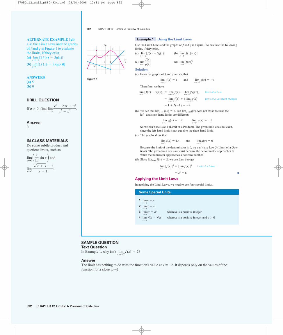
Use the Limit Laws and the graphs of f and g in Figure 1 to evaluate the followinglimits, if they exist.
(a) (b)
(c) (d)
Solution
(a) From the graphs of f and g we see that
Therefore, we have
Limit of a Sum
Limit of a Constant Multiple
(b) We see that . But does not exist because the left- and right-hand limits are different:
So we can’t use Law 4 (Limit of a Product). The given limit does not exist,since the left-hand limit is not equal to the right-hand limit.
(c) The graphs show that
Because the limit of the denominator is 0, we can’t use Law 5 (Limit of a Quo-tient). The given limit does not exist because the denominator approaches 0while the numerator approaches a nonzero number.
(d) Since , we use Law 6 to get
Limit of a Power
■
Applying the Limit Laws
In applying the Limit Laws, we need to use four special limits.
� 23 � 8
limx�13f 1x 2 4 3 � 3 lim
x�1 f 1x 2 4 3limxS1 f 1x 2 � 2
limx�2
f 1x 2 � 1.4 and limx�2
g1x 2 � 0
limx�1�
g1x 2 � �2 limx�1�
g1x 2 � �1
limxS1 g1x 2limxS1 f 1x 2 � 2
� 1 � 51�1 2 � �4
� limx��2
f 1x 2 � 5 limx��2
g1x 2 limx��23f 1x 2 � 5g1x 2 4 � lim
x��2f 1x 2 � lim
x��235g1x 2 4
limx��2
f 1x 2 � 1 and limx��2
g1x 2 � �1
limx�13f 1x 2 4 3lim
x�2 f 1x 2g1x 2
limx�13f 1x 2g1x 2 4lim
x��23f 1x 2 � 5g1x 2 4
892 CHAPTER 12 Limits: A Preview of Calculus
0
f
g1
1
y
x
Figure 1
Some Special Units
1.
2.
3. where n is a positive integer
4. where n is a positive integer and a � 0limx�a
1n x � 1n a
limx�a
xn � an
limx�a
x � a
limx�a
c � c
57050_12_ch12_p880-934.qxd 08/04/2008 12:31 PM Page 892

CHAPTER 12 Limits: A Preview of Calculus 893
ALTERNATE EXAMPLE 2aEvaluate the limit:
ANSWER 31
limx: -2
(6x2 - 3x + 1).
EXAMPLESAlgebraic simplification:
■
■ does not exist
■ by direct substitutionlimx:0
x - 2
x2 + x - 6=
1
3
limx:3
x - 2
x2 + x - 6
limx:2
x - 2
x2 + x - 6=
1
5
Special Limits 1 and 2 are intuitively obvious—looking at the graphs of y � c and y � x will convince you of their validity. Limits 3 and 4 are special cases of LimitLaws 6 and 7 (Limits of a Power and of a Root).
Example 2 Using the Limit Laws
Evaluate the following limits and justify each step.
(a) (b)
Solution
(a) Limits of a Difference and SumLimit of a Constant Multiple
Special Limits 3, 2, and 1
(b) We start by using Law 5, but its use is fully justified only at the final stagewhen we see that the limits of the numerator and denominator exist and thelimit of the denominator is not 0.
Limit of a Quotient
Special Limits 3, 2, and 1
■
If we let , then . In Example 2(a), we found that. In other words, we would have gotten the correct answer by sub-
stituting 5 for x. Similarly, direct substitution provides the correct answer in part (b).The functions in Example 2 are a polynomial and a rational function, respectively,and similar use of the Limit Laws proves that direct substitution always works forsuch functions. We state this fact as follows.
limxS5 f 1x 2 � 39f 15 2 � 39f 1x 2 � 2x2 � 3x � 4
� �
1
11
� 1�2 2 3 � 21�2 2 2 � 1
5 � 31�2 2Limits of Sums, Differ-ences, and ConstantMultiples
� lim
x��2x3 � 2 lim
x��2x2 � lim
x��21
limx��2
5 � 3 limx��2
x
limx��2
x3 � 2x2 � 1
5 � 3x�
limx��21x3 � 2x2 � 1 2
limx��215 � 3x 2
� 39
� 2152 2 � 315 2 � 4
� 2 limx�5
x2 � 3 limx�5
x � limx�5
4
limx�5 12x2 � 3x � 4 2 � lim
x�512x2 2 � lim
x�513x 2 � lim
x�5 4
limx��2
x3 � 2x2 � 1
5 � 3xlimx�5 12x2 � 3x � 4 2
SECTION 12.2 Finding Limits Algebraically 893
Limits by Direct Substitution
If f is a polynomial or a rational function and a is in the domain of f, then
limx�a
f 1x 2 � f 1a 2Functions with this direct substitution property are called continuous at a. You
will learn more about continuous functions when you study calculus.
57050_12_ch12_p880-934.qxd 08/04/2008 12:31 PM Page 893

894 CHAPTER 12 Limits: A Preview of Calculus
ALTERNATE EXAMPLE 3bEvaluate the limit:
.
ANSWER
ALTERNATE EXAMPLE 4
Find
ANSWER1
8
limx:4
x - 4
x2 - 16
.
16
19
limx:2
x2 + 6x
x4
+ 3
Example 3 Finding Limits by Direct Substitution
Evaluate the following limits.
(a) (b)
Solution
(a) The function is a polynomial, so we can find the limitby direct substitution:
(b) The function is a rational function, and x � �1 isin its domain (because the denominator is not zero for x � �1). Thus, we canfind the limit by direct substitution:
■
Finding Limits Using Algebra and the Limit Laws
As we saw in Example 3, evaluating limits by direct substitution is easy. But not alllimits can be evaluated this way. In fact, most of the situations in which limits are use-ful requires us to work harder to evaluate the limit. The next three examples illustratehow we can use algebra to find limits.
Example 4 Finding a Limit by Canceling a Common Factor
Find .
Solution Let . We can’t find the limit by substituting x � 1 because isn’t defined. Nor can we apply Law 5 (Limit of a Quotient) because the limit of the denominator is 0. Instead, we need to do some preliminaryalgebra. We factor the denominator as a difference of squares:
The numerator and denominator have a common factor of x � 1. When we take thelimit as x approaches 1, we have x � 1 and so x � 1 � 0. Therefore, we can cancelthe common factor and compute the limit as follows:
Factor
Cancel
Let x � 1
This calculation confirms algebraically the answer we got numerically andgraphically in Example 1 in Section 12.1. ■
� 1
1 � 1�
1
2
� limx�1
1
x � 1
limx�1
x � 1
x2 � 1� lim
x�1
x � 11x � 1 2 1x � 1 2
x � 1
x2 � 1�
x � 11x � 1 2 1x � 1 2f 11 2f 1x 2 � 1x � 1 2/ 1x2 � 1 2lim
x�1
x � 1
x2 � 1
limx��1
x2 � 5x
x4 � 2�1�1 2 2 � 51�1 21�1 2 4 � 2
� �
4
3
f 1x 2 � 1x2 � 5x 2 / 1x4 � 2 2limx�3
12x3 � 10x � 12 2 � 213 2 3 � 1013 2 � 8 � 16
f 1x 2 � 2x3 � 10x � 12
limx��1
x2 � 5x
x4 � 2limx�312x3 � 10x � 8 2
894 CHAPTER 12 Limits: A Preview of Calculus
Sir Isaac Newton (1642–1727) isuniversally regarded as one of thegiants of physics and mathematics.He is well known for discoveringthe laws of motion and gravity andfor inventing the calculus, but healso proved the Binomial Theoremand the laws of optics, and devel-oped methods for solving poly-nomial equations to any desiredaccuracy. He was born on Christ-mas Day, a few months after thedeath of his father. After an un-happy childhood, he entered Cam-bridge University, where he learnedmathematics by studying the writ-ings of Euclid and Descartes.
During the plague years of1665 and 1666, when the univer-sity was closed, Newton thoughtand wrote about ideas that, oncepublished, instantly revolutionizedthe sciences. Imbued with a patho-logical fear of criticism, he pub-lished these writings only aftermany years of encouragementfrom Edmund Halley (who discov-ered the now-famous comet) andother colleagues.
Newton’s works brought himenormous fame and prestige. Evenpoets were moved to praise;Alexander Pope wrote:
Nature and Nature’s Lawslay hid in Night.
God said, “Let Newton be”and all was Light.
(continued )
Bill
Sane
ders
on/S
PL/P
hoto
Res
earc
hers
, Inc
.
57050_12_ch12_p880-934.qxd 08/04/2008 12:31 PM Page 894

CHAPTER 12 Limits: A Preview of Calculus 895
ALTERNATE EXAMPLE 5
Evaluate
ANSWER 8
ALTERNATE EXAMPLE 6
Find .
ANSWER
IN-CLASS MATERIALS
Compute some limits of quotients,
such as , ,
, and ,
always attempting to plug valuesin first.
limx:2
x3 - 8
x - 2limx:3
x3 - 8
x - 2
limx:0
x3 - 8
x - 2limx:2
x2 - 4
x - 2
1
2
limx:1
2x - 1
x - 1
limh:0
(4 + h)2 - 16
h.
EXAMPLEAlgebraic simplification, with variables:This limit will be seen again in calculus, and provides a good review of the algebra involved in workingwith fractions.
limh:0
1
x + h-
1x
h= lim
h:0
x - (x + h)
x(x + h)
h= lim
h:0
x - (x + h)
hx(x + h)1 = lim
h:0 -
1
x(x + h)= -
1
x2
Example 5 Finding a Limit by Simplifying
Evaluate .
Solution We can’t use direct substitution to evaluate this limit, because the limitof the denominator is 0. So we first simplify the limit algebraically.
Expand
Simplify
Cancel h
Let h � 0 ■
Example 6 Finding a Limit by Rationalizing
Find .
Solution We can’t apply Law 5 (Limit of a Quotient) immediately, since thelimit of the denominator is 0. Here the preliminary algebra consists of rationalizingthe numerator:
Rationalize numerator
This calculation confirms the guess that we made in Example 2 in Section 12.1. ■
Using Left- and Right-Hand Limits
Some limits are best calculated by first finding the left- and right-hand limits. The following theorem is a reminder of what we discovered in Section 12.1. It says that a two-sided limit exists if and only if both of the one-sided limits exist and are equal.
When computing one-sided limits, we use the fact that the Limit Laws also holdfor one-sided limits.
� limt�0
1
2t2 � 9 � 3�
1
2limt�01t2 � 9 2 � 3
�1
3 � 3�
1
6
� limt�0
1t2 � 9 2 � 9
t2A2t2 � 9 � 3B � limt�0
t2
t2A2t2 � 9 � 3B limt�0
2t2 � 9 � 3
t2 � limt�0
2t2 � 9 � 3
t2# 2t2 � 9 � 3
2t2 � 9 � 3
limt�0
2t2 � 9 � 3
t2
� 6
� limh�016 � h 2 � lim
h�0 6h � h2
h
limh�0
13 � h 2 2 � 9
h� lim
h�0 19 � 6h � h2 2 � 9
h
limh�0
13 � h 2 2 � 9
h
SECTION 12.2 Finding Limits Algebraically 895
limx�a
f 1x 2 � L if and only if limx�a�
f 1x 2 � L � limx�a�
f 1x 2
Newton was far more modestabout his accomplishments. Hesaid, “I seem to have been only likea boy playing on the seashore . . .while the great ocean of truth layall undiscovered before me.” New-ton was knighted by Queen Annein 1705 and was buried with greathonor in Westminster Abbey.
57050_12_ch12_p880-934.qxd 08/04/2008 12:31 PM Page 895
896 CHAPTER 12 Limits: A Preview of Calculus
ALTERNATE EXAMPLE 7
Find
ANSWER 0
IN-CLASS MATERIALS
Have students determine theexistence of and
determine why we cannot
compute .
ALTERNATE EXAMPLE 8
Find
ANSWER No solution
ALTERNATE EXAMPLE 9Find if:
ANSWER 0
f (x) = e1x - 7 if x 7 7
28 - 4x if x 6 7
limx:7
f (x)
limz:0
|2z|
2z.
limx:0 1x
limx:0 +
1x
limt:0
ƒ t ƒ .
IN-CLASS MATERIALS
Have students check if exists, and then compute left- and right-hand limits. Then check
limx: -5
(x + 5)2
| x + 5 |.
limx: -5
x + 5
| x + 5 |
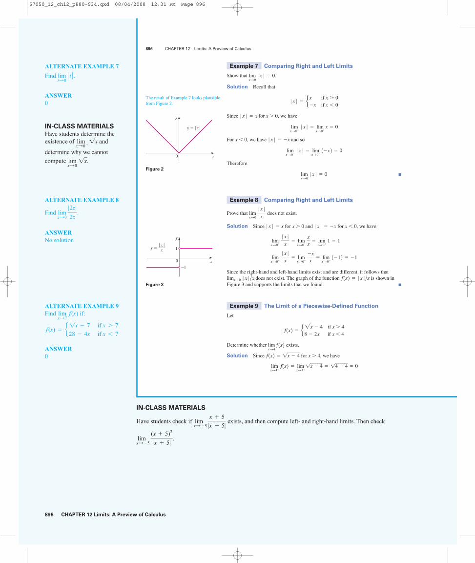
Example 7 Comparing Right and Left Limits
Show that .
Solution Recall that
Since for x � 0, we have
For x � 0, we have and so
Therefore
■
Example 8 Comparing Right and Left Limits
Prove that does not exist.
Solution Since for x � 0 and for x � 0, we have
Since the right-hand and left-hand limits exist and are different, it follows thatdoes not exist. The graph of the function is shown in
Figure 3 and supports the limits that we found. ■
Example 9 The Limit of a Piecewise-Defined Function
Let
if x � 4
if x � 4
Determine whether exists.
Solution Since for x � 4, we have
limx�4�
f1x 2 � limx�4�1x � 4 � 14 � 4 � 0
f 1x 2 � 1x � 4
limx�4
f 1x 2f 1x 2 � e2x � 4
8 � 2x
f 1x 2 � 0 x 0 /xlimx�0 0 x 0 /x
limx�0�
0 x 0x
� limx�0�
�xx
� limx�0�
1�1 2 � �1
limx�0�
0 x 0x
� limx�0�
xx
� limx�0�
1 � 1
0 x 0 � �x0 x 0 � x
limx�0
0 x 0x
limx�0
0 x 0 � 0
limx�0�
0 x 0 � limx�0�
1�x 2 � 0
0 x 0 � �x
limx�0�
0 x 0 � limx�0�
x � 0
0 x 0 � x
0 x 0 � e x if x � 0
�x if x � 0
limx�00 x 0 � 0
896 CHAPTER 12 Limits: A Preview of Calculus
0
y=|x|
y
x
Figure 2
1
_10
y=|x|x
y
x
Figure 3
The result of Example 7 looks plausiblefrom Figure 2.
57050_12_ch12_p880-934.qxd 08/04/2008 12:31 PM Page 896

CHAPTER 12 Limits: A Preview of Calculus 897
Since for x � 4, we have
The right- and left-hand limits are equal. Thus, the limit exists and
The graph of f is shown in Figure 4. ■
12.2 Exercises
limx�4
f 1x 2 � 0
limx�4�
f 1x 2 � limx�4�18 � 2x 2 � 8 � 2 # 4 � 0
f 1x 2 � 8 � 2x
SECTION 12.2 Finding Limits Algebraically 897
40
y
x
Figure 4
1. Suppose that
Find the value of the given limit. If the limit does not exist,explain why.
(a) (b)
(c) (d)
(e) (f)
(g) (h)
2. The graphs of f and g are given. Use them to evaluate eachlimit, if it exists. If the limit does not exist, explain why.
(a) (b)
(c) (d)
(e) (f)
3–8 ■ Evaluate the limit and justify each step by indicating theappropriate Limit Law(s).
3. 4.
5. 6.
7. 8. limu��2
2u4 � 3u � 6limt��21t � 1 2 91t2 � 1 2 lim
x�1a x4 � x2 � 6
x4 � 2x � 3b 2
limx��1
x � 2
x2 � 4x � 3
limx�31x3 � 2 2 1x2 � 5x 2lim
x�415x2 � 2x � 3 2
1
y=Ï1
0 1
y=˝1
y
x x
y
limx�123 � f 1x 2lim
x�2 x
3f 1x 2lim
x��1 f 1x 2g1x 2lim
x�0 3f 1x 2g1x 2 4
limx�1 3f 1x 2 � g1x 2 4lim
x�2 3f 1x 2 � g1x 2 4
limx�a
2f 1x 2
h1x 2 � f 1x 2limx�a
f 1x 2g1x 2
lim x�a
g1x 2f 1x 2lim
x�a f 1x 2h1x 2
limx�a
1
f 1x 2limxSa
13 h1x 2limx�a 3f 1x 2 4 2lim
x�a 3f 1x 2 � h1x 2 4
limx�a
f 1x 2 � �3 limx�a
g1x 2 � 0 limx�a
h1x 2 � 89–20 ■ Evaluate the limit, if it exists.
9. 10.
11. 12.
13. 14.
15. 16.
17. 18.
19. 20.
21–24 ■ Find the limit and use a graphing device to confirmyour result graphically.
21. 22.
23. 24.
25. (a) Estimate the value of
by graphing the function .
(b) Make a table of values of for x close to 0 and guessthe value of the limit.
(c) Use the Limit Laws to prove that your guess is correct.
26. (a) Use a graph of
to estimate the value of to two decimalplaces.
limxS0 f 1x 2f 1x 2 �
23 � x � 13x
f 1x 2f 1x 2 � x/ A11 � 3x � 1Blimx�0
x
21 � 3x � 1
limx�1
x8 � 1
x5 � xlim
x��1
x2 � x � 2
x3 � x
limx�0
14 � x 2 3 � 64
xlimx�1
x2 � 1
1x � 1
limt�0a 1
t�
1
t2 � tblim
x��4
1
4�
1x
4 � x
limh�0
13 � h 2�1 � 3�1
hlimx�7
1x � 2 � 3
x � 7
limx�2
x4 � 16
x � 2limh�0
12 � h 2 3 � 8
h
limh�0
11 � h � 1
hlim
t��3
t2 � 9
2t2 � 7t � 3
limx�1
x3 � 1
x2 � 1limx�2
x2 � x � 6
x � 2
limx��4
x2 � 5x � 4
x2 � 3x � 4limx�2
x2 � x � 6
x � 2
57050_12_ch12_p880-934.qxd 08/04/2008 12:31 PM Page 897

898 CHAPTER 12 Limits: A Preview of Calculus
SUGGESTED TIME
AND EMPHASIS
1–2 classes. Optional material.
POINTS TO STRESS
1. Definition of a tangent line.2. Definition of the slope of a curve.3. Definition of the derivative.4. The difference between average and instantaneous rates of change.
898 CHAPTER 12 Limits: A Preview of Calculus
(b) Use a table of values of to estimate the limit tofour decimal places.
(c) Use the Limit Laws to find the exact value of the limit.
27–32 ■ Find the limit, if it exists. If the limit does not exist,explain why.
27. 28.
29. 30.
31. 32.
33. Let
(a) Find .
(b) Does exist?
(c) Sketch the graph of f.
34. Let
(a) Evaluate each limit, if it exists.
(i) (iv)
(ii) (v)
(iii) (vi)
(b) Sketch the graph of h.
limx�2
h1x 2limx�1
h1x 2 limx�2�
h1x 2limx�0
h1x 2 limx�2�
h1x 2limx�0�
h1x 2h1x 2 � • x if x � 0
x2 if 0 � x 2
8 � x if x � 2
limx�2 f 1x 2limxS2� f 1x 2 and limxS2� f 1x 2f1x 2 � e x � 1 if x � 2
x2 � 4x � 6 if x � 2
limx�0�a 1
x�
10 x 0 blimx�0�a 1
x�
10 x 0 blim
x�1.5 2x2 � 3x0 2x � 3 0lim
x�2 0 x � 2 0x � 2
limx��4�
0 x � 4 0x � 4
limx��4
0 x � 4 0
f 1x 2 Discovery • Discussion
35. Cancellation and Limits
(a) What is wrong with the following equation?
(b) In view of part (a), explain why the equation
is correct.
36. The Lorentz Contraction In the theory of relativity, theLorentz contraction formula
expresses the length L of an object as a function of its velocity √ with respect to an observer, where L0 is thelength of the object at rest and c is the speed of light. Find
L and interpret the result. Why is a left-hand limitnecessary?
37. Limits of Sums and Products
(a) Show by means of an example thatmay exist even though neither
exists.
(b) Show by means of an example thatmay exist even though neither
exists.limx�a f 1x 2 nor limx�a g1x 2limx�a 3f 1x 2g1x 2 4limx�a f 1x 2 nor limx�a g1x 2limx�a 3f 1x 2 � g1x 2 4
lim√Sc�
L � L021 � √ 2/c2
limx�2
x2 � x � 6
x � 2� lim
x�2 1x � 3 2
x2 � x � 6
x � 2� x � 3
12.3 Tangent Lines and Derivatives
In this section we see how limits arise when we attempt to find the tangent line to acurve or the instantaneous rate of change of a function.
The Tangent Problem
A tangent line is a line that just touches a curve. For instance, Figure 1 shows theparabola y � x 2 and the tangent line t that touches the parabola at the point .We will be able to find an equation of the tangent line t as soon as we know its slopem. The difficulty is that we know only one point, P, on t, whereas we need two pointsto compute the slope. But observe that we can compute an approximation to m by
P11, 1 20
y=≈
t
P (1, 1)
y
x
Figure 1
57050_12_ch12_p880-934.qxd 08/04/2008 12:31 PM Page 898

CHAPTER 12 Limits: A Preview of Calculus 899
choosing a nearby point on the parabola (as in Figure 2) and computing theslope mPQ of the secant line PQ.
We choose x � 1 so that Q � P. Then
Now we let x approach 1, so Q approaches P along the parabola. Figure 3 shows howthe corresponding secant lines rotate about P and approach the tangent line t.
Figure 3
The slope of the tangent line is the limit of the slopes of the secant lines:
So, using the method of Section 12.2, we have
Now that we know the slope of the tangent line is m � 2, we can use the point-slopeform of the equation of a line to find its equation:
y � 1 � 21x � 1 2 or y � 2x � 1
� limx�1 1x � 1 2 � 1 � 1 � 2
m � limx�1
x2 � 1
x � 1� lim
x�1 1x � 1 2 1x � 1 2
x � 1
m � limQ�P
mPQ
Q approaches P from the right
P
0
Q
t
Q approaches P from the left
P
0
Qt
P
0
Q
t
P
0
Q
t
P
0
Q
t
P
0Q
t
y
x
y
x
y
x
y
x
y
x
y
x
mPQ �x2 � 1
x � 1
Q1x, x2 2SECTION 12.3 Tangent Lines and Derivatives 899
0
y=≈
tQÓx, ≈Ô
P (1, 1)
y
x
Figure 2
The point-slope form for the equationof a line through the point withslope m is
(See Section 1.10.)
y � y1 � m1x � x1 21x1, y1 2
57050_12_ch12_p880-934.qxd 08/04/2008 12:31 PM Page 899

900 CHAPTER 12 Limits: A Preview of Calculus
DRILL QUESTION
Draw the line tangent to thefollowing curve at each of theindicated points:
Answer
SAMPLE QUESTION
Text Question
Geometrically, what is “the line tangent to a curve” at a particular point?
Answer
There are different correct answers. Examples include the best linear approximation to a curve at a point, or the result of repeated “zooming in” on a curve.
We sometimes refer to the slope of the tangent line to a curve at a point as the slopeof the curve at the point. The idea is that if we zoom in far enough toward the point,the curve looks almost like a straight line. Figure 4 illustrates this procedure for thecurve y � x 2. The more we zoom in, the more the parabola looks like a line. In otherwords, the curve becomes almost indistinguishable from its tangent line.
Figure 4
Zooming in toward the point on the parabola y � x 2
If we have a general curve C with equation and we want to find the tan-gent line to C at the point , then we consider a nearby point ,where x � a, and compute the slope of the secant line PQ:
Then we let Q approach P along the curve C by letting x approach a. If mPQ
approaches a number m, then we define the tangent t to be the line through P withslope m. (This amounts to saying that the tangent line is the limiting position of thesecant line PQ as Q approaches P. See Figure 5.)
Figure 5
0
P
tQ
Q
Q
0 a x
PÓa, f(a)ÔÏ- f(a)
x-a
QÓx, ÏÔ
y
x
y
x
mPQ �f 1x 2 � f 1a 2
x � a
Q1x, f 1x 22P1a, f 1a 22 y � f 1x 211, 1 2
(1, 1)
2
0 2
(1, 1)
1.5
0.5 1.5
(1, 1)
1.1
0.9 1.1
900 CHAPTER 12 Limits: A Preview of Calculus
Definition of a Tangent Line
The tangent line to the curve at the point is the linethrough P with slope
provided that this limit exists.
m � limx�a
f 1x 2 � f 1a 2
x � a
P1a, f 1a 22y � f 1x 2
y
y=f(x)
x
y
y=f(x)
x
57050_12_ch12_p880-934.qxd 08/04/2008 12:31 PM Page 900

CHAPTER 12 Limits: A Preview of Calculus 901
ALTERNATE EXAMPLE 1Find an equation of the tangent
line to the hyperbola at thepoint (4, 1).
ANSWER x + 4y - 8 = 0
EXAMPLEIf f(x) = 3x + 4, then f(2) = 3.In fact, f(k) = 3.
y =4x
EXAMPLELet f(x) = x3. Then an equation of the line tangent to this curve at is .y =
3
4 x -
1
4x =
1
2
_1
1
2
3
_1 10
y
x
Example 1 Finding a Tangent Line to a Hyperbola
Find an equation of the tangent line to the hyperbola y � 3/x at the point .
Solution Let . Then the slope of the tangent line at is
Definition of m
Cancel x � 3
Let x � 3
Therefore, an equation of the tangent at the point is
which simplifies to
The hyperbola and its tangent are shown in Figure 6. ■
There is another expression for the slope of a tangent line that is sometimes easierto use. Let h � x � a. Then x � a � h, so the slope of the secant line PQ is
See Figure 7 where the case h � 0 is illustrated and Q is to the right of P. If it hap-pened that h � 0, however, Q would be to the left of P.
Notice that as x approaches a, h approaches 0 (because h � x � a), and so the ex-pression for the slope of the tangent line becomes
0 a a+h
PÓa, f(a)Ôf(a+h)-f(a)
h
QÓa+h, f(a+h)Ô
ty
x
mPQ �f 1a � h 2 � f 1a 2
h
x � 3y � 6 � 0
y � 1 � � 13 1x � 3 213, 1 2 � �
1
3
� limx�3a�
1xb
Multiply numeratorand denominator by x � lim
x�3
3 � x
x1x � 3 2f 1x 2 �
3x � lim
x�3
3x
� 1
x � 3
m � lim x�3
f 1x 2 � f 13 2x � 3
13, 1 2f 1x 2 � 3/x
13, 1 2SECTION 12.3 Tangent Lines and Derivatives 901
0
(3, 1)
x+3y-6=0 y=3x
y
x
Figure 6
Figure 7
m � limh�0
f 1a � h 2 � f 1a 2
h
57050_12_ch12_p880-934.qxd 08/04/2008 12:31 PM Page 901

902 CHAPTER 12 Limits: A Preview of Calculus
ALTERNATE EXAMPLE 2Find an equation of the tangentline to the curve y = x3 - 2x + 5at the point (1, 5).
ANSWER y = x + 4
IN-CLASS MATERIALS
Point out that if a car is drivingalong a curve, the headlights willpoint along the direction of thetangent line.
IN-CLASS MATERIALS
Illustrate that many functions such as x2 and x - 2 sin x look locally linear, and discuss the relationship ofthis property to the concept of the tangent line. Then pose the question, “What does a secant line to a linearfunction look like?”
Example 2 Finding a Tangent Line
Find an equation of the tangent line to the curve y � x 3 � 2x � 3 at the point .
Solution If , then the slope of the tangent line where a � 1 is
Definition of m
Expand numerator
Simplify
Cancel h
Let h � 0
So an equation of the tangent line at is
■
Derivatives
We have seen that the slope of the tangent line to the curve at the pointcan be written as
It turns out that this expression arises in many other contexts as well, such as findingvelocities and other rates of change. Because this type of limit occurs so widely, it isgiven a special name and notation.
limh�0
f 1a � h 2 � f 1a 2
h
1a, f 1a 22 y � f 1x 2
y � 2 � 11x � 1 2 or y � x � 1
11, 2 2� 1
� limh�0 11 � 3h � h2 2� lim
h�0 h � 3h2 � h3
h
� limh�0
1 � 3h � 3h2 � h3 � 2 � 2h � 3 � 2
h
f 1x 2 � x3 � 2x � 3� limh�0
3 11 � h 2 3 � 211 � h 2 � 3 4 � 313 � 211 2 � 3 4
h
m � limh�0
f 11 � h 2 � f 11 2
h
f 1x 2 � x3 � 2x � 3
11, 2 2
902 CHAPTER 12 Limits: A Preview of Calculus
Definition of a Derivative
The derivative of a function f at a number a, denoted by , is
if this limit exists.
f¿ 1a 2 � limh�0
f 1a � h 2 � f 1a 2
h
f¿ 1a 2
Newton and Limits
In 1687 Isaac Newton (see page894) published his masterpiecePrincipia Mathematica. In thiswork, the greatest scientific treatiseever written, Newton set forth hisversion of calculus and used it toinvestigate mechanics, fluid dy-namics, and wave motion, and toexplain the motion of planets andcomets.
The beginnings of calculus arefound in the calculations of areasand volumes by ancient Greekscholars such as Eudoxus andArchimedes. Although aspects ofthe idea of a limit are implicit intheir “method of exhaustion,” Eu-doxus and Archimedes never ex-plicitly formulated the concept of a limit. Likewise, mathematicianssuch as Cavalieri, Ferinat, and Bar-row, the immediate precursors ofNewton in the development of cal-culus, did not actually use limits. Itwas Isaac Newton who first talkedexplicitly about limits. He ex-plained that the main idea behindlimits is that quantities “approachnearer than by any given differ-ence.” Newton stated that the limitwas the basic concept in calculusbut it was left to later mathemati-cians like Cauchy to clarify theseideas.
57050_12_ch12_p880-934.qxd 08/04/2008 12:31 PM Page 902

CHAPTER 12 Limits: A Preview of Calculus 903
ALTERNATE EXAMPLE 3 Find the derivative of the functionf(x) = 8x2 + 2x - 4 at the number2.
ANSWER 34
ALTERNATE EXAMPLE 4aLet . Find f (a).
ANSWER
ALTERNATE EXAMPLE 4bLet . Find f (16).
ANSWER 1
8
¿f (x) = 1x
7
217a
¿f (x) = 17x
IN-CLASS MATERIALS
Show that the slope of the tangent line does not exist at x = 0 for either of and g(x) = |x |. Notethat f has a tangent line (which is vertical), but g does not (it has a cusp).
f (x) = 31x
Example 3 Finding a Derivative at a Point
Find the derivative of the function at the number 2.
Solution According to the definition of a derivative, with a � 2, we have
Definition of
Expand
Simplify
Cancel h
Let h � 0 ■
We see from the definition of a derivative that the number is the same as theslope of the tangent line to the curve at the point . So the result ofExample 2 shows that the slope of the tangent line to the parabola y � 5x 2 � 3x � 1at the point is .
Example 4 Finding a Derivative
Let .
(a) Find .
(b) Find .
Solution
(a) We use the definition of the derivative at a:
Definition of derivative
Rationalize numerator
Difference of squares
Simplify numerator � limh�0
h
hA1a � h � 1aB � lim
h�0 1a � h 2 � a
hA1a � h � 1aB � lim
h�0 1a � h � 1a
h# 1a � h � 1a
1a � h � 1a
f 1x 2 � 1x � limh�0
1a � h � 1a
h
f¿ 1a 2 � limh� 0
f 1a � h 2 � f 1a 2
h
f¿ 11 2 , f¿ 14 2 , and f¿ 19 2f¿ 1a 2f 1x 2 � 1x
f¿ 12 2 � 2312, 25 2 1a, f 1a 22y � f 1x 2 f¿ 1a 2 � 23
� limh�0123 � 5h 2 � lim
h�0 23h � 5h2
h
� limh�0
20 � 20h � 5h2 � 6 � 3h � 1 � 25
h
f 1x 2 � 5x 2 � 3x � 1 � lim h�0
3512 � h 2 2 � 312 � h 2 � 1 4 � 3512 2 2 � 312 2 � 1 4h
f ¿ 12 2 f¿ 12 2 � lim h�0
f 12 � h 2 � f 12 2h
f 1x 2 � 5x2 � 3x � 1
SECTION 12.3 Tangent Lines and Derivatives 903
57050_12_ch12_p880-934.qxd 08/04/2008 12:31 PM Page 903
904 CHAPTER 12 Limits: A Preview of Calculus
IN-CLASS MATERIALS
Discuss how physical situations can be translated into statements about derivatives. For example, thebudget deficit can be viewed as the derivative of the national debt. Describe the units of derivatives in real-world situations. The budget deficit, for example, is measured in billions of dollars per year. Anotherexample: If s(d) represents the sales figures for a magazine given d dollars of advertising, where s is thenumber of magazines sold, then s (d) is in magazines per dollar spent. Describe enough examples tomake the pattern evident.
¿
Cancel h
Let h � 0
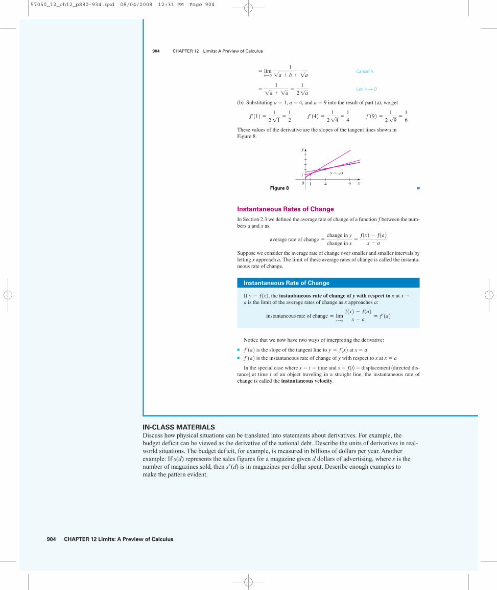
(b) Substituting a � 1, a � 4, and a � 9 into the result of part (a), we get
These values of the derivative are the slopes of the tangent lines shown in Figure 8.
■
Instantaneous Rates of Change
In Section 2.3 we defined the average rate of change of a function f between the num-bers a and x as
Suppose we consider the average rate of change over smaller and smaller intervals byletting x approach a. The limit of these average rates of change is called the instanta-neous rate of change.
average rate of change �change in y
change in x�
f 1x 2 � f 1a 2x � a
941
1
0
y=Ϸx
y
xFigure 8
f¿ 11 2 �1
2 11�
1
2 f¿ 14 2 �
1
2 14�
1
4 f¿ 19 2 �
1
2 19�
1
6
� 1
1a � 1a�
1
2 1a
� limh�0
1
1a � h � 1a
904 CHAPTER 12 Limits: A Preview of Calculus
Instantaneous Rate of Change
If , the instantaneous rate of change of y with respect to x at x �a is the limit of the average rates of change as x approaches a:
instantaneous rate of change � limx�a
f 1x 2 � f 1a 2
x � a� f¿ 1a 2
y � f 1x 2
Notice that we now have two ways of interpreting the derivative:
■ is the slope of the tangent line to at x � a■ is the instantaneous rate of change of y with respect to x at x � a
In the special case where x � t � time and s � f 1t2� displacement 1directed dis-tance2 at time t of an object traveling in a straight line, the instantaneous rate ofchange is called the instantaneous velocity.
f¿ 1a 2 y � f 1x 2f¿ 1a 2
57050_12_ch12_p880-934.qxd 08/04/2008 12:31 PM Page 904

CHAPTER 12 Limits: A Preview of Calculus 905
ALTERNATE EXAMPLE 5If an object is dropped from aheight of 3000 ft, its distanceabove the ground (in feet) after t seconds is given by h(t) = 3000 - 18t2. Find theobject’s instantaneous velocityafter 3 seconds.
ANSWER -108
ALTERNATE EXAMPLE 6Let P(t) be the population of theUnited States at time t. The tablebelow gives approximate values ofthis function by providing midyearpopulation estimates from 1992 to2000. Estimate the value of P (1996).
t P(t)
1992 254,999,000 1994 260,295,000 1996 265,254,000 1998 270,004,000 2000 274,634,000
ANSWER 2.4
¿
IN-CLASS MATERIALS
Show students how to estimate derivatives from tables of numbers. For example, one can estimate that ifthe following are position measurements versus time, the maximum velocity is achieved somewherebetween t = 2.9 and t = 3.
t 2.8 2.9 3.0 3.1 3.2 3.3P(t) 1.2 2.4 3.9 5.1 6.1 6.9
h(t)
Example 5 Instantaneous Velocity
of a Falling Object
If an object is dropped from a height of 3000 ft, its distance above the ground (infeet) after t seconds is given by . Find the object’s instanta-neous velocity after 4 seconds.
Solution After 4 s have elapsed, the height is ft. The instantaneousvelocity is
Definition of
Simplify
Factor numerator
Cancel t � 4
/s Let t � 4
The negative sign indicates that the height is decreasing at a rate of 128 ft/s. ■
Example 6 Estimating an Instantaneous
Rate of Change
Let be the population of the United States at time t. The table in the margingives approximate values of this function by providing midyear population esti-mates from 1996 to 2004. Interpret and estimate the value of .
Solution The derivative means the rate of change of P with respect to twhen t � 2000, that is, the rate of increase of the population in 2000.
According to the definition of a derivative, we have
So we compute and tabulate values of the difference quotient (the average rates ofchange) as shown in the table in the margin. We see that P(2000) lies somewherebetween 3,038,500 and 2,874,500. (Here we are making the reasonable assumptionthat the population didn’t fluctuate wildly between 1996 and 2004.) We estimatethat the rate of increase of the U.S. population in 2000 was the average of these twonumbers, namely
/year ■P¿ 12000 2 � 2.96 million people
P¿ 12000 2 � limt�2000
P1t 2 � P12000 2t � 2000
P¿ 12000 2 P¿ 12000 2P1t 2
� �1614 � 4 2 � �128 ft
� limt�4
�1614 � t 2� limt�4
1614 � t 2 14 � t 2
t � 4
� limt�4
256 � 16t2
t � 4
h1t 2 � 3000 � 16t2� limt�4
3000 � 16t2 � 2744
t � 4
h¿ 14 2h¿ 14 2 � limt�4
h1t 2 � h14 2
t � 4
h14 2 � 2744
h1t 2 � 3000 � 16t2
SECTION 12.3 Tangent Lines and Derivatives 905
h(t)
t
1996 269,667,0001998 276,115,0002000 282,192,0002002 287,941,0002004 293,655,000
P 1t 2
t
1996 3,131,2501998 3,038,5002002 2,874,5002004 2,865,750
P 1t 2 � P 12000 2t � 2000
Here we have estimated the derivativeby averaging the slopes of two secantlines. Another method is to plot thepopulation function and estimate the slope of the tangent line when t � 2000.
57050_12_ch12_p880-934.qxd 08/04/2008 12:32 PM Page 905

906 CHAPTER 12 Limits: A Preview of Calculus
906 CHAPTER 12 Limits: A Preview of Calculus
1–6 ■ Find the slope of the tangent line to the graph of f at thegiven point.
1.
2.
3.
4.
5.
6.
7–12 ■ Find an equation of the tangent line to the curve at thegiven point. Graph the curve and the tangent line.
7.
8.
9.
10.
11.
12.
13–18 ■ Find the derivative of the function at the given number.
13. at 2
14. at �1
15. at 1
16. at 1
17. at 4
18. at 4
19–22 ■ Find , where a is in the domain of f.
19.
20.
21.
22. f 1x 2 � 1x � 2
f 1x 2 �x
x � 1
f 1x 2 � �
1
x2
f 1x 2 � x2 � 2x
f¿ 1a 2G1x 2 � 1 � 21x
F1x 2 �1
1x
g1x 2 � 2x2 � x3
g1x 2 � x4
f 1x 2 � 2 � 3x � x2
f 1x 2 � 1 � 3x2
y � 11 � 2x at 14, 3 2y � 1x � 3 at 11, 2 2y �1
x2 at 1�1, 1 2y �
x
x � 1 at 12, 2 2y � 2x � x3 at 11, 1 2y � x � x2 at 1�1, 0 2
f 1x 2 �6
x � 1 at 12, 2 2f 1x 2 � 2x3 at 12, 16 2f 1x 2 � 1 � 2x � 3x2 at 11, 0 2f 1x 2 � 4x2 � 3x at 1�1, 7 2f 1x 2 � 5 � 2x at 1�3, 11 2f 1x 2 � 3x � 4 at 11, 7 2
23. (a) If , find .
(b) Find equations of the tangent lines to the graph of f at the points whose x-coordinates are 0, 1, and 2.
(c) Graph f and the three tangent lines.
24. (a) If , find .
(b) Find equations of the tangent lines to the graph of g at the points whose x-coordinates are �1, 0,and 1.
(c) Graph g and the three tangent lines.
Applications
25. Velocity of a Ball If a ball is thrown into the air with a velocity of 40 ft/s, its height (in feet) after tseconds is given by y � 40t � 16t 2. Find the velocity when t � 2.
26. Velocity on the Moon If an arrow is shot upward on themoon with a velocity of 58 m/s, its height (in meters) after tseconds is given by H � 58t � 0.83t 2.
(a) Find the velocity of the arrow after one second.
(b) Find the velocity of the arrow when t � a.
(c) At what time t will the arrow hit the moon?
(d) With what velocity will the arrow hit the moon?
27. Velocity of a Particle The displacement s (in meters) ofa particle moving in a straight line is given by the equationof motion s � 4t 3 � 6t � 2, where t is measured in seconds.Find the velocity of the particle s at times t � a, t � 1,t � 2, t � 3.
28. Inflating a Balloon A spherical balloon is being inflated.Find the rate of change of the surface area withrespect to the radius r when r � 2 ft.
29. Temperature Change A roast turkey is taken from anoven when its temperature has reached 185�F and is placedon a table in a room where the temperature is 75�F. Thegraph shows how the temperature of the turkey decreases
AS � 4pr 2B
g¿ 1a 2g1x 2 � 1/ 12x � 1 2f¿ 1a 2f 1x 2 � x3 � 2x � 4
12.3 Exercises
57050_12_ch12_p880-934.qxd 08/04/2008 12:32 PM Page 906

CHAPTER 12 Limits: A Preview of Calculus 907
SECTION 12.3 Tangent Lines and Derivatives 907
and eventually approaches room temperature. By measuringthe slope of the tangent, estimate the rate of change of thetemperature after an hour.
30. Heart Rate A cardiac monitor is used to measure theheart rate of a patient after surgery. It compiles the numberof heartbeats after t minutes. When the data in the table aregraphed, the slope of the tangent line represents the heartrate in beats per minute.
(a) Find the average heart rates (slopes of the secant lines)over the time intervals 340, 424 and 342, 444.
(b) Estimate the patient’s heart rate after 42 minutes by averaging the slopes of these two secant lines.
31. Water Flow A tank holds 1000 gallons of water, whichdrains from the bottom of the tank in half an hour. The values in the table show the volume V of water remaining in the tank (in gallons) after t minutes.
(a) Find the average rates at which water flows from thetank (slopes of secant lines) for the time intervals 310, 154 and 315, 204.
(b) The slope of the tangent line at the point represents the rate at which water is flowing from the tank after 15 minutes. Estimate this rate by averaging the slopes of the secant lines in part (a).
115, 250 2
T (°F)
0
P
30 60 90 120 150
100
200
t(min)
32. World Population Growth The table gives the world’spopulation in the 20th century.
Estimate the rate of population growth in 1920 and in 1980by averaging the slopes of two secant lines.
Discovery • Discussion
33. Estimating Derivatives from a Graph For the functiong whose graph is given, arrange the following numbers inincreasing order and explain your reasoning.
34. Estimating Velocities from a Graph The graph showsthe position function of a car. Use the shape of the graph toexplain your answers to the following questions.
(a) What was the initial velocity of the car?
(b) Was the car going faster at B or at C?
(c) Was the car slowing down or speeding up at A, B,and C?
(d) What happened between D and E?
t
s
A
0
B
CD E
y=˝
1 3 4_1 0 2
1
2
_1
y
x
0 g¿ 1�2 2 g¿ 10 2 g¿ 12 2 g¿ 14 2
t (min) 5 10 15 20 25 30
V (gal) 694 444 250 111 28 0
t (min) 36 38 40 42 44
Heartbeats 2530 2661 2806 2948 3080
Population PopulationYear (in millions) Year (in millions)
1900 1650 1960 30401910 1750 1970 37101920 1860 1980 44501930 2070 1990 52801940 2300 2000 60801950 2560
57050_12_ch12_p880-934.qxd 08/04/2008 12:32 PM Page 907
908 CHAPTER 12 Limits: A Preview of Calculus
SUGGESTED TIME
AND EMPHASIS
1 class. Optional material.
POINTS TO STRESS
1. Limits at infinity.2. Horizontal asymptotes.3. Limits of sequences.
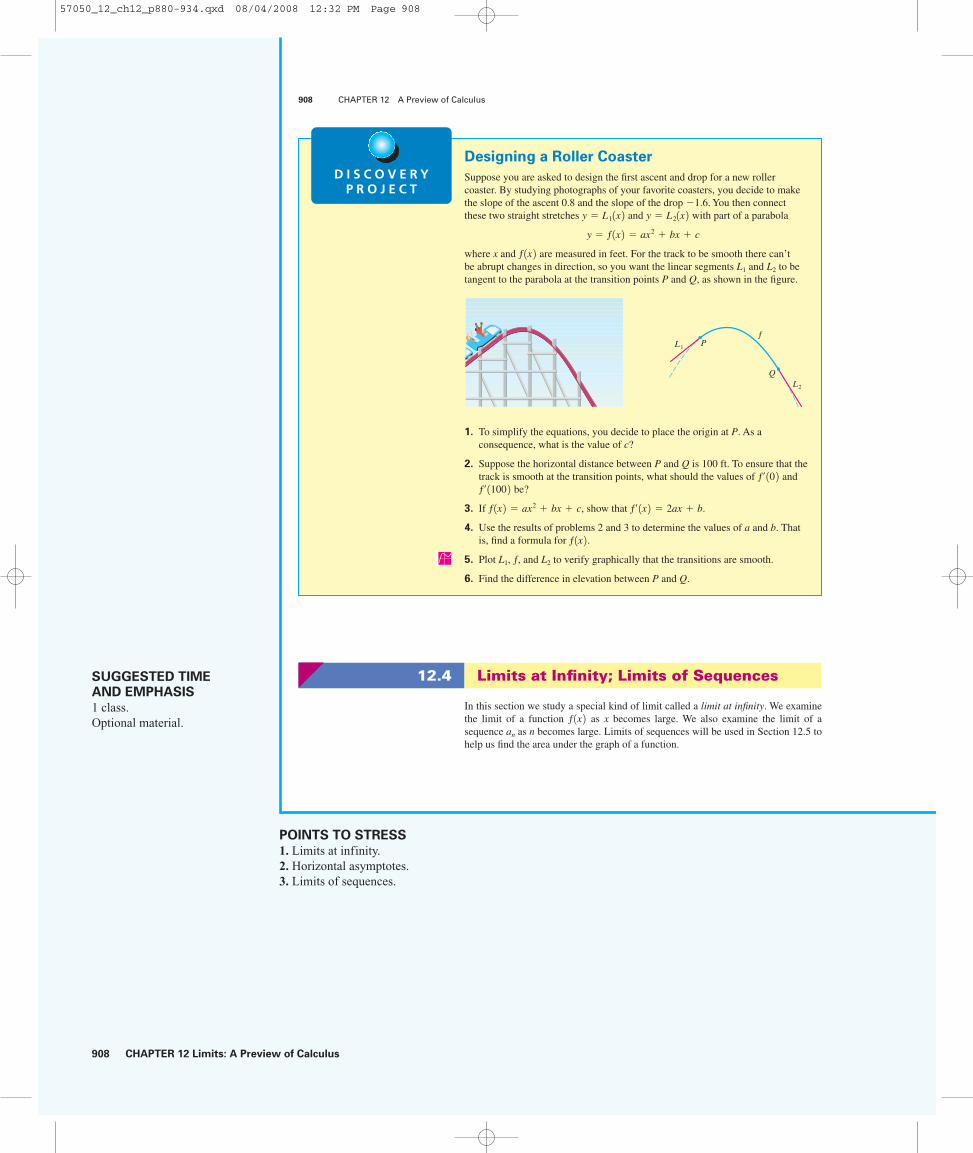
Designing a Roller Coaster
Suppose you are asked to design the first ascent and drop for a new rollercoaster. By studying photographs of your favorite coasters, you decide to makethe slope of the ascent 0.8 and the slope of the drop �1.6. You then connectthese two straight stretches and with part of a parabola
where x and are measured in feet. For the track to be smooth there can’t be abrupt changes in direction, so you want the linear segments L1 and L2 to betangent to the parabola at the transition points P and Q, as shown in the figure.
1. To simplify the equations, you decide to place the origin at P. As a consequence, what is the value of c?
2. Suppose the horizontal distance between P and Q is 100 ft. To ensure that thetrack is smooth at the transition points, what should the values of and
be?
3. If , show that .
4. Use the results of problems 2 and 3 to determine the values of a and b. Thatis, find a formula for .
5. Plot L1, f, and L2 to verify graphically that the transitions are smooth.
6. Find the difference in elevation between P and Q.
f 1x 2f¿ 1x 2 � 2ax � bf 1x 2 � ax2 � bx � c
f¿ 1100 2 f¿ 10 2
L¤
L⁄ Pf
Q
f 1x 2 y � f 1x 2 � ax2 � bx � c
y � L21x 2y � L11x 2
908 CHAPTER 12 A Preview of Calculus
D I S C O V E R YP R O J E C T
12.4 Limits at Infinity; Limits of Sequences
In this section we study a special kind of limit called a limit at infinity. We examinethe limit of a function as x becomes large. We also examine the limit of a sequence an as n becomes large. Limits of sequences will be used in Section 12.5 tohelp us find the area under the graph of a function.
f 1x 2
57050_12_ch12_p880-934.qxd 08/04/2008 12:32 PM Page 908
CHAPTER 12 Limits: A Preview of Calculus 909
SECTION 12.4 Limits at Infinity; Limits of Sequences 909
Limits at Infinity
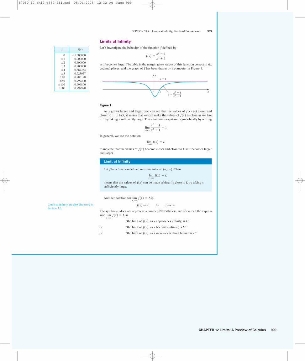
Let’s investigate the behavior of the function f defined by
as x becomes large. The table in the margin gives values of this function correct to sixdecimal places, and the graph of f has been drawn by a computer in Figure 1.
Figure 1
As x grows larger and larger, you can see that the values of get closer andcloser to 1. In fact, it seems that we can make the values of as close as we liketo 1 by taking x sufficiently large. This situation is expressed symbolically by writing
In general, we use the notation
to indicate that the values of become closer and closer to L as x becomes largerand larger.
f 1x 2 limxSq
f 1x 2 � L
limxSq
x2 � 1
x2 � 1� 1
f 1x 2f 1x 210
y=1
y=≈-1≈+1
y
x
f 1x 2 �x2 � 1
x2 � 1
x
0 �1.000000�1 0.000000�2 0.600000�3 0.800000�4 0.882353�5 0.923077
�10 0.980198�50 0.999200
�100 0.999800�1000 0.999998
f 1x 2
Limit at Infinity
Let f be a function defined on some interval . Then
means that the values of can be made arbitrarily close to L by taking xsufficiently large.
f 1x 2 limxSq
f 1x 2 � L
1a, q 2
Another notation for is
The symbol q does not represent a number. Nevertheless, we often read the expres-sion as
“the limit of , as x approaches infinity, is L”
or “the limit of , as x becomes infinite, is L”
or “the limit of , as x increases without bound, is L”f 1x 2f 1x 2f 1x 2limxSq
f 1x 2 � L
f 1x 2 � L as x �q
limxSq
f 1x 2 � L
Limits at infinity are also discussed inSection 3.6.
57050_12_ch12_p880-934.qxd 08/04/2008 12:32 PM Page 909

910 CHAPTER 12 Limits: A Preview of Calculus
IN-CLASS MATERIALS
Consider the motion of an object on a spring. In a frictionless world, it would oscillate forever. In the realworld, the oscillations die out. We can model the height of the object versus time this way:f (x) = e-x sin kx + H where H is the height of the object at rest.
Geometric illustrations are shown in Figure 2. Notice that there are many ways forthe graph of f to approach the line y � L (which is called a horizontal asymptote) aswe look to the far right.
Figure 2
Examples illustrating
Referring back to Figure 1, we see that for numerically large negative values of x,the values of are close to 1. By letting x decrease through negative values with-out bound, we can make as close as we like to 1. This is expressed by writing
The general definition is as follows.
limxS�q
x2 � 1
x2 � 1� 1
f 1x 2f 1x 2limxSq
f 1x 2 � L
0
y=Ï
y=L
0
y=Ï
y=L
0
y=Ï
y=L
y
x
y
x
y
x
910 CHAPTER 12 A Preview of Calculus
Limit at Negative Infinity
Let f be a function defined on some interval . Then
means that the values of can be made arbitrarily close to L by taking xsufficiently large negative.
f 1x 2 limxS�q
f 1x 2 � L
1�q, a 2
Again, the symbol �q does not represent a number, but the expressionis often read as
The definition is illustrated in Figure 3. Notice that the graph approaches the line y � L as we look to the far left.
“the limit of f 1x 2 , as x approaches negative infinity, is L”
limxS�q
f 1x 2 � L
Horizontal Asymptote
The line y � L is called a horizontal asymptote of the curve if either
limxSq
f 1x 2 � L or limxS�q
f 1x 2 � L
y � f 1x 20
y=Ïy=L
0
y=Ï
y=L
y
x
x
y
Figure 3
Examples illustrating limxS�q
f 1x 2 � L
1
2
3
543210
y
x
57050_12_ch12_p880-934.qxd 08/04/2008 12:32 PM Page 910

CHAPTER 12 Limits: A Preview of Calculus 911
SAMPLE QUESTION
Text Question
Compute .
Answer
0
ALTERNATE EXAMPLE 1Find and
.
ANSWER 0, - q
limx: - q
x - 2x2 + 7
limx:q
x - 2x2 + 7
limx:q
1
x2 + 2
IN-CLASS MATERIALS
Note that sometimes we can approximate an infinite limit by shoving large numbers into a function. For
example, let . We can show that , and it is a fact that
. This method doesn’t always work, though. If g(x) = ln(ln x), then ,
that is, the limit does not exist. Yet .g(1099) L 5.4291523
limx:q
g(x) = qf (10)6 L 2.00006
limx:q
f (x) = 2f (x) =2x2 + sin x
x2 - 30x - 200
For instance, the curve illustrated in Figure 1 has the line y � 1 as a horizontal asymptote because
As we discovered in Section 7.4, an example of a curve with two horizontal asymptotes is y � tan�1 x (see Figure 4). In fact,
so both of the lines y � �p/2 and y � p/2 are horizontal asymptotes. (This follows from the fact that the lines x � �p/2 are vertical asymptotes of the graph of tan.)
Example 1 Limits at Infinity
Find .
Solution Observe that when x is large, 1/x is small. For instance,
In fact, by taking x large enough, we can make 1/x as close to 0 as we please.Therefore
Similar reasoning shows that when x is large negative, 1/x is small negative, so wealso have
It follows that the line y � 0 (the x-axis) is a horizontal asymptote of the curve y � 1/x. (This is a hyperbola; see Figure 5.) ■
The Limit Laws that we studied in Section 12.2 also hold for limits at infinity. Inparticular, if we combine Law 6 (Limit of a Power) with the results of Example 1, weobtain the following important rule for calculating limits.
limxS�q
1x
� 0
limxSq
1x
� 0
1
100� 0.01
1
10,000� 0.0001
1
1,000,000� 0.000001
limxSq
1x
and limxS�q
1x
limxS�q
tan�1 x � �
p
2 and lim
xSq tan�1
x �p
2
limxSq
x2 � 1
x2 � 1� 1
SECTION 12.4 Limits at Infinity; Limits of Sequences 911
0
_ π2
π2
x
y
Figure 4
y � tan�1 x
We first investigated horizontal asymptotes and limits at infinity for rational functions in Section 3.6.
0 x
1xy=
y
Figure 5
, limxS�q
1x
� 0limxSq
1x
� 0
If k is any positive integer, then
limxSq
1
xk � 0 and limxS�q
1
xk � 0
57050_12_ch12_p880-934.qxd 08/04/2008 12:32 PM Page 911
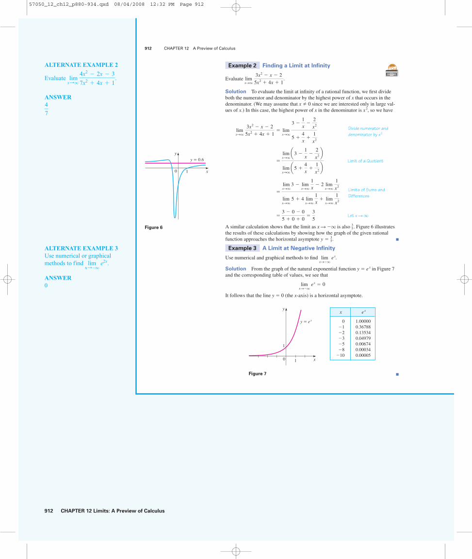
912 CHAPTER 12 Limits: A Preview of Calculus
ALTERNATE EXAMPLE 2
Evaluate .
ANSWER
ALTERNATE EXAMPLE 3 Use numerical or graphicalmethods to find .
ANSWER 0
limx: -q
e2x
4
7
limx:q
4x2 - 2x - 3
7x2 + 4x + 1
Example 2 Finding a Limit at Infinity
Evaluate .
Solution To evaluate the limit at infinity of a rational function, we first divideboth the numerator and denominator by the highest power of x that occurs in thedenominator. (We may assume that x � 0 since we are interested only in large val-ues of x.) In this case, the highest power of x in the denominator is x 2, so we have
Limit of a Quotient
Let x �q
A similar calculation shows that the limit as x �q is also . Figure 6 illustratesthe results of these calculations by showing how the graph of the given rationalfunction approaches the horizontal asymptote . ■
Example 3 A Limit at Negative Infinity
Use numerical and graphical methods to find .
Solution From the graph of the natural exponential function y � ex in Figure 7and the corresponding table of values, we see that
It follows that the line y � 0 (the x-axis) is a horizontal asymptote.
limxS�q
ex � 0
limxS�q
ex
y � 35
35�
� 3 � 0 � 0
5 � 0 � 0�
3
5
Limits of Sums and Differences
�
limxSq
3 � limxSq
1x
� 2 limxSq
1
x2
limxSq
5 � 4 limxSq
1x
� limxSq
1
x2
�
limxSqa3 �
1x
�2
x2 blimxSqa5 �
4x
�1
x2 b
Divide numerator anddenominator by x2
limxSq
3x2 � x � 2
5x2 � 4x � 1� lim
xSq
3 �1x
�2
x2
5 �4x
�1
x2
limxSq
3x2 � x � 2
5x2 � 4x � 1
912 CHAPTER 12 A Preview of Calculus
1
y=0.6
0
y
x
Figure 6
y=Æ
0
1
1
y
x
Figure 7
x ex
0 1.00000�1 0.36788�2 0.13534�3 0.04979�5 0.00674�8 0.00034
�10 0.00005
■
57050_12_ch12_p880-934.qxd 08/04/2008 12:32 PM Page 912

CHAPTER 12 Limits: A Preview of Calculus 913
ALTERNATE EXAMPLE 4
Evaluate .
ANSWER No solution
EXAMPLE
If , then
limx:q
an = 0.
an =n(n + 1)(n + 2)
n4
limx:2
1
x - 2
IN-CLASS MATERIALS
Have the class come up with functions for which both f(x) and an exist, where an = f (n). Then
have them come up with functions for which they both do not exist. Then have them find one where
f(x) does not exist and an does. One such case is f (x) = sin(2px). Finally, have them try to find
an example where an does not exist and f (x) does. They will fail. The text shows that this isimpossible.
limx:q
limx:q
limx:q
limx:q
limx:q
limx:q
Example 4 A Function with No Limit at Infinity
Evaluate .
Solution From the graph in Figure 8 and the periodic nature of the sine function,we see that, as x increases, the values of sin x oscillate between 1 and �1 infinitelyoften and so they don’t approach any definite number. Therefore,does not exist. ■
Limits of Sequences
In Section 11.1 we introduced the idea of a sequence of numbers a1, a2, a3, . . . . Herewe are interested in their behavior as n becomes large. For instance, the sequencedefined by
is pictured in Figure 9 by plotting its terms on a number line and in Figure 10 by plotting its graph. From Figure 9 or 10 it appears that the terms of the sequence
are approaching 1 as n becomes large. We indicate this by writing
limnSq
n
n � 1� 1
an � n/ 1n � 1 2an �
n
n � 1
limxSq sin x
limxSq
sin x
SECTION 12.4 Limits at Infinity; Limits of Sequences 913
0
y=ß xy
x
Figure 8
0 112
a⁄ a¤ a‹a›
Figure 9
0 n
an
1
1
2 3 4 5 6 7
78a‡=
Figure 10
Definition of the Limit of a Sequence
A sequence a1, a2, a3, . . . has the limit L and we write
if the nth term an of the sequence can be made arbitrarily close to L by takingn sufficiently large. If exists, we say the sequence converges (or isconvergent). Otherwise, we say the sequence diverges (or is divergent).
limnSq an
limnSq
an � L or an � L as n �q
This definition is illustrated by Figure 11.
If we compare the definitions of and , we see thatthe only difference is that n is required to be an integer. Thus, the following is true.
limxSq f 1x 2 � LlimnSq an � L
0 n
an
L
1 2 3 0 n
an
L
1 2 3
Figure 11
Graphs of twosequences withlimnSq
an � L
If and when n is an integer, then .limnSq
an � Lf 1n 2 � anlimxSq
f 1x 2 � L
57050_12_ch12_p880-934.qxd 08/04/2008 12:32 PM Page 913

914 CHAPTER 12 Limits: A Preview of Calculus
ALTERNATE EXAMPLE 5
Find .
ANSWER1
ALTERNATE EXAMPLE 6Determine whether the sequencean = 5(-1)n is convergent ordivergent.
ANSWERDivergent
ALTERNATE EXAMPLE 7Find the limit of the sequencegiven by
ANSWER7
DRILL QUESTIONS
(a) Give an example of a diver-gent sequence.
(b) Give an example of asequence whose limit is 2.
Answers
Answers will vary
an =28
n3 cn(n + 4)(2n + 1)
8d .
limn:q
n
n + 4
EXAMPLES
■
■
■ limx:q
x2 - 6x
2x2 + 2x=
1
2
limx:q
1
1 - 21/x = q
limx:q
1
1 - 21/x = -q
In particular, since we know that when k is a positive integer,we have
if k is a positive integer
Note that the Limit Laws given in Section 12.2 also hold for limits of sequences.
Example 5 Finding the Limit of a Sequence
Find .
Solution The method is similar to the one we used in Example 2: Divide the numerator and denominator by the highest power of n and then use the Limit Laws.
Let n �q
Therefore, the sequence is convergent. ■
Example 6 A Sequence That Diverges
Determine whether the sequence is convergent or divergent.
Solution If we write out the terms of the sequence, we obtain
The graph of this sequence is shown in Figure 12. Since the terms oscillate between1 and �1 infinitely often, an does not approach any number. Thus,does not exist; that is, the sequence is divergent. ■
Example 7 Finding the Limit of a Sequence
Find the limit of the sequence given by
Solution Before calculating the limit, let’s first simplify the expression for an.Because n 3 � n # n # n, we place a factor of n beneath each factor in the numeratorthat contains an n:
an �15
6# nn# n � 1
n# 2n � 1
n�
5
2# 1 # a1 �
1nb a2 �
1nb
an �15
n3 c n1n � 1 2 12n � 1 26
d
an � 1�1 2 n limnSq 1�1 2 n�1, 1, �1, 1, �1, 1, �1, . . .
an � 1�1 2 nan � n/ 1n � 1 2 �
1
1 � 0� 1
Limits of a Quotient and a Sum
� limnSq
1
limnSq
1 � limnSq
1n
Divide numerator and denominator by n
limnSq
n
n � 1� lim
nSq
1
1 �1n
limnSq
n
n � 1
limnSq
1
nk � 0
limxSq 11/xk 2 � 0
914 CHAPTER 12 A Preview of Calculus
This result shows that the guess wemade earlier from Figures 9 and 10 was correct.
0 n
an
1
1
2 3 4_1
Figure 12
57050_12_ch12_p880-934.qxd 08/04/2008 12:32 PM Page 914
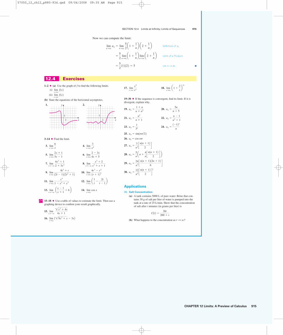
CHAPTER 12 Limits: A Preview of Calculus 915
Now we can compute the limit:
Definition of an
Limit of a Product
Let n �q ■
12.4 Exercises
� 5
2 11 2 12 2 � 5
� 5
2 limnSqa1 �
1nb lim
nSqa2 �
1nb
limnSq
an � limnSq
5
2a1 �
1nb a2 �
1nb
SECTION 12.4 Limits at Infinity; Limits of Sequences 915
1–2 ■ (a) Use the graph of f to find the following limits.
(i)
(ii)
(b) State the equations of the horizontal asymptotes.
1. 2.
3–14 ■ Find the limit.
3. 4.
5. 6.
7. 8.
9. 10.
11. 12.
13. 14.
15–18 ■ Use a table of values to estimate the limit. Then use agraphing device to confirm your result graphically.
15.
16. limxSq
A29x2 � x � 3xBlimxS�q
2x2 � 4x
4x � 1
limxSq
cos xlimxS�q
a x � 1
x � 1� 6 b
limtSq
a 1
t�
2t
t � 1blim
xSq
x4
1 � x2 � x3
limrSq
4r 3 � r 21r � 1 2 3lim
tSq
8t3 � t12t � 1 2 12t2 � 1 2lim
xS�q
x2 � 2
x3 � x � 1lim
xS�q 4x2 � 1
2 � 3x2
limxSq
2 � 3x
4x � 5limxSq
2x � 1
5x � 1
limxSq
3
x4limxSq
6x
1
1
y
x11
x
y
limxSq
f 1x 2limxSq
f 1x 2 17. 18.
19–30 ■ If the sequence is convergent, find its limit. If it is divergent, explain why.
19. 20.
21. 22.
23. 24.
25.
26. an � cos np
27.
28.
29.
30.
Applications
31. Salt Concentration
(a) A tank contains 5000 L of pure water. Brine that con-tains 30 g of salt per liter of water is pumped into thetank at a rate of 25 L/min. Show that the concentrationof salt after t minutes (in grams per liter) is
(b) What happens to the concentration as t q?�
C1t 2 �30t
200 � t
an �12
n4 c n1n � 1 22
d 2an �
24
n3 c n1n � 1 2 12n � 1 26
dan �
5nan �
4nc n1n � 1 2
2d b
an �3
n2 c n1n � 1 22
dan � sin1np/2 2 an �
1�1 2 nn
an �1
3n
an �n � 1
n3 � 1an �
n2
n � 1
an �5n
n � 5an �
1 � n
n � n2
limxSq
a 1 �2xb 3x
limxSq
x5
ex
57050_12_ch12_p880-934.qxd 09/04/2008 09:35 AM Page 915
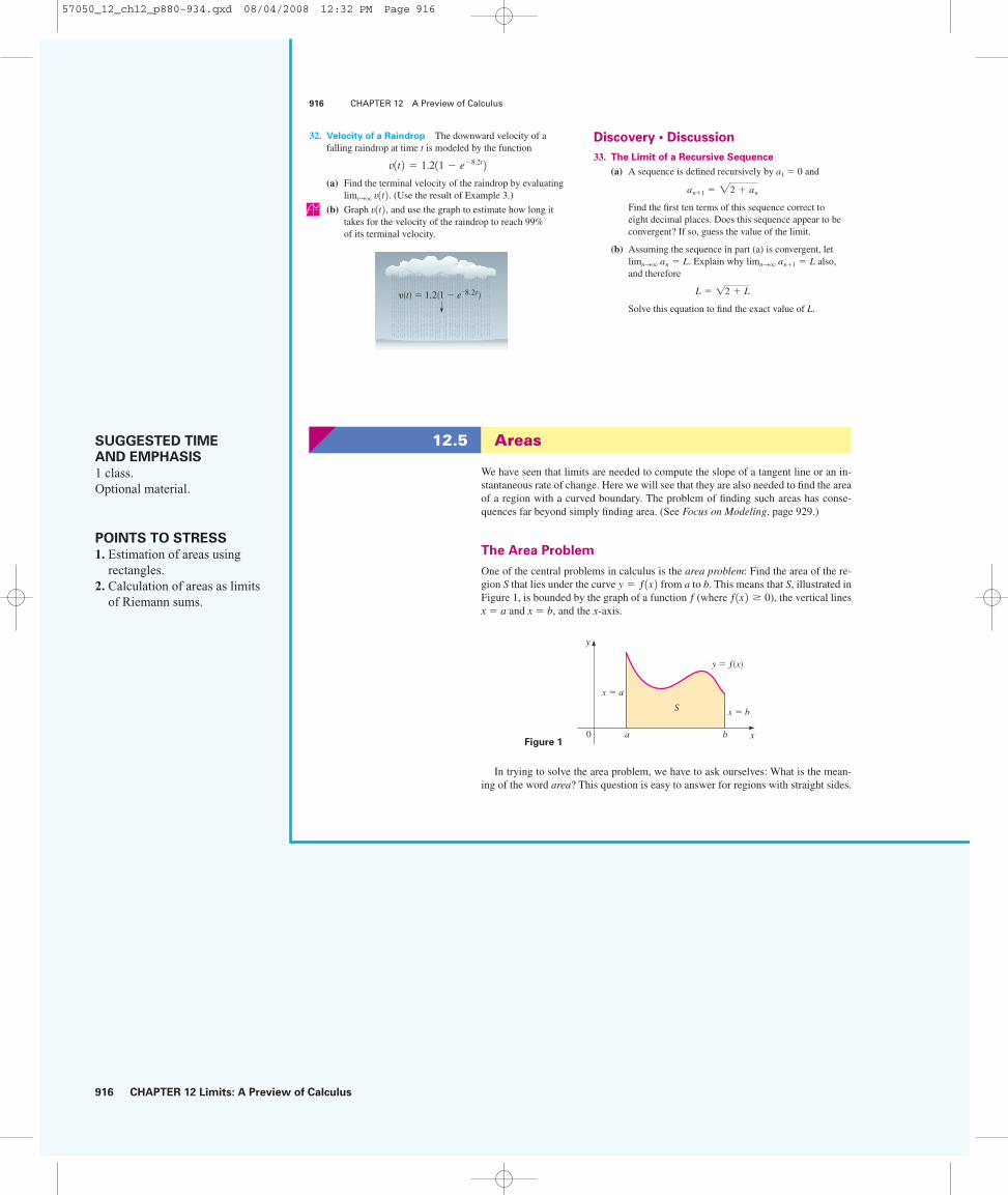
916 CHAPTER 12 Limits: A Preview of Calculus
SUGGESTED TIME
AND EMPHASIS
1 class. Optional material.
POINTS TO STRESS
1. Estimation of areas usingrectangles.
2. Calculation of areas as limitsof Riemann sums.
916 CHAPTER 12 A Preview of Calculus
32. Velocity of a Raindrop The downward velocity of afalling raindrop at time t is modeled by the function
(a) Find the terminal velocity of the raindrop by evaluating. (Use the result of Example 3.)
(b) Graph , and use the graph to estimate how long ittakes for the velocity of the raindrop to reach 99% of its terminal velocity.
�(t)=1.2(1-e–8.2t)
√1t 2limtSq √1t 2√1t 2 � 1.211 � e�8.2t 2 Discovery • Discussion
33. The Limit of a Recursive Sequence
(a) A sequence is defined recursively by a1 � 0 and
Find the first ten terms of this sequence correct to eight decimal places. Does this sequence appear to beconvergent? If so, guess the value of the limit.
(b) Assuming the sequence in part (a) is convergent, let. Explain why also,
and therefore
Solve this equation to find the exact value of L.
L � 12 � L
limnSq an�1 � LlimnSq an � L
an�1 � 22 � an
12.5 Areas
We have seen that limits are needed to compute the slope of a tangent line or an in-stantaneous rate of change. Here we will see that they are also needed to find the areaof a region with a curved boundary. The problem of finding such areas has conse-quences far beyond simply finding area. (See Focus on Modeling, page 929.)
The Area Problem
One of the central problems in calculus is the area problem: Find the area of the re-gion S that lies under the curve from a to b. This means that S, illustrated inFigure 1, is bounded by the graph of a function f (where ), the vertical linesx � a and x � b, and the x-axis.
Figure 1
In trying to solve the area problem, we have to ask ourselves: What is the mean-ing of the word area? This question is easy to answer for regions with straight sides.
0 a b
y=Ï
Sx=a
x=b
y
x
f 1x 2 � 0y � f 1x 2
57050_12_ch12_p880-934.qxd 08/04/2008 12:32 PM Page 916

CHAPTER 12 Limits: A Preview of Calculus 917
ALTERNATE EXAMPLE 1Use four rectangles to estimatethe area under the parabola y = x2
from 0 to 2 (the parabolic region Sillustrated in figure).
ANSWER[1.75, 3.75]
y
4
2
(2, 4)
S
21 x
IN-CLASS MATERIALS
Start by showing how the familiar equation d = rt can be illustrated by a statement about the area of a rectangle (below left). Then assert that wecan generalize this idea by finding the area under a velocity curve to get net distance traveled (below right).
rate varies;distance = shaded area (still)
rate
DISTANCE
r
t time
rate constant;distance = shaded area
rate
DISTANCE
r
timet
For a rectangle, the area is defined as the product of the length and the width. The areaof a triangle is half the base times the height. The area of a polygon is found by di-viding it into triangles (as in Figure 2) and adding the areas of the triangles.
However, it is not so easy to find the area of a region with curved sides. We all havean intuitive idea of what the area of a region is. But part of the area problem is to makethis intuitive idea precise by giving an exact definition of area.
Recall that in defining a tangent we first approximated the slope of the tangent lineby slopes of secant lines and then we took the limit of these approximations. We pur-sue a similar idea for areas. We first approximate the region S by rectangles, and thenwe take the limit of the areas of these rectangles as we increase the number of rec-tangles. The following example illustrates the procedure.
Example 1 Estimating an Area Using Rectangles
Use rectangles to estimate the area under the parabola y � x 2 from 0 to 1 (the para-bolic region S illustrated in Figure 3).
Solution We first notice that the area of S must be somewhere between 0 and 1because S is contained in a square with side length 1, but we can certainly do betterthan that. Suppose we divide S into four strips S1, S2, S3, and S4 by drawing the ver-tical lines as in Figure 4(a). We can approximate each stripby a rectangle whose base is the same as the strip and whose height is the same asthe right edge of the strip (see Figure 4(b)). In other words, the heights of these rectangles are the values of the function at the right endpoints of thesubintervals .30,
14 4 , 3 14,
12 4 , 3 12,
34 4 , and 3 34, 1 4f 1x 2 � x2
x � 14, x � 1
2, and x � 34
A⁄
A¤ A‹
A›
A=A⁄+A¤+A‹+A›
h
b
A= bh12A=l„
l
„
SECTION 12.5 Areas 917
Figure 2
0 1
(1, 1)
y=≈
S
y
x
Figure 3
(a)
0 1
(1, 1)y=≈
34
12
14
S›
S‹S¤S⁄
y
x
Figure 4 (b)
0 134
12
14
(1, 1)y=≈
y
x
57050_12_ch12_p880-934.qxd 08/04/2008 12:32 PM Page 917

918 CHAPTER 12 Limits: A Preview of Calculus
IN-CLASS MATERIALS
Lead students to discover that choosing left endpoints for a decreasing function always leads to anoverestimate, while choosing right endpoints leads to an underestimate. They should check that theopposite trends hold for increasing functions. Challenge them to find a link between the midpoint estimateand the concavity of a graph.
Each rectangle has width and the heights are . If we let R4
be the sum of the areas of these approximating rectangles, we get
From Figure 4(b) we see that the area A of S is less than R4, so
Instead of using the rectangles in Figure 4(b), we could use the smaller rectan-gles in Figure 5 whose heights are the values of f at the left endpoints of the subintervals. (The leftmost rectangle has collapsed because its height is 0.) The sum of the areas of these approximating rectangles is
We see that the area of S is larger than L4, so we have lower and upper estimates for A:
We can repeat this procedure with a larger number of strips. Figure 6 showswhat happens when we divide the region S into eight strips of equal width. By com-puting the sum of the areas of the smaller rectangles and the sum of the areasof the larger rectangles , we obtain better lower and upper estimates for A:
So one possible answer to the question is to say that the true area of S lies some-where between 0.2734375 and 0.3984375.
We could obtain better estimates by increasing the number of strips. The table in the margin shows the results of similar calculations (with a computer) using nrectangles whose heights are found with left endpoints 1Ln2 or right endpoints 1Rn2.In particular, we see by using 50 strips that the area lies between 0.3234 and0.3434. With 1000 strips we narrow it down even more: A lies between 0.3328335and 0.3338335. A good estimate is obtained by averaging these numbers:A � 0.3333335. ■
From the values in the table it looks as if Rn is approaching as n increases. Weconfirm this in the next example.
13
(a) Using left endpoints (b) Using right endpoints
0 118
y=≈(1, 1)
0 118
(1, 1)
y=≈
y
x
y
x
0.2734375 � A � 0.3984375
1R8 2 1L8 20.21875 � A � 0.46875
L4 � 14# 02
� 14# A14B2 � 1
4# A12B2 � 1
4# A34B2 � 7
32 � 0.21875
A � 0.46875
R4 � 14# A14B2 � 1
4# A12B2 � 1
4# A34B2 � 1
4# 12
� 1532 � 0.46875
A14B2, A12B2, A34B2, and 1214
918 CHAPTER 12 A Preview of Calculus
0 1
(1, 1)
34
12
14
y=≈
y
x
Figure 5
Figure 6
Approximating S with eight rectangles
n Ln Rn
10 0.2850000 0.385000020 0.3087500 0.358750030 0.3168519 0.350185250 0.3234000 0.3434000
100 0.3283500 0.33835001000 0.3328335 0.3338335
57050_12_ch12_p880-934.qxd 08/04/2008 12:32 PM Page 918

CHAPTER 12 Limits: A Preview of Calculus 919
ALTERNATE EXAMPLE 2What is the limit of the sum of theupper approximating rectangles?
ANSWER 2
3
1n
0 1
(1, 2)
y=2x2
y
x
Example 2 The Limit of Approximating Sums
For the region S in Example 1, show that the sum of the areas of the upper approximating rectangles approaches , that is,
Solution Rn is the sum of the areas of the n rectangles shown in Figure 7. Eachrectangle has width 1/n, and the heights are the values of the function at the points 1/n, 2/n, 3/n, . . . , n/n. That is, the heights are
. Thus
Here we need the formula for the sum of the squares of the first n positive integers:
Putting the preceding formula into our expression for Rn, we get
Thus, we have
■
It can be shown that the lower approximating sums also approach , that is,
limn�q
Ln � 13
13
� 16 # 1 # 2 � 13
� limn�q
1
6a1 �
1nb a2 �
1nb
� limn�q
1
6a n � 1
nb a 2n � 1
nb
limn�q
Rn � limn�q
1n � 1 2 12n � 1 26n2
Rn �1
n3# n1n � 1 2 12n � 1 2
6�1n � 1 2 12n � 1 2
6n2
12 � 22 � 32 � . . . � n2 �n1n � 1 2 12n � 1 2
6
� 1
n3 112 � 22 � 32 � . . . � n2 2 �
1n# 1n2 112 � 22 � 32 � . . . � n2 2
Rn �1na 1
nb 2
�1na 2
nb 2
�1na 3
nb 2
� . . . �1na n
nb 2
13/n 2 2, . . . , 1n/n 2 2 11/n 2 2, 12/n 2 2,f 1x 2 � x2
limn�q
Rn � 13
13
SECTION 12.5 Areas 919
1n
0 1
(1, 1)
y=≈
y
x
Figure 7
This formula was discussed in Section 11.5.
57050_12_ch12_p880-934.qxd 08/04/2008 12:32 PM Page 919

920 CHAPTER 12 Limits: A Preview of Calculus
IN-CLASS MATERIALS
Look at the function
from x = 0 to
x = 4. Show that the obvious lower and upper bounds for the areaunder the curve are obtained asfollows:
f (x) =6
1 + x2
upper bound
0
1
2
3
4
5
1 2 3
6y
4 x0
1
2
3
4
5
1 2 3
lower bound
6y
4 x
From Figures 8 and 9 it appears that, as n increases, both Rn and Ln become better andbetter approximations to the area of S. Therefore, we define the area A to be the limitof the sums of the areas of the approximating rectangles, that is,
Figure 8
Figure 9
Definition of Area
Let’s apply the idea of Examples 1 and 2 to the more general region S of Figure 1. Westart by subdividing S into n strips S1, S2, . . . , Sn of equal width as in Figure 10.
Figure 100 a bx⁄ x¤ x‹ xi-1 xi xn-1. . .. . .
y=Ï
S⁄ S¤ S‹ Si Sn
y
x
10
n=10 L⁄‚=0.285
10
n=30 L‹‚Å0.3169
10
n=50 Lfi‚=0.3234
y
x
y
x
y
x
10
n=50 Rfi‚=0.3434
10
n=30 R‹‚Å0.3502
10
n=10 R⁄‚=0.385
y
x
y
x
y
x
A � limn�q
Rn � limn�q
Ln � 13
920 CHAPTER 12 A Preview of Calculus
Obtain better lower and upper bounds by dividing the interval into 2 and then4 subintervals. Finally, use the method of counting square units to estimate thearea (between 7 and 8 square units).
57050_12_ch12_p880-934.qxd 08/04/2008 12:32 PM Page 920

CHAPTER 12 Limits: A Preview of Calculus 921
The width of the interval is b � a, so the width of each of the n strips is
These strips divide the interval into n subintervals
where x0 � a and xn � b. The right endpoints of the subintervals are
Let’s approximate the kth strip Sk by a rectangle with width x and height ,which is the value of f at the right endpoint (see Figure 11). Then the area of the kthrectangle is . What we think of intuitively as the area of S is approximated bythe sum of the areas of these rectangles, which is
Figure 12 shows this approximation for n � 2, 4, 8, and 12.
Figure 11
Figure 12
Notice that this approximation appears to become better and better as the numberof strips increases, that is, as n q. Therefore, we define the area A of the region Sin the following way.
�
(a) n=2 (b) n=4 (c) n=8 (d) n=12
0 a bx⁄ 0 a bx⁄ x¤ x‹ 0 a b 0 a b
y
x
y
x
y
x
y
x
0 a bx⁄ x¤ x‹ xk-1 xk
Îx
f(xk)
y
x
Rn � f 1x1 2¢x � f 1x2 2¢x � . . . � f 1xn 2¢x
f 1xk 2¢x
f 1xk 2x1 � a � ¢x, x2 � a � 2 ¢x, x3 � a � 3 ¢x, . . . , xk � a � k ¢x, . . .
3x0, x1 4 , 3x1, x2 4 , 3x2, x3 4 , . . . , 3xn�1, xn 43a, b 4¢x �b � a
n
3a, b 4SECTION 12.5 Areas 921
57050_12_ch12_p880-934.qxd 08/04/2008 12:32 PM Page 921

922 CHAPTER 12 Limits: A Preview of Calculus
SAMPLE QUESTION
Text Question
In the formula
where does
the come from?
Answer
It represents the width of eachrectangle.
ALTERNATE EXAMPLE 3 Find the area of the region thatlies under the parabola
.
ANSWER 512
3
y = x2, 0 … x … 8
¢x
A = limx:qa
n
k = 1f (xk)¢x
EXAMPLESFinding the area under y = sin x from x = 0 to x = p. Note that we get the same results using leftendpoints as we do using right endpoints.
With n = 2 rectangles, our estimate is
With n = 4: A ≈ (1 + ) = 1.8961
With n = 10: A ≈ 1.9835With n = 50: A ≈ 1.9993
12p
4
A Lp
2L 1.5708
In using this formula for area, remember that x is the width of an approximatingrectangle, xk is the right endpoint of the kth rectangle, and is its height. So
When working with sums, we will need the following properties from Section 11.1:
We will also need the following formulas for the sums of the powers of the first nnatural numbers from Section 11.5.
Example 3 Finding the Area under a Curve
Find the area of the region that lies under the parabola y � x 2, 0 x 5.
Solution The region is graphed in Figure 13. To find the area, we first find thedimensions of the approximating rectangles at the nth stage.
Height: f 1xk 2 � f a 5knb � a 5k
nb 2
�25k2
n2
Right endpoint: xk � a � k ¢x � 0 � k a 5nb �
5kn
Width: ¢x �b � a
n�
5 � 0n
�5n
an
k�1k2 �
n1n � 1 2 12n � 1 26
an
k�1k3 �
n21n � 1 2 24
an
k�1c � nc a
n
k�1k �
n1n � 1 22
an
k�11ak � bk 2 � a
n
k�1ak � a
n
k�1bk a
n
k�1cak � ca
n
k�1ak
Height: f 1xk 2 � f 1a � k ¢x 2 Right endpoint: xk � a � k ¢x
Width: ¢x �b � a
n
f 1xk 2
922 CHAPTER 12 A Preview of Calculus
Definition of Area
The area A of the region S that lies under the graph of the continuous func-tion f is the limit of the sum of the areas of approximating rectangles:
Using sigma notation, we write this as follows:
A � limn�q a
n
k�1f 1xk 2¢x
A � limn�q
Rn � limn�q3f 1x1 2¢x � f 1x2 2¢x � . . . � f 1xn 2¢x 4
1 5
5
25
0
y=≈
y
x
Figure 13
57050_12_ch12_p880-934.qxd 08/04/2008 12:32 PM Page 922

CHAPTER 12 Limits: A Preview of Calculus 923
EXAMPLEFinding the area under y = ex
from x = 0 to x = 2:
Estimate Estimateusing left using right
n endpoints endpoints
2 3.7182 10.10734 4.9243 8.1189
10 5.7714 7.049250 6.2621 6.5177
1000 6.3827 6.3954
ALTERNATE EXAMPLE 4Find the area of the region thatlies under the parabola
.
ANSWER148
3
y = 10x - x2, 4 … x … 6
DRILL QUESTION
Estimate the area under y = x2 from x = 1 to x = 3 using two rectangles.Sketch the rectangles you use.
Answer
Answers will vary depending on which rectangles are used.
Now we substitute these values into the definition of area:
Definition of area
Simplify
Factor
Sum of squares formula
Cancel n and expand numerator
Divide numerator and denominator by n2
Let n �q
Thus, the area of the region is . ■
Example 4 Finding the Area under a Curve
Find the area of the region that lies under the parabola y � 4x � x 2, 1 x 3.
Solution We start by finding the dimensions of the approximating rectangles atthe nth stage.
Thus, according to the definition of area, we get
� limn�qa an
k�13 �
4na
n
k�1k �
4
n2 an
k�1k2 b a 2
nb
A � limn�q a
n
k�1f 1xk 2¢x � lim
n�q an
k�1a3 �
4kn
�4k2
n2 b a 2nb
� 3 �4kn
�4k2
n2
� 4 �8kn
� 1 �4kn
�4k2
n2
Height: f 1xk 2 � f a1 �2knb � 4 a1 �
2knb � a1 �
2knb 2
Right endpoint: xk � a � k ¢x � 1 � k a 2nb � 1 �
2kn
Width: ¢x �b � a
n�
3 � 1n
�2n
1253 � 41.7
� 125
6 12 � 0 � 0 2 �
125
3
� limn�q
125
6a2 �
3n
�1
n2 b � lim
n�q
12512n2 � 3n � 1 26n2
� limn�q
125
n3# n1n � 1 2 12n � 1 2
6
125n3 � lim
n�q
125
n3 an
k�1k2
� limn�qa
n
k�1
125k2
n3
f 1xk 2 �25k 2
n2 , ¢x �5n
� limn�q a
n
k�1
25k2
n2# 5n
A � limn�q a
n
k�1f 1xk 2¢x
SECTION 12.5 Areas 923
We can also calculate the limit by writing
as in Example 2.
� 125
6a n
nb a n � 1
nb a 2n � 1
nb
125
n3# n1n � 1 2 12n � 1 2
6
1 40
y=4x-≈
3
y
x
Figure 14
Figure 14 shows the region whose areais computed in Example 4.
57050_12_ch12_p880-934.qxd 08/04/2008 12:32 PM Page 923

924 CHAPTER 12 Limits: A Preview of Calculus
■
12.5 Exercises
� 6 � 4 # 1 �4
3# 1 # 2 �
22
3
� limn�qc6 � 4 a1 �
1nb �
4
3a1 �
1nb a2 �
1nb d
� limn�qa6 � 4 # n
n# n � 1
n�
4
3# nn# n � 1
n# 2n � 1
nb
� limn�qa 2
n 13n 2 �
8
n2 c n1n � 1 22
d �8
n3 c n1n � 1 2 12n � 1 26
d b � lim
n�qa 2
nan
k�13 �
8
n2 an
k�1k �
8
n3 an
k�1k2 b
924 CHAPTER 12 A Preview of Calculus
1. (a) By reading values from the given graph of f, use fiverectangles to find a lower estimate and an upper estimatefor the area under the given graph of f from x � 0 tox � 10. In each case, sketch the rectangles that you use.
(b) Find new estimates using ten rectangles in each case.
2. (a) Use six rectangles to find estimates of each type for thearea under the given graph of f from x � 0 to x � 12.
(i) L6 (using left endpoints)
(ii) R6 (using right endpoints)
(b) Is L6 an underestimate or an overestimate of the truearea?
(c) Is R6 an underestimate or an overestimate of the truearea?
0 4
4
8
y=Ï
8 12
y
x
0 5
5 y=Ï
10
y
x
3–6 ■ Approximate the area of the shaded region under thegraph of the given function by using the indicated rectangles.(The rectangles have equal width.)
3. 4.
5. 6.
7. (a) Estimate the area under the graph of from x � 1 to x � 5 using four approximating rectan-gles and right endpoints. Sketch the graph and the rectangles. Is your estimate an underestimate or anoverestimate?
(b) Repeat part (a) using left endpoints.
f 1x 2 � 1/x
2
5
1
10
0
y
x1
1
70
4
y
x
f 1x 2 � 9x � x3f 1x 2 �4x
1
1
_1 0
y
x1
1
20
y
x
f 1x 2 � 4 � x2f 1x 2 � 12 x � 2
57050_12_ch12_p880-934.qxd 08/04/2008 12:32 PM Page 924

CHAPTER 12 Limits: A Preview of Calculus 925
CHAPTER 12 Review 925
8. (a) Estimate the area under the graph offrom x � 0 to x � 5 using five approximating rectanglesand right endpoints. Sketch the graph and the rectangles.Is your estimate an underestimate or an overestimate?
(b) Repeat part (a) using left endpoints.
9. (a) Estimate the area under the graph of fromx � �1 to x � 2 using three rectangles and right end-points. Then improve your estimate by using six rectan-gles. Sketch the curve and the approximating rectangles.
(b) Repeat part (a) using left endpoints.
10. (a) Estimate the area under the graph of ,0 x 4, using four approximating rectangles andtaking the sample points to be
(i) right endpoints
(ii) left endpoints
In each case, sketch the curve and the rectangles.
(b) Improve your estimates in part (a) by using eight rectangles.
11–12 ■ Use the definition of area as a limit to find the area of the region that lies under the curve. Check your answer bysketching the region and using geometry.
11. y � 3x, 0 x 5 12. y � 2x � 1, 1 x 3
13–18 ■ Find the area of the region that lies under the graph off over the given interval.
13. , 0 x 2
14. , 0 x 1
15. , 0 x 5
16. , 2 x 5
17. , 1 x 4
18. , 2 x 3
Discovery • Discussion
19. Approximating Area with a Calculator When we approximate areas using rectangles as in Example 1, thenthe more rectangles we use the more accurate the answer.
f 1x 2 � 20 � 2x2
f 1x 2 � x � 6x2
f 1x 2 � 4x3
f 1x 2 � x3 � 2
f 1x 2 � x � x2
f 1x 2 � 3x2
f 1x 2 � e�x
f 1x 2 � 1 � x2
f 1x 2 � 25 � x2 The following TI-83 program finds the approximate area under the graph of f on the interval [a, b] using n rectangles.To use the program, first store the function f in Y1. The program prompts you to enter N, the number of rectangles,and A and B, the endpoints of the interval.
(a) Approximate the area under the graph ofon 31, 34 using 10, 20,
and 100 rectangles.
(b) Approximate the area under the graph of f on the giveninterval using 100 rectangles.
(i) , on 30, p4(ii) , on 3�1, 14
PROGRAM:AREA
:Prompt N
:Prompt A
:Prompt B
:(B-A)/N�D
:0�S
:A�X
:For (K,1,N)
:X+D�X
:S+Y1�S
:End
:D*S�S
:Disp "AREA IS"
:Disp S
20. Regions with Straight Versus Curved Boundaries
Write a short essay that explains how you would find the areaof a polygon, that is, a region bounded by straight line seg-ments. Then explain how you would find the area of a regionwhose boundary is curved, as we did in this section. What isthe fundamental difference between these two processes?
f 1x 2 � e�x2
f 1x 2 � sin x
f 1x 2 � x5 � 2x � 3
12 Review
Concept Check
1. Explain in your own words what is meant by the equation
Is it possible for this statement to be true and yet ?Explain.
f 12 2 � 3
limx�2
f 1x 2 � 5
2. Explain what it means to say that
In this situation is it possible that exists? Explain.
limx�1f 1x 2lim
x�1�f 1x 2 � 3 and lim
x�1�f 1x 2 � 7
57050_12_ch12_p880-934.qxd 08/04/2008 12:33 PM Page 925

926 CHAPTER 12 Limits: A Preview of Calculus
926 CHAPTER 12 A Preview of Calculus
3. Describe several ways in which a limit can fail to exist. Illustrate with sketches.
4. State the following Limit Laws.
(a) Sum Law
(b) Difference Law
(c) Constant Multiple Law
(d) Product Law
(e) Quotient Law
(f) Power Law
(g) Root Law
5. Write an expression for the slope of the tangent line to thecurve at the point .
6. Define the derivative . Discuss two ways of interpret-ing this number.
7. If , write expressions for the following.
(a) The average rate of change of y with respect to xbetween the numbers a and x.
(b) The instantaneous rate of change of y with respect to x at x � a.
y � f 1x 2f¿ 1a 2 1a, f 1a 22y � f 1x 2
8. Explain the meaning of the equation
Draw sketches to illustrate the various possibilities.
9. (a) What does it mean to say that the line y � L is a hori-zontal asymptote of the curve ? Draw curves to illustrate the various possibilities.
(b) Which of the following curves have horizontal asymptotes?
(i) y � x 2 (iv) y � tan�1 x
(ii) y � 1/x (v) y � ex
(iii) y � sin x (vi) y � ln x
10. (a) What is a convergent sequence?
(b) What does mean?
11. Suppose S is the region that lies under the graph of.
(a) Explain how this area is approximated using rectangles.
(b) Write an expression for the area of S as a limit of sums.
y � f 1x 2 , a x b
limn�q an � 3
y � f 1x 2limx�q
f 1x 2 � 2
Exercises
1–6 ■ Use a table of values to estimate the value of the limit. Then use a graphing device to confirm your result graphically.
1.
2.
3.
4.
5.
6.
7. The graph of f is shown in the figure. Find each limit or explain why it does not exist.
(a) (b)
(c) (d) limx��3
f 1x 2limx��3�
f 1x 2 limx��3�
f 1x 2limx�2�
f 1x 2lim
x�0�
tan x0 x 0lim
x�1� ln 1x � 1
limx�0
sin 2x
x
limx�0
2x � 1
x
limt��1
t � 1
t3 � t
limx�2
x � 2
x2 � 3x � 2
(e) (f)
(g) (h)
8. Let
Find each limit or explain why it does not exist.
(a) (b)
(c) (d) limx�2�
f 1x 2limx��1
f 1x 2 limx��1�
f 1x 2limx��1�
f 1x 2f 1x 2 � •2 if x � �1
x2 if �1 x 2
x � 2 if x � 2
1
1
y
x
limx�0
f 1x 2limx��q
f 1x 2 limx�q
f 1x 2limx�4
f 1x 2
57050_12_ch12_p880-934.qxd 08/04/2008 12:33 PM Page 926

CHAPTER 12 Limits: A Preview of Calculus 927
CHAPTER 12 Review 927
(e) (f)
(g) (h)
9–20 ■ Use the Limit Laws to evaluate the limit, if it exists.
9. 10.
11. 12.
13. 14.
15. 16.
17. 18.
19. 20.
21–24 ■ Find the derivative of the function at the given number.
21. 22.
23. 24.
25–28 ■ (a) Find . (b) Find and .
25. 26.
27. 28.
29–30 ■ Find an equation of the tangent line shown in thefigure.
29. 30.
31–34 ■ Find an equation of the line tangent to the graph of f atthe given point.
31. 32.
33. 34. f 1x 2 � 1x � 1, at 13, 2 2f 1x 2 �1x
, at a2,
1
2b f 1x 2 � x2 � 3, at 12, 1 2f 1x 2 � 2x, at 13, 6 2
1 40
y=Ϸx
1 (1, 1)
y
x10
y=4x-≈
2
1
(1, 3)
4
y
x
f 1x 2 �4x
f 1x 2 � 1x � 6
f 1x 2 � x2 � 3xf 1x 2 � 6 � 2x
f¿ 1�2 2f¿ 12 2f¿ 1a 2f1x 2 �
x
x � 1, at 1f 1x 2 � 1x, at 16
g1x 2 � 2x2 � 1, at �1f 1x 2 � 3x � 5, at 4
limt��q
t4
t3 � 1limx�q
cos2x
limx�q
x2 � 1
x4 � 3x � 6limx�q
2x
x � 4
limx�0
a 1x
�2
x2 � 2xblim
x�3�
x � 30 x � 3 0limz�9
1z � 3
z � 9limu�0
1u � 1 2 2 � 1
u
limx��2
x2 � 4
x2 � x � 2limx�3
x2 � x � 12
x � 3
lim t�11t3 � 3t � 6 2lim
x�2 x � 1
x � 3
lim x�31f 1x 22 2lim
x�0 f 1x 2 lim
x�2 f 1x 2lim
x�2� f 1x 2 35. A stone is dropped from the roof of a building 640 ft above
the ground. Its height (in feet) after t seconds is given by.
(a) Find the velocity of the stone when t � 2.
(b) Find the velocity of the stone when t � a.
(c) At what time t will the stone hit the ground?
(d) With what velocity will the stone hit the ground?
36. If a gas is confined in a fixed volume, then according to Boyle’s Law the product of the pressure P and the temperature T is a constant. For a certain gas, PT � 100,where P is measured in lb/in2 and T is measured in kelvins (K).
(a) Express P as a function of T.
(b) Find the instantaneous rate of change of P with respectto T when T � 300 K.
37–42 ■ If the sequence is convergent, find its limit. If it is divergent, explain why.
37. 38.
39. 40.
41. 42.
43–44 ■ Approximate the area of the shaded region under thegraph of the given function by using the indicated rectangles.(The rectangles have equal width.)
43. 44.
45–48 ■ Use the limit definition of area to find the area of theregion that lies under the graph of f over the given interval.
45.
46.
47.
48. f 1x 2 � x3, 1 x 2
f 1x 2 � x2 � x, 1 x 2
f 1x 2 � x2 � 1, 0 x 3
f 1x 2 � 2x � 3, 0 x 2
10 3
1
4
y
x1 30
1
y
x
f 1x 2 � 4x � x2f 1x 2 � 1x
an �10
3nan � cos a np
2b
an �n3
2n � 6an �
n1n � 1 22n2
an �n3
n3 � 1an �
n
5n � 1
h1t 2 � 640 � 16t2
57050_12_ch12_p880-934.qxd 08/04/2008 12:33 PM Page 927

928 CHAPTER 12 Limits: A Preview of Calculus
12 Test
1. (a) Use a table of values to estimate the limit
(b) Use a graphing calculator to confirm your answer graphically.
2. For the piecewise-defined function f whose graph is shown, find:
(a) (b) (c)
(d) (e) (f)
(g) (h) (i)
3. Evaluate the limit, if it exists.
(a) (b) (c)
(d) (e) (f)
4. Let . Find:
(a) (b)
5. Find the equation of the line tangent to the graph of at the point where x � 9.
6. Find the limit of the sequence.
(a) (b)
7. The region sketched in the figure in the margin lies under the graph of ,above the interval 0 x 1.
(a) Approximate the area of the region with five rectangles, equally spaced along the x-axis, using right endpoints to determine the heights of the rectangles.
(b) Use the limit definition of area to find the exact value of the area of the region.
f 1x 2 � 4 � x2
an � sec npan �n
n2 � 4
f 1x 2 � 1x
f¿ 1�1 2 , f¿ 11 2 , f¿ 12 2f¿ 1x 2f 1x 2 � x2 � 2x
limx�q
2x2 � 4
x2 � xlimx�4
1x � 2
x � 4limx�2
x � 20 x � 2 0
limx�2
1
x � 2limx�2
x2 � 2x � 8
x � 2limx�2
x2 � 2x � 8
x � 2
10 2
1
4
y
x
f 1x 2 � µ 1
0
x2
4 � x
limx�2
f 1x 2limx�2�
f 1x 2limx�2�
f 1x 2 limx�0
f 1x 2limx�0�
f 1x 2limx�0�
f 1x 2 limx��1
f 1x 2limx��1�
f 1x 2limx��1�
f 1x 2limx�0
x
sin 2x
928 CHAPTER 12 Test
if x � �1
if x � �1if �1 � x 2if 2 � x
1
1
4 y=4-≈
0
y
x
57050_12_ch12_p880-934.qxd 08/04/2008 12:33 PM Page 928

CHAPTER 12 Limits: A Preview of Calculus 929
The area under the graph of a function is used to model many quantities in physics,economics, engineering, and other fields. That is why the area problem is so impor-tant. Here we will show how the concept of work (Section 8.5) is modeled by area.Several other applications are explored in the problems.
Recall that the work W done in moving an object is the product of the force Fapplied to the object and the distance d that the object moves:
This formula is used if the force is constant. For example, suppose you are pushing acrate across a floor, moving along the positive x-axis from x � a to x � b, and youapply a constant force F � k. The graph of F as a function of the distance x is shownin Figure 1(a). Notice that the work done is , which is the areaunder the graph of F (see Figure 1(b)).
But what if the force is not constant? For example, suppose the force you apply to the crate varies with distance (you push harder at certain places than you do at others). More precisely, suppose that you push the crate along the x-axis in the posi-tive direction, from x � a to x � b, and at each point x between a and b you apply a force to the crate. Figure 2 shows a graph of the force f as a function of the distance x.
How much work was done? We can’t apply the formula for work directly becausethe force is not constant. So let’s divide the interval 3a, b4 into n subintervals with end-points x0, x1, . . . , xn and equal width x as shown in Figure 3(a) on the next page.The force at the right endpoint of the interval 3xk�1, xk4 is . If n is large, then xis small, so the values of f don’t change very much over the interval 3xk�1, xk4. In other
f 1xk 2
y(force)
0 x(distance)
a b
f
Figure 2
A variable force
f 1x 2
F
0 a b
k
(a) (b)
F
0 a b
kwork=area
xx
W � Fd � k1b � a 2W � Fd work � force � distance
929
Focus on Modeling
Interpretations of Area
Figure 1
A constant force F
57050_12_ch12_p880-934.qxd 08/04/2008 12:33 PM Page 929

930 CHAPTER 12 Limits: A Preview of Calculus
words f is almost constant on the interval, and so the work Wk that is done in movingthe crate from xk�1 to xk is approximately
Thus, we can approximate the work done in moving the crate from x � a to x � b by
It seems that this approximation becomes better as we make n larger (and so makethe interval 3xk�1, xk4 smaller). Therefore, we define the work done in moving an ob-ject from a to b as the limit of this quantity as n �q:
Notice that this is precisely the area under the graph of f between x � a and x � b asdefined in Section 12.5. See Figure 3(b).
Example The Work Done by a Variable Force
A man pushes a crate along a straight path a distance of 18 ft. At a distance x fromhis starting point, he applies a force given by . Find the work doneby the man.
Solution The graph of f between x � 0 and x � 18 is shown in Figure 4. Noticehow the force the man applies varies—he starts by pushing with a force of 340 lb,but steadily applies less force. The work done is the area under the graph of f on
Figure 4
(force)
0(distance)xk_1
xk
Îx
50
350
5
y
x
f 1x 2 � 340 � x2
(force)
0(distance)
x‚ xnx⁄ xk_1 xk
Îx
… …
(force)
0(distance)
work=area undergraph of f
(a) (b)
y
x
y
x
W � limn�qa
n
k�1f 1xk 2¢x
W � an
k�1f 1xk 2¢x
Wk � f 1xk 2¢x
930 Focus on Modeling
Figure 3
Approximating work
57050_12_ch12_p880-934.qxd 08/04/2008 12:33 PM Page 930
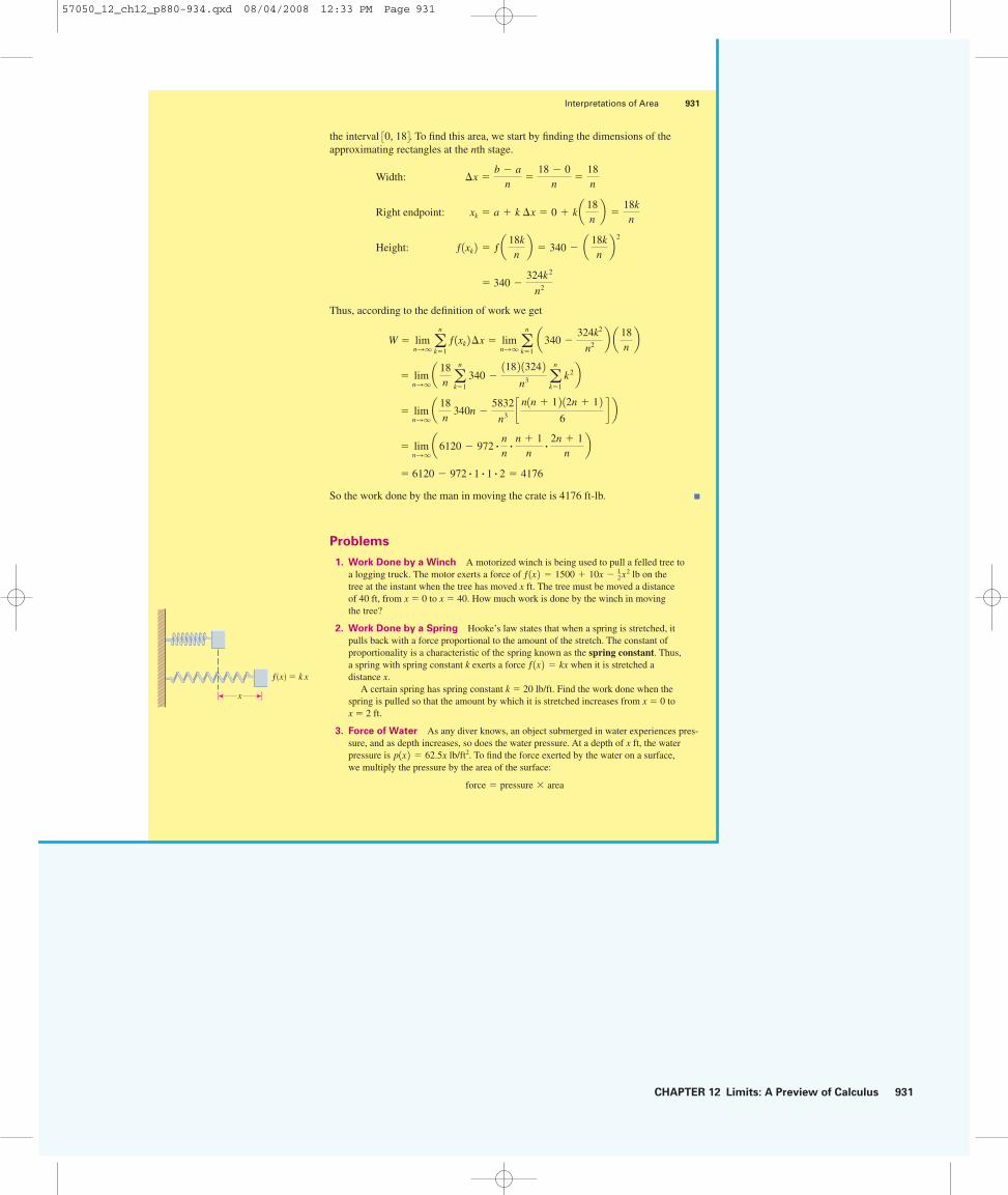
CHAPTER 12 Limits: A Preview of Calculus 931
the interval 30, 184. To find this area, we start by finding the dimensions of the approximating rectangles at the nth stage.
Width:
Right endpoint:
Height:
Thus, according to the definition of work we get
So the work done by the man in moving the crate is 4176 ft-lb. ■
Problems
1. Work Done by a Winch A motorized winch is being used to pull a felled tree to a logging truck. The motor exerts a force of lb on the tree at the instant when the tree has moved x ft. The tree must be moved a distance of 40 ft, from x � 0 to x � 40. How much work is done by the winch in moving the tree?
2. Work Done by a Spring Hooke’s law states that when a spring is stretched, it pulls back with a force proportional to the amount of the stretch. The constant of proportionality is a characteristic of the spring known as the spring constant. Thus,a spring with spring constant k exerts a force when it is stretched a distance x.
A certain spring has spring constant k � 20 lb/ft. Find the work done when the spring is pulled so that the amount by which it is stretched increases from x � 0 to x � 2 ft.
3. Force of Water As any diver knows, an object submerged in water experiences pres-sure, and as depth increases, so does the water pressure. At a depth of x ft, the waterpressure is lb/ft2. To find the force exerted by the water on a surface,we multiply the pressure by the area of the surface:
force � pressure � area
p1x 2 � 62.5x
f 1x 2 � kx
f 1x 2 � 1500 � 10x � 12x2
� 6120 � 972 # 1 # 1 # 2 � 4176
� limn�qa6120 � 972 # n
n# n � 1
n# 2n � 1
nb
� limn�qa 18
n 340n �
5832
n3 c n1n � 1 2 12n � 1 26
d b � lim
n�qa 18
n an
k�1340 �
118 2 1324 2n3 a
n
k�1k2 b
W � limn�qa
n
k�1f 1xk 2¢x � lim
n�qan
k�1a340 �
324k2
n2 b a 18nb
� 340 �324k2
n2
f 1xk 2 � f a 18knb � 340 � a 18k
nb 2
xk � a � k ¢x � 0 � k a 18nb �
18kn
¢x �b � a
n�
18 � 0n
�18n
Interpretations of Area 931
Ï=kx
x
57050_12_ch12_p880-934.qxd 08/04/2008 12:33 PM Page 931

932 CHAPTER 12 Limits: A Preview of Calculus
Suppose an aquarium that is 3 ft wide, 6 ft long, and 4 ft high is full of water. The bottom of the aquarium has area 3 � 6 � 18 ft2, and it experiences water pressure of
lb/ft2. Thus, the total force exerted by the water on the bottomis 250 � 18 � 4500 lb.
The water also exerts a force on the sides of the aquarium, but this is not as easy tocalculate because the pressure increases from top to bottom. To calculate the force onone of the 4 ft by 6 ft sides, we divide its area into n thin horizontal strips of width ¢x,as shown in the figure. The area of each strip is
If the bottom of the kth strip is at the depth xk, then it experiences water pressure of approximately lb/ft2—the thinner the strip, the more accurate the approximation. Thus, on each strip the water exerts a force of
(a) Explain why the total force exerted by the water on the 4 ft by 6 ft sides of the aquarium is
where ¢x � 4/n and xk � 4k/n.
(b) What area does the limit in part (a) represent?
(c) Evaluate the limit in part (a) to find the force exerted by the water on one of the 4 ftby 6 ft sides of the aquarium.
(d) Use the same technique to find the force exerted by the water on one of the 4 ft by 3 ft sides of the aquarium.
NOTE Engineers use the technique outlined in this problem to find the total force exerted on a dam by the water in the reservoir behind the dam.
4. Distance Traveled by a Car Since distance � speed � time, it is easy to see that a car moving, say, at 70 mi/h for 5 h will travel a distance of 350 mi. But what if the speed varies, as it usually does in practice?
(a) Suppose the speed of a moving object at time t is . Explain why the distancetraveled by the object between times t � a and t � b is the area under the graph of √ between t � a and t � b.
(b) The speed of a car t seconds after it starts moving is given by the functionft/s. Find the distance traveled by the car from t � 0 to
t � 5 s.
5. Heating Capacity If the outdoor temperature reaches a maximum of 90 �F one day and only 80 �F the next, then we would probably say that the first day was hotter than the second. Suppose, however, that on the first day the temperature was below 60 �F for most of the day, reaching the high only briefly, whereas on the second day the temperature stayed above 75 �F all the time. Now which day is the hotter one? To bettermeasure how hot a particular day is, scientists use the concept of heating degree-hour.If the temperature is a constant D degrees for t hours, then the “heating capacity”generated over this period is Dt heating degree-hours:
If the temperature is not constant, then the number of heating degree-hours equals the
heating degree-hours � temperature � time
√1t 2 � 6t � 0.1t3
√1t 2
limn�qa
n
k�1375xk ¢x
pressure � area � 62.5xk � 6 ¢x � 375xk ¢x lb
p1xk 2 � 62.5xk
length � width � 6 ¢x
p14 2 � 62.5 � 4 � 250
932 Focus on Modeling
0
xk
x(depth)
4 ft
6 ft3 ft
Îx
57050_12_ch12_p880-934.qxd 08/04/2008 12:33 PM Page 932
CHAPTER 12 Limits: A Preview of Calculus 933
area under the graph of the temperature function over the time period in question.
(a) On a particular day, the temperature (in �F) was modeled by the function, where t was measured in hours since midnight. How many
heating degree-hours were experienced on this day, from t � 0 to t � 24?
(b) What was the maximum temperature on the day described in part (a)?
(c) On another day, the temperature (in �F) was modeled by the function. How many heating degree-hours were experienced on
this day?
(d) What was the maximum temperature on the day described in part (c)?
(e) Which day was “hotter”?
E1t 2 � 50 � 5t � 14t2
D1t 2 � 61 � 65t � 1
25t2
Interpretations of Area 933
57050_12_ch12_p880-934.qxd 08/04/2008 12:33 PM Page 933

57050_12_ch12_p880-934.qxd 09/04/2008 03:35 PM Page 934