5044 ieee transactions on signal processing, vol. 58, no

5044 IEEE TRANSACTIONS ON SIGNAL PROCESSING, VOL. 58, NO. 10, OCTOBER 2010

Estimating Multiple Frequency-Hopping SignalParameters via Sparse Linear Regression

Daniele Angelosante, Member, IEEE, Georgios B. Giannakis, Fellow, IEEE, andNicholas D. Sidiropoulos, Fellow, IEEE

Abstract—Frequency hopping (FH) signals have well-docu-mented merits for commercial and military applications due totheir near-far resistance and robustness to jamming. EstimatingFH signal parameters (e.g., hopping instants, carriers, and am-plitudes) is an important and challenging task, but optimumestimation incurs an unrealistic computational burden. The spec-trogram has long been the starting non-parametric estimator in thiscontext, followed by line spectra refinements. The problem is thathop timing estimates derived from the spectrogram are coarse andunreliable, thus severely limiting performance. A novel approachis developed in this paper, based on sparse linear regression (SLR).Using a dense frequency grid, the problem is formulated as one ofunder-determined linear regression with a dual sparsity penalty,and its exact solution is obtained using the alternating directionmethod of multipliers (ADMoM). The SLR-based approach isfurther broadened to encompass polynomial-phase hopping (PPH)signals, encountered in chirp spread spectrum modulation. Sim-ulations demonstrate that the developed estimator outperformsspectrogram-based alternatives, especially with regard to hoptiming estimation, which is the crux of the problem.

Index Terms—Compressive sampling, frequency hopping sig-nals, sparse linear regression, spectrogram, spread spectrumsignals.

I. INTRODUCTION

F REQUENCY-HOPPING spread-spectrum signaling iswidely adopted in tactical communications due to its low

probability of detection and interception, agility, and robustnessto jamming [34]. Estimating and tracking the parameters ofmultiple superimposed FH signals are important tasks withapplications in both military and civilian domains: from in-terception of noncooperative communications, to collisionavoidance and cognitive radio. The problem is particularly

Manuscript received October 26, 2009; accepted June 01, 2010. Date of pub-lication June 10, 2010; date of current version September 15, 2010. The as-sociate editor coordinating the review of this manuscript and approving it forpublication was Prof. Sofia C. Olhede. The work in this paper was supportedby NSF Grants CCF 0830480 and CON 0824007, and also through collabora-tive participation in the Communications and Networks Consortium sponsoredby the U.S. Army Research Laboratory under the Collaborative Technology Al-liance Program, Cooperative Agreement DAAD19-01-2-0011. The U.S. Gov-ernment is authorized to reproduce and distribute reprints for Government pur-poses notwithstanding any copyright notation thereon. Part of the results in thispaper was presented at the International Conference on Acoustics, Speech andSignal Processing, Dallas, TX, April 2010.

D. Angelosante and G. B. Giannakis are with the Department of Electricaland Computer Engineering, University of Minnesota, Minneapolis, MN 55455USA (e-mail: [email protected]; [email protected]).

N. D. Sidiropoulos is with the Department of Electronic and Computer Engi-neering, Technical University of Crete, 73100, Chania, Crete, Greece (e-mail:[email protected]).

Digital Object Identifier 10.1109/TSP.2010.2052614

challenging when the hopping patterns of the constituent sig-nals are unknown, and, in addition to dwell frequency, hoptiming is randomized as well for added protection. Maximumlikelihood (ML) estimation is practically intractable in thiscontext, which motivates the pursuit of alternative low- tomoderate-complexity solutions.

Starting from coarse channelization techniques based on thespectrogram and related non-parametric time-frequency esti-mation tools, there is considerable literature on the subject ofFH signal parameter estimation and tracking. Non-parametricmethods based on the spectrogram are simple but suffer fromlimited resolution and require further refinements [1], [29].Time-frequency distribution techniques have been investigatedin [2] for acquisition of FH signals.

Parametric methods for FH signal estimation model the activefrequency as piecewise-constant and achieve improved estima-tion accuracy at the cost of higher complexity. The crux of theoverall problem is hop timing estimation: given the hop instants,what remains is essentially a sequence of harmonic retrievalproblems. When the hops are periodic, the timing problem re-duces to estimating the hopping period(s) and offset(s) [1], [2],[29]. Hop timing estimators for the more difficult case of ape-riodic hop timing have been developed based on dynamic pro-gramming (DP) [22], [23], and the expectation-maximization(EM) algorithm [24]. The algorithms in [22], [23] and [24] re-quire multiple receive antennas, and rely on the spectrogram forcoarse acquisition.

When only one FH signal is present, an effective particle fil-tering solution based on a stochastic dynamical system formu-lation has recently appeared in [36]. Different from [22], [23]and [24], the approach in [36] allows for sequential processing,and is robust to various sources of mismatch in the probabilisticmodel adopted. The limitation of [36] is that it does not gener-alize to multiple FH signals, due to the curse of dimensionality:the required number of particles grows fast with the dimension-ality of the state-space. The complexity of DP-based approaches[22], [23], on the other hand, increases rapidly also with thenumber of temporal samples—thus only short data records canbe processed.

While sparse linear regression (SLR) has been advocated in[10] and [16] for harmonic retrieval without carrier hopping, inthis paper a novel SLR-based technique is developed for mul-tiple FH signals. Relative to [10] and [16], here we also take ad-vantage of sparsity in terms of carrier hopping, which is effectedthrough a dual sparsity penalty. The developed estimator is alsogeneralized to handle polynomial-phase hopping (PPH) signalsthat emerge in chirp spread spectrum communications [6], [21],

1053-587X/$26.00 © 2010 IEEE

ANGELOSANTE et al.: ESTIMATING MULTIPLE FH SIGNAL PARAMETERS VIA SLR 5045

[28]. A pertinent sparsity-aware optimization problem is formu-lated and solved using the alternating direction method of multi-pliers (ADMoM). Simulations illustrate that the developed tech-nique is robust to model mismatch, and far outperforms spec-trogram-based methods, especially with regard to hop timingestimation.

Due to the non-convexity of the FH estimation problem, para-metric techniques based on the likelihood function (such as theEM algorithm) can be trapped in local minima if the initializa-tion is far from a global minimum. Due to its low complexityand high accuracy, the novel SLR-based estimator can be usedboth as a stand-alone FH signal estimation algorithm, and as anexcellent initialization for iterative refinement algorithms, suchas the one in [24].

Interestingly, the closely related problem of identifyingthe parameters of a piecewise-sinusoidal mixture model from(generalized) samples has been studied in [5] using a finite-rateof innovation (FRI) approach. SLR and FRI are different toolsdealing with similar problems; see also [9] for a tutorial on FRIand its relation with SLR and compressive sampling. Whileintroducing interesting identifiability conditions and algorithmsfor perfect reconstruction of the underlying continuous-timesignal, the approach in [5] is not directly applicable to thepresent context. The switching instants (“hops”) in [5] are con-tinuous variables, and the measurements are obtained throughanalog pre-filtering with a properly chosen kernel waveform,which may or may not be affordable. Since the hopping stepsare not instantaneous in practice [34], the present algorithm(as well as all existing alternatives for acquiring FH signals[22]–[24], [36]) do not attempt to localize the exact hoppinginstants, but rather aim to detect hops. Also, PPH signals arenot considered in [5]. On the other hand, numerical simulationssuggest that a suitable modification of the SLR estimator forthe noiseless case can perfectly recover the sampled FH signalsas well.

The rest of this paper is structured as follows. Section II con-tains preliminaries, and the problem statement. The novel SLRformulation is introduced in Section III, where sparsity tuningand extensions to PPH signals are also presented. An efficientsolution based on the ADMoM is developed in Section IV. Sim-ulations are presented in Section V, and conclusions are drawnin Section VI.

Notation: Column vectors (matrices) are denoted withlower-case (upper-case) boldface letters and sets with calli-graphic letters; stands for transposition, for con-jugate transposition, and for pseudoinverse;denotes the complex Gaussian probability density functionwith mean and variance denotes the Kroneckerproduct; and denote the real and imaginary part of

, respectively; is the -dimensional column vectorwith all zeros and is the -dimensional identity matrix,while denotes the matrix with all zeros. The(pseudo) -norm of is defined as the number of nonzeroelements of . The -, -, and -norms of aredefined, respectively, as

, and

.

II. PRELIMINARIES AND PROBLEM STATEMENT

Consider the noiseless signal , which at timeconsists of pure tones; that is

(1)

where is the th system-wise hopping instant1 [22],is the th system-wise dwell, and

are the complex amplitude andfrequency of the th tone in the th system-wise dwell, re-spectively. The number of tones, , can also vary with ,due to emitter (de)activation or bandwidth mismatch [24]. Theentire observation interval is . A noncooperativeasynchronous scenario is considered; hop timing is aperiodic,and independent across transmitters. Our approach is geared to-ward slow FH signals, and offsets due to frequency modulationcan be accommodated as well. The measured continuous-timewaveform is corrupted by additive circularly-symmetriccomplex white Gaussian noise , i.e.,

(2)

Let denote the total number of system-wise hops in ,and the period with which is sampledat the receiving end. The discrete-time FH signal can be writtenas [cf. (1)]

(3)

where, and . Corre-

spondingly, the discrete-time noisy observations are [cf. (2)]

(4)

where is white, and .Given , the objective is to estimate

, and . Since ML estimation of FHsignal parameters is practically intractable, non-parametric es-timators based on the spectrogram have been traditionally em-ployed. These are outlined briefly in the next subsection in orderto establish notation and context for the novel approach we willdevelop in Section III.

A. Spectrogram-Based Estimators

The spectrogram of is the squared modulus of theshort-term Fourier transform defined as

(5)

1The set of system-wise hopping instants is the union of all individual emitterhopping instants, splitting the time axis in system-wise dwells.


for , and. Specifically, one splits the observed data into

overlapping segments, windows with ,and computes the discrete Fourier transform (DFT) evaluatedat frequencies. Parameters , and the windowhighly affect the performance of spectrogram-based FH param-eter estimators. A large yields improved frequency resolu-tion, but poor temporal resolution which blurs hop timing. Small

blurs the frequency axis, and close-by hops become indis-tinguishable. This unyielding tradeoff is the major limitationof spectrogram-based estimation, and it also affects parametrictechniques which employ the spectrogram for coarse acquisi-tion. Two types of spectrogram-based techniques have been pro-posed in the literature for (aperiodic) hop timing estimation.

1) Entropy-based techniques [22]. The columns of the spec-trogram matrix formed with entries as in (5) are normal-ized to sum to unity, and the entropy of each column iscomputed. With denoting the sequence ofentropies, FH causes spectral spreading that translates tohigher entropy. This suggests obtaining the hopping in-stants by picking the peaks of ; and

2) Gradient techniques [24]. After setting to zero the entrieswhich are smaller than a predefined threshold

(typically equal to the sample mean of the spectrogram),the sum of the difference of consecutive columns isevaluated, i.e., ,for . The system-wise hoppinginstants can then be estimated by picking the peaks of .

These estimates are subsequently processed for further re-finement. Once hopping instants are acquired, the parameterswithin each dwell are estimated via harmonic retrieval tech-niques [22], [24].

The method developed in the sequel can be used as an effec-tive stand-alone solution that jointly recovers hop timing andthe remaining parameters of interest, namely , dwell fre-quencies, and amplitudes. Alternatively, the novel method canbe used to extract timing estimates, to be passed on to succes-sive stages (e.g., those described in [22] and [24]) for furtherrefinement.

III. ESTIMATION VIA SLR

Suppose that the true frequencies in (3) belong to aknown finite set with cardinality

. Note that this is not a limiting assumption for civilianapplications, provided that Doppler is negligible. In cases wherethis information is not available, the set can be a dense gridsuch that the separation between two consecutive frequenciesin is less than the desired resolution (in the same spirit of[10], [16] for harmonic retrieval). Clearly, as the preselected

increases the density of the grid increases, and so does thefrequency resolution—what in the sparse linear regression par-lance is referred to as super-resolution [16].

With , the received noisy samples can berewritten as

(6)

where , and. Observe that represents

the amplitude and phase of the th frequency bin attime . Since , a few of the coefficients

, representing the active frequencies at each time,are nonzero. Letting , and

, the model in

(3) and (4) can be expressed in vector-matrix form as

(7)

where , and .The FH signal parameters to estimate can be obtained from

, which obeys the linear regression model in (7). Matrixrepresents the time-localized

frequency content of the signal, and is related to the spectro-gram.

The key advantage of introducing the grid of candidate fre-quencies is that the nonlinear parameter estimation task athand is converted to a linear one [cf. (7)]. This is possible byincreasing the problem dimensionality through the selection of

. Note also that as the matrix is fat,the least-squares (LS) solution with minimum norm, namely

, does not yield an accurate estimate ofeven when the signal-to-noise ratio (SNR) is high. Improved

alternatives are possible however, if one capitalizes on the factthat the unknown vector exhibits the following two sparsityproperties.

1) Active carrier-domain sparsity. Only a few of the coeffi-cients are nonzero, which implies that in (7) issparse.

2) Differential time-domain sparsity (smoothness). Since FHis assumed slow, most of the time; hence,each row of is piecewise constant. This means thatadjacent row-wise differences are sparse.

Consider now the matrix

(8)

where , and the notation

represents the right cyclic shift of positions. Fromthe definition in (8), the th entry of contains thedifference ; hence, as mentioned earlier, is asparse vector.

Ideally, one would form a sparse and piecewise constant es-timate of by solving the following optimization problem:

(9)

The first term of the cost function in (9) takes into account theobserved signal while the positive scalars and control the


intrinsic sparsity and smoothness of the estimate, respectively.However, the problem in (9) is non-convex and NP-hard.

Motivated by recent advances in variable selection [33] andcompressive sampling [13], the -norm is relaxed with theconvex -norm. Hence, the advocated formulation becomes

(10)

Large effects sparsity, and large effects smoothness. Since, the second -norm

penalty in (10) captures the sum of total variation penalties.A couple of remarks are now in order.Remark 1. One motivation behind SLR-based harmonic re-

trieval in [10] and [16] is that non-uniform sampling can beaccommodated—a case of interest, e.g., in astronomy or whenobservations are missing. Parametric and subspace-based high-resolution algorithms (such as ESPRIT and MUSIC) can affordnon-uniform sampling only under suitable identifiability condi-tions (such as shift invariance); see e.g., [30]. Similar to [10],[16], the novel FH parameter estimator in (10) remains opera-tional even with non-uniformly sampled data, thanks to the grid-based formulation. In this case, ,where denotes the acquisition time of the th sample.

Remark 2. If , (10) is known as the least-absoluteshrinkage and selection operator (Lasso) [33]. With ,the cost in (10) is similar to the one utilized by the fused Lassoin [19].

The optimization problem in (10) is convex because the costcomprises the sum of an -norm term and an -norm term,both of which are convex by definition; hence, the cost in (10)can be minimized via interior point solvers, which are compu-tationally affordable for small-to-medium size problems [32].Since the non-differentiable part in (10) is not separable coordi-nate-wise, convergence to a global optimum of coordinate-de-scent solvers [35] cannot be invoked for large-size problems.An iterative algorithm to approximate the solution of the fusedLasso is developed in [19]. On the other hand, a low-complexityalgorithm to solve (10) exactly will be derived in Section IV.Before presenting this solution, it is of interest to explore usefulproperties of the estimator in (10) as a function of the scalarsand .

A. Guidelines for Choosing and

Selection of the regularization parameters affectscritically the performance of the estimator in (10). While under-regularizing may not be sufficient to retrieve the signal of in-terest, over-regularization can result in poor and biased esti-mates. Of course, if the number of tones present can be pro-vided a priori by other means, e.g., by inspecting the spectro-gram, can be tuned accordingly by trial and error. But ingeneral, analytical methods to automatically choose the “best”values of and are not available. In essence, selecting theregularization parameters is more a matter of engineering art,rather than systematic science.

In this subsection, heuristic but useful guidelines will be pro-vided to choose based on rigorously established lower

bounds of these parameters. To bound , we will rely on thefollowing result, which was derived in [25].

Proposition 1. If , then if and only if.

Proposition 1 asserts that if is greater than a thresholdspecified by the regression matrix and the observations, and

, then (10) yields estimates that are identically zero. Thisproperty of the Lasso has been exploited in [10] to select thepenalty parameter . In the present context of FH signal esti-mation, the implication is that must be chosen strictly lessthan in order to prevent the all-zero solution. Our extensivesimulations suggest that setting equal to a small percentageof , say 5%–10%, results in satisfactory estimates; see alsoSection V.

Turning our attention to bound the selection of , let de-note the lower triangular matrix with all nonzero entriesequal to one. Define , and partition the matrixproduct into and , sothat . Using these definitions, we have estab-lished the following property of the SLR estimator in (10); seeAppendix A for the proof.

Proposition 2. If , and has full column rank, thenwith , if and only

if .

If exceeds a threshold which is specified by the regres-sion matrix and the observations, and , Proposition 2implies that the estimates in (10) are constant in time; that is, allfrequency bins are hop-free. To avoid this trivial (non-FH) so-lution, the guideline provided by Proposition 2 is that mustbe chosen strictly less than . As with , the simulations ofSection V will demonstrate that setting to a small percentageof yields satisfactory estimation performance.

Remark 3. The scalars weighting the regularization termsalso affects the bias present in the estimators obtained as in (10).Specifically, note that biases towards zero, whichmay render the complex exponential amplitude estimates unre-liable. While the proposed back-off in selecting the regulariza-tion parameters relative to the bounds in Propositions 1–2 canlimit this bias, several strategies can be adopted to correct it. Asimple way for correcting the bias is to first acquire the hops (orhops plus frequencies) via (10), and then solve a line spectrum(correspondingly, amplitude) estimation problem for each dwellin-between the detected hops. A drawback of this per-dwell ap-proach is that it does not exploit the possible correlation presentacross adjacent dwells [cf. Section V-C].

Another approach to correct the bias in sparse regression isto retain only the support of (10) and re-estimate the amplitudesvia, e.g., LS. Notice that this approach is not directly appli-cable here because the number of non-zero entries of in (10)is generally in the order of , while the number of equa-tions in (7) is ; that is, the resultant linear regression modelis still under-determined. However, one can take advantage ofthe fact that the vector estimate is not only sparse but alsopiecewise constant. To this end, summing the columns ofcorresponding to the entries of that are equal, it is possible toreduce the number of unknowns.


An alternative approach to reducing the bias is through non-convex regularization using e.g., the smoothly clipped absolutedeviation (SCAD) scheme [18]. SCAD reduces bias withoutsuffering from the inherent limitations of per-dwell processing.Its limitation is that the cost is nonconvex, thus rendering exactminimization problematic due to the presence of local minima.A viable way for retaining the efficiency of convex optimizationwhile simultaneously limiting the bias due to the regularizingterm, is to resort to weighted norms [14], [37], [38]. Largerweights are given to terms that are most likely to be zero, whilesmaller weights are assigned to those that are most likely to benonzero. Given an initial solution , the weighted normis defined as , where isa decreasing function of its argument (see [14], [37], [38] forthree different weight functions). LS, ridge regression, or the(unweighted) estimator in (10) can be used for initialization.

B. Noiseless Case and Perfect Reconstruction

In this subsection, the SLR-estimator is tailored to the case ofnoiseless data. Consider the model

(11)

For this noise-free model, the idea is to replace the LS part of thecost in (10) with an exact constraint involving the linear systemof equations in (11). Specifically, the proposed modification of(10) is

(12)

Since is fat, the linear system admits an infinitenumber of solutions. The rationale behind (12) is to select thesolution that minimizes the cost . Theparameter is tuned to strike a desirable tradeoff between spar-sity and smoothness. Indeed, the larger the the smoother thesolution, and the smaller the the sparser the solution.

The question that arises at this point is whether coincideswith . Introducing an auxiliary variable, , theproblem in (12) can be rewritten as

(13)

Definingand

the optimization in (13) can be recast as a standard sparse signalreconstruction problem, namely

(14)

Sufficient conditions ensuring equivalence of (14) with the-norm based optimization for exact recovery are based either

on the restricted isometry property (RIP) or the incoherence

conditions on the columns of ; see [4], [11], [12] and referencestherein. Having shown that (12) reduces to (14) establishes thatany scheme available for checking the RIP or incoherence condi-tions applies here too. In addition, the simulations of Section Vindicate that if the parameter is chosen properly, the formula-tion in (12) can perfectly reconstruct the true .

It is also worth stressing that matrix (and thus ) in cer-tain applications is prescribed, and it is not up to the designer’schoice. For these applications, one focuses on the -norm basedsparse recovery and the aforementioned equivalence as well asthe RIP and incoherence conditions are not an issue.

Nonetheless, when the designer has the freedom to select , itis certainly interesting to know how the choice of affects thesesufficient conditions. With regards to checking their validity, it isalso pertinent to underscore that RIP analysis entails the nonzerosupport of the vector , as well as a “sufficiently small” con-stant . Hence, whether satisfies the RIP depends on the un-derlying and the chosen ; and this is NP-hard to check [12],[13]. Checking the incoherence conditions is feasible in poly-nomial time, but even when the columns of are “sufficientlyincoherent,” the implied RIP (bounds) may yield values forand , which may not be always practical [4].

Yet another major consideration constraining the choice ofin practice is the density of the grid points forming the entriesof . This density affects the attainable frequency resolution,which has to be balanced with the size of and the associatedcomplexity in solving the optimization problem (12).

C. Generalization to PPH Signals

Signals described by (3) and (6) are encountered in many en-gineering applications. However, certain modulation types in-duce both continuous and abrupt frequency changes that do notobey this model. The goal of this section is to broaden the scopeof the novel SLR-based FH estimation approach to polynomial-phase hopping (PPH) signals.

Polynomial-phase models are very important in radar signalprocessing, where relative velocity and acceleration are key pa-rameters of interest; e.g., see [3], [20] and references therein. Dueto inertia, however, model parameters change slowly in radar ap-plications. Instead of radar, the motivation for PPH comes fromchirp modulation, a digital communication technique originallyproposed during the 1960s. Various generalizations and applica-tions of chirp modulation have appeared since, including chirpspread spectrum multiplexing—see [6], [21], [28] and referencestherein. Instead of using a windowed carrier as the basic pulse,chirp modulation uses a windowed chirp, whose frequency is lin-early swept up or down to represent a logical 0 or 1. Multipleslopes (and offsets) can be used for -ary modulation, and/orto multiplex different users. Chirp modulation has a number ofdesirable properties relative to traditional FH, including robust-ness to Doppler and fading. In chirp modulation (multiplexing),abrupt changes of the PPH parameters occur at the boundary be-tween symbol periods (“dwells”).

The discrete-time model of a PPH signal can be written as

(15)


Observe that the model in (15) coincides with (3) when ,while for it includes also a linear-chirp hopping signal.For simplicity in exposition, the case is detailed next.

Suppose that the parameters and in

(15) belong to finite sets and

, respectively. Again, if this isnot the case, and represent dense grids that ap-proximate the true parameters and . If

this is the case, define

, and ,with . Upon properly defining , thediscrete-time signal in (15) can be written as

(16)

At the receiver, is corrupted by additive noise ,and observed as . Defining

, and lettingand denote the observation and noisevectors, the received vector becomes

(17)

where . Again,is sparse and piecewise constant. Letting

, and

(18)

the proposed SLR-based estimator for PPH signals is

(19)

Clearly, by simply replacing the regression matrix with ,the SLR estimator in (10) developed for FH signals carries overto the wider class of PPH signals.

IV. EFFICIENT IMPLEMENTATION VIA ADMOM

A low-complexity algorithm is developed in this section toobtain in (10). The crux of the advocated solver of the opti-mization problem in (10) is to show how the alternating direc-tion method of multipliers (ADMoM) [8, pp. 243–253] can beapplied to the problem at hand.

Consider re-writing the minimization in (10) with the use ofauxiliary variables and , as

(20)

Associating Lagrange multipliers with the equality con-straints, the quadratically augmented Lagrangian of the problemin (20) is

(21)

Selecting any positive number as well as arbitrary initialvectors , the ADMoM algorithm iteratesover the following steps:

(22)

(23)

(24)

(25)

With the auxiliary variables and the multipliers available fromthe st iteration, the wanted vector at iteration isobtained as in (22). Because in (21) is linear-quadratic in ,in Appendix B is shown that this convex minimization problemaccepts a closed-form solution, namely

(26)

Having found and with the multipliers fixed from thest iteration, the auxiliary variables at iteration

are subsequently obtained as in (23). After neglecting irrelevantterms, the pertinent minimization problem reduces to

(27)

Clearly, the cost in (27) can be minimized separately in and. Since the resulting minimizers w.r.t. and are found anal-

ogously, only the minimization over is detailed for brevity.

Noting that, the min-

imization in (27) over can be solved coordinate-wise; that is,for each coordinate , the problem to solve is

(28)


Albeit non-differentiable, the scalar convex cost in (28) can besolved in closed form. Specifically, we show in Appendix B thatthe solution of (28) is given by

(29)

which corresponds to the complex version of the soft shrinkageoperator in, e.g., [17]. Collecting the coordinate minimizers ina vector, the closed-form solution of (23) can be compactly ex-pressed using the vector shrinkage operator with entries as in(29), namely

(30)

(31)

Furthermore, note that the Lagrange multipliers are subse-quently updated as in (24) and (25), which are first-order, leastmean-square (LMS)-like iterations.

In a nutshell, the primal problem in (10) can be decoupled inthe minimization problems (22) and (23), which entail closed-form solutions per iteration plus simple Lagrange multiplier up-dates implemented as in (24) and (25). Apart from simplicity inimplementation, this iterative algorithm for SLR-based FH pa-rameter estimation is provably convergent to in (10), sincethe ADMoM is guaranteed to converge to a global minimizerfor convex functions [8, p. 253]. Summarizing, we have estab-lished the following.

Proposition 3. For any and , theiterates in (26), and in (30) and (31), as well as

and in (24) and (25), are all convergent. Specifically,converges to the solution of (10); that is, .

It is worth stressing at this point that the ADMoM solver ofthe SLR problem in (10) and the associated convergence resultin Proposition 3 are not confined to the FH/PPH signal estima-tion problem dealt with here. In fact, they carry over to all prob-lems that fused Lasso can be applied [19]. An extra attractivefeature of the ADMoM algorithm in (26)–(31) is that the ma-trix to be inverted in (26) remains fixed during the iterations;hence, the matrix inversion in (26) can be performed off-line.With obtained off-line, the com-putational complexity per iteration is dominated by the multi-plication in (26), that is . Furthermore, since the ma-trix is very sparse [cf. (7) and (8)],solving (26) for large and can be facilitated via computa-tionally efficient solvers of sparse linear systems of equations,such as the conjugate gradient algorithm [7, p. 130]. In addition,the ADMoM can afford a convergent distributed implementa-tion which is also robust to noisy links [27]—a useful attributewhen estimation is to be performed using wireless sensor net-works, where observations are spatially distributed.

Fig. 1. Two hopping complex exponentials. (a) True time-frequency pattern;(b) spectrogram; (c) sparse linear regression estimates; (d) entropy of the (nor-malized) spectrogram estimates, � ; (e) sum of the difference of consecutivecolumns of the spectrogram, �; (f) � � �� .

A. Noiseless Case

Similar to (10), the estimator in (12) admits an efficient imple-mentation via the ADMoM. Indeed, mimicking the steps used tosolve the minimization problem in (10), the following holds true.

Proposition 4. For any theiterates

(32)

(33)

(34)

(35)

(36)

(37)

converge to the solution of (12); that is, .

V. SIMULATIONS

In this section, the developed algorithms are tested in severalscenarios.

A. Frequency Hopping and Hop Timing Estimation

The signal of interest in (3) and (6) consists of two hop-ping tones, while the grid of carriers is chosen to be

with , and . The first FH tone isgenerated to be active on the 10th carrier in the interval [0, 9],and then hops to the 20th carrier during the interval [10, 47]. Thesecond hopping tone occupies the 25th carrier in the interval [0,29], and the 5th carrier in the interval [30, 47]. The two FH sig-nals are in-phase and have equal amplitude.

The true time-frequency pattern of the signal of interest is de-picted in Fig. 1(a). (Here and in what follows the squared mod-ulus of the entries is plotted.) The spectrogram obtained with


Fig. 2. Two hopping complex exponentials. Probability of incorrect detectionversus SNR �� .

, and using a rectangular windowis shown in Fig. 1(b) at10 dB. In Fig. 1(c), the modulus of the estimate in (10) rear-ranged in matrix form, i.e., , is depicted for

and , with as in Proposition 1(correspondingly 2). Here and in what follows these scaling pa-rameters are used unless specified otherwise. ADMoMupdates in (22)–(25) are terminated either after a fixed numberof (here ) iterations, or, by using the following stopping cri-terion: . Observe thatis a far better estimate of the true time-frequency pattern thanthe spectrogram.

Fig. 1(d) and (e) depicts, respectively, the entropy sequence[22], and the gradient sequence [24] versus time.

Notice that the peaks of these statistics provide estimates ofthe system-wise hopping instants. In Fig. 1(f), the statistic

for isplotted. Clearly, represents a better statistic thanand to estimate the hopping instants.

Performance of the spectrogram- and SLR-based hop timingestimators is next assessed via Monte Carlo simulations. Thesignal of interest is the one in Fig. 1(a) and, for simplicity, thenumber of system-wise hops is assumed known. Thehop timing estimates are obtained by picking the peaks of

, and . To pick the peaks of those statistics, thefollowing steps are repeated times: i) The maximum valueof the statistic is found; ii) its index is stored; and iii) the valueof this entry and the adjacent entries are set to zero. Correctacquisition (CA) corresponds to having each of the estimatesof the hopping instants less than samples away from theassociated true hopping instants. Fig. 2 depicts the probabilityof incorrect acquisition versus SNR (aver-aged over noise realizations) for the two spectrogram-basedestimators, and the novel estimator in (10) with and

. Observe that the entropy-based technique outperformsthe gradient-based one, and the SLR estimator achieves the bestoverall performance.

Next, the tested signal of interest comprises FH tones:the two of Fig. 1(a) plus a third one that occupies the 15th car-rier in the interval [0, 19], and then hops to the 30th carrier inthe interval [20, 47]. With the parameters used in Fig. 1, the re-sulting signal together with the spectrogram, the SLR estimatesand the decision statistics are depicted in Fig. 3. Fig. 4 shows the

Fig. 3. Three hopping complex exponentials. (a) True time-frequency pattern;(b) spectrogram; (c) sparse linear regression estimates; (d) entropy of the (nor-malized) spectrogram estimates, � ; (e) Sum of the difference of consecutivecolumns of the spectrogram, �; (f) � � �� .

Fig. 4. Three hopping complex exponentials. Probability of incorrect detectionversus SNR versus SNR �� .

probability of incorrect acquisition versus SNR. Observe thatthe performance of the entropy-based estimator degrades whilethe SLR estimator achieves satisfactory performance.

So far, the true signal comprised a fixed number of complexexponentials hopping only once. Next, a case is tested where thenumber of complex exponentials varies across dwells and morehops occur. The first complex exponential occupies the 10th car-rier over the interval [0,9], then hops to the 20th carrier over [10,34], and to the 30th carrier over [35, 47]. The second complexexponential occupies the 15th carrier over [0,19] and then it dis-appears, while the third complex exponential occupies the 25thcarrier over the interval [0, 29], and the 5th carrier over [30, 47].With the parameters identical to those used in Fig. 1, the resultingsignal along with the spectrogram, the SLR estimates, and thedecision statistics are depicted in Fig. 5. The selection strategiesadvocated in Section III-A are seen effective also in this case ofmultiple hops and a varying number of tones per dwell.

B. Robustness to Sources of Model Mismatch

In Section V-A the signal of interest was a superposition ofideal complex exponentials that hopped within a known fre-quency grid. In this subsection, the estimator in (10) is tested inthe presence of various sources of mismatch between the modelin (3), (4), and (6) and the signal of interest. First, a carrier mis-match is considered.


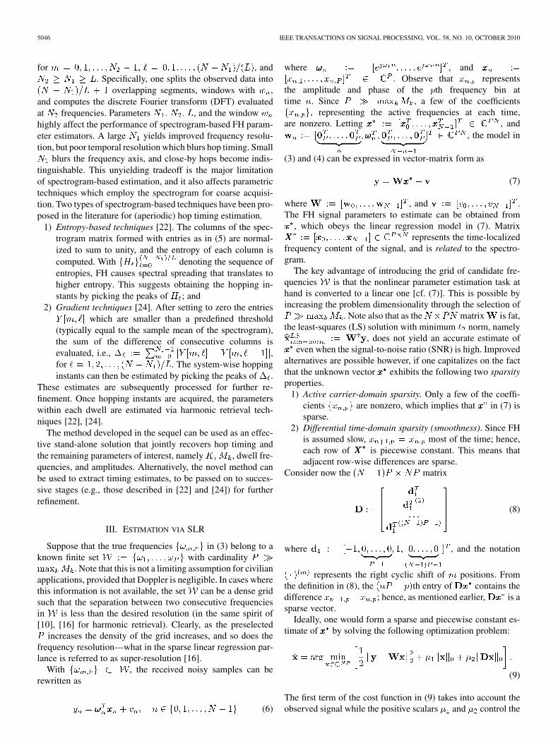
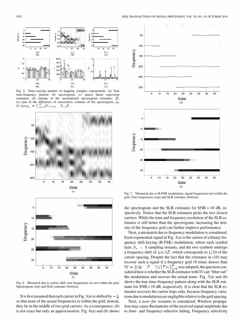
Fig. 5. Time-varying number of hopping complex exponentials. (a) Truetime-frequency pattern; (b) spectrogram; (c) sparse linear regressionestimates; (d) entropy of the (normalized) spectrogram estimates, � ;(e) sum of the difference of consecutive columns of the spectrogram, �;(f) � � �� .

Fig. 6. Mismatch due to carrier shift: true frequencies are not within the grid.Spectrogram (top) and SLR estimates (bottom).

It is first assumed that each carrier in Fig. 3(a) is shifted byso that none of the actual frequencies is within the grid; instead,they lie in the middle of two grid carriers. As a consequence, (6)is not exact but only an approximation. Fig. 6(a) and (b) shows

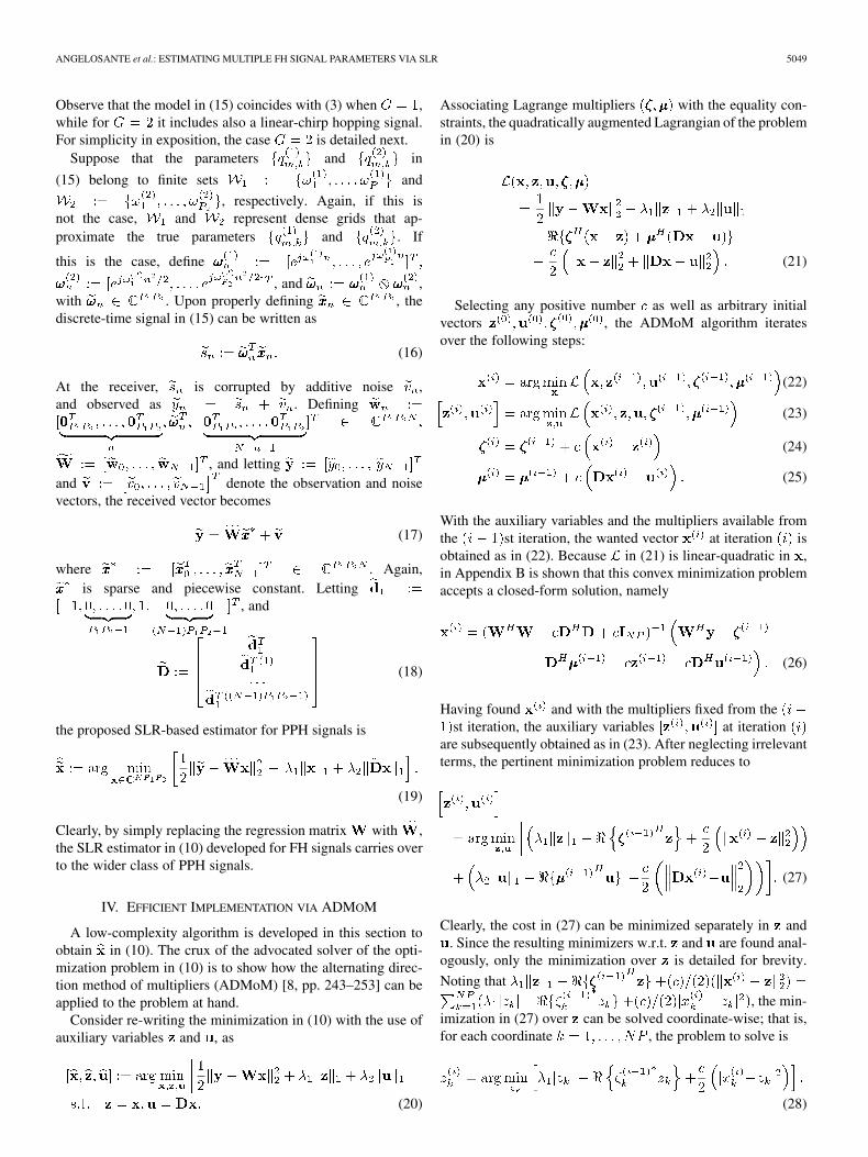
Fig. 7. Mismatch due to B-FSK modulation: signal frequencies not within thegrid. True frequencies (top) and SLR estimates (bottom).

the spectrogram and the SLR estimates for SNR = 10 dB, re-spectively. Notice that the SLR estimator picks the two closestcarriers. While the time and frequency resolution of the SLR es-timator is still better than the spectrogram, increasing the den-sity of the frequency grid can further improve performance.

Next, a mismatch due to frequency modulation is considered.Each exponential signal in Fig. 3(a) is the carrier of a binary fre-quency shift keying (B-FSK) modulation, where each symbollasts sampling instants, and the two symbols undergoa frequency shift of , which corresponds to of thecarrier spacing. Despite the fact that the estimator in (10) mayrecover such a signal if a frequency grid 10 times denser than

was adopted, the question con-sidered here is whether the SLR estimator with can “filter out”the modulation and recover the actual tones. Fig. 7(a) and (b)shows the true time-frequency pattern along with the SLR esti-mate for SNR = 10 dB, respectively. It is clear that the SLR es-timator recovers the carrier hops only, because frequency varia-tions due to modulation are negligible relative to the grid spacing.

Next, a near–far scenario is considered. Wireless propaga-tion may cause fluctuations of the received signal amplitude dueto time- and frequency-selective fading. Frequency selectivity


Fig. 8. Mismatch due to fading. The complex exponential amplitudes are timevarying. True signal (top) and SLR estimates (bottom).

means that different tones are subject to different attenuationand phase shift; time selectivity means that the attenuation andphase shift of a given tone vary with time. If this is the case, exactreconstruction of the signals of interest is impossible, becausethe number of unknowns is much larger than the number of ob-servations. In many cases, however, fading only induces rela-tively small fluctuations around a nominal amplitude. Indeed,Fig. 8(a) and (b) depicts the signal of interest affected by time-varying fading, and its SLR estimate for SNR = 10 dB. Thenonzero time-varying amplitude coefficients in (6) are generatedas a first-order Gauss–Markov process, i.e.,

with , and .Interestingly, the developed estimator is able to recover the truetime-localized frequency pattern, and “average out” small am-plitude variations due to fading.

C. Noiseless Case

In this subsection, the noiseless reconstruction algorithm of(12) is tested. The signal of interest is the one in Fig. 3(a). Fig. 9shows the squared error (SE), , versus the iterationindex of the algorithm in Proposition 4 for , andvarious values of . Surprisingly, if properly tuned, the SLRestimator in (12) can perfectly recover the signal .

Fig. 9. Evolution of the squared-error in the noise-free case.

Fig. 10. Evolution of the squared-error in the noise-free case (dwell-wise iden-tifiability is not met).

Once hop timing is acquired, one can solve a set of harmonicretrieval problems on a per-dwell basis to obtain refined fre-quency and complex amplitude estimates [22], [24]. This kind ofprocessing is clearly suboptimum, since it does not take into ac-count observations of adjacent dwells—which contain informa-tion about the frequency content in the dwell of interest. Param-eter identifiability for the per-dwell harmonic retrieval problemgoes back to Caratheodory [15]; see also [31]. Assuming dis-tinct dwell frequencies, it turns out that identifiability of thisnonlinear problem boils down to counting equations-versus-un-knowns: for complex exponentials within the dwell, oneneeds at least observations (length of the dwell).2

Next, a case similar to Fig. 3(a) is considered except that thefirst signal hops to the 20th carrier at time 18, so that only onesample is taken during the second dwell. In this case, per-dwellprocessing fails to recover the signal within the second dwelleven with perfect knowledge of the hop timing. Fig. 10 showsthe SE versus the iteration index (i) of the algorithm in Proposi-tion 4 with . Observe that the SLR estimator is capable

2There are three real unknowns per complex exponential, and two real equa-tions per complex measurement.


of recovering the signal of interest perfectly. This is possible be-cause the estimator in (12) exploits the frequency smoothnessalong adjacent dwells. Clearly, this does not constitute an iden-tifiability claim; what it does demonstrate, however, is that theSLR estimator is capable of perfect recovery in situations whereper-dwell processing unequivocally fails.

D. PPH Signal Estimation

In this subsection, the generalization of the SLR es-timator to PPH signals is tested. A mixture of FH andlinear chirp hopping signals is considered. Specifically,the chosen parameters are:

and. The signal of interest is a super-

position of FH signals in , and hopping chirp signals in .The particular choice of is not instrumental in any wayother than allowing for easy visualization: it guarantees that theinstantaneous frequency of the chirp signals at every samplepoint belongs to .

The signal of interest was generated as the superposition oftwo signals. The first occupies the 7th carrier in the interval[0,24], and then hops to the 12th carrier in the interval [25, 47].The second signal occupies the 15th carrier in the interval [0,14], and then turns into a linearly decreasing chirp starting fromthe 18th carrier in the interval [15,31], and finally to a linearlyincreasing chirp starting from the 5th carrier in the interval [32,47]. Fig. 11(a) and (b) shows the true time-frequency patternalong with the SLR estimate for SNR = 10 dB, ,and . It is worth noting that since theassumption of Proposition 2 is not met. As expected, the SLRestimator correctly recovers the frequency content of the signalof interest.

VI. CONCLUSION

A novel technique was introduced to estimate FH signal pa-rameters based on sparse linear regression. Earlier approachesrely upon the spectrogram of the received signal, at least forcoarse acquisition. The estimation task was formulated here asan under-determined linear regression problem with a dual spar-sity penalty. Its exact solution was obtained using the ADMoM.Guidelines were provided to select the regularization parame-ters, and the estimation approach was generalized to PPH sig-nals. Simulations demonstrated that the novel technique out-performs spectrogram-based estimators by a significant margin,especially with regard to hop-timing estimation. A modifica-tion of the novel estimator in the noiseless case revealed thatthe SLR estimator can perfectly recover the signal of interest,even when per-dwell identifiability fails—thus holding greaterpromise than per-dwell processing approaches. The ADMoM-based algorithm developed here for FH/PPH signal estimationcan be ported to other problems, such as applications of fusedLasso [19]. Interesting extensions of this work can be pursuedin slowly time-varying line spectrum estimation.3

3The views and conclusions contained in this document are those of the au-thors and should not be interpreted as representing the official policies, eitherexpressed or implied, of the Army Research Laboratory or the U. S. Govern-ment.

Fig. 11. Estimation of polynomial-phase hopping signals. True signal (top) andSLR estimates (bottom).

APPENDIX

A. Proof of Proposition 2

With , the problem in (10) simplifies to

(38)

Recall that , and let

(39)

Defining , it holds that

(40)

and

(41)


Hence, an equivalent form of (38) is

(42)

where

(43)

The necessary and sufficient first-order optimality condition forto be the (unconstrained) minimum of , is that

the subgradient of evaluated at contains thezero vector [26, p. 92], i.e.,

(44)

Defining

(45)

the subgradient of evaluated at can be ex-pressed as

(46)

where the th entry of is

(47)

with such that .From (46) and (47), (44) translates to the following condi-

tions:c1) , for ; and,

c2) for

.The constant (i.e., hop-free) solution corresponds to havingand . Thus, c1) implies that

(48)

which is uniquely satisfied by since has fullcolumn rank. Hence, and if and onlyif c2) is satisfied, which corresponds to for

, or equivalently, .

B. Proof of Proposition 3

It suffices to show that the problems in (22) and (23) admit theclosed-form solution in (26) and (30)–(31), respectively. Afterskipping constant terms, (22) can be written as

(49)

Upon equating the gradient of the convex differentiable cost tozero, the expression in (26) is readily obtained.

In Section IV we have showed that (23) can be separated inscalar problems of the form in (28). Next, we show that (28) ad-mits the closed-form solution in (29). Because the cost in (28) isconvex but non-differentiable, the necessary and sufficient con-dition for to attain its minimum is [26, p. 92]

(50)

Substituting with the expression in (29), it is easy to verifythat the conditions in (50) are satisfied. This completes the proofof the proposition.

REFERENCES

[1] L. Aydin and A. Polydoros, “Hop-timing estimation for FH signalsusing a coarsely channelized receiver,” IEEE Trans. Commun., vol. 44,no. 4, pp. 516–526, Apr. 1996.

[2] S. Barbarossa and A. Scaglione, “Parameter estimation of spread spec-trum frequency-hopping signals using time-frequency distributions,”Proc. Signal Processing Advances in Wireless Commun., pp. 213–216,Apr. 1997.

[3] S. Barbarossa, A. Scaglione, and G. B. Giannakis, “Product high-orderambiguity function for multicomponent polynomial phase signal mod-eling,” IEEE Trans. Signal Process., vol. 46, no. 3, pp. 691–708, Mar.1998.

[4] Z. Ben-Haim, Y. C. Eldar, and M. Elad, “Coherence-based perfor-mance guarantees for estimating a sparse vector under random noise,”IEEE Trans. Signal Process., 10.1109/TSP.2010.2052460, to be pub-lished.

[5] J. Berent, P. L. Dragotti, and T. Blu, “Sampling piecewise sinusoidalsignals with finite rate of innovation methods,” IEEE Trans. SignalProcess., vol. 58, no. 2, pp. 613–625, Feb. 2010.

[6] A. Berni and W. Gregg, “On the utility of chirp modulation for digitalsignaling,” IEEE Trans. Commun., vol. 21, no. 6, pp. 748–751, Jun.1973.

[7] D. Bertsekas, Non Linear Programming, 2nd ed. Singapore: AthenaScientific, 2003.

[8] D. P. Bertsekas and J. N. Tsitsiklis, Parallel and Distributed Com-putation: Numerical Methods, 2nd ed. Singapore: Athena Scientific,1999.

[9] T. Blu, P.-L. Dragotti, M. Vetterli, P. Marziliano, and L. Coulot,“Sparse sampling of signal innovations: Theory, algorithms, andperformance bounds,” IEEE Signal Process. Mag., vol. 25, pp. 31–40,Mar. 2008.

[10] S. Bourguignon, H. Carfantan, and J. Idier, “A sparsity-based methodfor the estimation of spectral lines from irregularly sampled data,” IEEEJ. Sel. Topics Signal Process., vol. 1, no. 4, pp. 575–585, Dec. 2007.

[11] T. T. Cai, G. Xu, and J. Zhang, “On recovery of sparse signals via �

minimization,” IEEE Trans. Inf. Theory, vol. 55, no. 7, pp. 3388–3397,Jul. 2009.

[12] E. J. Candès and T. Tao, “Decoding by linear programming,” IEEETrans. Inf. Theory, vol. 51, no. 12, pp. 4203–4215, Dec. 2005.

[13] E. Candès and M. B. Wakin, “An introduction to compressive sam-pling,” IEEE Signal Process. Mag., vol. 25, pp. 21–30, Mar. 2008.

[14] E. Candès, M. Wakin, and S. Boyd, “Enhancing sparsity by reweighted� minimization,” J. Fourier Anal. Appl., vol. 14, pp. 877–905, 2007.

[15] C. Carathéodory and L. Fejér, “Uber den Zusammenghang der Ex-temen von harmonischen Funktionen mit ihren Koeffizienten und uberden Picard-Landauschen Satz,” Rendiconti del Circolo Matematico diPalermo, vol. 32, pp. 218–239, 1911.

[16] S. S. Chen and D. L. Donoho, “Application of basis pursuit in spec-trum estimation,” in Proc. Int. Conf. Acoust., Speech, Signal Process.,Seattle, WA, May 1998, vol. 3, pp. 1865–1868.

[17] M. Elad, B. Matalon, J. Shtok, and M. Zibulevsky, “A wide-angle viewat iterated shrinkage algorithms,” presented at the SPIE (Wavelet XII),San Diego, CA, Aug. 2007.

[18] J. Fan and R. Li, “Variable selection via nonconcave penalized like-lihood and its oracle properties,” J. Amer. Stat. Assoc., vol. 96, pp.1348–1360, 2001.

[19] J. Friedman, T. Hastie, H. Höfling, and R. Tibshirani, “Pathwise coor-dinate optimization,” Ann. Appl. Stat., vol. 1, pp. 302–332, Dec. 2007.


[20] F. Gini and G. B. Giannakis, “Hybrid FM-polynomial phase signalmodeling: Parameter estimation and Cramer–Rao bounds,” IEEETrans. Signal Process., vol. 47, no. 2, pp. 363–377, Feb. 1999.

[21] S. Hengstler, D. P. Kasilingam, and A. H. Costa, “A novel chirp mod-ulation spread spectrum technique for multiple access,” in Proc. 7thIEEE Int. Symp. Spread Spectrum Techniques Applications, 2002, vol.1, pp. 73–77.

[22] X. Liu, N. D. Sidiropoulos, and A. Swami, “Blind high-resolution lo-calization and tracking of multiple frequency hopped signals,” IEEETrans. Signal Process., vol. 50, no. 4, pp. 889–901, Apr. 2002.

[23] X. Liu, N. D. Sidiropoulos, and A. Swami, “Joint hop timing and fre-quency estimation for collision resolution in frequency-hopped net-works,” IEEE Trans. Wireless Commun., vol. 4, no. 6, pp. 3063–3074,Nov. 2005.

[24] X. Liu, J. Li, and X. Ma, “An EM algorithm for blind hop timing es-timation of multiple FH signals using an array system with bandwidthmismatch,” IEEE Trans. Veh. Technol., vol. 56, no. 5, pp. 2545–2554,Sep. 2007.

[25] M. R. Osborne, B. Presnell, and B. A. Turlach, “On the LASSO and itsdual,” J. Comput. Graph. Stat., vol. 9, pp. 319–337, Jun. 2000.

[26] A. Ruszczynski, Nonlinear Optimization. Princeton, NJ: PrincetonUniv. Press, 2006.

[27] I. D. Schizas, A. Ribeiro, and G. B. Giannakis, “Consensus in Ad HocWSNs with noisy links—Part I: Distributed estimation of deterministicsignals,” IEEE Trans. Signal Process., vol. 56, no. 1, pp. 350–364, Jan.2008.

[28] H. Shen, S. Machineni, C. Gupta, and A. Papandreou-Suppappola,“Time-varying multichirp rate modulation for multiple access systems,”IEEE Signal Process. Lett., vol. 11, no. 5, pp. 497–500, May 2004.

[29] M. K. Simon, U. Cheng, L. Aydin, A. Polydoros, and B. K. Levitt, “Hoptiming estimation for noncoherent frequency-hopped M-FSK interceptreceivers,” IEEE Trans. Commun., vol. 43, no. 2/3/4, pp. 1144–1154,Feb./Mar./Apr. 1995.

[30] P. Stoica and R. Moses, Spectral Analysis of Signals. EnglewoodCliffs, NJ: Prentice-Hall, 2005.

[31] P. Stoica and T. Soderstom, “Parameter identifiability problems insignal processing,” Proc. Inst. Electr. Eng. F—Radar Sonar Navig.,vol. 141, pp. 133–136, 1994.

[32] J. Sturm, “Using Sedumi 1.02, a matlab toolbox for optimization oversymmetric cones,” Optim. Methods Softw., vol. 11, no. 12, pp. 625–653,1999.

[33] R. Tibshirani, “Regression shrinkage and selection via the Lasso,” J.Roy. Stat. Soc. Ser. B, vol. 58, no. 1, pp. 267–288, 1996.

[34] D. J. Torrieri, “Mobile frequency-hopping CDMA systems,” IEEETrans. Commun., vol. 48, no. 8, pp. 1318–1327, Aug. 2000.

[35] P. Tseng, “Convergence of block coordinate descent method fornon-differentiable minimization,” J. Optim. Theory Appl., vol. 109,pp. 475–494, Jun. 2001.

[36] A. Valyrakis, E. E. Tsakonas, N. D. Sidiropoulos, and A. Swami, “Sto-chastic modelling and particle filtering algorithms for tracking a fre-quency-hopped signal,” IEEE Trans. Signal Process., vol. 57, no. 8,pp. 3108–3118, Aug. 2009.

[37] H. Zou, “The adaptive Lasso and its oracle properties,” J. Amer. Stat.Assoc., vol. 101, no. 476, pp. 1418–1429, 2006.

[38] H. Zou and R. Li, “One-step sparse estimates in nonconcave penalizedlikelihood models,” Ann. Stat., vol. 36, no. 4, pp. 1509–1533, 2008.

Daniele Angelosante (M’09) was born in Frosinone,Italy, on June 1, 1981. He received the B.Sc., LaureaMagistrale, and Ph.D. degrees in telecommunicationengineering from the University of Cassino, Italy, in2003, 2005, and 2009, respectively, and the M.Sc.degree in electrical engineering with specialization insignal and information processing for communicationfrom the University of Aalborg, Denmark, in 2005.

From April to June 2007, he worked at the Univer-sity Pompeu Fabra, Spain. In 2008, he was a visitingscholar at the University of Minnesota, Minneapolis.

He is currently a Postdoctoral Associate with the Department of Electrical andComputer Engineering of the University of Minnesota. His research interests liein the areas of statistical signal processing, with emphasis on wireless commu-nications, tracking and compressed sensing.

Georgios B. Giannakis (F’97) received the Diplomadegree in electrical engineering from the NationalTechnical University of Athens, Greece, in 1981and the M.Sc. degree in electrical engineering, theM.Sc. degree in mathematics, and the Ph.D. degreein electrical engineering from the University ofSouthern California (USC) in 1983, 1986, and 1986,respectively.

Since 1999, he has been a Professor with the Uni-versity of Minnesota, where he now holds an ADCChair in Wireless Telecommunications in the Elec-

tric and Computer Engineering Department and serves as Director of the Dig-ital Technology Center. His general interests span the areas of communications,networking and statistical signal processing subjects on which he has publishedmore than 300 journal papers, 500 conference papers, two edited books, andtwo research monographs. Current research focuses on compressive sensing,cognitive radios, network coding, cross-layer designs, mobile ad hoc networks,wireless sensor, and social networks.

Dr. Giannakis is the (co-)inventor of 20 patents issued and the (co)recipient ofseven paper awards from the IEEE Signal Processing (SP) and CommunicationsSocieties, including the G. Marconi Prize Paper Award in Wireless Communi-cations. He also received Technical Achievement Awards from the SP Society(2000), from EURASIP (2005), a Young Faculty Teaching Award, and the G.W. Taylor Award for Distinguished Research from the University of Minnesota.He is a Fellow of EURASIP, and has served the IEEE in a number of posts, in-cluding that of Distinguished Lecturer for the IEEE SP Society.

Nicholas D. Sidiropoulos (F’09) received theDiploma degree from the Aristotelian University ofThessaloniki, Greece, and M.Sc. and Ph.D. degreesfrom the University of Maryland at College Park(UMCP), in 1988, 1990, and 1992, respectively, allin electrical engineering.

He has been a Postdoctoral Fellow (1994–1995)and Research Scientist (1996–1997) at the Institutefor Systems Research, UMCP, and has held positionsas Assistant Professor, Department of ElectricalEngineering, University of Virginia-Charlottesville

(1997–1999), and Associate Professor, Department of Electrical and ComputerEngineering, University of Minnesota—Minneapolis (2000–2002). Since2002, he has been a Professor in the Department of Electronic and ComputerEngineering at the Technical University of Crete, Chania-Crete, Greece, andAdjunct Professor at the University of Minnesota. His current research interestsare primarily in signal processing for communications, convex approximationof NP-hard problems, cross-layer resource allocation for wireless networks,and multiway analysis.

Prof. Sidiropoulos received the U.S. NSF CAREER Award in 1998 and theIEEE Signal Processing Society (SPS) Best Paper Award in 2001 and in 2007.He has served as a Distinguished Lecturer of the IEEE SPS (2008–2009), andas Chair (2007–2008) of the Signal Processing for Communications and Net-working Technical Committee of the IEEE SPS. He has also served as AssociateEditor for the IEEE TRANSACTIONS ON SIGNAL PROCESSING (2000–2006) andthe IEEE SIGNAL PROCESSING LETTERS (2000–2002), and currently serves onthe Editorial Board of the IEEE Signal Processing Magazine.

5044 ieee transactions on signal processing, vol. 58, no

Documents