Oscar Nierstrasz

5. Introduction to the Lambda Calculus

Roadmap

> What is Computability? — Church’s Thesis> Lambda Calculus — operational semantics> The Church-Rosser Property> Modelling basic programming constructs

References

> Paul Hudak, “Conception, Evolution, and Application of Functional Programming Languages,” ACM Computing Surveys 21/3, Sept. 1989, pp 359-411.

> Kenneth C. Louden, Programming Languages: Principles and Practice, PWS Publishing (Boston), 1993.

> H.P. Barendregt, The Lambda Calculus — Its Syntax and Semantics, North-Holland, 1984, Revised edition.

3

Roadmap

> What is Computability? — Church’s Thesis> Lambda Calculus — operational semantics> The Church-Rosser Property> Modelling basic programming constructs

What is Computable?

Computation is usually modelled as a mapping from inputs to outputs, carried out by a formal “machine,” or program, which processes its input in a sequence of steps.

An “effectively computable” function is one that can be computed in a finite amount of time using finite resources.

………………………

input

yes

nooutput

Effectively computable

function

5

Church’s Thesis

Effectively computable functions [from positive integers to positive integers] are just those definable in the lambda calculus.

Or, equivalently:

It is not possible to build a machine that is more powerful than a Turing machine.

Church’s thesis cannot be proven because “effectively computable” is an intuitive notion, not a mathematical one. It can only be refuted by giving a counter-example — a machine that can solve a problem not computable by a Turing machine.

So far, all models of effectively computable functions have shown to be equivalent to Turing machines (or the lambda calculus).

6

Uncomputability

A problem that cannot be solved by any Turing machine in finite time (or any equivalent formalism) is called uncomputable.

Assuming Church’s thesis is true, an uncomputable problem cannot be solved by any real computer.

The Halting Problem:Given an arbitrary Turing machine and its input tape, will the machine eventually halt?

The Halting Problem is provably uncomputable — which means that it cannot be solved in practice.

7

What is a Function? (I)

Extensional view:

A (total) function f: A → B is a subset of A × B (i.e., a relation) such that:

1. for each a ∈ A, there exists some (a,b) ∈ f(i.e., f(a) is defined), and

2. if (a,b1) ∈ f and (a, b2) ∈ f, then b1 = b2 (i.e., f(a) is unique)

8

The extensional view is the database view: a function is a particular set of mappings from arguments to values.

What is a Function? (II)

Intensional view:

A function f: A → B is an abstraction λx.e, where x is a variable name, and e is an expression, such that when a value a ∈ A is substituted for x in e, then this expression (i.e., f(a)) evaluates to some (unique) value b ∈ B.

9

The intensional view is the programmatic view: a function is a specification of how to transform the input argument to an output value.

NB: uniqueness does not come for free. The latter view is closer to that of programming languages, since infinite relations can only be represented intensionally.

Roadmap

> What is Computability? — Church’s Thesis> Lambda Calculus — operational semantics> The Church-Rosser Property> Modelling basic programming constructs

What is the Lambda Calculus?

The Lambda Calculus was invented by Alonzo Church [1932] as a mathematical formalism for expressing computation by functions.

Syntax:e ::= x a variable

| λ x . e an abstraction (function)| e1 e2 a (function) application

Examples:λ x . x — is a function taking an argument x, and returning xf x — is a function f applied to an argument x

NB: same as f(x) !

11

We have seen lambda abstractions before in Haskell with a very similar syntax: \ x -> x+1

is the anonymous Haskell function that adds 1 to its argument x. Function application in Haskell also has the same syntax as in the lambda calculus: Prelude> (\x ->x+1) 2

3

Parsing Lambda Expressions

Lambda extends as far as possible to the rightλ f.x y ≡ λ f.(x y)

Application is left-associativex y z ≡ (x y) z

Multiple lambdas may be suppressed λ f g.x ≡ λ f . λ g.x

12

What is the Lambda Calculus? ...

(Operational) Semantics:

The lambda calculus can be viewed as the simplest possible pure functional programming language.

α conversion (renaming):

λ x . e ↔ λ y . [ y/x ] e where y is not free in e

β reduction (application):

(λ x . e1) e2→ [ e2/x ] e1 avoiding name

capture

η reduction: λ x . e x → e if x is not free in e

13

The α conversion rule simply states that “variable names don't matter”. If you define a function with an argument x, you can change the name of x to y, as long as you do it consistently (change every x to y) and avoid name clashes (there must not be another [free] y in the same scope). The β reduction rule shows how to evaluate function application: just (syntactically) replace the formal parameter of the function body by the argument everywhere, taking care to avoid name clashes. Finally, the η reduction rule can be seen as a renaming optimization: if the body of a function just applies another function f to its argument, then we can replace that whole function by f. Note that the α rule only rewrites an expression but does not simplify it. That is why it is called a “conversion” and not a “reduction”.

Beta Reduction

Beta reduction is the computational engine of the lambda calculus:

Define: I ≡ λ x . x

Now consider:

I I = (λ x . x) (λ x . x ) → [λ x . x / x] x β reduction= λ x . x substitution= I

14

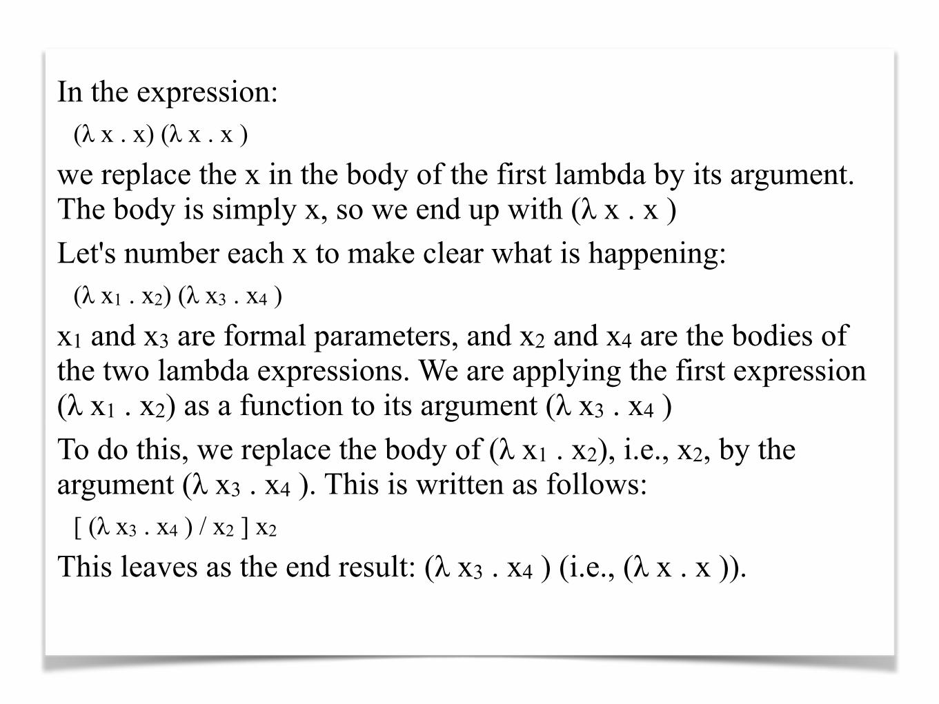
In the expression: (λ x . x) (λ x . x )

we replace the x in the body of the first lambda by its argument. The body is simply x, so we end up with (λ x . x ) Let's number each x to make clear what is happening:

(λ x1 . x2) (λ x3 . x4 )

x1 and x3 are formal parameters, and x2 and x4 are the bodies of the two lambda expressions. We are applying the first expression (λ x1 . x2) as a function to its argument (λ x3 . x4 ) To do this, we replace the body of (λ x1 . x2), i.e., x2, by the argument (λ x3 . x4 ). This is written as follows:

[ (λ x3 . x4 ) / x2 ] x2

This leaves as the end result: (λ x3 . x4 ) (i.e., (λ x . x )).

Lambda expressions in Haskell

We can implement many lambda expressions directly in Haskell:

Prelude> let i = \x -> xPrelude> i 55Prelude> i i 55

15

How is i i 5 parsed?

Lambdas are anonymous functions

A lambda abstraction is just an anonymous function.

Consider the Haskell function:

The value of compose is the anonymous lambda abstraction:λ f g x . f (g x)

NB: This is the same as:λ f . λ g . λ x . f (g x)

compose f g x = f(g(x))

16

Prelude> let compose = \f g x -> f(g x)

Prelude> compose (\x->x+1) (\x->x*2) 5

11

Free and Bound Variables

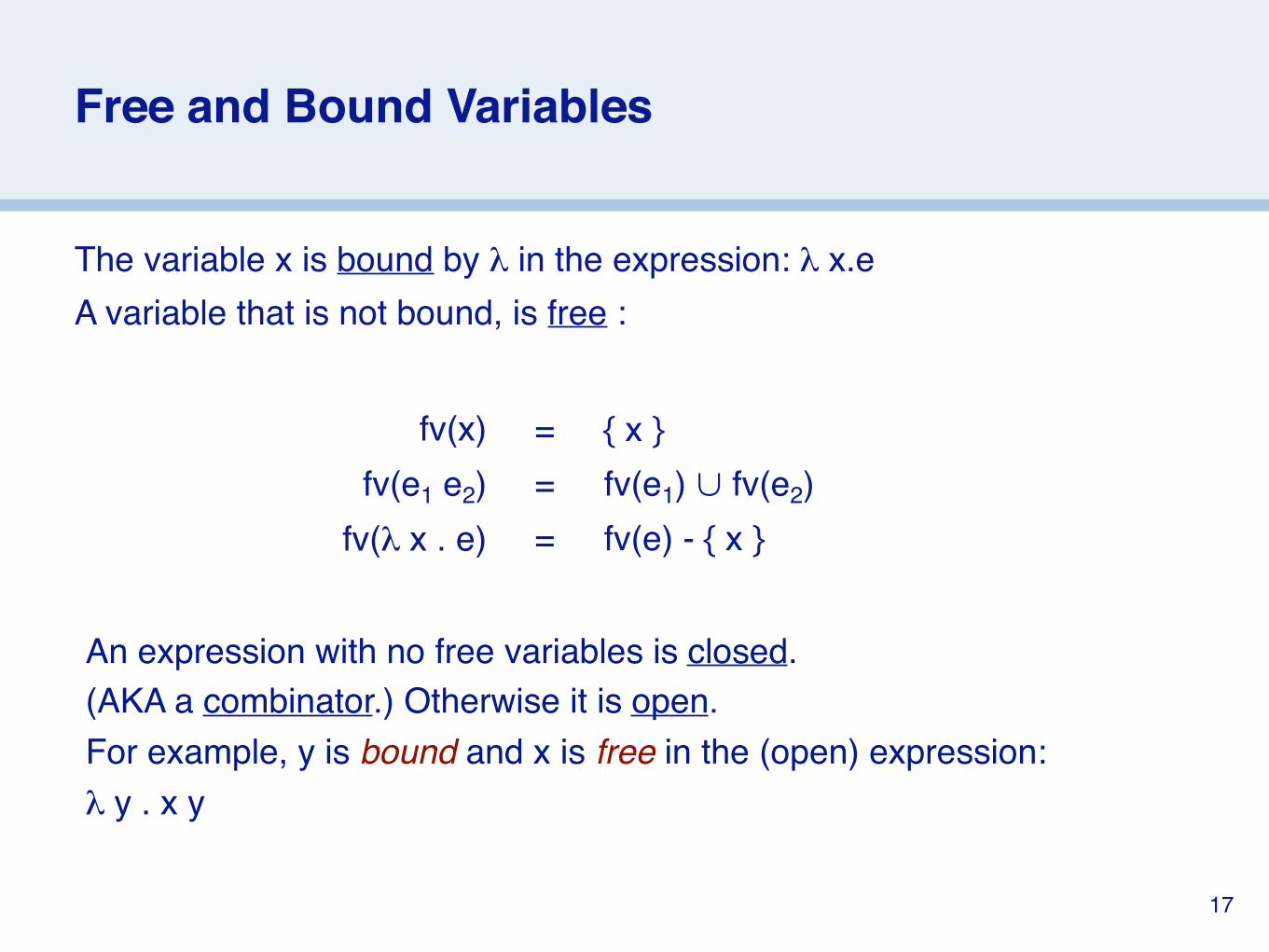
The variable x is bound by λ in the expression: λ x.eA variable that is not bound, is free :

An expression with no free variables is closed.(AKA a combinator.) Otherwise it is open.For example, y is bound and x is free in the (open) expression:λ y . x y

fv(x) = { x }fv(e1 e2) = fv(e1) ∪ fv(e2)

fv(λ x . e) = fv(e) - { x }

17

You can also think of bound variables as being defined. The expression λ x.e

defines the variable x within the body e, just like: int plus(int x, int y) { ... }

defines the variables x and y within the body of the Java method plus. A variable that is not defined in some outer scope by some lambda is “free”, or simply undefined. Closed expressions have no “undefined” variables. In statically typed programming languages, all procedures and programs are normally closed.

A Few Examples

1. (λx.x) y2. (λx.f x)3. x y4. (λx.x) (λx.x)5. (λx.x y) z6. (λx y.x) t f7. (λx y z.z x y) a b (λx y.x)8. (λf g.f g) (λx.x) (λx.x) z9. (λx y.x y) y10.(λx y.x y) (λx.x) (λx.x)11. (λx y.x y) ((λx.x) (λx.x))

18

Which variables are free? Which are bound?

“Hello World” in the Lambda Calculus

hello world

✎ Is this expression open? Closed?

19

Roadmap

> What is Computability? — Church’s Thesis> Lambda Calculus — operational semantics> The Church-Rosser Property> Modelling basic programming constructs

Why macro expansion is wrong

Syntactic substitution will not work:

(λ x y . x y ) y → [ y / x] (λ y . x y) β reduction≠ (λ y . y y ) incorrect substitution!

Since y is already bound in (λ y . x y), we cannot directly substitute y for x.

21

Substitution

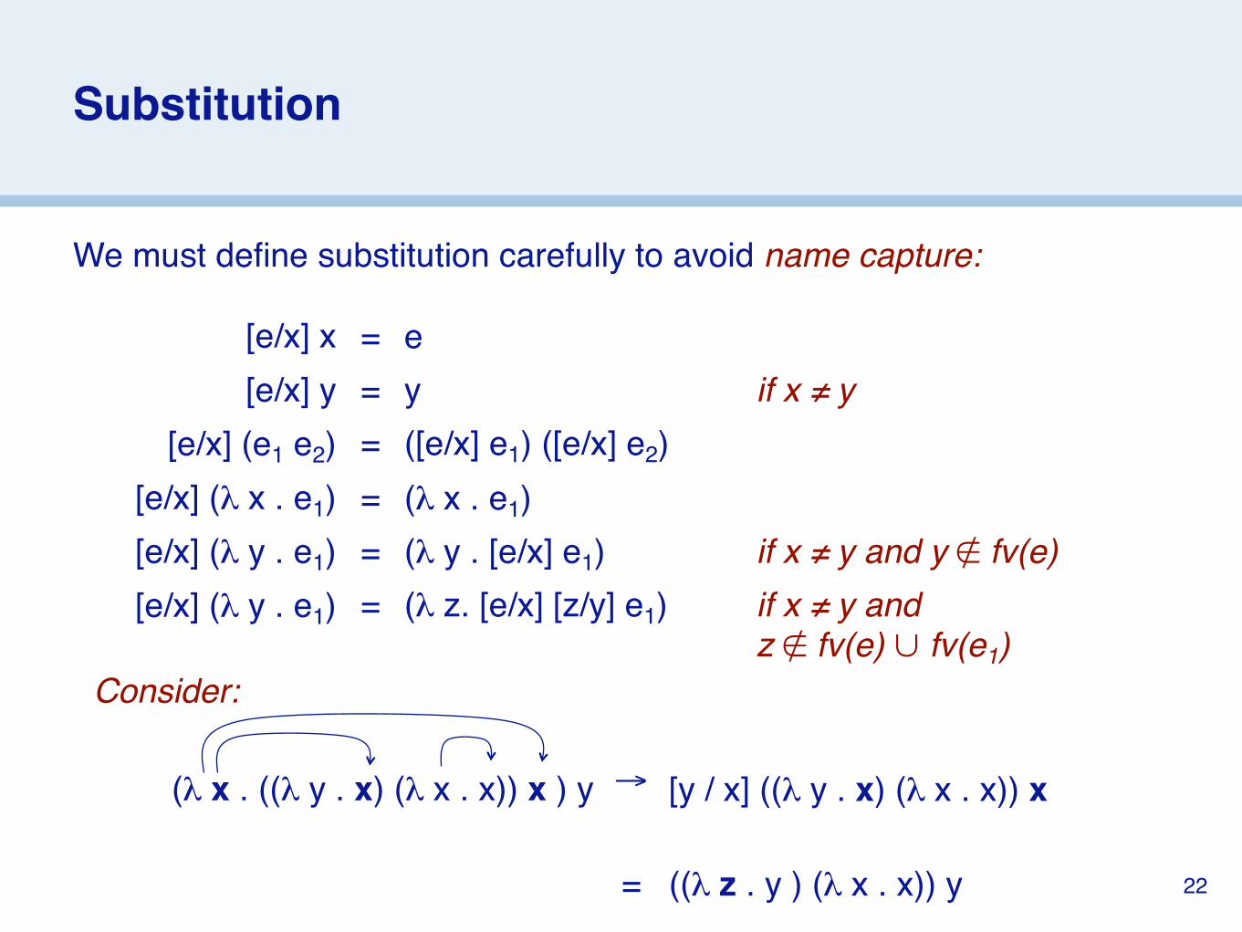
We must define substitution carefully to avoid name capture:

[e/x] x = e[e/x] y = y if x ≠ y

[e/x] (e1 e2) = ([e/x] e1) ([e/x] e2)[e/x] (λ x . e1) = (λ x . e1)[e/x] (λ y . e1) = (λ y . [e/x] e1) if x ≠ y and y ∉ fv(e)[e/x] (λ y . e1) = (λ z. [e/x] [z/y] e1) if x ≠ y and

z ∉ fv(e) ∪ fv(e1)

(λ x . ((λ y . x) (λ x . x)) x ) y → [y / x] ((λ y . x) (λ x . x)) x

= ((λ z . y ) (λ x . x)) y

Consider:

22

Of these six cases, only the last one is tricky. If the expression e (i.e., the argument to our function (λ y . e1)) contains a variable name y that conflicts with the formal parameter y of our function, then we must first rename y to a fresh name z in that function. After renaming y to z, there is no longer any conflict with the name y in our argument e, and we can proceed safely with the substitution.

Alpha Conversion

Alpha conversions allow us to rename bound variables.A bound name x in the lambda abstraction (λ x.e) may be substituted by any other name y, as long as there are no free occurrences of y in e:

Consider:(λ x y . x y ) y → (λ x z . x z) y α conversion

→ [ y / x] (λ z . x z) β reduction→ (λ z . y z)= y η reduction

23

Eta Reduction

Eta reductions allow one to remove “redundant lambdas”.Suppose that f is a closed expression (i.e., there are no free variables in f).

Then:(λ x . f x ) y → f y β reduction

So, (λ x . f x ) behaves the same as f !

Eta reduction says, whenever x does not occur free in f, we can rewrite (λ x . f x ) as f.

24

αβη

(λ x y . x y) (λ x . x y) (λ a b . a b) NB: left assoc.→ (λ x z . x z) (λ x . x y) (λ a b . a b) α conversion→ (λ z . (λ x . x y) z) (λ a b . a b) β reduction→ (λ x . x y) (λ a b . a b) β reduction→ (λ a b . a b) y β reduction→ (λ b . y b) β reduction→ y η reduction

25

Normal Forms

A lambda expression is in normal form if it can no longer be reduced by beta or eta reduction rules.Not all lambda expressions have normal forms!Ω = (λ x . x x) (λ x . x x)

→ [ (λ x . x x) / x ] ( x x )= (λ x . x x) (λ x . x x) β reduction→ (λ x . x x) (λ x . x x) β reduction→ (λ x . x x) (λ x . x x) β reduction→ ...

Reduction of a lambda expression to a normal form is analogous to a Turing machine halting or a program terminating.

26

A Few Examples

1. (λx.x) y2. (λx.f x)3. x y4. (λx.x) (λx.x)5. (λx.x y) z6. (λx y.x) t f7. (λx y z.z x y) a b (λx y.x)8. (λf g.f g) (λx.x) (λx.x) z9. (λx y.x y) y10.(λx y.x y) (λx.x) (λx.x)11. (λx y.x y) ((λx.x) (λx.x))

27

Are these in normal form?Can they be reduced?If so, how?

Evaluation Order

Most programming languages are strict, that is, all expressions passed to a function call are evaluated before control is passed to the function.Most modern functional languages, on the other hand, use lazy evaluation, that is, expressions are only evaluated when they are needed.

Consider:

Applicative-order reduction:

Normal-order reduction:

sqr n = n * n

sqr (2+5) ➪ sqr 7 ➪ 7*7 ➪ 49

sqr (2+5) ➪ (2+5) * (2+5) ➪ 7 * (2+5) ➪ 7 * 7 ➪ 49

28

The Church-Rosser Property

“If an expression can be evaluated at all, it can be evaluated by consistently using normal-order evaluation. If an expression can be evaluated in several different orders (mixing normal-order and applicative order reduction), then all of these evaluation orders yield the same result.”

So, evaluation order “does not matter” in the lambda calculus.

29

Roadmap

> What is Computability? — Church’s Thesis> Lambda Calculus — operational semantics> The Church-Rosser Property> Modelling basic programming constructs

Non-termination

However, applicative order reduction may not terminate, even if a normal form exists!

Compare to the Haskell expression:

(λ x . y) ( (λ x . x x) (λ x . x x) )Applicative order reduction Normal order reduction

→ (λ x . y) ( (λ x . x x) (λ x . x x) ) → y

→ (λ x . y) ( (λ x . x x) (λ x . x x) )

…

(\x -> \y -> x) 1 (5/0) ➪ 1

31

Currying

Since a lambda abstraction only binds a single variable, functions with multiple parameters must be modelled as Curried higher-order functions.

As we have seen, to improve readability, multiple lambdas are suppressed, so:

λ x y . x = λ x . λ y . xλ b x y . b x y = λ b . λ x . λ y . ( b x ) y

32

Don’t forget that functions written this way are still Curried, so arguments can be bound one at a time! In Haskell: Prelude> let f = (\ x y -> x) 1

Prelude> f 2

1

Representing Booleans

Many programming concepts can be directly expressed in the lambda calculus. Let us define:

True ≡ λ x y . xFalse ≡ λ x y . y

not ≡ λ b . b False Trueif b then x else y ≡ λ b x y . b x y

then:not True = (λ b . b False True ) (λ x y . x )

→ (λ x y . x ) False True→ False

if True then x else y = (λ b x y . b x y ) (λ x y . x) x y→ (λ x y . x) x y→ x 33

This is the “standard encoding” of Booleans as lambdas (other encodings are possible). A Boolean makes a choice between two values, a “true” one and a “false” one. True returns the first argument and False returns the second. Negation just reverses the logic, by passing False and True as arguments to the boolean: not True will return False and not False will return True.

Representing Tuples

Although tuples are not supported by the lambda calculus, they can easily be modelled as higher-order functions that “wrap” pairs of values.n-tuples can be modelled by composing pairs ...

Define: pair ≡ (λ x y z . z x y)first ≡ (λ p . p True )

second ≡ (λ p . p False )

then: (1, 2) = pair 1 2→ (λ z . z 1 2)

first (pair 1 2) → (pair 1 2) True→ True 1 2→ 1 34

The function pair takes three arguments. The first two arguments are the x and y values of the pair. Since pair is a Curried function, passing in x and y returns a function (i.e., a pair) that will take a third argument, z. The body of the pair will pass x and y to z, which can then bind x and y and do what it likes with them. As examples, consider the functions first and second. Each takes a pair p as argument and and passes it a boolean as the final argument z. These booleans respectively return x or y, i.e., the first or second value in the pair.

How would you define a lambda expression sum that takes a pair p as argument and returns the sum of the x and y values it contains?

Tuples as functions

In Haskell:

t = \x -> \y -> xf = \x -> \y -> ypair = \x -> \y -> \z -> z x y first = \p -> p tsecond = \p -> p f

Prelude> first (pair 1 2)1Prelude> first (second (pair 1 (pair 2 3)))2

35

What you should know!

✎ Is it possible to write a Pascal compiler that will generate code just for programs that terminate?

✎ What are the alpha, beta and eta conversion rules?✎ What is name capture? How does the lambda calculus

avoid it?✎ What is a normal form? How does one reach it?✎ What are normal and applicative order evaluation? ✎ Why is normal order evaluation called lazy?✎ How can Booleans and tuples be represented in the

lambda calculus?

Can you answer these questions?

✎ How can name capture occur in a programming language?

✎ What happens if you try to program Ω in Haskell? Why?✎ What do you get when you try to evaluate (pred 0)? What

does this mean?✎ How would you model numbers in the lambda calculus?

Fractions?

http://creativecommons.org/licenses/by-sa/4.0/

Attribution-ShareAlike 4.0 International (CC BY-SA 4.0)

You are free to:Share — copy and redistribute the material in any medium or formatAdapt — remix, transform, and build upon the material for any purpose, even commercially.

The licensor cannot revoke these freedoms as long as you follow the license terms.

Under the following terms:

Attribution — You must give appropriate credit, provide a link to the license, and indicate if changes were made. You may do so in any reasonable manner, but not in any way that suggests the licensor endorses you or your use.

ShareAlike — If you remix, transform, or build upon the material, you must distribute your contributions under the same license as the original.

No additional restrictions — You may not apply legal terms or technological measures that legally restrict others from doing anything the license permits.