5. finite element analysis of bellows -...

Ph. D. thesis on “Study of Design Aspects of Expansion Joints with Metallic Bellows and their Performance Evaluation” 139

5. Finite Element Analysis of Bellows

5.1 Introduction:

Traditional design process and stress analysis techniques are very specific for

each individual case based on fundamental principles. It can only be

satisfactorily applied to a range of conventional component shapes and

specific loading conditions using sound theories. Also this design process

needs continuous improvement till the product becomes matured and proven

successful by customers. After that the product becomes standardized. This

methodology is followed by majority industries for their products.

But in case of customized products, every individual product has unique

design features. Specific geometric parameters are altered in order to achieve

desirable function from the product. Hence, traditional design technique is not

much useful because of very frequent changes in the design calculations.

Expansion joints are such customized products, which needs to be treated

individually for varieties of applications. Every time design procedure is carried

out carefully and minor modifications are also required. During traditional

design process many ambiguities remains in the mind of designers because of

varieties of application areas of expansion joints. Thus, designers normally use

higher safety factors in order to minimize risk. This leads to over design

components by specifying either unnecessarily bulky cross sections or high

quality materials. Inevitably the cost of the product is adversely affected. Finite

Element Analysis (FEA) provides a better solution for design and stress

analysis in the virtual environment.

Finite Element Analysis (FEA) is a computer-based numerical technique for

calculating the strength and behavior of engineering structural components. It

can be used to calculate deflection, stress, vibration, buckling behavior and

many other phenomena. It can be used to analyze either small or large scale

deflection under loading or applied displacement. It can analyze elastic

deformation, as well as plastic deformation. Finite element analysis makes it

possible to evaluate in detail the complex structures, in a computer, during the


planning of the structure. The demonstration of adequate strength of the

structure and the possibility of improving the design during planning can justify

the need of this analysis work.

The first issue to understand in FEA is that it is fundamentally an

approximation. The underlying mathematical model may be an approximation

of physical system. The finite element itself approximates what happens in its

interior with the help of interpolating formulas.

In the finite element analysis, first step is modeling. Using any special CAD

software, model can be generated using the construction and editing features

of the software. In finite element method the structure is broken down into

many small simple blocks called elements. The material properties and the

governing relationships are considered over these elements. The behavior of

an individual element can be described with a relatively simple set of

equations. Just as the set of elements would be jointed together to build the

whole structure, the equations describing the behavior of the individual

elements are also joined into an extremely large set of equations that describe

the behavior of whole structure.

The computer can solve large set of simultaneous equations. From the

solutions, the computer extracts the behavior of the individual elements. From

this, it can get the stress and deflection of all parts of a structure. The stresses

will be compared to permissible values of stress for the materials to be used,

to see if the structures are strong enough.

Interpretation of the results requires knowing what is an acceptable

approximation, development of a complete list of what should be evaluated;

appreciation of the need of margin of safety, and comprehension of what

remains unknown after an analysis.

There are many softwares available for finite element analysis, which can be

utilized for the engineering applications. They are ANSYS, Pro/Engineer,

CATIA, NASTRAN, Hyper Works, I-DEAS etc.

5.2 Overview of FEA Procedure:

1. Modeling of the component


A model is required to be generated for the component which is to be

analyzed. Designer has to choose proper type of element for the analysis.

Actually the kind of component behavior is required to be considered at this

stage. The model can be either one dimensional, two dimensional or three

dimensional. One dimensional model can be generated by using 2 D spar

element; two dimensional models can be generated by key points or directly

generating two dimensional shapes like rectangle, circle, etc. Here union,

intersection and subtraction of area kind of commands are very useful. In case

of three dimensional modeling two dimensional shape can be extruded to third

direction, or revolve command is useful. Every designer can have own idea for

generating model. Many times component is consist of many small parts,

hence all parts are required to be modeled, than assembly function is required.

Here type of fit can also be selected as per requirements. Pro/Engineer

software is facilitating this kind of features. While earlier ANSYS software does

not provide assembly feature. This feature is added in workbench module. All

softwares are having their distinct features as well as limitations. User has to

make proper choice for applications.

2. Descritization of the continuum:

The continuum is the physical body, structure, or solid being analyzed.

Descritization may be simply described as the process in which the given body

is subdivided into an equivalent system of finite elements. Elements are

nothing but a small portion of the continuum which represents the whole

continuum that is being analyzed. The finite elements may be triangles, groups

of triangles or quadrilaterals for a two dimensional continuum. For three

dimensional analysis, the finite elements may be tetrahedral, rectangular

prisms or hexahedral.

In some cases the extent of the continuum to be modeled may not be clearly

defined. Only a significant portion of such a continuum needs to be considered

and descritized. Indeed, practical limitations require that on should include only

the significant portion of any large continuum in the finite element analysis.

3. Selection of the displacement models


The assumed displacement functions or models represent only approximately

the actual or exact distribution of the displacements. A displacement function is

commonly assumed to be a polynomial and practical considerations limit the

number of terms that can be retained in the polynomial. The simplest

displacement model that is commonly employed is a linear polynomial.

Obviously, it is generally not possible to select a displacement function that

can represent exactly the actual variation of displacement in the element.

Hence, the basic approximation of the finite element method is introduced at

this stage.

There are interrelated factors which influence the selection of a displacement

model. Usually, since a polynomial is chosen, only the degree of the

polynomial is open to decision. The particular displacement magnitudes that

describe the model must also be selected. These are usually the

displacements of the nodal points.

4. Derivation of the finite element stiffness matrix:

The stiffness matrix consists of the coefficients of the equilibrium equations

derived from the material and geometric properties of an element and obtained

by use of the principle of minimum potential energy. The stiffness relates the

displacements at the nodal points (the nodal displacement) to the applied

forces at the nodal points (the nodal forces). The distributed forces applied to

the structure are converted into equivalent concentrated forces at the nodes.

The equilibrium relation between the stiffness matrix [k], nodal force vector {Q},

and nodal displacement vector {q} is expresses as a set of simultaneous

algebraic equations,

[k] {q} = {Q} (5.1)

The elements of the stiffness matrix are the influence coefficients. A stiffness

of a structure is an influence coefficient that gives the force at one point on a

structure associated with a unit displacement of the same or a different point.

The stiffness matrix for an element depends upon (1) the displacement model,

(2) the geometry of the element, and (3) the local material properties. For an

elastic isotropic body, a pair of parameters such as the young’s modulus E and

the Poisson’s ratio define the local material properties. Since material


properties are assigned to a particular finite element, it is possible to account

for non-homogeneity by assigning different material properties to different finite

elements in the assemblage.

5. Assembly of the algebraic equations for the overall descritized continuum.

This process includes the assembly of the overall or global stiffness matrix for

the entire body from the individual element stiffness matrices, and the overall

global force or load vector from the element nodal force vectors. The most

common assembly technique is known as the direct stiffness method. In

general, the basis for an assembly method is that the nodal interconnections

require the displacements at a node to be the same for all elements adjacent

to that node. The overall equilibrium relations between the total stiffness matrix

[K], the total load vector {R}, and the nodal displacement vector for the entire

body {r} will again be expresses as a set of simultaneous equations.

[K] {r} = {R} (5.2)

These equations can not be solved until the geometric boundary conditions are

taken into account by appropriate modification of the equations. A geometric

boundary condition arises from the fact that displacements may be prescribed

at the boundaries or edges of the body or structure.

6. Solutions for the unknown displacements

The algebraic equations assembled in above step are solved for the unknown

displacements. For liner equilibrium problems, this is a straightforward

application of matrix algebra techniques. For non-linear problems, the desired

solutions are obtained by a sequence of steps, each step involving the

modification of the stiffness matrix and/or load vector.

7. Computation of the element strains and stresses from the nodal displacement

In certain cases the magnitudes of the primary unknowns, that is the nodal

displacements, will be all that are required for an engineering solution,. More

often, other quantities derived from the primary unknowns, such as strains

and/or stresses, must be computed.


The stresses and strains are proportional to the derivatives of the

displacements and in the domain of each element meaningful values of the

required quantities are calculated. These “meaningful values” are usually taken

as some average value of the stress or strain at the center of the element.

5.3 The basic Element Geometry:

When modeling any structural problem, the geometry must be split in to a

variety of element. To do this, elements essentially have one of the five basic

forms shown in table 5.1.

Table 5.1: Basic forms of Elements

Dimensionality Type Geometry

Point Mass

Line

Spring, beam,

bar, spar, gap,

torsion

Area

2D continuum,

axi-symmetric

continuum, plate

or flat shell

Curved Area

Generalized

shell

Volume 3D continuum

5.4 Typical range of elements:

Finite element solutions program has a library of element types it understands.

The model must be built using only these supported elements if we want to

solve the model in solution. The elements supported for the different analysis

types are presented in the table 5.2.


Table 5.2: Types of Elements

Element Type Degrees of Freedom Representations

Mass -

2D bar u, v

2D beam v, Oz

2D continuum

plane stress

plane strain

axisymmetric

u,v

2D interface u,v

Axisymmetric

shell u,v, Oz

3D bar u, v, w

3D beam u, v, w, Ox,

Oy, Oz

3D solid u, v, w

3D Shell u, v, w, Ox,

Oy, Oz

3D interface u, v, w


5.5 The Rules for Compatibility:

If elements are compatible internally and across their boundaries then, as the

mesh is refined, the solution will coverage to the exact solution of the finite

element method.

Element must have the same order, although one can mix three sided and

four sided elements.

There must be connection between the nodes of adjacent elements if the

element is 1 D, between the edges of adjacent elements if the element is 2 D and

between faces of adjacent elements if the element is 3 D.

5.6 Structure Material Property:

To carry out a successful stress analysis for the purpose of design, analyst must

provide the material properties, in particular the elastic constants (Young’s’

modulus and Poisson’s ratio) and strengths. Other properties such as thermal

conductivity, wear resistance and corrosion allowance may be relevant to the

product function.

A body is homogenous if it has identical properties at all points, and

It is considered as isotropic when its properties do not vary with direction or

orientation.

The property, which varies with orientation, is said to be an isotropic

property. Metal becomes anisotropic when they are deformed severely in a

particular direction, as happens in rolling and forging.

5.7 Meshing:

The arrangement of the elements through the continuum is known as the form or

topology of the mesh. The elements can be arranged in any manner, provided that

the faces of the elements are positioned correctly. This means that to ensure

compatibility of the mesh, the edges of two-dimensional and the faces of three

dimensional elements, which are touching, must be in contact, with edge exactly

matching edge or face exactly matching face and with node matching node.There

are two ways in which the mesh structure can be arranged. The first is the regular

form (topology) or irregular form.


5.7.1 Free and Mapped Meshing:

Nodes and elements are generated by one of the two methods, mapped or free

mesh. Mapped meshing requires the same number of elements on opposite sides

of the mesh area and requires that mesh areas are bounded by three or four

edges. If one defines a mapped mesh area with more than four edges, one must

define which vertices are the topological corners of the mesh. Mapped mesh

boundaries with three corners will generate triangular elements.

5.7.2 Mesh Refinement:

Once the mesh has been generated, it is possible to modify it in such a way that

the better solution can be produced. On many occasions the solution will be good

over most of the model but will need refinement / enrichment in one or two

regions. Mesh modification technique can be applied after a solution has been

produced on an initial mesh. There are three ways to refine mesh, H refinement, P

refinement and HP refinement.

5.7.3 Mesh Enrichment:

The original mesh has regular spacing but enrichment is required near to stress

concentration area. Here more number of nodes and elements are generated in

the mesh enrichment.

5.7.4 Quality Criteria of meshing:

New generation Computer Aided Engineering (CAE) softwares have very useful

meshing features. Modern software consists of wide range of meshing

characteristics. The main objective for the quality mesh are control on size of

elements, coarse or fine mesh, addition and removal of node points depending on

surface, and editing features of elements. They define all these features through

measure of certain quality criteria of meshing. They are described bellow.

5.7.4.1 Aspect ratio: Quadrilateral area will have four side characteristics. Other

shape may be divided into triangles. An aspect ratio is defined as the ratio of

maximum to minimum characteristic of dimensions. Equilateral triangular

configurations are best elements. But it is very difficult to achieve all elements of

similar size. Therefore practically at least 70% elements should have similar size.


5.7.4.2 Maximum angle: The corner angles of an element will have variable

values in terms of degree. The maximum angle should be up to 1200.

5.7.4.3 Minimum angle: The corner angles of an element will have variable

values in terms of degree. The minimum angle should be at least 300.

5.7.4.4 Biasing

The biasing sub-panel allows the user to control the distribution of nodes during

the nodes seeding by selecting biasing in the form of linear, exponential or bell

curve distributions. Figure 5.1 shows basing node arrangement.

Figure 5.1 : Biasing of nodes along length

5.7.4.5 Skew: The skew angle is the difference between right angle and angle of

a parallelogram. For homogeneous element arrangement the minimum and

maximum skew angles are observed. The minimum difference is always

preferable in skew angle.

5.7.4.6 Morphing:

This is a mesh morphing tool that allows user to alter finite element models while

keeping mesh distortions to a minimum.

Morphing tool can be also useful to:

• Change the profile and the dimensions of mesh

• Map an existing mesh onto a new geometry, and

• Create shape variables that can be used for optimization

5.7.4.7 Masking:

The masking tools allow the user to show and hide select entities that might

interfere with desired visualization.


5.8 Restraints:

Restraints are used to restrain the model to ground. Restraints also have six

values at nodes; three translations and three rotations. Each entry can either have

a value for the fixed displacement or is left free to move.

5.9 Constraints:

Constraints are used to constrain nodes to other nodes, not to ground. They can

be used to impose special cases of symmetry boundary conditions, or special

relationships between nodes.

5.10 Structural Loads:

Structural loads can be nodal forces or pressures on the face or edge of an

element. A nodal force has six values for three forces and the three moments.

5.11 Boundary Conditions:

Any analysis case consists of model subjected to constraints, restraints, structural

loads and heat transfer or other similar scalar field loads. The boundary conditions

are applied to build analysis cases containing loads and restraints of the model. In

finite element analysis, the model is considered to be in equilibrium. So the loads

and the moments should be such that the equilibrium condition satisfied.

ΣF = 0 & ΣM = 0 (5.3)

If the end condition of the model is not applied to the model then the reaction at

that point or edge or surface should be applied to make it in equilibrium.

Boundary conditions can be applied to the part geometry before meshing or the

resulting nodes and elements after meshing. Applying boundary conditions to the

part geometry will mean that if the part is changed and the model is updated, the

boundary conditions will also be updated.

There are two special cases of boundary conditions; symmetry and anti-

symmetry, which can be utilized for as per requirement.

5.12 Computer Aided Engineering softwares:

Various softwares are available for the finite element analysis. All are having

different area of specialization. Some softwares like Pro/Engineer, I-DEAS,

Mechanical Desk Top etc. are having very wide range of modeling features.


Hyper-Mesh software is good at meshing or descrtization features. CosMos, LS-

Dyna, ANSYS etc. are good at engineering analysis. Effluent is specialized for

Computational Fluid Dynamics (CFD).

5.13 Linear Analysis and Non-linear Analysis:

When one could not achieve accuracy in the solution from linear finite element

analysis, non-linear methodology should be utilized. A nonlinear solution is a

series of successive linear steps (iterations) along a path that is not straight. But

nonlinear solutions require more data and it takes more time to setup and solve.

Most of the world is nonlinear. In many cases, simply understanding the

effects of the nonlinearity can enable a design engineer to make sound

design decisions on linear results. All problems could be run as nonlinear

analyses, but it should be used when only it is necessary.

5.13.1 Types of nonlinear behavior:

Following are the types of non-linear solutions.

Yielding/plasticity (beyond Hooke's law: s = Ee)

Changing contact or interference

Large displacement, large rotation, large strain, stress stiffening

Manufacturing processes (mold filling, forging, rolling, stamping, welding)


5.14 Stress Analysis using FEA:

The bellows are designed by customized approach for individual application. The

prototype testing is highly time consuming and costly task. Also, the measurement

of stresses is very difficult part during the testing bellows. Hence, computer based

Finite Element Analysis will be very much useful for the designers to estimate the

stresses for newer geometry bellows. This exercise is carried out with the

objective that the stresses can be estimated of bellows with FEA methodology.

This technique will be beneficial to designers and manufacturers for faster design

and analysis.

The primary function of expansion joint is to absorb axial (longitudinal),

perpendicular (lateral) and angular motions in the long piping and ducting. The

bellows are most critical part of expansion joint assembly, which takes of all these

movements of piping. Figure 5.2 shows axial movement of metallic bellows.

Figure 5.2: Axial Motion of bellow

The motions or movements are developed because of differential variation in

pressure and temperature inside the long piping. Many times shocks are also

developed because of sudden stop and start of fluid flow in the piping. The

pressure fluctuations and temperature variations creates unpredictable stresses in

the piping. Since the bellows are formed from very thin sheet metals, the

movement creates deformation in the elastic as well as plastic region. Hence, It is

very difficult to estimate the stresses developed in the expansion joint assembly.

The induced membrane stresses in the bellow material must be less than the

allowable stress of the materials at the design temperatures. The bellow should be

flexible in order to get flexibility and tough to resist pressure fluctuations. This

conflicting need for thickness for pressure capacity and thinness for flexibility is

the unique design problem faced by the expansion joint designers.


Bellow is made from SS 304 stainless steel sheets. Other properties are

mentioned in material properties.

5.14.1 Geometry of bellows:

Figure 5.3: Geometry of a bellow

Figure 5.3 shows a bellow with two convolution and single ply material with

reference to following geometrical nomenclature.

Db = Inside diameter of the pipe / bellow = 30 cm

N = Number of convolution = 2

w = Height of convolution = 3.5 cm

q = Pitch of convolution = 4.0 cm

Lt = Lc = Tangent length and Collar length = 2.5 cm

Thickness of materials = 0.05 cm

Number of ply of material = 1

1

X

Y

Z

AUG 17 201009:39:51

ELEMENTS

Figure 5.4: Bellow model


5.14.2 Stresses in metallic bellows:

The expansion joints are loaded with internal pressure due to flowing fluid at inner

surfaces. In order to get higher flexibility, bellow is made from thin sheet metal.

Since the thickness of the material is very less compare to other two dimensions,

membrane stress are produced.

The stresses are developed in the radial / circumferential direction as cylindrical

shape of bellow. The outer cylindrical surface of bellow, undergo maximum stress

value, called hoop stress or circumferential stress. The approximate value of this

stress can evaluate by following equation number.

Circumferential stress = tDP

2 (5.4)

The stress produced in the longitudinal direction, along the flow of liquid is

longitudinal stress or meredional stress. In case of hollow pipes, the longitudinal

stress is approximately half the circumferential stress.

Longitudinal membrane stress = tpnwP

2 (5.5)

Longitudinal bending stress = Cptpw

nP

2

2

(5.6)

These relationships are based on shape of convolution; they may not give true

stress value for all types of bellows. The bellows consists of some number of

convolutions, and hence a stress due to bending is produced, which is very high

compare to its membrane stress due to fluid pressure. The total longitudinal

stress will be combined effect of stress due to membrane and bending.

Estimating the stresses produced is depending upon number of parameters. They

are internal pressure fluctuations, inside temperature and its variation, material

properties, geometrical parameters, convolution shapes, material thickness,

number of plies, heat treatment of the material etc. Considering the complexity of

the case, accurate prediction of stress is difficult. Many researchers’ have

contributed to develop mathematical models, but the results are varied because of

change in the geometry of the convolutions. Hence there is no general purpose

solution available to this.


The EJMA has developed the codes for evaluation of stresses. This includes finer

details of the shape of bellow and estimates precise stresses. Actual

experimentation is possible but it is very difficult to measure the various stresses

developed. Therefore computerized technique is more convenient for the stress

analysis2. Even one researcher has suggested that consideration of strain

concentration can be also a useful approach for the greater accuracy in design of

bellows.

In the present study ideal geometry U - shape of convolutions are selected. Finite

Element Analysis carried out using ANSYS software.

Assumptions for the analysis:

1. The material used is homogeneous and isotropic.

2. The material thickness is uniform throughout its cross section.

3. The inside temperature is room temperature and it is constant.

4. The deformation taking place is within elastic limit. Material obeys Hook’s

law of elasticity.

5. All convolutions are equal in size at pitch distance.

Element selection:

The important task at the beginning of Finite Element Analysis is selection of type

of element. Bellow material have very less thickness, hence shell element should

be selected. There are various shell elements which can be used for the analysis.

They are Shell 28, Shell 41, Shell 43, Shell 63, Shell 93, Shell 143, Shell 150, and

Shell 181. Here shell 181 element is chosen for the analysis which is having

following features.

SHELL181 is suitable for analyzing thin to moderately-thick shell structures. It is a

4-node element with six degrees of freedom at each node: translations in the x, y,

and z directions, and rotations about the x, y, and z-axes. In case of membrane

option used, the element has only translational degrees of freedom. The

degenerate triangular option should only be used as filler elements in mesh

generation.


SHELL181 is well-suited for linear, large rotation, and/or large strain nonlinear

applications. Change in shell thickness is accounted for in nonlinear analyses. In

the element domain, both full and reduced integration schemes are supported.

SHELL181 accounts for follower (load stiffness) effects of distributed pressures.

SHELL181 may be used for layered applications for modeling laminated

composite shells or sandwich construction.

Material properties:

The bellow material is SS 304 sheets. It possess following properties.

Modulus of elasticity, E = 19728607 N/cm2.

Poisson’s ratio = 0.3

Yield stress of the material, Sy = 20310 N/cm2.

Allowable stresses of the material, Sab = 12738 N/cm2.

Coefficient of Thermal Expansion, α = 17.3 x 10-6 m/m K.

Reference temperature, T = 273 K.

Uniform temperature = 300 K.

Constraints:

As the expansion joints are fixed through the collar at both ends. The

displacement constraint is made fixed at tangent length on both sides. The inside

fluid pressure will be acting on inner wall of convolution as well as tangent area.

Collars are not included in the model; hence its effect should be neglected for

stress evaluation. It is also assumed that the fluid pressure is to be born by

convolutions only.

Tangent length of bellow = Ux = Uy = 0

Loading conditions:

The material properties are given for the analysis as following. The element ‘shell

181’ is suitable for analyzing thin to moderately-thick shell structures. It is a 4-

node element with six degrees of freedom at each node: translations in the x, y,

and z directions, and rotations about the x, y, and z-axes. Change in shell


thickness is accounted for in nonlinear analyses. It is may be used for layered

applications for modeling laminated composite shells or sandwich construction.

In actual practice the bellows are pressurized by high pressure fluid flow. In the

present study, this is simplified by applying uniform pressure at inside surfaces of

bellow. The pressures (gauge) at inside surface are taken as 2.5, 5, 7.5 and 10

N/cm2.

5.14.3 FEA Results:

Table 5.3: FEA Results from ANSYS

Gauge Pressure

N/cm2

Deflection,

cm

Circumferential stress

N/cm2

Longitudinal stress

N/cm2

2.5 0.00415 883 2883

5 0.0083 1766 5766

7.5 0.0125 2649 8649

10 0.0166 3532 11532

FEA result images are shown in figure 5.5 and 5.6. It shows that the maximum

stresses are developed near to root area of the convolutions. This is because of

stress concentration effect. The maximum stresses are surrounding the root

diameter because of its symmetrical shape.

5.14.4 Analytical Results:

Table 5.4: Analytical Results Gauge Pressure

N/cm2


N/cm2

Longitudinal stress

N/cm2

2.5 750 3039

5 1500 6078

7.5 2250 9117

10 3000 12156

Table 5.4 shows analytical results of stresses of bellows calculated using EJMA

codes. Results are compared at gauge pressure of 10 N/cm2. Analytical results

are calculated using equations 5.1, 5.2 and 5.3.


1

MNMX

XY

Z

-1016

-797.902-579.785

-361.668-143.551

74.566292.683

510.8728.917

947.034

SEP 4 201014:18:23

ELEMENT SOLUTION

STEP=1SUB =1TIME=1SX (NOAVG)RSYS=0DMX =.019429SMN =-1016SMX =947.034

Figure 5.5 : Results from FEA

Figure 5.6 : Stress distribution


Circumferential stress = tDP

2 =

05.023010

xx = 3000 N/cm2.

Longitudinal membrane stress = tpnwP

2 =

047.0125.310

xxx = 372 N/cm2.

Longitudinal bending stress = Cptpw

nP

2

2

=2

047.05.3

1210

xx0.425=11784 N/cm2.

Total longitudinal stress = 372 + 11784 = 12156 N/cm2.

Longitudinal membrane & bending stress ≤ Sab x Factor for formed bellow

12156 ≤ 12738 x 3 = 38214; stresses are within safe limit.

5.14.5 Graphs:

00.0020.0040.0060.0080.01

0.0120.0140.0160.018

2.5 5 7.5 10

Pressure, N/cm2

Disp

lace

men

t, cm

Displacement

Figure 5.7: Nodal Displacement


0

2000

4000

6000

8000

10000

12000

14000

2.5 5 7.5 10

Pressure, N/cm2

Stre

sses

, N/c

m2

Circumferential stress Longitudinal stress

Figure 5.8: Stresses developed in bellows vs pressure (FEA)

0500

1000150020002500300035004000

2.5 5 7.5 10

Pressure, N/cm2

Circ

umfe

rent

ial s

tres

s, N

/cm

2

FEA Analytical

Figure 5.9 : Comparison of Circumferential stress


0

2000

4000

6000

8000

10000

12000

14000

2.5 5 7.5 10

Pressure, N/cm2

Long

itudi

nal s

tress

, N/c

m2

FEA Analytical

Figure 5.10 : Comparison of Stress intensity (longitudinal) 5.14.6 Stress distribution in the bellow:

The stresses developed due to loading can be visualized as per their location.

Some node locations are selected as showing in figure 5.11. The values of

resultant stresses are shown in appendix C.

Figure 5.11 : Selected nodal point locations for stress analysis

The results of stresses are plotted as per node location are shown in figure 5.12

and figure 5.13. They show distribution of longitudinal stresses and distribution of

circumferential stresses at selected nodes.


Maximum stress intensity (Longitudinal)

-2000

0

2000

4000

6000

8000

10000

12000

0 5 10 15 20

Location Number

Max

imum

str

ess

inte

nsity

, N/

cm2

Figure 5.12: Longitudinal stress distribution

Figure 5.10 shows that the maximum longitudinal tensile stresses are developed

at location number 5, 6, 11, 12, & 13. The longitudinal stress at tangent length is

tends to zero. The longitudinal stress is maximum at convolution faces and root

area, while it is minimum at crest of convolution.

Circumferential stress distribution

-4000

-3000

-2000

-1000

0

1000

2000

3000

0 5 10 15 20

Location number

Circ

umfe

rent

ial s

tress

, N

/cm

2

Figure 5.13: Circumferential stress distribution

Figure 5.13 shows that the circumferential compressive stresses are developed at

location number 3, 4, 7, and 8. The maximum tensile circumferential stresses are

developed at 12. This is root area of bellow, which undergoes very high


compressive stress. The bellow convolution will be deflected due to loading. The

displacement of each node is listed in table 5.5. Table 5.5: Displacement at various nodes

Location No. Node No. δx δy

1 1 0 0

2 37 0 0

3 120 -0.00135 0.000180

4 103 -0.000298 0.000398

5 215 -0.0170 0.00783

6 218 -0.0170 0.00621

7 312 -0.00377 0.00189

8 295 -0.00571 0.00377

9 408 0.00364 0.00786

10 391 0.000868 0.00669

11 1841 -0.0000204 -0.00206

12 1843 -0.0000209 -0.00223

13 632 -0.000150 0.00304

14 615 -0.0000214 0.000121

The displacement curve as per absolute co-ordinates is plotted in figure 5.12. The

deformation curve shows that the deflection is uniform and maximum is near to

convolution flank, which is developing longitudinal stress.

Figure 5.14 : Displacement curve of convolution surface


5.14.7 Observations:

1. Nodal displacement (axially) increases with increase in internal pressure of

bellow. (Figure 5.7) Circumferential stresses and longitudinal stresses

increase with increase in pressure. (Figure 5.8) The stresses developed

are well within the permissible limit of the material.

2. Longitudinal stresses are higher than circumferential stresses. This is

because of bending effect at convolution faces. As stresses because of

bending is always higher than direct stresses causes due to fluid pressure.

This is agreeable to the analysis of EJMA.

3. Maximum stresses produced at the root area of bellow. This is due to

stress concentration effect. The remedial action can be taken to control the

stresses as convolution rings can be used at root area. Infect, U shape

convolution geometry produces minimum stress concentration effect

compare to any other shape of convolutions.

4. Stresses calculated by FEA are near to analytical values. This validates the

results derived from FEA. The variations are up to 13%.

5. Since, experimentation and actual prediction of stresses developed in the

metallic bellows are difficult to predict and measurement incase of

experimentation hence, this methodology can be very much helpful in

practical applications.

5.15 Axi-symmetry Approach of FEA:

Many objects have some kind of symmetry like axi-symmetry, repetitive (cyclic)

symmetry or reflective (mirror image) symmetry. An axi-symmetry is observed in

many engineering components like metallic bellows, flywheel, arms of flywheels,

coupling, light bulb etc. Repetitive symmetry can be visualized in evenly spaced

cooling fins on a long pipe, teeth of gears along pitch circle diameter etc. The

reflective symmetry can be visualized in connecting rod, moulded plastic

containers.

When an object is symmetric about center line, one can often take advantage of

that fact to reduce the size and scope of the model in Finite Element Analysis.


Symmetric object means similarity in geometry, loads, constraints, and material

properties.

5.15.1 Axi-symmtery Structures:

Any structure that displays geometric symmetry about a central axis in case of

shell or solid of revolution in any object is an axi-symmetric structure. Examples

would include straight pipes, cones, cylindrical vessels, circular plates, domes,

flywheels, couplings and so forth.

ANSYS software suggests that, models of axi-symmetric 3-D structures may be

represented in equivalent 2-D form. One can expect that results from a 2-D axi-

symmetric analysis will be more accurate than those from an equivalent 3-D

analysis[3].

By definition, a fully axi-symmetric model can only be subjected to axi-symmetric

loads. In many situations, however, axi-symmetric structures will experience non-

axisymmetric loads. In this case one must use a special type of element, known

as an axi-symmetric harmonic element, to create a 2-D model of an axi-symmetric

structure with non-axisymmetric loads.

5.15.2 Requirements for Axi-symmetric Models

Special requirements for axi-symmetric models include:

1. The axis of symmetry must coincide with the global Cartesian Y-axis.

2. Negative nodal X-coordinates are not permitted.

3. The global Cartesian Y-direction represents the axial direction, the global

Cartesian X-direction represents the radial direction, and the global Cartesian

Z-direction corresponds to the circumferential direction.

4. Unless otherwise stated, the model must be defined in the Z = 0.0 plane. The

global Cartesian Y-axis is assumed to be the axis of symmetry. Further, the

model is developed only in the +X quadrants. Hence, the radial direction is in

the +X direction.

5. Model should be assembled using appropriate element types.

For axi-symmetric models, use applicable 2-D solids with plane stress, plane

stress with thickness or axi-symmetry option. The model can be created using


3-D axi-symmetric shells also. In addition, various link, contact, combination,

and surface elements can be included in a model that also contains axi-

symmetric solids or shells. The program will not realize that these "other"

elements are axi-symmetric unless axi-symmetric solids or shells are present.

5.15.3 Guidelines for Modeling:

Small details that are unimportant to the analysis should not be included in the

solid model, since they will only make your model more complicated than

necessary. However, for some structures, "small" details such as fillets or holes

can be locations of maximum stress, and might be quite important, depending on

your analysis objectives. One must have an adequate understanding of the

structure's expected behavior in order to make competent decisions concerning

how much detail to include in the model.

In some cases, only a few minor details will disrupt a structure's symmetry. One

can sometimes ignore these details, in order to gain the benefits of using a

smaller symmetric model. Designer must weigh the gain in model simplification

against the cost in reduced accuracy when deciding whether or not to deliberately

ignore unsymmetrical features of an otherwise symmetric structure.

If the structure contains a hole along the axis of symmetry, one has to provide the

proper spacing between the Y-axis and the 2-D axisymmetric model.

Figure 5.15 shows a metallic bellow, which is formed type and made from thin

sheets. Its geometry is symmetric about the axis. The metallic bellows are used in

piping as a flexible element to take the axial, lateral and angular variations

occurring in the piping. The variations are because of fluctuation in pressure and

temperature.

Figure 5.15: Shape of a metallic bellow


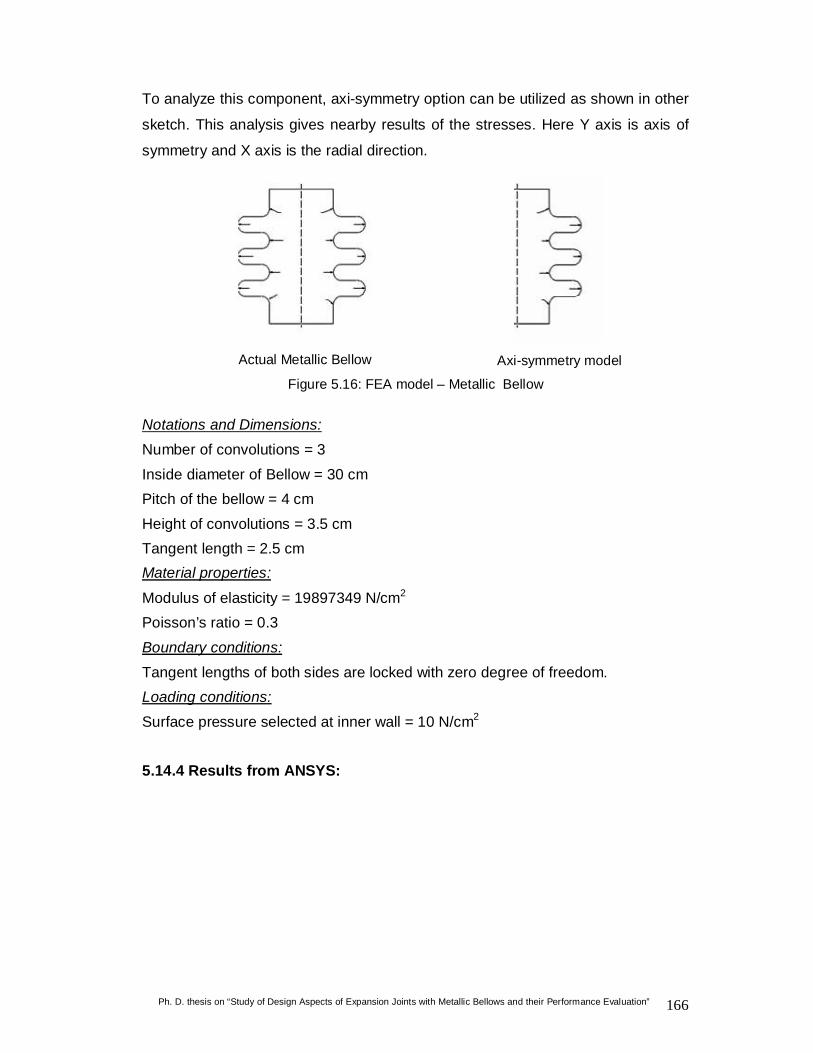
To analyze this component, axi-symmetry option can be utilized as shown in other

sketch. This analysis gives nearby results of the stresses. Here Y axis is axis of

symmetry and X axis is the radial direction.

Actual Metallic Bellow

Axi-symmetry model

Figure 5.16: FEA model – Metallic Bellow

Notations and Dimensions:

Number of convolutions = 3 Inside diameter of Bellow = 30 cm Pitch of the bellow = 4 cm Height of convolutions = 3.5 cm Tangent length = 2.5 cm Material properties:

Modulus of elasticity = 19897349 N/cm2 Poisson’s ratio = 0.3 Boundary conditions:

Tangent lengths of both sides are locked with zero degree of freedom. Loading conditions:

Surface pressure selected at inner wall = 10 N/cm2 5.14.4 Results from ANSYS:


Figure 5.17 : Circumferential stress of a bellow using 3 D shell element

1

MN

MX

-540.518

-420.286-300.054

-179.822-59.589

60.643180.875

301.107421.34

541.572

DEC 18 200910:31:44

ELEMENT SOLUTION

STEP=1SUB =1TIME=1SX (NOAVG)RSYS=0DMX =.092399SMN =-540.518SMX =541.572

Figure 5.18: Axi-symmetry analysis of a bellow

1

MN MX

XY Z

-498.444

-390.616 -282.789 -174.962 -67.135 40.693 148.52 256.347 364.175 472.002

DEC 18 2009 10:29:05

ELEMENT SOLUTION STEP=1 SUB =1 TIME=1 SX (NOAVG) RSYS=0 DMX =.456713 SMN =-498.444 SMX =472.002


5.15.5 FEA Results:

Table 5.6: FEA Results

Type of Analysis 2 D with axi-symmetry option

(solid element) N/cm2

3 D model Analysis (shell element)

N/cm2 Circumferential stress 3690 3532

Longitudinal stress 11610 11532

3690

11610

3460

11532

0

2000

4000

6000

8000

10000

12000

14000


Str

esse

s, N

/cm

2

Axi-symmetric 3 D shell

Figure 5.19: Graph showing comparison of Axi-symmetric and 3D approaches


1. The use of symmetry allows us to consider a reduced problem instead of

actual full size problem.

2. Modeling time is greatly reduced as geometry is simplified. The modeling of

axi-symmetry is in 2D plane.

3. For the axi-symmetry geometry model, number of nodes, number of elements

and number of equations are reduced compare to actual 3D analysis.

4. For the analytical solution, the order of the total stiffness matrix and total set

of stiffness equations are reduced considerably.

5. By taking advantage of symmetric geometry of the components, finite element

analysis becomes simple and fast.

6. 2D axi-symmetry analysis may be proven more accurate than an equivalent

3D analysis.


5.16 Practical considerations in FEA:

This exercise is carried out with an objective of considering various practical

aspects while performing Finite Element Analysis. A metallic bellow is considered

as a case study for the finite element analysis to study above stated objective. For

finite element analysis actual and full size component should not be considered

for the analysis, but various practical aspects should be taken in to account. There

are many practical aspects for FEA. They are planning of the analysis, choosing

type of model, use of symmetry, selecting critical area for maximum stresses,

meshing quality parameters, aspect ratio of elements, etc. A case study of bellow

is considered for Finite Element Analysis for validation of practical considerations.

The results are obtained using ANSYS software.

5.16.1 Practical Considerations in FEA:

1. Planning of the Analysis:

Before beginning the model some important decisions must be made by user. The

accuracy of results will depend on these decisions; hence they should be taken

very carefully.[B1]

a) Objectives of analysis:

b) Whether the full model or only portion of a physical system is sufficient.

c) Details to be included in the model.

d) Selection of elements

e) Meshing density

2. Choosing type of Model:

The finite element model may be categorized as being 2-D or 3-D, and as being

composed of point elements, line elements, area elements, or solid elements. Of

course, these can be used as combined different kinds of elements as required.

3. Use of Symmetry:

The appropriate use of symmetry will often expedite the modeling of a problem.

Three types of symmetry can be considered in the modeling[B3]. They are

axi-symmetry, repetitive (cyclic) symmetry or reflective symmetry. Appropriate use


of symmetry in the modeling allows designer to minimize the problem size instead

of the actual problem.

An axi-symmetry means object is symmetrical about its axis of revolution. The

object shapes may be either cylindrical or conical. The examples falls into this

category are rotors, cylinders, couplings, pistons, flywheels, electric bulb, bottles

or jar, glass, etc.

A repetitive symmetry means, similar pattern is repeating either on a straight line

or radial line. The examples in this type of symmetry are fins of an engine or worm

gear box, metallic bellow, teeth of a rack, spur gear etc.

A reflective symmetry means object is symmetrical about any one or two axis. It

appears like mirror image on other side of an axis. The examples in this type of

symmetry are rectangle plate with a circular hole, bearing cover, plastic container

etc. Figure 5.20 shows FEA model representation of bellows considering repetitive

symmetry.

Bellow with 3 convolutions

(Actual Problem)

Single convolution model

(FEA model representation)

Figure 5.20: Axi-symmetry and Repetitive Symmetry of Bellows


Number of convolutions, N = 3 Inside diameter of Bellow, Db = 30 cm Thickness of material, t = 0.05 cm Pitch of the bellow, q = 4 cm

Height of convolutions, w = 3.5 cm Tangent length, Lt = Lc = 2.5 cm Material properties:

Modulus of elasticity = 19897349 N/cm2 Poisson’s ratio = 0.3


Boundary conditions:

Tangent lengths of both sides are locked with zero degree of freedom. (Ux = 0, Uy = 0) Loading conditions:

Surface pressure selected at inner wall = 10 N/cm2 5.16.2 Modeling options:

Using axi-symmetric elements either three convolution model is required as

per geometry (figure 5.21). Instead of that, since convolutions are repeating at

regular pitch distance, one convolution model may be considered for the

analysis (figure 5.22). Results are shown in table 5.7.

Figure 5.21:

Axi-symmetric full size model Figure 5.22:

Axi-symmetric one convolution model

1

SEP 2 201007:55:58

ELEMENTS

Figure 5.23: Meshing in solid element


5.16.3 FEA Results:

Table 5.7: FEA Results Circumferential stresses, N/cm2 Longitudinal Stresses, N/cm2 Pressure

N/cm2 1 convolution model

3 D model 1 convolution model

3 D model

10 3730 3460 11020 11532

1

MN

MX

-185.707

-144.318-102.929

-61.54-20.15

21.23962.628

104.017145.406

186.796

SEP 2 201008:01:18

ELEMENT SOLUTION

STEP=1SUB =1TIME=1SXY (NOAVG)RSYS=0DMX =.006627SMN =-185.707SMX =186.796

Figure 5.24: ANSYS Results, Deformed shape

3730

11020

3460

11532

0

2000

4000

6000

8000

10000

12000

14000


Stre

sses

, N/c

m2

Repetitive Symmetry 3 D shell

Figure 5.25: Graph showing comparison of full model and single convolution model



1. In FEA analysis of bellow convolution pattern is repeating periodically at

equal distance (pitch). Hence, repetitive geometry concept may be

considered and one convolution sufficient for the stress analysis.

2. Bellow consist of symmetrical geometry, axi-symmetric element may be

used instead of 3 D shell (full size) model.

3. Axi-symmetry and repetitive geometry features can be used in combination

and finite element can be made simpler.

4. Here single convolutions results are compared to three dimensional full

size bellow. So, one convolution is sufficient for FEA. The variations in

results are within 20%.

5. Simple and smaller size of model provides higher accuracy in the results.

6. Practical aspects should be considered in modeling phase of finite element

analysis. Complicated component model can be simplified by use of

symmetry, elimination of least affected features etc. This will save modeling

and analysis time, as well as an accuracy of results will increases.


5.17 Comparison of Convolutions Shapes:

The bellow consists of optional convolution shapes like U, V, S, toroidal etc. as we

desire. Selection of each convolution shape will be based on designers’ choice, its

maximum pressure value and manufacturing facilities available. Each convolution

shape will have different effect on the performance of bellow. This exercise is

carried out with the objective that, study of various performance characteristics of

different shapes of convolution. Generally U shape, V shape, toridal shape are

mostly used in application. Hence these three are considered for the study with

Finite Element Analysis methodology. Figure 5.26 shows the comparative

geometry of these convolutions.

Figure 5.28: Shape and Dimensions of Convolutions


Number of convolutions, N = 1 Inside diameter of Bellow, Db = 300 mm = 30 cm Thickness of material, t = 0.05 cm Height of convolutions, w = 45 mm = 4.5 cm Tangent length, Lt = Lc = 25 mm = 2.5 cm Material properties:

Modulus of elasticity = 19728608 N/cm2 Poisson’s ratio = 0.3 Boundary conditions:


Tangent lengths of both sides are locked with zero degree of freedom. (Ux = 0, Uy = 0) Loading conditions:

Surface pressure selected at inner wall = 10 N/cm2 5.17.1 FEA Results:

U shape

V – shape

Toroidal shape

Figure 5.29 : Meshed model of shapes of convolutions

Table 5.8: FEA Results of U shape Convolutions

Pressure

N/cm2


N/cm2

Axial stress

N/cm2

Max. Stress intensity

N/cm2

1.0 5960 7030 13770

Table 5.9: FEA Results of V shape convolutions

Pressure

N/cm2


N/cm2

Axial stress

N/cm2


N/cm2

10 4990 9840 12540

Table 5.10: FEA Results of Toroidal shape convolutions

Pressure

N/cm2


N/cm2

Axial stress

N/cm2


N/cm2

1.0 4770 13450 14340


Graphs:

0

1000

2000

3000

4000

5000

6000

7000

U shape V shape Toroidal shape

Circ

umfe

rent

ial s

tres

s, N

/cm

2

Figure 5.30: Graph showing circumferential stress

0

2000

4000

6000

8000

10000

12000

14000

16000


Long

itudi

nal s

tres

s, N

/cm

2

Figure 5.31: Graph showing Longitudinal Stress


11500

12000

12500

13000

13500

14000

14500


Max

imum

str

ess

inte

nsity

, N/c

m2

Graph 5.32: Graph showing maximum stress intensity


1. The geometry of the convolution should have uniform shape, any sharp

change in geometry will create stress concentration effect and which will

leads to higher stress development.

2. In case of U shaped convolutions, circumferential stresses are at

maximum, while longitudinal stresses are at minimum level. This is

because of straight (perpendicular) convolution faces.

3. U shape convolution permits maximum axial displacement (movement)

because of root and crest flexibility. It is because of the vertical edges of

the convolutions, which permits higher deflection.

4. For toroidal shape convolutions, circumferential stresses are at minimum

level, while longitudinal stresses are at maximum level. This is due to its

spherical shape, and toroidal convolution can withstand higher amount of

stresses compared to other types of convolutions.

5. Toroidal shape do not permit higher axial deflection because of its spherical

shape.

6. V shaped convolution performs the stress level between U shape and

toroidal shape convolutions.


5.18 Structural and Thermal Analysis:

The design of bellows is very complex as it involves structural and thermal

aspects. Structural design point of view, the bellows should be flexible enough to

take up movements or deformations causes by pressure fluctuations. The bellows

are manufactured using minimum metal thickness in order to get higher deflection.

Here many times the bellows are deformed beyond elastic range of material,

hence prediction of stresses are very much critical. As the temperature of the

piping rises, the modulus of elasticity of the material is decreases; hence resulting

in the development of the higher stresses. The combined structural and thermal

aspect makes the design of bellows very much critical. The determination of an

acceptable design is further complicated by the numerous geometrical parameters

involved such as diameter, material thickness, and shape of convolutions, number

of convolutions, pitch, height of convolution, number of plies, etc.

5.18.1 Problem definition:

Notations Db = Inside diameter of the bellow = 30 cm

N = Number of convolution = 2

w = Height of convolution = 3.5 cm

q = Pitch of convolution = 4.0 cm

Lt = Lc = Tangent length = 2.5 cm

Thickness of materials = 0.05 cm

Number of ply of material = 1

Figure 5.33 Geometric Dimensions of a bellow

Bellows are made from sheet metal long tube (seam welded in longitudinal

direction). Then the convolutions are formed by any metal forming process using

dies. Generally U shape of convolutions is preferred. Figure 5.31 shows a bellow

with two convolution and single ply material. It shows the basic geometry of a

bellow.


5.18.2 Loading Conditions:

In actual practice the inside surface will be pressurized by fluid. Here we can

simplify the experiment by applying uniform pressure at inside surfaces of bellow.

Pressure at inside surface is taken as 10 N/cm2.

5.18.3 Boundary conditions:

As the expansion joints are fixed through the collar at both ends. The

displacement constraint is made fixed at both sides. The inside pressure will be

acting on cylindrical surface as well as convolution area. Tangent lengths at both

ends of bellows are covered by collars. Collars are made from comparatively thick

material, considering that the stresses are to be bared by convolutions only.

The tangent lengths at both ends are considered as zero degree of freedom as

these ends are welded to flanges and subsequently to long pipes.

Reference temperature is given at 273 K. Uniform temperature is at 3000K, 3500K,

4000K, 4500K, and 5000K are applied at for the stress analysis.

5.18.4 Results: Reference temperature: 273 K


Pressure N/cm2

Temperature 0K

Circumferential stress N /cm2

Axial stress N/cm2

Max. stress intensity N /cm2

10 300 3310 9470 12700

10 350 4980 26970 36220

10 400 7070 44460 59730

10 450 9170 61960 83250

10 500 11360 79460 106770


1

MNMX

XYZ

-1016

-797.902-579.785

-361.668-143.551

74.566292.683

510.8728.917

947.034

AUG 21 201023:12:21

ELEMENT SOLUTION

STEP=1SUB =1TIME=1SX (NOAVG)RSYS=0DMX =.019429SMN =-1016SMX =947.034

Figure 5.34: Longitudinal Stresses at uniform temperature 300 0K

5.18.5 Analytical Approach:

Strength of materials decreases with increase in temperature in case of steel. Its

modulus of elasticity is reduced because of thermal vibrations of the atoms in the

material, and hence to an increase in the average separation distance of adjacent

atoms. To consider this parameter, thermal expansion occurs based on its

coefficient of thermal expansion.

The linear coefficient of thermal expansion (Greek letter alpha) describes by

how much a material will expand for each degree of temperature increase.

The thermal expansion coefficient for a pipe is also a thermodynamic property of

that material.

δ = (ΔT) L

Where, δ is the elongation of pipe,

is the thermal expansion coefficient,

ΔT is the change in temperature, and

L is the initial length of the pipe.

The flexibility of a bellow is an important parameter for the designers. The actual

modulus of elasticity is not applicable for the design procedure, as the flexibility


increases because of its shell structure. The flexibility parameter is based on shell

parameter of a bellow. Many researchers has made attempts to find flexibility

parameter 'E

E for bellows. It depends on geometric parameters like n, b, h, R and

t of bellow.

Figure 5.35 : U shape geometry of a bellow

Shell parameter of bellow is λ = 2btR = 21

05.075.16 x = 0.83

Shell parameter λ = 'E

E , 0.83 = '

19728608E

, E’ = 23769407 N/cm2.

Formulation of stress relationship with reference to thermal expansion of bellow is

Elongation of pipe δ = (ΔT) L = 12.6 x 10-3 x (300 – 273) x 13 = 4.43 x 10-3 cm

Actual Modulus of elasticity, E’ = strainstress

Stress = E’ x strain = 23769407 x 13

1043.4 3x = 8100 N/cm2.

Using same procedure all values are computed in following table 5.12

Table 5.12: Analytical Results

Pressure N/cm2

Change in Temperature 0K

Axial Stresses N/cm2

10 300 – 273 = 27 8100

10 350 – 273 = 77 22780

10 400 – 273 = 127 37580

10 450 – 273 = 177 52380

10 500 – 273 = 227 67180


5.18.6 Graphs:

0

20000

40000

60000

80000

100000

120000

300 350 400 450 500

Temperature, K

Axi

al s

tres

ses,

N/c

m2

FEA Analytical

Figure 5. 36 : Comparison of FEA and Analytical Results


1. Longitudinal stresses developed in the bellows increases due to increase in

temperature, even though the pressure remains constant.

2. The analysis is based on linear relationship, and non linear mode may give

some variations in results. The elongation is based on thermal expansion of

bellow material.

3. Longitudinal (along axis) stresses and strains are always higher compared

to circumferential stresses because elongation takes place along the length

of pipe and bellow and stresses due to bending.

4. FEA results are validated with analytical approach for longitudinal stresses

developed in bellow. Finite element analysis using ANSYS gives near to

realistic results.


5.19 Stability Analysis:

Structural members, which are considerably long in dimensions compare to their

lateral dimensions, starts bending (buckling), when their compressive loading

reaches to some critical value. Buckling can be defined as the gross lateral

deflection of long columns at center sections. Buckling failure of structures mainly

depends upon slenderness ratio.

Expansion joints are used in the piping to take deviations occurring because of

temperature and pressure variations. These deviations may be axial, lateral and

combined. Bellow is a critical element of an expansion joint assembly. Bellows are

normally loaded with internal pressure along with elevated temperature depending

upon the applications. Design of bellow is very much critical as there are many

geometric parameters and many other affecting factors. The stresses developed

in the bellows are due to pressure and deflection. Some times bellows becomes

unstable because of excessive internal pressure. This kind of failure of bellows is

termed as ‘squirm’.

5.19.1 Squirm in Expansion Joints:

Expansion Joints Manufacturers Association (EJMA) has established the codes

for design of bellows considering buckling. This analytical approach is based on

Euler’s theory and gives near to realistic estimation of buckling load. This exercise

is an attempt to check the bellow for buckling failure using ANSYS finite element

method. The squirming phenomenon was first demonstrated by Haringx[2], who

showed pressure buckling of bellows was analogous to buckling of Euler strut. He

gave following relationship.

22'

lrIEP

Excessive internal pressure may cause a bellow to become unstable and squirm.

Bellows performance is depending on critical pressure. The pressure capacity is

decided based on squirm by keeping some factor of safety. Fatigue also depends

on squirm pressure. There are two basic types of squirm, column squirm and in-

plane squirm.


Figure 5.37 : Column Squirm Figure 5.38 : In-plane squirm

Column squirm is defined as a gross lateral shift of the middle section of the

bellow. In-plane squirm is defined as deflection occurred in individual

convolutions, parallel to the surface of bellow materials.

Squirm is associated with length to diameter ratio, called slenderness ratio.

According to slenderness ratio, bellows can be categorized in long or short

columns. Failure of column depends on the kind of column. Squirm is similar to

buckling of column under compressive load. Buckling failure consists of an elastic

and in-elastic deformation. Since bellows are made from thin sheet metal,

deformation of bellows exists in elastic and plastic region. Hence determination of

critical pressure is essential to avoid squirm failure.

Buckling analysis is a technique used to determine buckling load or critical load at

which a structure becomes unstable or buckle mode shapes - the characteristic

shape associated with a structure's buckled response. Eigenvalue buckling

analysis predicts the theoretical buckling strength (the bifurcation point) of an ideal

linear elastic structure. An eigenvalue buckling analysis of a column will match the

classical Euler solution[5]. However, imperfections and nonlinearities prevent most

real-world structures from achieving their theoretical elastic buckling strength.

Thus, eigenvalue buckling analysis often yields unconservative results. The non

linear analysis gives much accurate results.


5.19.2 Results:


Model Lb / Db ratio

No. of convolutions, N

Pitch, q (cm)

Buckling pressure (N/cm2)

1 5 5 8 22.70

ANSYS gives results 22.70 as limiting pressure for buckling to occur. Since

geometry of bellow is made in order to achieve maximum flexibility by shapes

and parameters like minimum thickness, height of convolutions, pitch of

convolutions, and convolutions formulations. These features are having

definite effect on the result. They are discussed below.


1. Euler’s equation gives satisfactory results for long columns only. ANSYS

buckling is based on Euler’s theory. Hence bellows geometry preferably in long

column should be considered for analysis.

2. Bellows material thickness is very less and it is having hollow structure, so

moment of inertia is very negligible, and hence results may not be accurate.

3. Bellows are having very high spring rate, because of its geometric features like

height of convolution, thin metal thickness etc. While Euler’s column is rigid.

Actually bellows possess more elasticity due to its geometry. Euler’s relation

includes elasticity based on property only.

4. Since EJMA suggests equation to calculate limiting pressure to avoid buckling.

It is an indirect way to make safe design. Equations suggested by EJMA

definitely give much more precise and safe design parameters.

5. Bellows may fail by squirm, if number of convolutions and pitch of bellow

parameters are selected on higher side. Bellows squirm pressure can be

evaluated and design pressure should be well within limit by keeping factor of

safety.

6. FEA for buckling analysis does not give accurate results because of its typical

shell type structure, hence not recommended for FEA.


5.20 Dynamic Analysis:

A steady flow of fluid is passing through the long pipes and expansion joints. The

fluid is passing at pressure higher than atmospheric, hence dynamic analysis of

expansion joint is necessary. Metallic bellows are supposed to be loaded with high

frequency and low amplitude vibrations. The piping system designer should take

care about vibration loads in the piping system. Designers can use external

damping device for reducing the vibration effects in the bellows. For turbulent flow

applications, inside sleeve arrangement must be provided in order to minimize the

vibration intensities. Piping elements are sturdy and rigid, while bellows tends to vibrate in the

convolution length because of pressurized fluid flow. The vibration intensities

depend on overall stiffness of bellow, type of fluid, and weight of bellow along with

fluid in the convolution region. The vibration intensities will be developed in axial

and lateral direction of bellow.

5.20.1 Harmonic Analysis using FEA:

A harmonic analysis, by definition, assumes that any applied load varies

harmonically (sinusoidally) with time. To completely specify a harmonic load, three

pieces of information are usually required: the amplitude, the phase angle, and the

forcing frequency range. Peak harmonic response occurs at forcing frequencies

that match the natural frequencies of your structure. Before obtaining the

harmonic solution, you should first determine the natural frequencies of your

structure by obtaining a modal solution

The amplitude is the maximum value of the load, according to type of problem.

The phase angle is a measure of the time by which the load lags (or leads) a

frame of reference.

Figure 5.37 shows the model created in the ANSYS environment. In solid type of

elements, axi-symmetric harmonic 4 node element is used to make model.


Geometric dimensions of bellow:

Inside diameter of bellow, Db = 16.9 cm.

Mean diameter of bellow, Dm = 18.63 cm.

Number of convolutions, N = 7

Number of plies, n = 1

Thickness of material = 0.04 cm.

Height of convolutions = 1.65 cm.

Pitch of convolutions, q = 2.60 cm.

Length of bellow, Lb = N x q = 18.20 cm.

Design pressure, P = 25 N/cm2

Figure 5.39 : Axi-symmetric model of bellow

5.20.2 Boundary conditions:

Bellows are always clamped from its tangent length at both ends with collar. All

(Ux and Uy) degree of freedom is locked at inner surface of tangent length.

5.20.3 Loading conditions:

Bellow is loaded with inside fluid surface pressure of 25 N/cm2. Room temperature

condition is assumed for the analysis.

5.20.4 Results:

Following results are derived from the Finite Element Analysis using ANSYS

platform.


Number of convolutions

Natural frequency (axial) Uy

Natural frequency (lateral) Ux

7 44 Hz 45 Hz


Graphs:

Figure 5.40 : Natural frequency in Axial direction

Figure 5.41 : Natural frequency in lateral direction


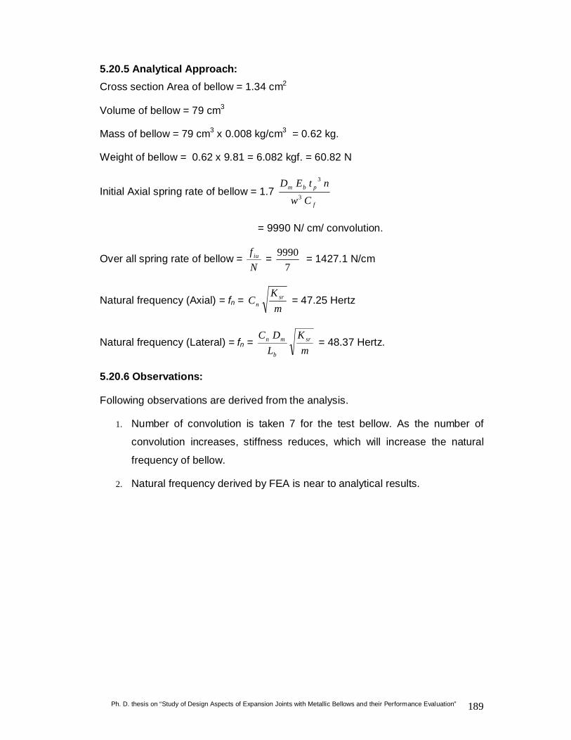
5.20.5 Analytical Approach: Cross section Area of bellow = 1.34 cm2

Volume of bellow = 79 cm3

Mass of bellow = 79 cm3 x 0.008 kg/cm3 = 0.62 kg.

Weight of bellow = 0.62 x 9.81 = 6.082 kgf. = 60.82 N

Initial Axial spring rate of bellow = 1.7 f

pbm

CwntED

3

3

= 9990 N/ cm/ convolution.

Over all spring rate of bellow = Nf iu =

79990 = 1427.1 N/cm

Natural frequency (Axial) = fn = m

KC sr

n = 47.25 Hertz

Natural frequency (Lateral) = fn = m

KLDC sr

b

mn = 48.37 Hertz.


Following observations are derived from the analysis.

1. Number of convolution is taken 7 for the test bellow. As the number of

convolution increases, stiffness reduces, which will increase the natural

frequency of bellow.

2. Natural frequency derived by FEA is near to analytical results.

5. finite element analysis of bellows -...

Documents