4th aiaa theoretical fluid mechanics meeting, 6–9 june ... · 4th aiaa theoretical fluid...

4th AIAA Theoretical Fluid Mechanics Meeting, 6–9 June 2005, Toronto, Ontario, Canada

Turbulent Marginal Separation and the

Turbulent Goldstein Problem

Bernhard Scheichl∗ and Alfred Kluwick†

Vienna University of Technology, A-1040 Vienna, Austria

A new rational theory of incompressible turbulent boundary layer flows having a largevelocity defect is presented on basis of the Reynolds-averaged Navier–Stokes equationsin the limit of infinite Reynolds number. This wake-type formulation allows for, amongothers, the prediction of singular solutions of the boundary layer equations under the actionof a suitably controlled adverse pressure gradient which are associated with the onset ofmarginally separated flows. Increasing the pressure gradient locally then transforms themarginal-separation singularity into a weak Goldstein-type singularity occurring in the slipvelocity at the base of the outer wake layer. Interestingly, this behavior is seen to be closelyrelated to (but differing in detail from) the counterpart of laminar marginal separationwhere the skin friction replaces the surface slip velocity. Most important, adopting theconcept of locally interacting boundary layers gives rise to a closure-free and uniformlyvalid asymptotic description of boundary layers which exhibit small closed reverse-flowregimes. Numerical solutions of the underlying triple-deck problem are discussed.

Nomenclature

A Displacement function (TD theory), Eqs. (98), (116)B, B1 Zeroth- and first-order coefficient in expansion of Us about χ = χ∗, Eqs. (125), (127)–(129)L Bubble lengthP Induced pressure, Eq. (100)s, x Shifted coordinates, Eq. (40)X, Y LD coordinates (TD theory), Eqs. (93), (112), (113)y Vertical UD coordinate, Eq. (105)X ,Y Transformed LD coordinates, Eq. (119)L, U Reference length, reference velocityA Displacement function (BL theory), Eq. (49)A+,− Numerical constants, Eqs. (25), (86)B Upstream slope of Us, Eq. (27)b Constant slope d∆/dx (self-preserving BL solution)C+ Numerical constant, Eq. (91)D Strength of perturbation of B, Eq. (32)F Stream function (self-preserving BL solution)f, f Stream functions (locally expanded BL solutions), Eqs. (19), (20), (55)F+,− Leading-order stream functions (locally expanded BL solutions), Eqs. (22), (24)G Stream function perturbation (locally expanded BL solutions), Eq. (79)g, g Stream function perturbations (locally expanded BL solutions) Eqs. (30), (34), (35)H Auxiliary functionh Surface metric coefficient

∗Postdoctoral Research Fellow, Vienna University of Technology, Institute of Fluid Mechanics and Heat Transfer, Resselgasse3/E322, A-1040 Vienna, Austria, e-mail: [email protected].

†Full Professor, Vienna University of Technology, Institute of Fluid Mechanics and Heat Transfer, Resselgasse 3/E322,A-1040 Vienna, Austria, e-mail: [email protected], Senior AIAA member.

Copyright c© 2005 by Bernhard Scheichl and Alfred Kluwick. Published by the American Institute of Aeronautics andAstronautics, Inc. with permission.

1 of 24

American Institute of Aeronautics and Astronautics Paper 2005-4936

I Intermittency factor, Eq. (12)k Surface curvaturem External flow exponent, Eq. (13)ms External flow exponent (self-preserving BL), Eq. (13)p Pressurer Exponent, Eq. (55)Re Reynolds number (globally defined), Eq. (1)s Local streamwise coordinates, Eq. (15)S, S Local streamwise LD coordinates, Eqs. (54), (125)T Reynolds shear stress (BL solution), Eq. (6)t, z Auxiliary variablesu′, v′ Velocity fluctuations in x- and y-directionU,P Local representations of ue, dp/dx, Eq. (14)u, v Velocity components in x- and y-directionU+ Numerical constant, Eq. (25)ue Surface slip velocity (external potential flow), Eq. (7)Us Surface slip velocity (BL solution), Eq. (10)us Surface slip velocity, Eq. (87)X, Y LD coordinates (BL theory), Eq. (42)x, y Natural coordinatesY BL coordinate, Eq. (5)

Subscripts

+,− Downstream and upstream (of s = 0 or s = 0) evolving formsD,R Detachment, reattachmentG,M Goldstein-type singularity, marginal-separation singularityi ith member in asymptotic seriesij jth member of ith member in asymptotic seriesijk kth member of jth member of ith member in asymptotic series

Conventions

Ψ , T LD representations (BL theory) of Ψ and T , Eq. (43)Us LD representation (BL theory) of Us, Eq. (47)

ψ, p UD perturbations of ψ, Eq. (106), and p, Eq. (107)Ψ , T LD representations (TD theory) of Ψ , Eqs. (112), (113), and T , Eq. (114)Us LD representation (TD theory) of Us, Eq. (121)q Notation to represent any quantity〈q〉 Reynolds-averaging of any quantity represented by q1a, 1b Oncoming near-surface flow regimes (BL theory)2 Downstream and upstream evolving main flow regimes (BL theory)I Lower deckII Main deckIII Upper deckBL Boundary layerIW Inner wakeLD Lower deckOW Outer wakeTD Triple-deckTST Transcendentally small termsUD Upper deck

Symbols

α Slenderness parameterβ Control parameter, Eq. (13)χ Coupling parameter, Eq. (92)χb Upper bound of χ, Eq. (94)δ BL thickness

2 of 24


ℓ Mixing length, Eq. (8)ǫ Bifurcation parameter (redefined), Eq. (41)η, η Similarity variables based on s, Eq. (18), and s, Eq. (76)η, η, η Similarity variables, Eqs. (29), (34), (54)γ Bifurcation parameter, Eq. (15)κ V. Karman constant, Eqs. (11), (131)λ, µ Invariance parameters, Eq. (119)ω Exponent, Eqs. (30), (35)φ Scaling function, Eqs. (34), (36)ψ Stream functionρ, ϑ Polar coordinates, Eq. (70)ρ, ϑ Polar coordinates (UD), Eq. (109)σ TD length scale, Eq. (93)τ Surface friction, Eq. (131)θ Heaviside functionν Kinematic viscosity∆ BL thickness (BL solution), Eq. (6)Γ Upstream limit of Us, Eqs. (93), (117), (123)Λ Strength of induced pressure, Eqs. (95), (100), (114)Ω EigenvalueΨ Stream function (BL solution), Eq. (6)ξ BL coordinate related to ∆, Eq. (12)ζ Auxiliary variable

Superscripts

∗ Onset of separation

I. Introduction

A Tribute to the Work of Professor Dr. David Walker on Turbulent Boundary Layers

The method of matched asymptotic expansions has undoubtedly proven very successful not only in gaininga profound understanding of laminar high-Reynolds-number flows in many aspects but also in providing

a rational framework for a comprehensive treatment of turbulent shear layers. It is the merit of DavidWalker to as one as the first having elucidated the modern and fruitful asymptotic formulation of theclassical two-dimensional two-tiered turbulent boundary layer structure which is essentially based on theassumption of an asymptotically small streamwise velocity defect with respect to the external free-streamflow, see the extensive contribution Ref. 1. For an extension to the three-dimensional case the reader isreferred to Ref. 2 and Ref. 3, and a summary is also given in Ref. 1. In contrast to earlier treatments ofwall-bounded turbulent shear flows, in his pioneering analysis the local skin friction velocity serves as theprincipal perturbation parameter. In turn, the well-established logarithmic law of the wall appears as thelimit far from the surface of the leading-order streamwise velocity distribution inside the viscous wall layer.Hence, the whole information needed for the further analysis of the outer velocity defect layer is subsumedin a single term in an elegant manner. We note that this formulation was also adopted by Gersten4,5 and,more recently, in the further developments by the present authors.6,7

Moreover, it must be emphasized that David Walker was substantially involved in providing the initialsteps towards an understanding of the very complex turbulent near-wall dynamics by investigating theunsteady Navier–Stokes equations in the high-Reynolds-number limit.1,8–10

Despite the undeniable progress, where much of it must be attributed to David Walker, asymptoticmethods have contributed towards an understanding of the fundamental physics of wall-bounded turbulentshear flows, a fully self-consistent theory describing turbulent boundary layer separation in the limit of highReynolds number is not available at the moment. In particular, the literature lacks a rational descriptionof the, from an engineering point of view, very important case of separation from a smooth surface whichis caused by a smooth adverse pressure gradient, imposed by the external flow. In laminar boundary layertheory this type of separation is commonly referred to as marginal separation as the boundary layer mayexhibit a closed reverse-flow regime at its base if the pressure gradient is properly chosen. This theory was

3 of 24


developed independently by Ruban11,12 and by Stewartson et al.,13 also cf. Ref. 14. However, a systematicapproach to its turbulent counterpart has been hampered severely by the fact that, generally spoken, turbu-lent boundary layers are known to be less prone to separate than the corresponding laminar ones, owing tothe enhanced wall shear stress. More specifically, the classical small-defect formulation is seen to withstanda smooth adverse pressure gradient as the wall shear stress remains constant in the high-Reynolds-numberlimit. Furthermore, the velocity defect solution in the outer main layer is characterized by linearized convec-tive terms in leading order, which indicates that it does not terminate in a singularity during downstreamevolution. As a matter of fact, this property is demonstrated numerically by the preliminary work Ref. 6 forthe present investigation. Additionally, the study of turbulent separation past a blunt body by Neish andSmith15 serves as a further strong hint that the classical description of a turbulent boundary layer exposedto a smooth adverse pressure gradient predicts firmly attached flows which do not separate at all (apart fromthe inevitable flow detachment close to the rear stagnation point as it is the case in the situation consideredin Ref. 15) in the limit of high Reynolds number.

The first systematic approach, however, to tackle the challenging problem of pressure-induced turbulentseparation from an asymptotic viewpoint was carried out by Melnik.16,17 He proposed a primary expansionof the flow quantities in terms of a small parameter, denoted by α, which measures the slenderness of theboundary layer and is contained in all commonly employed shear stress closures and/or fixed by experiments.Most important, its value appears to be essentially independent of the Reynolds number as the latter maytake on arbitrarily large values. By assuming a (non-dimensional) velocity defect of O(1) in the mainbody of the boundary layer, that strategy is seen to provide a powerful tool for constructing a rational noveldescription of turbulent boundary layers, which predicts wake-type wall-bounded flows in the limit of infiniteReynolds number and even allows for the treatment of marginal separation.

Among others, a highlight of Melnik’s analysis is the prediction of a square-root singularity encounteredby the slip velocity at the base of the outermost wake region of the boundary layer as separation is approacheddue to the occurrence of an Eulerian flow stage close to the surface. This result may be regarded as theturbulent counterpart to the celebrated Goldstein singularity18,19 in laminar boundary layer theory wherethe slip velocity is replaced by the wall shear stress. Rather remarkable, however, it has recently beenshown20 that the pressure gradient can be controlled in a way such that the Goldstein-type singularityeventually disappears: then the slip velocity decreases regularly, vanishes in a single point but increasesrapidly immediately further downstream, giving rise to an abrupt acceleration of the flow near the surface.In turn, this situation is associated with turbulent marginal separation.

Unfortunately, Melnik’s theory16,17 is not only incomplete as it does not give a hint how to surmount thatseparation singularity within the framework of the Reynolds-averaged Navier-Stokes equations but remainsconceptually unsatisfactory, also for a number of additional reasons:

(i) In definite contrast to the primary premise of α being independent of the globally defined Reynoldsnumber Re as Re → ∞, the approach implies that α1/2 lnRe = O(1) in order to account for the well-known logarithmic near-wall portion of the streamwise velocity holding upstream of separation.

(ii) The formation of a square-root singularity in the slip velocity which also includes the effects due tothe Reynolds shear stress gradient must be taken into account, in principle. Therefore, if the Eulerianlimit holds indeed (independent of a specific closure), the theory lacks an explanation why such a moregeneral form of a singularity does not occur.

(iii) It remains unclear how far the asymptotic flow structure and the main results depend on Melnik’schoice of the algebraic eddy-viscosity-based closure for the Reynolds shear stress in the outer wakeregime.

The novel theory to be presented here is based on Melnik’s formulation of turbulent boundary layers havinga large velocity defect, strikingly contrasting the classical asymptotic theory. Most important, however, italso copes with the issues (i)–(iii). In the subsequent analysis we concentrate on the case α≪ 1 at infiniteReynolds number, formally written as 1/Re = 0.

The paper is organized as follows: in § II the essential basic assumptions underlying the theory and theirimplications are presented. In § III we give a short survey of the numerical study of a boundary layer drivenby a controlled pressure gradient towards marginal separation and the local analysis of the flow near thepoint of vanishing slip velocity. Such an investigation has already been presented in Ref. 20 and will beoutlined more extensively in Ref. 21. The key results of the contribution are provided by § IV where we focus

4 of 24


on the local interaction of the marginally separating boundary layer with the induced external irrotationalflow. As a highlight, akin to the laminar case,12,13 a fundamental equation governing turbulent marginalseparation, which is independent of a specific shear stress closure, is derived, and its solutions are discussed.

II. Motivation and Problem Formulation

A. Governing Equations

We consider a nominally steady and two-dimensional fully developed turbulent boundary layer driven by anincompressible and otherwise non-turbulent bulk flow along a smooth and impermeable solid surface, beinge.g. part of a diffuser duct. Let x, y, u, v, u′, v′, and p denote plane natural coordinates, respectively, alongand perpendicular to the surface given by y = 0, the time-mean velocity components in x- and y-direction,the corresponding turbulent velocity fluctuations, and the time-mean fluid pressure. These quantities arenon-dimensional with a reference length L characteristic for the mean velocity variation of the bulk flowalong the surface (and the surface geometry), a reference value U of the surface slip velocity due to theprescribed inviscid and irrotational external free stream flow, and the uniform fluid density. The (constant)kinematic fluid viscosity ν and L, U then define a suitable global Reynolds number Re, which is taken to belarge,

Re = U L/ν → ∞. (1)

We furthermore introduce a stream function ψ by

∂ψ/∂y = u, ∂ψ/∂x = −h v, h = 1 + k(x) y. (2)

Here k(x) = O(1) is the non-dimensional surface curvature, where the cases k < 0, k = 0, and k > 0 refer toa, respectively, concave, plane, and convex surface. Adopting the usual notation for the turbulent stresses,the dimensionless time- or, equivalently, Reynolds-averaged Navier–Stokes equations then read

h(∂ψ

∂y

∂

∂x− ∂ψ

∂x

∂

∂y

)∂ψ

∂y− k

∂ψ

∂x

∂ψ

∂y= −h∂p

∂x− h

∂〈u′2〉∂x

− ∂ h2〈u′v′〉∂y

+O(

Re−1)

, (3)

(∂ψ

∂x

∂

∂y− ∂ψ

∂y

∂

∂x

)( 1

h

∂ψ

∂x

)

− k(∂ψ

∂y

)2

= −h∂p∂y

− ∂ h〈v′2〉∂y

− ∂〈u′v′〉∂x

+ k〈u′2〉 +O(

Re−1)

. (4)

Herein the terms of O(Re−1) refer to the divergence of the viscous stresses, which are presumed to benegligibly small compared to the Reynolds stresses throughout the boundary layer with the exception of aviscous sublayer adjacent to the surface.

B. A Novel Wake-like Limit of Wall-Bounded Turbulent Shear Flows

A new approach to turbulent boundary layers has been developed in order to provide an appropriate asymp-totic concept for a description of marginally separated flows. This theory is essentially founded on three keyassumptions (which, although seeming plausible, nevertheless have to be validated empirically):

(i) Both the velocity fluctuations u′ and v′ are of the same order of magnitude in the limit Re → ∞, sothat all Reynolds stress components are scaled equally in the whole flow field. This requirement isinvoked quite frequently in the further analysis but will not be addressed again then.

(ii) As the basic property of the flow and already mentioned in the introduction, the streamwise velocitydeficit in the main part of the boundary layer, where the Reynolds shear predominates over molecularshear, is a quantity of O(1).

(iii) The distance y = δ(x) from the surface defines the time-mean outer edge of the boundary layer. Thisis in agreement with the observation of a rather sharp fluctuating outer edge of the time-dependentfluid motion.

5 of 24


1. Leading-Order Boundary Layer Problem

As a first consequence of the items (i)–(iii), inspection of the equations of motion (3) and (4) suggests ashear layer approximation, where the slenderness of the associated boundary layer is measured by a smallpositive parameter, denoted by α≪ 1. We, therefore, anticipate inner expansions

y = αY, (5)

ψ,−〈u′v′〉, δ = αΨ(x, Y ), T (x, Y ), ∆(x) +O(α2), (6)

p− p0(x) = O(α) where dp0/dx = −ue due/dx = O(1). (7)

Herein ue(x) denotes the surface velocity imposed by the external potential bulk flow. Then, the main flowregime of the boundary layer is governed by the boundary layer equation

∂Ψ

∂Y

∂2Ψ

∂Y ∂x− ∂Ψ

∂x

∂2Ψ

∂Y 2= ue

due

dx+∂T

∂Y, T = ℓ2

∂2Ψ

∂Y 2

∣

∣

∣

∣

∂2Ψ

∂Y 2

∣

∣

∣

∣

, (8)

where the latter relationship defines the mixing length ℓ. Equation (8) is subject to the wake-type boundaryconditions

Ψ(x, 0) = T (x, 0) = 0,∂Ψ

∂Y

(

x,∆(x))

− ue(x) = T(

x,∆(x))

= 0. (9)

The requirements to be satisfied at the boundary layer edge given by Y = ∆(x) reflect the patch with theirrotational external flow, and the conditions holding at the base of the outer wake arise from the matchwith the α- and Re-dependent sublayers. These are not considered here in detail but will be discussed inRef. 21 and outlined briefly in § II.B.2.

Note that the solution in the outer wake region comprising most of the boundary layer is completelydetermined by Eqs. (8) and (9). As an important consequence arising from the boundary conditions (9), asolution of Eq. (8) gives rise to an in general non-vanishing slip velocity

Us =∂Ψ

∂Y(X, 0). (10)

We expect non-trivial solutions of Eqs. (8) and (9), i.e. wake-type solutions having Us 6≡ ue and T 6≡ 0. Inother words, the simple Eulerian time-mean limit of the Navier–Stokes equations which implies ∂Ψ/∂Y ≡ ue(x)is disregarded.

2. Does the Boundary Layer Thickness Depend on Re?

Highly remarkably, dimensional reasoning suggests that the last of the boundary conditions (9) is fullyequivalent to a negation of this question as far as the limit Re → ∞ is concerned. Then the last statementin the foregoing paragraph implies that the Reynolds equations (3), (4) admit a further limit apart fromthe pure Eulerian one, such that the slenderness parameter α remains indeed finite even in the formal limit1/Re = 0.

The rationale can be subsumed as follows:21 Dimensional arguments strongly indicate that the mixinglength satisfies the well-known v. Karman’s near-wall law. Using the present notation, it is written as

ℓ ∼ κY/α1/2, (11)

where κ denotes the v. Karman constant. The relationship (11) holds in the overlap conjoining the fullyturbulent part of the boundary layer and the viscous sublayer, where molecular shear has the same magnitudeas its turbulent counterpart.7 Since Eq. (11) clearly prevents matching the flow quantities in the main part ofthe boundary layer and the viscous sublayer, at least one additional intermediate layer has to be introducedwhich provides the linear decay of the mixing length predicted by Eq. (11) at its base. In other words,the flow in the outer main layer and, as the most important consequence, the boundary layer thickness δare unaffected by the surface friction and thus by the strongly Reynolds-number-affected flow close to thesurface, at the least to leading order. Therefore, the scaling parameter α is seen to be independent of Re asRe → ∞, and the shear stress tends to zero as Y → 0.

Moreover, the mixing length ℓ is supposed to admit a finite limit for Y → 0. In turn, it is a quantityof O(1) in both the main and the intermediate layer the thickness of which then is of O(α3/2). As α does

6 of 24


not depend on Re, even the Reynolds shear stress in the latter region does not match the asymptoticallyconstant shear stress in the viscous near-wall region. Thus, both flow regimes are identified as an outer andinner wake layer, respectively. It is interesting to note that the asymptotic structure of the boundary layerthen closely resembles that of a turbulent free shear flow which was investigated by Schneider.22 One majorexception is the surface effect expressed by Eq. (11), giving rise to a square-root behavior of u,6,7 which hasoriginally been established to hold on top of the viscous sublayer in case of a separating boundary layer,see e.g. Ref. 4. Hence, for finite values of Re a further layer emerges between the viscous sublayer and theinner wake region. Therein, the Reynolds shear stress matches the wall shear stress but varies linearly withdistance from the surface.6,7 In view of the subsequent analysis, however, it is sufficient to consider theouter wake layer only.

III. Singular Solutions of the Boundary Layer Equations

Since it provides the motivation of the present analysis, it is useful to present a brief survey of Ref. 20.In this connection we stress that we are interested primarily in particular solutions of Eqs. (8) and (9) whereUs(x) vanishes locally, indicating the onset of separation.

A. Weakly Singular Numerical Solutions

In order to complete the turbulent boundary layer problem, Eqs. (8) and (9) are supplemented with thesimple mixing length model

ℓ = I(ξ)∆(x), I(ξ) = 1/(1 + 5.5 ξ6), ξ = Y/∆(x), (12)

where the well-known intermittency factor I(ξ) by Klebanoff23 accounts for the decrease of the mixing length(and thus for an improved flow prediction) near the boundary layer edge, cf. the experimental data presentedin Ref. 24. In fact, calculations employing the classical almost constant mixing length distribution in theoutermost region4 yield a slightly slower decay of the streamwise velocity near y = ∆(x) and appear tooverestimate the boundary layer thickness function ∆(x).

Numerical solutions of the problem posed by Eqs. (8), (9), and (12) were obtained for retarded externalflows which are assumed to be controlled by two parameters ms and β, which e.g. characterize the diffusershape, by specifying distributions of ue of the form

ue(x;ms, β) = (1 + x)m(x; ms, β),m

ms= 1 +

β

1 − βθ(2 − x)

[

1 − (1 − x)2]3, ms < 0, 0 ≤ β < 1. (13)

Here θ(t) denotes the Heaviside function where θ = 0 for t < 0 and θ = 1 for t ≥ 0. It is expected, however,that other choices neither of ue(x) nor of the mixing length closure (12) will affect the behavior of the solutionnear the location where Us = 0 significantly. We also note with respect to the imposed velocity distribution(13) that in the case β = 0, i.e. m ≡ ms, the boundary layer equations (8) and (9) admit self-similar solutionsΨ = ∆F (ξ), ∆ = b (1 + x), where b = const and the position x = −1 defines the virtual origin of the flow,if ms > −1/3. Then both the linear growth b of the boundary layer thickness and the exponent ms arefunctions of F ′(0), leading to a slip velocity Us ∝ (1 + x)mF ′(0).4–6 These solutions were used to provideinitial conditions at x = 0 for the downstream integration of Eqs. (8), (9), and (12) with ue given by Eq. (13).The calculations were started by prescribing a rather small velocity defect characterized by F ′(0) = 0.95 atx = 0, which in turn yields b

.= 0.3656 and ms

.= −0.3292. Computations were then carried out for a number

of positive values of the control parameter β. Inspection of Eq. (13) shows that the exponent m then varieswithin the range 0 < x < 2 and thus causes an additional deceleration of ue there. The key results whichare representative for the responding boundary layer are displayed in figure 1 (a).

If β is sufficiently small, the distribution of Us is smooth, and Us > 0 throughout. However, if β reachesa critical value βM

.= 0.84258, the surface slip velocity Us is found to vanish at a single location x = xM but

is positive elsewhere. A further increase of β provokes a breakdown of the calculations, accompanied withthe formation of a weak singularity slightly upstream at x = xG. An analogous behavior is observed for theboundary layer thickness ∆, which is smooth in the sub-critical case β < βM , exhibits a rather sharp peak forβ = βM at x = xM , and approaches a finite limit ∆G in an apparently singular manner in the super-criticalcase β > βM .

7 of 24


0.12

0.1

0.088

7

6

5

4

0.9

0.06

0.04

0.02

0.95 1 1.15 1.2 1.25 1.31.05

9

10

0

Us

Us

∆

∆∆00 = ∆(xM )∆G = ∆(xG)

xxG xM

(a)

4

3

2

1

0

−1

2520151050−10−15−20 −5

A

AG = A(XG)

Us

XXG

(b)

Figure 1. Critical (solid), sub- (dashed), and super-critical (dotted) boundary layer solutions: (a)β ≈ βM

.= 0.84258 (solid), β = 0.8422 (dashed), β = 0.8428 (dotted), (b) canonical representation.

Following the qualitatively similar behavior of the wall shear stress which replaces the slip velocity in thecase of laminar boundary layers,11 here the critical solution is termed a marginally separating boundary layersolution. However, in vivid contrast to its laminar counterpart,11 it is clearly seen to be locally asymmetricwith respect to the critical location x = xM where it is singular. Moreover, the turbulent solutions appearto be highly sensitive numerically to very small deviations from β = βM as x− xM → 0−. As will turn outin the following, these closely related properties reflect the basic mechanism governing the flow in the limitsx→ xM and β → βM , which is vastly different from the laminar case.

B. The Marginal-Separation Singularity

To study the local flow behavior near x = xM both the outer-edge velocity ue and the pressure gradientdp0/dx given by Eq. (7) are Taylor-expanded as

ue = U00 + sU01 + γU10 + · · · , dp0/dx = P00 + γP10 + · · · , P00 = −U00U01, P10 = −U10U01, (14)

where the perturbation parameters s and γ are defined by

s = x− xM → 0, γ = β − βM → 0. (15)

At first we focus on the critical case γ = 0. Then both the quantities Ψ and ∆ are seen to assume a finitelimit,

Ψ(x, Y ) → Ψ00(Y ), ∆(x) → ∆00 as s→ 0, (16)

see figure 1 (a) and figure 2 on page 10, and, in agreement with the considerations pointed out in § II.B.2,inspection of Eq. (12) indicates the important relationships

ℓ(x, Y ) → ℓ0(Y ) as s→ 0, ℓ0 → ℓ00 = O(1) as Y → 0. (17)

Equation (17) provides the only empirical parameter ℓ00 entering the local analysis.We furthermore note that in both the main regions 2− and 2+ where Y = O(1), see figure 2 on page 10,

the flow is Eulerian to leading order as s→ 0−. However, the momentum balance (8) including also theReynolds stress gradient is fully retained in the regions 1a− and 1+ where the wall coordinate

η = Y/(ℓ2/300 |s|1/3) (18)

is a quantity of O(1). There the following expansions are suggested in, respectively, the upstream and the

8 of 24


downstream case,

s→ 0− :Ψ

ℓ2/300 P

1/200

= (−s)5/6f0−(η) + (−s)4/3f1−(η) + · · · , (19)

s→ 0+ :Ψ

ℓ2/300 P

1/200

= s5/6f0+(η) + · · · , (20)

and the resulting boundary value problem for f0∓(η) reads

1/2 f ′20∓ − 5/6 f0∓f′′0∓ = ±1 ∓ (f ′′20∓)′,

η = 0 : f0∓ = f ′′0∓ = 0, η → ∞ : f0∓ = O(η5/2), (21)

where the upper and lower signs refer to the cases s→ 0− and s→ 0+, respectively. The conditions at η = 0follow from the wake-type boundary conditions (9), and the requirement for η → ∞ reflects the match withthe flow regimes 2− and 2+, see figure 2 on the following page, where the relations (16) and (17) hold. Itwill be shown in Ref. 21 that in the upstream case the problem (21) has only the obvious solution

f0− = F−(η) = 4/15 η5/2, (22)

which expresses a balance between the Reynolds shear stress gradient and the adverse pressure gradient atthe surface for vanishing convective terms. In turn, the match with the marginally separating profile Ψ00(Y )of the stream function implies

Ψ00 ∼ 4

15

P1/200

ℓ00Y 5/2, Y → 0, (23)

and f0+ ∼ F−(η) as η → ∞. However, in the case s→ 0+ a combined analytical and numerical investigationreveals a single (strictly positive) non-trivial solution that has to be calculated numerically,21

f0+ = F+(η), η → ∞ : F+ = 4/15 (η +A+)5/2 + TST, (24)

where TST means transcendentally small terms. It is found that

A+.= 1.0386, U+ = F ′

+(0).= 1.1835. (25)

As a result of the leading-order analysis, turbulent marginal separation is seen to be associated with apurely regular behavior of the flow upstream of s = 0 as expressed by the higher-order term in the expansion(19). Substitution into Eq. (8) yields

f1− = B(

η +η4

180

)

, B > 0, (26)

where the constant B characterizing the slope dUs/ds ∼ −BP 1/200 of the linearly decreasing slip velocity in

the limit s→ 0− must be determined numerically from the oncoming flow, cf. the upstream distribution ofUs in figure 1 (a). That is, the flow is locally governed by the eigensolutions f0−(η), f1−(η), and f0+(η), sothat

s→ 0− : Us/P1/200 = −Bs+ · · · , (27)

s→ 0+ : Us/P1/200 = U+ s

1/2 + · · · , (28)

Hence, the existence of the non-trivial downstream solution turns out to be responsible for the (infinitely)strong acceleration of the flow immediately downstream of the location s = 0 due to the irregular behavior ofUs, see Eq. (28). In turn, the convective part in Eq. (8) evaluated at Y = 0, given by Us dUs/dx, exhibits ajump at s = 0 from 0 to the value P00U

2+/2 in leading order. By adopting the numerical value P00

.= 0.02272,

the downstream asymptote (28) is plotted as a thin solid line in figure 1 (a).The fact that convection does not vanish necessarily at the surface Y = 0 not only causes the inher-

ently nonlinear downstream behavior, governed by Eq. (21), in contrast to the theory of laminar marginalseparation,11,12 but also gives rise to a fundamentally different analysis of the perturbed case γ 6= 0.

9 of 24


I

I+

II

1a−

1b−

1+

2−2+

ss

YY = ∆(x)

∆ = ∆00

∼ ǫ

∼ ǫ2

Figure 2. Asymptotic splitting of the oncoming (subscripts −) and downstream evolving (subscripts +) bound-ary layer flow, double-deck structure (lower deck I, main deck II). The case γ 6= 0 is sketched using solid lines,whereas the limiting structure for γ = 0 characterizing marginal separation is drawn using dashed lines partly.The flow regimes indicated by dotted lines are seen to behave passively and are thus not considered in thetext.

C. Bifurcating Flow for γ 6= 0

1. Transcendentally Growing Eigensolutions

The contributions given by Eqs. (22) and (26) to the expansion (19) become of the same order of magnitudeat distances s where the new variable

η = η/(−B2s)1/3 (29)

is a quantity of O(1). This situation forces a further sublayer 1b−, see figure 2, where the gradients of theReynolds shear stress and the pressure dominate over convection. Furthermore, the most rapidly downstreamgrowing perturbations possible are assumed to originate in this layer as their s-derivatives may becomeasymptotically larger than the disturbances itself there, such that convection comes into play again veryclose to the surface. Also, these perturbations must be due to the terms proportional to γ in Eq. (14). Theseconsiderations and inspection of the boundary layer equations (8) and (9) suggest the following expansionin region 1b−,

Ψ

ℓ2/300 P

1/200 (−Bs)5/3

= F−(η) + η + · · · − γ exp(

ω(s))

g(η) + · · · , ω(s) = − Ω

B2s+ o(1/s), Ω > 0. (30)

The higher-order contributions to the exponent ω(s) must be determined by analyzing the higher-order termsin the expansion (30) by means of the Fredholm alternative in order to investigate the consecutive inhomo-geneous problems.21 The eigenvalue Ω, however, is fixed by the solution of the leading-order eigenvalueproblem for the eigensolution g(η), found by linearization of Eqs. (8) and (9),

Ω [(2/3 η3/2 + 1)g′ − η1/2g] = 2(η1/2g′′)′, g(0) = g′′(0) = 0, g′(0) = D > 0. (31)

Here the unknown constant D is assumed to be fixed by the oncoming flow, such that the expansion (27) isperturbed according to

Us/P1/200 = −Bs

[

1 − γD exp(

ω(s))]

+ · · · . (32)

10 of 24


A numerical study shows that problem (31) allows for a solution g(η) having sub-exponential growth forη → ∞ solely in the case Ω = 1/3. Moreover, only in that case the solution of problem (31) has been foundanalytically. It reads

g(η)/D =2

3η exp(−z) +

(2

9

)1/3(2

3η3/2 + 1

)

∫ z

0

t−1/3 exp(−t) dt, z =2

9η3/2. (33)

In turn, the associated perturbation in expansion (30) provokes also exponentially small disturbances in theflow regimes 1a− and 1b−, respectively, and the distribution of the boundary layer thickness ∆(x).

We complete the analysis of eigensolutions which grow transcendentally as s→ 0− by scrutinizing thepossibility of the generation of eigensolutions which originate in a region located even closer to the surfacethan is the flow regime 1b−, see figure 2 on the preceding page. This is accomplished by the introduction ofthe new local variables

η = η/φ(−s), g(η) = g(η), (34)

which are assumed to be quantities of O(1). The latter relationship in Eq. (34) expresses the match of the(for the present analysis here unknown) shape function g(η) of the respective perturbation in region 1b−with that considered here, denoted by g(η). Independent of the specific choice of the (positive) functionφ(−s), substitution of the coordinate stretching (34) into the boundary layer equations Eqs. (8) and (9) isseen to be consistent with the generalized form

Ψ

ℓ2/300 P

1/200 (−Bs)5/3φ

= η + φ3F−(η) + · · · − γ exp(

ω(s))

g(η) + · · · , 1

ω(s)→ 0+ as s→ 0−, (35)

of the expansion (30). In the limitφ(−s) → 0+ as s→ 0− (36)

under consideration the balance between the perturbations of O(γ) of the convective terms and the Reynoldsstress gradient requires to write

ω = ω0(s) + o(ω0), s→ 0−, (37)

where φ can always be scaled such that

ω′0(s) = (Bs)−2 φ(−s)−3, s→ 0−. (38)

Then the associated disturbances having a growth rate ω′(s) given by Eqs. (37) and (38) which is strongerthan that implied by the expansion (30) are found to be governed by a reduced form of the problem (31).Integrated once, it reads

g = 2 η1/2g′′, g(0) = g′′(0) = 0, g′(0) > 0. (39)

However, the solution of problem (39) exhibits exponential growth for η → ∞. Consequently, no eigensolu-tions with a growth rate stronger than that given by Eq. (30) are generated.

2. Canonical Boundary Layer Solutions

The expansion (30) ceases to be valid within region I, the so-called lower deck, see figure 2 on the previouspage, where −B2s ∼ Ω/ ln(1/γ). It then is convenient with respect to the further analysis to introduce thecoordinate shift

s = s+ ǫ/B, x = x+ ǫ/B, (40)

see figure 2, by considering the limit

ǫ = −Ω/(B ln |Dγ|) → 0, Ω = 1/3. (41)

Substitution of the variables

X =s

ǫ2, Y =

Y

(ℓ00ǫ)2/3, Ψ(X, Y ) =

Ψ

ℓ2/300 P

1/200 ǫ5/3

, (42)

11 of 24


which are quantities of O(1) in the flow regime I, into Eqs. (8) and (9) yields to leading order the reduced,i.e. canonical, equations

∂Ψ

∂Y

∂2Ψ

∂Y ∂X− ∂Ψ

∂X

∂2Ψ

∂Y 2= −1 +

∂T

∂Y, T =

∂2Ψ

∂Y 2

∣

∣

∣

∣

∂2Ψ

∂Y 2

∣

∣

∣

∣

, (43)

subject to the boundary conditions

Y = 0 : Ψ = T = 0, (44)

Y → ∞ : ∂T /∂Y − 1 → 0, (45)

X → −∞ : Ψ → F−(Y ) + Y − sgn(γ) exp(X/3) g(Y ). (46)

It is furthermore useful to define the rescaled slip velocity

Us =∂Ψ

∂Y(X, 0), (47)

which serves to expand Us,

Us = ǫP1/200 Us(x) + · · · , (48)

and the displacement functionA(X) = lim

Y →∞

(T − Y ). (49)

By matching with the flow in the main deck II, see figure 2 on page 10, one then obtains

Ψ = Ψ00(Y ) + ǫ2/3 ℓ2/300 A(X)Ψ ′

00(Y ) + · · · + (ǫ− ǫ2BX)Ψ01(Y ) + · · · . (50)

In turn, applying the boundary conditions Eq. (9) which hold for Y = ∆(x) to the expansion (50) showsthat the function A(X) accounts for the variation of the boundary layer thickness in the form

∆ = ∆00 − ǫ2/3 ℓ2/300 A(X) + · · · . (51)

In the critical case of vanishing γ the resulting problem consisting of Eqs. (43)–(46) has the “trivial”solution Ψ ≡ F−(Y ), giving A ≡ 0. However, for γ 6= 0 it has to be solved numerically. The correspondingsolutions are plotted in figure 1 (b): Exponential branching for X → −∞ is found as a consequence ofEq. (46), which reflects a match with the oncoming flow expressed by Eq. (30) and Eq. (32), for both thequantities Us and A(X). In the sub-critical case γ < 0 the solution admits the non-trivial downstream-state

X → ∞, Y → ∞ : ΨX−5/6 → F+(η), η = Y /X1/3 = O(1), (52)

which impliesX → ∞ : A(X) ∼ A+X

1/3, Us ∼ U+X1/2. (53)

Equations (52) and (53) formally provide a match with the expansions (20), supplemented with Eq. (24), and(28) if s is replaced by s there. In the latter representation these expansions are valid in the flow regime I+where 0 > s = O(ǫ), see figure 2 on page 10.

It is important to note that the existence of perturbations of the non-trivial solution can be demonstratedwhich are due to linearization and indeed vanish in the limit X → ∞. This suggests that this specific solutioneffectively provides a final downstream state of the flow rather than an isolated local solution. However, asthe asymptotic analysis turns out to be rather lengthy in its details, that issue is addressed separately inRef. 21.

D. The Goldstein-Type Singularity

For super-critical conditions γ > 0 the solution breaks down at a distinct location X = XG, i.e. x = xG inthe original scaling, see figure 1 on page 8. Again, this behavior is studied by means of a local similarityanalysis, where a more detailed description will be given in Ref. 21.

Introducing appropriate local variables

S = X −XG, η = Y /(−S)1/3, f = Ψ/(−S)5/6, (54)

12 of 24


the stream function is expanded according to

f = f0(η) + (−S)rf1(η) + (−S)2rf2(η) + · · · , r > 0, S → 0−, (55)

where

1/2 f ′20 − 5/6 f0f′′0 = 1 − (f ′′20 )′, η = 0 : f0 = f ′′0 = 0, (56)

cf. Eq. (21). On condition that f0 has to exhibit sub-exponential growth as η → ∞, an analytical investigationof Eq. (56) shows that this problem has two solutions, namely f0 = F−(η) and

f0 =√

2 η. (57)

However, only the latter solution provides a singular behavior as S → 0−. It predicts an Eulerian flow state,since the Reynolds shear stress vanishes in leading order. As a consequence,

Us ∼√−2S, Us ∼

√

P00(xG − x), x− xG → 0−. (58)

The local variations of, respectively, Us and Us are displayed in figure 1 as thin solid lines.Since Eqs. (55) and (57) cannot be matched to the profile Ψ(XG, Y ) in region II, see figure 2 on page 10, a

transitional flow regime has to be taken into account where the pressure gradient balances the inertia termsand Y /(−S)1/6 = O(1). Matching with the near-wall flow gives r = 1/4, and, in turn, f1 ∝ η5/2. Likewise,the matching procedure with respect to the flow regime II in the limit S → 0− gives

A−AG = O(

(−S)1/6)

,

∆−∆G = O(

(xG − x)1/6)

as x− xG → 0−, (59)

as indicated by the numerical solutions presented in figure 1 on page 8.Solution (57) and the associated square-root behavior given by Eq. (58) has already been found by

Melnik,16,17 but not in the context of marginally separated flow. It provides the analogon to the famousGoldstein singularity in laminar boundary layer theory.11,18,19

We note that a Goldstein-type singularity appears quite naturally by evaluating Eqs. (8) and (9) atY = 0, which gives

Us dUs/dx ∼ −P00 + ∂T/∂Y, Y = 0, x− xG → 0−. (60)

In turn, a local square-root behavior of Us in x− xG is suggested in general whereas the marginal singularitycharacterized by the behavior (27) is seen to be a special case.17 However, the fact that ∂T/∂Y does notcome into play in case of the square-root singularity follows from the analysis of the locally self-similarbehavior expressed by Eq. (56).

IV. Local Interaction Theory for Marginally Separated Flows

In the following it is demonstrated how, by taking into account the local interaction process between theboundary layer and the external bulk flow, the weak Goldstein-type singularity is eliminated and a uniformlyvalid description of the flow with respect to the Reynolds equations (3), (4) is achieved. More precisely, itis pointed out that the locally induced pressure gradient must enter the analysis if ǫ = O(α3/10) or smaller.Since nonlinear convective effects can not be neglected even near the surface, this procedure results in atriple-deck problem which, therefore, clearly differs from the formulation of laminar marginal separation12,13

but is related to laminar short-scale boundary layer interaction theory.14,25

Note that the elliptic nature of the equations determining the induced potential flow requires the existenceof a boundary layer solution which does not terminate in a Goldstein singularity. Consequently, we at firstassume that γ ≤ 0. However, the resulting interaction theory is a posteriori readily seen to apply to flowshaving γ > 0 also.

We furthermore stress that inspection of the equations of motion (3) and (4) indicates that the pressuregradient normal to the surface as well as the Reynolds normal stresses are negligibly small in any of the flowregimes considered in the subsequent investigation and will, therefore, be disregarded.

13 of 24


A. Induced Potential Flow

We now consider the boundary layer solutions, assuming that ǫ≪ 1, from the viewpoint of the externalfree-stream flow which is considered to be irrotational at least up to O(α) since the Reynolds stresses are ofo(α) there. That is, in the double limit ǫ→ 0, α→ 0 the stream function and the pressure are expanded inthe form

q = q00(s, y) + ǫ q01(s, y) + · · · + α [q10(s, y) + ǫ q11(s, y) + · · · ] +O(α2), q = ψ, p, (61)

according to the expansions (14) and (30). The coordinate shift provided by Eq. (40) ensures that thesub-expansion in terms of powers of ǫ of the expansion (61) only accounts for the Taylor expansion of ue

around s = 0. The terms of O(α) reflect the streamline displacement caused by the boundary layer. Thenthe stream functions ψ00 and ψ10 satisfy Laplace’s equation

∂

∂s

( 1

h

∂ψ1i

∂s

)

+∂

∂y

(

h∂ψ1i

∂y

)

= 0, i = 0, 1, (62)

subject to the boundary conditions

ψ00(s, 0) = 0, ψ10(s, 0) = Ψ0

(

x,∆0(x))

−∆0(x)U0(x). (63)

Equation (63) follows from patching the stream function at the boundary layer edge up to O(α) by meansof a Taylor expansion about y = 0, taking into account Eq. (40), and the relationship

ue(x) = U0(x) =∂ψ00

∂y(s, 0). (64)

Hence, ψ10 is seen to be determined uniquely in a certain domain y ≥ 0 and can, in principle, be calculatedby adopting standard methods. In turn, the induced pressure disturbance p10 follows from evaluating thelinearized Bernoulli’s law,

p10 =1

h2

∂ψ00

∂s

∂ψ10

∂s− ∂ψ00

∂y

∂ψ10

∂y. (65)

It is evident from inspection of Eq. (63) and the foregoing analysis of the marginally separating boundarylayer solution Ψ0, ∆0 that ψ10 and p10 behave regularly except for the location s = y = 0. By defining thelimiting value

ψ100 = ψ10(0, 0) = Ψ00(∆00) −∆00U00, (66)

which is a quantity of O(1), a regular upstream but singular downstream behavior of ψ10 in the limit y = 0,s→ 0 is found,

s→ 0− : ψ10(s, 0) − ψ100 = O(s), (67)

s→ 0+ :ψ10(s, 0) − ψ100

ℓ2/300 U00

∼ A+s1/3. (68)

These conditions are rich enough to contain the associated singular local behavior of the pressure perturbationp10. A local analysis of Eq. (62) supplemented with Eqs. (63) and (64) shows that

ψ00/U0(x) = y − k(x) y2/2 +O(y3) as y → 0+, (69)

andψ10 − ψ100

ℓ2/300 U00

∼ A+ρ1/3g(ϑ), ϑ = arctan(y/s), π ≥ ϑ ≥ 0, as ρ =

√

s2 + y2 → 0, (70)

whereg′′ + g/9 = 0, g(π) = 0, g(0) = 1. (71)

The solution of this problem is given by

g(ϑ) = cos(ϑ/3) − sin(ϑ/3)/√

3. (72)

14 of 24


Substituting Eq. (69) evaluated for s→ 0, Eq. (70), and Eq. (72) into Eq. (65) then yields

p10

ℓ2/300 U

200

∼ A+ρ−2/3

[

cos(2ϑ/3)

3√

3− sin(2ϑ/3)

3

]

. (73)

Finally, one obtains

s→ 0− :p10(s, 0)

ℓ2/300 U

200

∼ −2A+

3√

3s−2/3, (74)

s→ 0+ :p10(s, 0)

ℓ2/300 U

200

∼ A+

3√

3s−2/3. (75)

Again, Eqs. (67), (68) and (74), (75) agree exactly with the behavior of the irrotational flow near the trailingedge of a flat plate which is induced by the laminar Blasius boundary layer and the near wake. The closerelationship between these two different flow configurations arising from the similarity structure of the shearlayer downstream of the singular point will also be evident in the resulting interaction problem to be derivedsubsequently.14,26,27

The local singularity in the induced potential flow given by Eqs. (70) and (73) indicates a breakdownof the expansions (61) for ρ→ 0+ as one expects from the strong streamwise variations on a length scaleof O(ǫ2) of the flow inside the boundary layer discussed in § III. As already mentioned, the higher-ordercontributions q11, . . . to the expansions Eq. (61) do not behave more singularly. Therefore, the singularity inp10 represented by Eqs. (74), (75) and the associated response of the boundary layer flow suffice to determinethe scalings of the adjustment regions which will account for an uniformly valid flow description.

B. A Triple-Deck Problem for Turbulent Boundary Layers

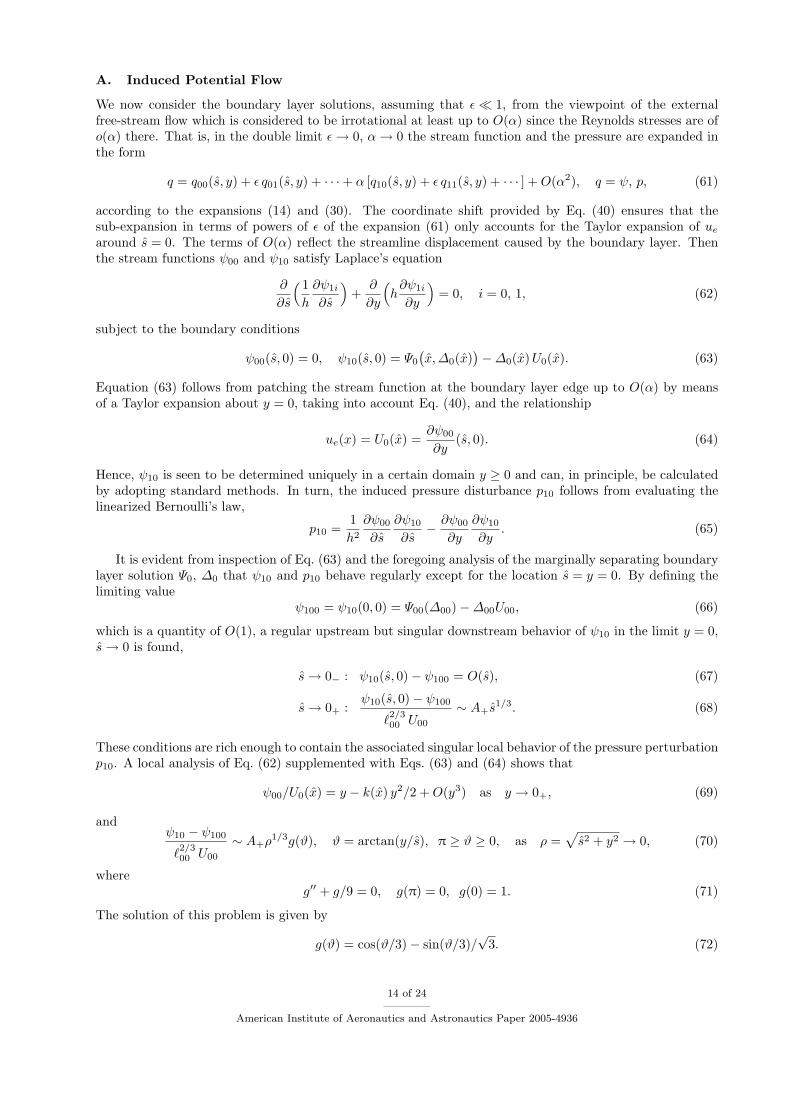
In the limit s→ 0 the stream function in the boundary layer where Y = O(1) is given by ψ ∼ αΨ00(Y ), seeEqs. (16) and (50). We now seek the perturbations there owing to the induced pressure p10 upstream anddownstream of s = 0. Inspection of the momentum equation (3) in combination with the near-wall behaviorgiven by Eq. (23) then shows that the disturbances caused by the pressure gradient ∂p10/∂s of both theReynolds shear and the inertia terms balance in, respectively, the regions I− and I+, see figure 3 on the nextpage, where the wall coordinate

η = Y/(ℓ2/300 |s|1/3) (76)

is a quantity of O(1). There, the following expansions are suggested in the triple limit ǫ→ 0, α→ 0, s→ 0both for

s→ 0− :ψ

ℓ2/300 P

1/200

= α[

(−s)5/6F−(η) + (−s)1/3(ǫ−Bs)η + (−s)4/3 B

180η4 + · · ·

]

+α2(−s)−5/6 ℓ2/300 U

200

P00G−(η) + · · · ,

p− p0(x0)

P00= s+ · · · − α (−s)−2/3 2A+

3√

3

ℓ2/300 U

200

P00+ · · · , (77)

and for

s→ 0+ :ψ

ℓ2/300 P

1/200

= α s5/6F+(η) + · · · + α2s−5/6 ℓ2/300 U

200

P00G+(η) + · · · ,

p− p0(x0)

P00= s+ · · · + α s−2/3 A+

3√

3

ℓ2/300 U

200

P00+ · · · . (78)

In the expansions (77) and (78) the exponentially growing terms considered in § III.C, which cause a break-down when s = O(ǫ2), are represented by dots. This is sufficient as we now rather focus on the perturbationsproportional to α which are responsible for the onset of the interaction process of the flow upstream anddownstream of the interaction region, cf. figure 3 on the following page.

15 of 24


IW

OW

II− I+

IIII− II+

III

s

y

∼ σ

∼ σ

∼ ασ1/3

∼ α3/2

y = δ(x) = O(α)

Figure 3. Asymptotic splitting of the flow due to the interaction process of the oncoming (subscripts −) anddownstream evolving (subscripts +) boundary layer (outer wake OW, inner wake IW, see § II.B.2), triple-deckstructure (lower deck I, main deck II, upper deck III).

Inserting expansions (77) and (78) into Eq. (3) and rearranging terms up to O(α|s|−5/3) gives rise to alinear inhomogeneous third-order problem for G∓(η),

±2(F ′′∓G

′′∓)′ − 5

6F∓G

′′∓ − 2

3F ′∓G

′∓ +

5

6F ′′∓G∓ = (−1 ∓ 3)

A+

9√

3, G∓(0) = G′′

∓(0) = 0, (79)

where the upper and the lower signs correspond to the upstream and the downstream case, respectively.

1. Upstream Onset of the Interaction Process

In the upstream case the problem (79) assumes the form

(η1/2G′′−)′ − 1

9η5/2G′′

− − 2

9η3/2G′

− +5

12η1/2G− = −2A+

9√

3, G−(0) = G′′

−(0) = 0. (80)

By applying the transformation

G−(η) = F ′−(η)

[∫ η

0

H(z) −H(0)

ζ3/2dζ − 2

H(0)

η1/2

]

, z =ζ3

27, (81)

Eq. (80) is conveniently cast into an inhomogeneous Kummer’s equation28 for H(z),

zH ′′ + (4/3 − z)H ′ − 7/6H = −A+/9 z−1/2 (82)

where the boundary conditions in Eq. (80) require H to be bounded for z → 0. In addition, the thirdboundary condition for G− missing in Eq. (80) follows from the requirement that H clearly must not growexponentially for z → ∞. The solution of (82) is found in terms of a hypergeometric series which, by usingthe integral representation of the Beta function,28 can be expressed in closed form as an integral. After somemanipulations we obtain

H(z) =A+

9

π

22/3 Γ(1/6) Γ(4/3)

∫ 1

0

t1/6 ezt erfc(√zt)

(1 − t)5/6dt. (83)

Inserting Eq. (83) into Eq. (81) then yields the limiting behavior of G−(η),

G′−(0) = −A+

√π

3√

3(84)

andG− = A−F

′−(η)[1 +O(η−2)] as η → ∞, (85)

16 of 24


where

A− =

∫ ∞

0

H(z) −H(0)

33/2 z7/6dz = −A+

27/3 Γ(5/6)√

π

27. (86)

We now consider the effect of the induced pressure on the surface slip velocity us which is defined by

us = ∂ψ/∂y at y = 0. (87)

For distances s = O(1), the surface slip is primarily given by the boundary layer solution, i.e.

us = Us(x) + · · · . (88)

Here the dots denote higher order terms due to finite values of ǫ and α. In the triple limit α→ 0, ǫ→ 0,s→ 0− evaluation of Eq. (77) gives

us

P1/200

= ǫ−Bs+ · · · + α(−s)−7/3 ℓ2/300 U

200

P00G′

−(0) + · · · , (89)

where the first terms on the right-hand side represent the expansion of Us(x) about x = x0, using Eq. (40).Equation (89) allows for an appealing physical interpretation: as indicated by Eqs. (77) and (84), thenegative (favorable) induced pressure gradient upstream of s = 0 causes a deceleration of the flow close tothe surface. This rather surprising phenomenon has not been observed yet in laminar boundary layer flows.Here, however, it originates from the fact that convection does not vanish at the surface.

Finally, matching of the expansions (77) and (78) with the flow in the boundary layer main regimes II−and II+ (figure 3 on the previous page) where Y = O(1) demonstrates, by noticing Eq. (85), that theexpansions of the stream function there take on the form

s→ 0− : ψ = α [Ψ00(Y ) + (ǫ−Bs)Ψ01(Y ) + · · · ] + α2(−s)−4/3 ℓ4/300 U

200

P00A− Ψ

′00(Y ) + · · · , (90)

s→ 0+ : ψ = α [Ψ00(Y ) + s1/3 ℓ2/300 A+Ψ

′00(Y ) + · · · ] + α2s−4/3 ℓ

4/300 U

200

P00C+ Ψ

′00(Y ) + · · · . (91)

It is anticipated in Eq. (91) that, in analogy to Eq. (85), the functionG+ behaves as G+(η) ∼ C+F′+(η +A+),

η → ∞, with some constant C+.21

2. Main Deck

A breakdown of the asymptotic structure considered so far occurs due to both the exponentially growingeigensolutions when s = O(ǫ2), see the expansion (30) and Eq. (40), and the singular induced pressuregradient ∂p10/∂s when s = O(α3/5), cf. the expansions (90) and (91) above. To take into account bothcauses of non-uniformness, we consider a distinguished limit by introducing the coupling parameter

χ =ǫ10/3

α

P00

ℓ2/300 U

200

, (92)

which is required to be of O(1) in the double limit ǫ→ 0, α→ 0. Then the streamwise distance where theexpansions (90), and (91) cease to be valid is found to be measured by

s = σX, σ = (ǫ/Γ )2 with 0 ≤ Γ ≤ 1, (93)

which in turn redefines the streamwise extent of the main deck (region II in figure 3 on the preceding page).Here the parameter Γ is introduced to provide a bijective function χ(Γ ) having the properties

χ′(Γ ) > 0, χb = χ(1) ≤ ∞, χ = O(Γ 10/3) as Γ → 0, (94)

where the upper bound χb of the coupling parameter may be chosen arbitrarily. It is convenient with respectto the subsequent analysis to specify the relationship between Γ and χ by the definition of a further functionΛ(Γ ) in the form

χ(Γ ) = Γ 10/3/Λ(Γ ), Λ′(Γ ) ≤ 0. (95)

17 of 24


Then Λ is seen to be bounded, andΛ(0) > Λ(1) = 1/χb. (96)

From Eqs. (92), (93) and (95) one then readily concludes that

ǫ = σ1/2Γ, α = σ5/3ΛP00

ℓ2/300 U

200

. (97)

The meaning of Eqs. (92)–(97) is the following: The case χb = ∞ or, equivalently, Λ(1) = 0, recoversthe pure boundary layer limit, that is α = 0 for finite values of ǫ, already discussed in § III.C.2, where theinduced pressure gradient does not come into play at all. On the other hand, the limit χ = 0 refers to thecase γ = ǫ = 0 where σ = O(α3/5). These considerations imply that the regions I, II, and III, as sketchedin figure 3 on page 16, are located a distance of O(ǫ) upstream of the position of the marginal singularitygiven by s = 0, cf. Eq. (40), where the lower and upper limits of the magnitude of their streamwise extentare given by O(α3/5) and O(ǫ2), respectively.

Inspection of Eqs. (90) and (91) indicates that, in the main-deck region, the expansions (50) and (51)now take on the asymptotically correct forms

ψ/α = Ψ00(Y ) + σ1/3 ℓ2/300 A(X)Ψ ′

00(Y ) + · · · + (σ1/2Γ − σBX)Ψ01(Y ) + · · · (98)

andδ/α = ∆00 − σ1/3 ℓ

2/300 A(X) + · · · (99)

in the limit σ → 0. Here and in the following the substitutions given by Eq. (97) have been applied. Moreover,the expansions (77) and (78) imply that the pressure in the main deck can be written as

p = p0(x0) + σP00[X + Λ P (X)] + · · · . (100)

Both the displacement function A(X) and the pressure function P (X) are quantities of O(1) and unknown atthis stage of the analysis. However, matching with the regions II− and II+ reveals the following asymptotes,

X → −∞ : A(X) ∼ ΛA− X−4/3, (101)

P (X) ∼ −2A+

3√

3X−2/3, (102)

X → +∞ : A(X) ∼ A+ X1/3, (103)

P (X) ∼ A+

3√

3X−2/3. (104)

3. Upper Deck

The above considerations suggest that the expansion (61) of the flow in the external regime where s and yare quantities of O(1) fail in the upper deck (region III in figure 3 on page 16). There appropriately rescaledvariables are given by the scalings (93) and

y = σy, y = O(1). (105)

The singular behavior of the stream function and the pressure expressed by Eqs. (68), (74), and (75) thengives rise to the expansions

ψ = σU00y + · · · + ΛP00

U00

[

σ5/3 Ψ100

ℓ2/300 U00

+ σ2ψ(X, y) + · · ·]

, (106)

p = p0(x0) + σP00[X + Λ p(X, y)] + · · · . (107)

Here terms proportional to Λ represent the potential flow induced locally by the boundary layer displacement.The pressure p is calculated from Bernoulli’s law, cf. Eq. (65), which by balancing terms up to O(σ2)

reduces to

p = −∂ψ∂y

, (108)

18 of 24


and the stream function ψ is seen to satisfy the Cauchy problem

∂2ψ

∂X2+∂2ψ

∂y2= 0, ψ(X, 0) = A(X), ψ ∼ A+ρ

1/3g(ϑ) as ρ =

√

X2 + y2 → ∞. (109)

Herein ϑ is given by Eq. (70) where the ratio y/s is to be replaced by y/X according to the local scalingprovided by Eqs. (105) and (93). The boundary conditions in Eq. (109) follow from patching the streamfunction at the boundary layer edge by using Eqs. (98), (99) and from a match with the singular behaviorof ψ10 given by Eq. (70), respectively. Additionally, comparing Eq. (107) with Eq. (100) and taking intoaccount Eq. (108) yields the relationship

∂ψ

∂y(X, 0) = −P (X) (110)

where P (X) is seen to be the induced surface pressure. Consequently, and as a well-known result frompotential theory,25 P (X) and −A′(X) form a Hilbert pair, i.e.

P (X), −A′(X) =1

π

∫ ∞

−∞

C A′(S), P (S)X − S

dS. (111)

4. Lower Deck

The analysis is finalized by considering the flow in the lower deck (region I in figure 3 on page 16) in thelimit σ → 0. Hence, we introduce rescaled local variables Y , Ψ of O(1) according to

Y

ℓ2/300

= σ1/3Y ,ψ

ℓ2/300 P

1/200

∼ ασ5/6 Ψ(X, Y ). (112)

Moreover, the pressure is given by Eq. (100). The leading-order problem governing the flow in the lower deckis found by inserting these quantities into the equations of motion (3) and (4) or, equivalently, by applyingthe transformation

X = Γ 2X, Y = Γ 2/3Y , Ψ = Γ 5/3Ψ (113)

to Eq. (42). As a result, the inclusion of the induced pressure gradient in Eq. (43) is seen to be sufficient togenerate an asymptotically correct description of the flow near the surface. The lower-deck equations thenread

∂Ψ

∂Y

∂2Ψ

∂Y ∂X− ∂Ψ

∂X

∂2Ψ

∂Y 2= −1 − Λ(Γ ) P ′(X) +

∂T

∂Y, T =

∂2Ψ

∂Y 2

∣

∣

∣

∣

∂2Ψ

∂Y 2

∣

∣

∣

∣

. (114)

They are subject to the boundary conditions

Y = 0 : Ψ = T = 0, (115)

Y → ∞ : T − Y → A(X), (116)

X → −∞ : Ψ → F−(Y ) + Γ Y , 0 ≤ Γ ≤ 1, (117)

X → ∞, Y → ∞ : Ψ X−5/6 → F+(η), η = Y /X1/3 = O(1). (118)

The conditions (117), (118), and (116) follow from a match with the expansions (77), (78), and (98), re-spectively, which clearly cease to be valid in the lower-deck flow regime. Most important, since both thefunctions P (X) and A(X) are seen to be part of the solution, Eqs. (114)–(118) have to be supplementedwith one of the relationships given by Eq. (111) in order to complete the triple-deck problem.

This fundamental problem which governs turbulent marginal separation associated with the triple-deckscheme outlined above has the following important properties:

(i) As a highly remarkable characteristic not known in laminar triple-deck theory at present, the lower-deck equations (114) include both the (locally constant) imposed and the induced streamwise pressuregradient given by ΛP ′(X).

19 of 24


(ii) A property also not observed in subsonic laminar interacting boundary layers so far is that turbulentmarginal separation is linked to the existence of eigensolutions of the underlying triple-deck prob-lem. In this connection we note that Eqs. (114)–(118) and Eq. (111) allow for the “trivial” solutionΨ = F−(Y ) + Γ Y , A(X) = P (X) = 0. However, a non-trivial solution is conveniently enforced by pre-scribing the downstream condition (118). Therefore, the ellipticity of the triple-deck problem is notonly due to the imposed pressure gradient, cf. Eq. (111), but also arises from the non-trivial downstreamstate as expressed by Eq. (118) and in agreement with Eq. (52).

(iii) It is inferred from Eq. (95) that the triple-deck solutions depend on χ solely, independent of the specificchoice of the function Λ(Γ ). This is also expressed by the invariance properties

Ψ(X, Y ) = λ−5/6 Ψ(X ,Y), A(X) = λ−1/3A(X ), P (X) = λ2/3P (X ),

X = λ(X − µ), Y = λ1/3 Y , (119)

satisfied by the solution Ψ , A, P for a given value of χ. Here X is stretched by an arbitrary factor λ > 0.The real parameter µ corresponds to an origin shift in X of the solution. However, the ambiguity of thesolution expressed by that translation invariance has to be eliminated by the exponentially decreasingeigensolutions occurring upstream, giving

Ψ = F−(Y ) + Γ Y + · · · − sgn(γ)Γ 5/3f(Y /Γ 2/3) exp(

X/(3Γ 2))

+ · · · , X → −∞. (120)

This expansion follows directly from Eq. (46) by taking into account Eq. (113). Equation (120) statesthat, in definite contrast to the non-interactive case which is expressed by Γ = 1 and Λ = 0 or, equiv-alently, Eq. (43), the interaction process is insensitive to the sign of γ. The latter rather enters thetriple-deck solution only via exponentially small terms. Their strength is fixed by the requirement of amatch with the oncoming flow, which in turn eliminates the translation invariance of the solution bymeans of an adequate choice of the group parameter µ.

It is useful to introduce the rescaled surface slip velocity

Us =∂Ψ

∂Y(X, 0). (121)

A comparison with Eq. (89) gives

us ∼ σ1/2P1/200 Us as X = O(1), (122)

and by matching of Eq. (121) with Eq. (77) or, equivalently, Eq. (89), and Eq. (78) one recovers the expansionsholding upstream and downstream, respectively,

X → −∞ : Us ∼ Γ − ΛG′−(0) X−7/6, (123)

X → +∞ : Us ∼ U+ X1/2. (124)

The latter of these relationships reflects the match with the non-trivial self-similar solution expressed byF+(η). The asymptotic behavior (123) is seen to be valid for all admissible values of Γ an Λ and demonstratesthe effect of both the exponentially decaying eigensolutions and of the induced pressure gradient on the triple-deck solution: The first determines the magnitude of the control parameter ǫ and, in turn, Γ , which fixesthe upstream limit of the surface slip. The upstream deceleration of the flow, however, is primarily causedby the induced pressure gradient the strength of which is measured by Λ.

C. Numerical Results

For the numerical treatment of the triple-deck problem posed by Eqs. (114)–(118) and Eq. (111) a carefullydevised variable transform which maps the interval −∞ < X <∞ onto the range [−1, 1] was performedin order to handle the singular upstream and downstream behavior at infinity in an efficient manner. Inaddition, also a coordinate stretching in Y -direction was introduced which, among others, regularizes thehalf-power behavior Ψ = Us(X) Y +O(Y 5/2) for Y → 0 and thus allows for a higher resolution of the flowclose to the surface. These ideas were put forward in its original form by Smith and Merkin,29 see also

20 of 24


Ref. 30 and Ref. 31. The thereby transformed equations were discretized on a uniformly spaced mesh byapproximating all derivatives using central finite-differences with second-order accuracy. Therefore, theelliptic character of the problem is fully retained. The resulting system of nonlinear algebraic equations wassolved directly by adopting a modification of the Powell hybrid method32 where the Jacobians are calculatednumerically. Under reasonable conditions this algorithm guarantees a fast rate of global convergence. Wenote that typically a grid of 110 points in X-direction and 60 points in Y -direction was employed wherethe principal limit of resolution depends on the hardware memory available. It should be stressed that theindeterminacy of the solutions with respect to a shift of the origin, expressed by Eq. (119) and discussedin (iii) above, is eliminated numerically as a consequence of the discretization process. A more detaileddescription of the numerical procedure, however, is postponed.21

Numerical solutions have been obtained for a various values of Λ whereas Γ varied in the whole range0 ≤ Γ ≤ 1. Owing to the limitation of space, only the case Λ = 3 will be discussed in detail. It then followsfrom Eq. (95) that χ = Γ 10/3/3 and 0 ≤ χ ≤ χb with χb = 1/3. Separation is associated with negative valuesof Us. As an important result, such local flow reversal is observed for 0 ≤ Γ ≤ Γ ∗ where Γ ∗ .

= 0.205, thatmeans within the (rather small) range 0 ≤ χ ≤ χ∗ with χ∗ .

= 1.69 × 10−3. We furthermore emphasize thatthe shear stress gradient at the surface, given by (∂T /∂Y )(X, 0), and, in turn, both the Reynolds stress Tand the streamwise velocity gradient ∂2Ψ/∂Y 2 are seen to be positive for all admissible values of X, Y , andχ.

Representative numerical results are plotted in figure 4, where consecutive data points are connected

−6.408

−6.409

0 0.004 0.008 0.012 0.016

−200

200

100

0

−100

Γ

XD

XR

L,

(a)

−20

−10

0

10

0.017 0.06 0.1 0.14 0.18 0.205

−6

−8

−7

−9Γ

XD XR

L,

(b)

0.017 0.0174 0.0178 0.0182 0.0186 0.019

7

3

5

1 −28

−26

−24

−22

−20

Γ

XD

XR,

L

(c)

4

3

2

1

0

−24 −20 −16 −12 −8 −4 4 8 12

40302010−10−20−30−40

−0.35

−0.2

−0.1

0

XD XR

A

A,

P

P

Us

Us

X

X

(d)

Figure 4. (a)–(c) Locations of detachment X = XD, reattachment X = XR, and bubble length L = XR − XD

in dependence of Γ where (c) applies to the first-separating flow regime, (d) solutions for Γ = 0.019. Here

XD

.= −18.01 and XR

.= −6.40. The abscissa at the bottom refers to A and Us, the one at the top to P .

21 of 24


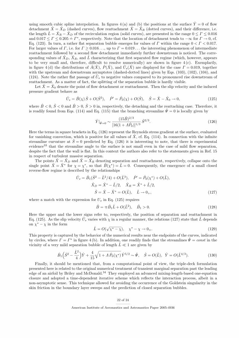
using smooth cubic spline interpolation. In figures 4 (a) and (b) the positions at the surface Y = 0 of flowdetachment X = XD (dashed curves), flow reattachment X = XR (dotted curves), and their difference, i.e.the length L = XR − XD of the recirculation region (solid curves), are presented in the range 0 ≤ Γ ≤ 0.016and 0.017 ≤ Γ ≤ 0.205

.= Γ ∗, respectively. Note that the location of detachment tends to −∞ for Γ → 0, cf.

Eq. (123). In turn, a rather flat separation bubble emerges for values of Γ within the range 0 < Γ < 0.017.For larger values of Γ , i.e. for Γ ≥ 0.016 . . ., up to Γ = 0.019 . . . the interesting phenomenon of intermediatereattachment followed by a second flow detachment immediately further downstream is noticed. The corre-sponding values of XD, XR, and L characterizing that first separated flow regime (which, however, appearsto be very small and, therefore, difficult to resolve numerically) are shown in figure 4 (c). Exemplarily,in figure 4 (d) the distributions of A(X), P (X), and Us(X) are displayed for the case Γ = 0.019, togetherwith the upstream and downstream asymptotes (dashed-dotted lines) given by Eqs. (103), (102), (104), and(124). Note the rather flat passage of Us to negative values compared to its pronounced rise downstream ofreattachment. As a matter of fact, the splitting of the separation bubble is hardly visible.

Let X = X0 denote the point of flow detachment or reattachment. Then the slip velocity and the inducedpressure gradient behave as

Us = B(χ) S +O(S2), P ′ = P0(χ) +O(S), S = X − X0 → 0, (125)

where B < 0, S < 0 and B > 0, S > 0 in, respectively, the detaching and the reattaching case. Therefore, itis readily found from Eqs. (114) and Eq. (115) that the branching streamline Ψ = 0 is locally given by

Y |Ψ=0 ∼ (15B)2/3

[16(1 + ΛP0)]1/3S2/3. (126)

Here the terms in square brackets in Eq. (126) represent the Reynolds stress gradient at the surface, evaluatedfor vanishing convection, which is positive for all values of X, cf. Eq. (114). In connection with the infinitestreamline curvature at S = 0 predicted by Eq. (126) it is interesting to note, that there is experimentalevidence33 that the streamline angle to the surface is not small even in the case of mild flow separation,despite the fact that the wall is flat. In this context the authors also refer to the statements given in Ref. 15in respect of turbulent massive separation.

The points X = XD and X = XR denoting separation and reattachment, respectively, collapse onto thesingle point X = X∗ for χ = χ∗, so that B(χ∗) = L = 0. Consequently, the emergence of a small closedreverse-flow regime is described by the relationships

Us = B1(S2 − L2/4) +O(L3), P ′ = P0(χ

∗) +O(L),

XD = X∗ − L/2, XR = X∗ + L/2,

S = X − X∗ = O(L), L→ 0+, (127)

where a match with the expression for Us in Eq. (125) requires

B = ∓B1L+O(L2), B1 > 0. (128)

Here the upper and the lower signs refer to, respectively, the position of separation and reattachment inEq. (125). As the slip velocity Us varies with χ in a regular manner, the relations (127) state that L dependson χ∗ − χ in the form

L = O(√χ∗ − χ), χ∗ − χ→ 0+. (129)

This property is captured by the behavior of the numerical results near the endpoints of the curves, indicatedby circles, where Γ = Γ ∗ in figure 4 (b). In addition, one readily finds that the streamlines Ψ = const in thevicinity of a very mild separation bubble of length L≪ 1 are given by

B1

(

S2 − L2

4

)

Y +4

15

√

1 + Λ P0(χ∗) Y 5/2 ∼ Ψ , S = O(L), Y = O(L4/3). (130)

Finally, it should be mentioned that, from a computational point of view, the triple-deck formulationpresented here is related to the original numerical treatment of transient marginal separation past the leadingedge of an airfoil by Briley and McDonald.34 They employed an advanced mixing-length-based one-equationclosure and adopted a time-dependent iterative scheme which reflects the interaction process, albeit in anon-asymptotic sense. This technique allowed for avoiding the occurrence of the Goldstein singularity in theskin friction in the boundary layer sweeps and the prediction of closed separation bubbles.

22 of 24


V. Conclusions and Further Outlook

An asymptotic theory of turbulent marginal separation has been presented which depends on a singlesimilarity parameter χ ≥ 0 containing the essential upstream information. Numerical solutions of the fun-damental triple-deck problem have been found for a wide range of χ. Open questions include, among others,the effect of the exponentially decaying eigensolutions as X → −∞ which dominate over the algebraicallyvarying terms for Γ = 1 in the non-interactive case Λ→ 0 or, equivalently, χ→ ∞ as predicted by Eq. (123).Then only the strictly attached solutions have been found at present, which are related to the sub-criticalupstream condition γ < 0. Its super-critical counterpart γ > 0, however, causing the boundary layer solutionto terminate in the Goldstein-type singularity, is likely associated with a very large recirculation region if theinduced pressure is taken into account in an appropriate manner. That is, the triple-deck problem has to beinvestigated in order to explore the according sub-structure emerging for Λ→ 0 and predicting separationon a correspondingly larger streamwise length scale.

Furthermore, the effects of the inner wake as well as the Reynolds-number-dependent flow regimes ad-jacent to the surface have to be studied. However, the inner wake layer, not considered here, is seen tobehave only passively as it is characterized by convective terms linearized about the slip velocity imposedby the outer wake. Most important, matching of the u-component of the velocity in the viscosity-affectedflow regimes gives rise to a relationship determining the surface friction τ in the limit Re → ∞,

√τ

us∼ κ

lnRe, τ =

1

Re

∂u

∂yat y = 0. (131)

That skin friction law is clearly rendered invalid if the surface slip us at the base of the wake tends to zerowhich is the case as separation is approached. Therefore, the investigation of a flow on the verge of separationwhere the reverse-flow regime is governed by Eq. (130) is expected to give a first hint how to continue theskin friction law (131) asymptotically correctly into the regions where the flow separates but immediatelyrecovers. Since the flow inside the viscous wall layer then plays a fundamental role in order to predict thesurface friction, a study of the time-dependent motions in that region is presumably necessary. The basisfor such a research is provided by the extensive work of Walker,8 Walker and Herzog,9 and Brinckman andWalker,10 see also Ref. 1, which, however, applies to a firmly attached turbulent boundary layer.

With respect to those aspects, which are presently under investigation, we add that results obtainedby means of Direct Numerical Simulation (DNS)35 indicate that small changes in the pressure distributiondue to an external flow which triggers the occurrence of a mild separation bubble have a relatively greatimpact on the skin friction distribution. Here we stress that this observation is corroborated by the theorypresented as the slip velocity is related to the skin friction through Eq. (131). A qualitative comparisonof the theory outlined here with the DNS study of marginal separation by Na and Moin36 as well as theLarge-Eddy Simulation by Cabot37 for the identical flow configuration is a topic of current research also.Unfortunately, a validation of the theoretical results with experimental data, although highly desirable,appears to be impossible on the basis of the existing material.

Acknowledgments

This work was supported by the Austrian Science Fund (FWF) under Grant No. P16555-N12.

References

1Walker, J. D. A., “Turbulent Boundary Layers II: Further Developments,” Recent Advances in Boundary Layer Theory,edited by A. Kluwick, Vol. 390 of CISM Courses and Lectures, Springer-Verlag, Vienna, New York, 1998, pp. 145–230.

2Degani, A. T., Smith, F. T., and Walker, J. D. A., “The Structure of a Three-Dimensional Turbulent Boundary Layer,”J. Fluid Mech., Vol. 250, 1993, pp. 43–68.

3Degani, A. T., Smith, F. T., and Walker, J. D. A., “The Three-Dimensional Turbulent Boundary Layer near a Plane ofSymmetry,” J. Fluid Mech., Vol. 234, 1992, pp. 329–360.

4Schlichting, H. and Gersten, K., Boundary-Layer Theory, Springer-Verlag, Berlin, Heidelberg, Germany, 8th ed., 2000.5Gersten, K., “Turbulent Boundary Layers I: Fundamentals,” Recent Advances in Boundary Layer Theory, edited by

A. Kluwick, Vol. 390 of CISM Courses and Lectures, Springer-Verlag, Vienna, New York, 1998, pp. 107–144.6Scheichl, B. F., Asymptotic Theory of Marginal Turbulent Separation, Ph.D. thesis, Vienna University of Technology,

Vienna, Austria, June 2001.

23 of 24


7Scheichl, B. and Kluwick, A., “Non-unique Turbulent Boundary Layer Flows Having a Moderately Large Velocity Defect:A Rational Extension of the Classical Asymptotic Theory,” Theoret. Comput. Fluid Dyn., 2005, submitted for publication.

8Walker, J. D. A., Abbott, D. E., Scharnhorst, R. K., and Weigand, G. G., “Wall-Layer Model for the Velocity Profile inTurbulent Flows,” AIAA J., Vol. 27, No. 2, 1989, pp. 140–149.

9Walker, J. D. A. and Herzog, S., “Eruption Mechanisms for Turbulent Flows near Walls,” Transport Phenomena inTurbulent Flows: Theory, Experiment, and Numerical Simulation. Proc. 2nd Intl Symp. Transport Phenomena in TurbulentFlows, Tokyo, October 1987 , edited by M. Hirata and N. Kasagi, Hemisphere Publishing Corp., New York, Washington,Philadelphia, London, 1988, pp. 145–156.

10Brinckman, K. W. and Walker, J. D. A., “Instability in a Viscous Flow Driven by Streamwise Vortices,” J. Fluid Mech.,Vol. 432, 2001, pp. 127–166.

11Ruban, A. I., “Singular Solutions of the Boundary Layer Equations Which Can Be Extended Continuously Through thePoint of Zero Surface Friction,” Fluid Dyn., Vol. 16, No. 6, 1981, pp. 835–843, original Russian article in Izv. Akad. Nauk SSSR,Mekh. Zhidk. i Gaza, No. 6, 1981, pp. 42–52.

12Ruban, A. I., “Asymptotic Theory of Short Separation Regions on the Leading Edge of a Slender Airfoil,” Fluid Dyn.,Vol. 17, No. 1, 1982, pp. 33–41, original Russian article in Izv. Akad. Nauk SSSR, Mekh. Zhidk. i Gaza, No. 1, 1982, pp. 42–51.

13Stewartson, K., Smith, F. T., and Kaups, K., “Marginal Separation,” Studies in Appl. Math., Vol. 67, No. 1, 1982,pp. 45–61.

14Sychev, V. V., Ruban, A. I., Sychev, Vic. V., and Korolev, G. L., Asymptotic Theory of Separated Flows, CambridgeUniversity Press, Cambridge, UK, 1998.

15Neish, A. and Smith, F. T., “On Turbulent Separation in the Flow past a Bluff Body,” J. Fluid Mech., Vol. 241, 1992,pp. 443–467.

16Melnik, R. E., “A New Asymptotic Theory of Turbulent Boundary Layers and the Turbulent Goldstein Problem,”Boundary-Layer Separation. Proc. IUTAM Symp., London, August 26–28, 1986 , edited by F. T. Smith and S. N. Brown,Springer-Verlag, New York, Berlin, Heidelberg, Germany, 1987, pp. 217–234.

17Melnik, R. E., “An Asymptotic Theory of Turbulent Separation,” Computers & Fluids, Vol. 17, No. 1, 1989, pp. 165–184.18Goldstein, S., “On Laminar Boundary Layer Flow near a Position of Separation,” Quart. J. Mech. Appl. Math., Vol. 1,

No. 1, 1948, pp. 43–69.19Stewartson, K., “Is the Singularity at Separation Removable?” J. Fluid Mech., Vol. 44, No. 2, 1970, pp. 347–364.20Scheichl, B. and Kluwick, A., “Singular Solutions of the Turbulent Boundary Layer Equations in the Case of Marginal

Separation as Re → ∞,” Advances in Turbulence IX. Proc. Ninth European Turbulence Conf., Southampton, U.K., July 2–5,2002 , edited by I. P. Castro, P. E. Hancock, and T. G. Thomas, International Center for Numerical Methods in Engineering(CIMNE), Barcelona, 2002, pp. 829–832.

21Scheichl, B. and Kluwick, A., “Turbulent Marginal Separation and the Turbulent Goldstein Problem,” AIAA J., 2006,in preparation.

22Schneider, W., “Boundary-Layer Theory of Free Turbulent Shear Flows,” Z. Flugwiss. Weltraumforsch. (J. Flight Sci.Space Research), Vol. 15, No. 3, 1991, pp. 143–158.

23Klebanoff, P. B., “Characteristics of Turbulence in a Boundary Layer with Zero Pressure Gradient,” NACATech. Rept. 1247, NASA Langley Research Center, Hampton, VA, 1955, also NACA Tech. Note 3178, 1954.

24Skare, P. E. and Krogstadt, P.-A., “A Turbulent Equilibrium Boundary Layer near Separation,” J. Fluid Mech., Vol. 272,1994, pp. 319–348.

25Rothmayer, A. P. and Smith, F. T., “Part III: High Reynolds Number Asymptotic Theories,” The Handbook of FluidDynamics, edited by R. W. Johnson, CRC Press, Boca Raton, FL (also Springer-Verlag, Heidelberg, Germany), 1998, pp.III.1–25.26.

26Messiter, A. F., “Boundary-Layer Flow near the Trailing Edge of a Flat Plate,” SIAM J. Appl. Math., Vol. 18, No. 1,1970, pp. 241–257.

27Stewartson, K., “On the Flow near the Trailing Edge of a Flat Plate II,” Mathematika, Vol. 16, No. 1, 1969, pp. 106–121.28Abramowitz, M. and Stegun, I. A., Handbook of Mathematical Functions, Dover Publications, New York, 9th ed., 1972.29Smith, F. T. and Merkin, J. H., “Triple-Deck Solutions for Subsonic Flows past Humps, Steps, Concave or Convex

Corners and Wedged Trailing Edges,” Computers & Fluids, Vol. 10, No. 1, 1982, pp. 7–25.30Cassel, K. W., Ruban, A. I., and Walker, J. D. A., “An Instability in Supersonic Boundary-Layer Flow over a Compression

Ramp,” J. Fluid Mech., Vol. 300, 1995, pp. 265–285.31Gajjar, J. S. B. and Turkyılmazoglu, M., “On the Absolute Instability of the Triple-Deck Flow over Humps and near

Wedged Trailing Edges,” Phil. Trans. R. Soc. Lond. A, Vol. 358, No. 1777, 2000, pp. 3113–3128.32Powell, M. J. D., “A Hybrid Method for Nonlinear Algebraic Equations,” Numerical Methods for Nonlinear Algebraic

Equations, edited by P. Rabinowitz, Gordon and Breach, London, 1970, pp. 87–114, Chap. 6.33Cutler, A. D. and Johnston, J. P., “Adverse Pressure Gradient and Separating Turbulent Boundary Flows: The Effect of

Disequilibrium in Initial Conditions,” Rept. MD-46, Thermosciences Div., Mech. Engng Dept., Stanford University, Stanford,CA, 1984.

34Briley, W. R. and McDonald, H., “Numerical Prediction of Incompressible Separation Bubbles,” J. Fluid Mech., Vol. 69,No. 4, 1975, pp. 631–656.

35Skote, M. and Henningson, D. S., “Direct Numerical Simulation of a Separated Turbulent Boundary Layer,” J. FluidMech., Vol. 471, 2002, pp. 107–136.

36Na, Y. and Moin, P., “Direct Numerical Simulation of a Separated Turbulent Boundary Layer,” J. Fluid Mech., Vol. 374,1998, pp. 379–405.

37Cabot, W., “Large-Eddy Simulation of a Separated Boundary Layer,” Annual Research Briefs 1998 , Center for Turbu-lence Research, NASA/Ames, Stanford University, Stanford, CA, 1998, pp. 279–287.

24 of 24


4th aiaa theoretical fluid mechanics meeting, 6–9 june ... · 4th aiaa theoretical fluid...

Documents