4F10: Deep Learning

Mark Gales

Michaelmas 2016

What is Deep Learning?

From Wikipedia:Deep learning is a branch of machine learning based on aset of algorithms that attempt to model high-levelabstractions in data by using multiple processing layers,with complex structures or otherwise, composed ofmultiple non-linear transformations.

2/68

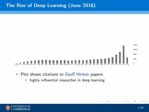
The Rise of Deep Learning (June 2016)

• Plot shows citations to Geoff Hinton papers• highly influential researcher in deep learning

3/68

Overview

• Basic Building Blocks• neural network architectures• activation functions

• Error Back Propagation• single-layer perceptron (motivation)• multiple-layer perceptron

• Optimisation• gradient descent refinement• second-order approaches, and use of curvature• initialisation

• Example• encoder-decoder models for sequence-to-sequence models• and attention for sequence-to-sequence modelling

4/68

Basic BuildingBlocks

5/68

Deep Neural Networks [12]

y(x)x

• General mapping process from input x to output y(x)

y(x) = F(x)

• deep refers to number of hidden layers• Output from the previous layer connected to following layer:

• x(k) is the input to layer k• x(k+1) = y(k) the output from layer k

6/68

Neural Network Layer/Node

φ()wi

zi

• General form for layer k:

y (k)i = φ(w ′

ix(k)+ bi) = φ(z(k)

i )

7/68

Initial Neural Network Design Options

• The input and outputs to the network are defined• able to select number of hidden layers• able to select number of nodes per hidden layer

• Increasing layers/nodes increases model parameters• need to consider how well the network generalises

• For fully connected networks, number of parameters (N) is

N = d ×N(1)+K ×N(L)

+L−1∑k=1

N(k)×N(k+1)

• L is the number of hidden layers• N(k) is the number of nodes for layer k• d is the input vector size, K is the output size

• Designing “good” networks is complicated ...

8/68

Activation Functions

• Heaviside (or step/threshold) function: output binary

φ(zi) = 0, zi < 01, zi ≥ 0

• Sigmoid function: output continuous, 0 ≤ yi(x) ≤ 1.

φ(zi) =1

1 + exp(−zi)

• Softmax function: output 0 ≤ yi(x) ≤ 1, ∑ni=1 yi(x) = 1.

φ(zi) =exp(zi)

∑nj=1 exp(zj)

• Hyperbolic tan function: output continuous, −1 ≤ yi(x) ≤ 1.

φ(zi) =exp(zi) − exp(−zi)

exp(zi) + exp(−zi)

9/68

Activation Functions

−5 −4 −3 −2 −1 0 1 2 3 4 5−1

−0.8

−0.6

−0.4

−0.2

0

0.2

0.4

0.6

0.8

1

• Activation functions:• step function (green)• sigmoid function (red)• tanh function (blue)

• softmax, usual output layer for classification tasks• sigmoid/tanh, often used for hidden layers

10/68

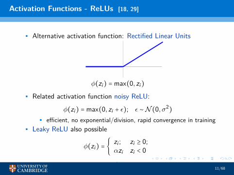
Activation Functions - ReLUs [18, 29]

• Alternative activation function: Rectified Linear Units

φ(zi) = max(0, zi)

• Related activation function noisy ReLU:

φ(zi) = max(0, zi + ε); ε ∼ N (0, σ2)• efficient, no exponential/division, rapid convergence in training

• Leaky ReLU also possible

φ(zi) = zi ; zi ≥ 0;αzi zi < 0

11/68

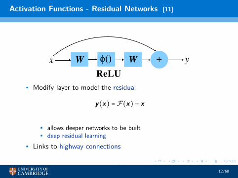
Activation Functions - Residual Networks [11]

φ()x y+

ReLU

W W

• Modify layer to model the residual

y(x) = F(x) + x

• allows deeper networks to be built• deep residual learning

• Links to highway connections

12/68

Pooling/Max-Out Functions [15, 26]

• Possible to pool the output of a set of node• reduces the number of weights to connect layers together

ϕ()

• A range of functions have been examined

• maxout φ(y1, y2, y3) = max(y1, y2, y3)• soft-maxout φ(y1, y2, y3) = log(∑3

i=1 exp(yi))• p-norm φ(y1, y2, y3) = (∑

3i=1 ∣yi ∣)

1/p

• Has also been applied for unsupervised adaptation

13/68

Convolutional Neural Networks [14, 1]

n frames

k fre

quencie

s

pooling layer

filter 1

filter n

14/68

Convolutional Neural Networks

• Various parameters control the form of the CNN:• number (depth): how many filters to use• receptive field (filter size): height/width/depth (h ×w × d)• stride: how far filter moves in the convolution• dilation: “gaps” between filter elements• zero-padding: do you pad the edges of the “image” with zeroes

• Filter output can be stacked to yield depth for next layer• To illustrate the impact consider 1-dimensional case - default:

• zero-padding, stride=1, dilation=0

sequence: 1,2,3,4,5,6 filter: 1,1,1

default: 3,6,9,12,15,11 no padding: 6,9,12,15dilation=1: 4,6,9,12,8,10 stride=2: 3,9,15

15/68

Convolutional Neural Network (cont)

• For a 2-dimensional image the convolution can be written as

φ(zij) = φ(∑kl

wklx(i−k)(j−l))

• xij is the image value at point i , j• wkl is the weight at point k, l• φ is the non-linear activation function

• For a 5 × 5 receptive field (no dilation)• k ∈ −2,−1,0,1,2• l ∈ −2,−1,0,1,2

• Stride determines how i and j vary as we move over the image

16/68

CNN Max-Pooling (Subsampling)

• Max-Pooling over a 2 × 2 filter on 4 × 4 “image”• stride of 2 - yields output of 2 × 2

• Possible to also operate with a stride of 1 overlapping pooling

17/68

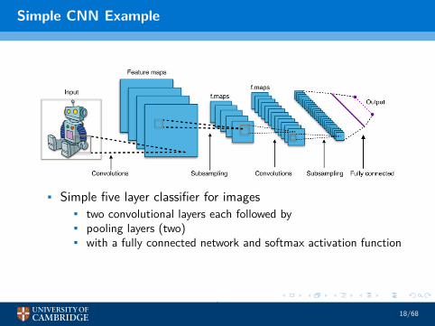
Simple CNN Example

• Simple five layer classifier for images• two convolutional layers each followed by• pooling layers (two)• with a fully connected network and softmax activation function

18/68

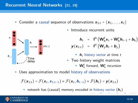
Recurrent Neural Networks [21, 19]

• Consider a causal sequence of observations x1∶t = x1, . . . ,xt

tx

t−1h

t

Time

h

delay

1:ty(x )

• Introduce recurrent units

ht = fh (Wfhxt +Wr

hht−1 + bh)

y(x1∶t) = ff (Wyht + by)

• ht history vector at time t• Two history weight matrices

• Wfh forward, Wr

h recursion• Uses approximation to model history of observations

F(x1∶t) = F(xt ,x1∶t−1) ≈ F(xt ,ht−1) ≈ F(ht) = y(x1∶t)

• network has (causal) memory encoded in history vector (ht)

19/68

RNN Variant: Bi-Directional RNN [23]

xt+1xt

ht t+1h

yt yt+1

t

ht

~

t+1h~

ht t+1h

yt yt+1

xt+1x

RNN Bi-Directional RNN

• Bi-directional: use complete observation sequence - non-causal

Ft(x1∶T ) = F(x1∶t ,xt ∶T ) ≈ F(ht , ht) = y t(x1∶T )

20/68

Latent Variable (Variational) RNN (reference) [7]

xt+1xt

ht t+1h

yt yt+1

t

ht t+1h

yt yt+1

z t z t+1

xt+1x

RNN Variational RNN

• Variational: introduce latent variable sequence z1∶T

p(y t ∣x1∶t) ≈ ∫ p(y t ∣xt , zt ,ht−1)p(zt ∣ht−1)dzt

≈ ∫ p(y t ∣ht)p(zt ∣ht−1)dzt• zt a function of complete history (complicates training)

21/68

Network Gating

• A flexible extension to activation function is gating• standard form is (σ() sigmoid activation function)

i = σ(Wfxt +Wrht−1 + b)

• vector acts a probabilistic gate on network values

• Gating can be applied at various levels• features: impact of input/output features on nodes• time: memory of the network• layer: influence of a layer’s activation function

22/68

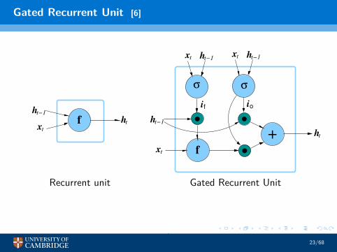
Gated Recurrent Unit [6]

xt

ht

h

ft−1

ht−1xt

if

ht

io

ht−1

σ σ

+

x

f

t ht−1

xt

Recurrent unit Gated Recurrent Unit

23/68

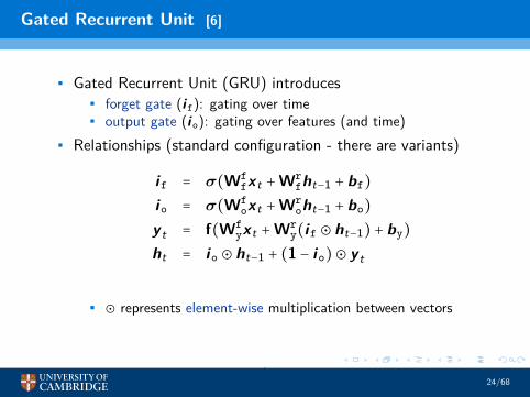
Gated Recurrent Unit [6]

• Gated Recurrent Unit (GRU) introduces• forget gate (if): gating over time• output gate (io): gating over features (and time)

• Relationships (standard configuration - there are variants)

if = σ(Wffxt +Wr

fht−1 + bf)

io = σ(Wfoxt +Wr

oht−1 + bo)

y t = f(Wfyxt +Wr

y(if ⊙ ht−1) + by)

ht = io ⊙ ht−1 + (1 − io)⊙ y t

• ⊙ represents element-wise multiplication between vectors

24/68

Long-Short Term Memory Networks (reference) [13, 10]

t

xt

ht−1

ht

xt ht−1

ct fh

fm

xt ht−1

σ σ

σ

i

time delay

f

iiio

ht−1x

25/68

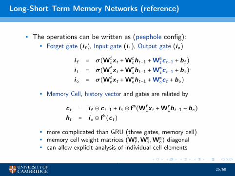
Long-Short Term Memory Networks (reference)

• The operations can be written as (peephole config):• Forget gate (if), Input gate (ii), Output gate (io)

if = σ(Wffxt +Wr

fht−1 +Wmfct−1 + bf)

ii = σ(Wfixt +Wr

iht−1 +Wmict−1 + bi)

io = σ(Wfoxt +Wr

oht−1 +Wmoct + bo)

• Memory Cell, history vector and gates are related by

ct = if ⊙ ct−1 + ii ⊙ fm(Wf

cxt +Wrcht−1 + bc)

ht = io ⊙ fh(ct)

• more complicated than GRU (three gates, memory cell)• memory cell weight matrices (Wm

f,Wmi,Wm

o) diagonal• can allow explicit analysis of individual cell elements

26/68

Highway Connections [25]

ht−1xt

ih

ht

xt

σ

+

h

ft−1

xt

• Gate the output of the node (example from recurrent unit)• combine with output from previous layer (xt)

ih = σ(Wflxt +Wr

lht−1 + bl)

ht = ih ⊙ f(Wfhxt +Wr

hht−1 + bh) + (1 − ih)⊙ xt

27/68

Example Deep Architecture: ASR (reference) [22]

understand the CLDNN architecture are presented in Section 4. Re-sults on the larger data sets are then discussed in Section 5. Finally,Section 6 concludes the paper and discusses future work.

2. MODEL ARCHITECTURE

This section describes the CLDNN architecture shown in Figure 1.

2.1. CLDNN

Frame xt, surrounded by l contextual vectors to the left and r con-textual vectors to the right, is passed as input to the network. Thisinput is denoted as [xtl, . . . , xt+r]. In our work, each frame xt isa 40-dimensional log-mel feature.

First, we reduce frequency variance in the input signal by pass-ing the input through a few convolutional layers. The architectureused for each CNN layer is similar to that proposed in [2]. Specif-ically, we use 2 convolutional layers, each with 256 feature maps.We use a 9x9 frequency-time filter for the first convolutional layer,followed by a 4x3 filter for the second convolutional layer, and thesefilters are shared across the entire time-frequency space. Our pool-ing strategy is to use non-overlapping max pooling, and pooling infrequency only is performed [11]. A pooling size of 3 was used forthe first layer, and no pooling was done in the second layer.

The dimension of the last layer of the CNN is large, due to thenumber of feature-mapstimefrequency context. Thus, we add alinear layer to reduce feature dimension, before passing this to theLSTM layer, as indicated in Figure 1. In [12] we found that addingthis linear layer after the CNN layers allows for a reduction in pa-rameters with no loss in accuracy. In our experiments, we found thatreducing the dimensionality, such that we have 256 outputs from thelinear layer, was appropriate.

After frequency modeling is performed, we next pass the CNNoutput to LSTM layers, which are appropriate for modeling the sig-nal in time. Following the strategy proposed in [3], we use 2 LSTMlayers, where each LSTM layer has 832 cells, and a 512 unit projec-tion layer for dimensionality reduction. Unless otherwise indicated,the LSTM is unrolled for 20 time steps for training with truncatedbackpropagation through time (BPTT). In addition, the output statelabel is delayed by 5 frames, as we have observed with DNNs thatinformation about future frames helps to better predict the currentframe. The input feature into the CNN has l contextual frames tothe left and r to the right, and the CNN output is then passed to theLSTM. In order to ensure that the LSTM does not see more than 5frames of future context, which would increase the decoding latency,we set r = 0 for CLDNNs.

Finally, after performing frequency and temporal modeling, wepass the output of the LSTM to a few fully connected DNN layers.As shown in [5], these higher layers are appropriate for producing ahigher-order feature representation that is more easily separable intothe different classes we want to discriminate. Each fully connectedlayer has 1,024 hidden units.

2.2. Multi-scale Additions

The CNN takes a long-term feature, seeing a context of tl to t (i.e.,r = 0 in the CLDNN), and produces a higher order representationof this to pass into the LSTM. The LSTM is then unrolled for 20timesteps, and thus consumes a larger context of 20 + l. However,we feel there is complementary information in also passing the short-term xt feature to the LSTM. In fact, the original LSTM work in[3] looked at modeling a sequence of 20 consecutive short-term xt

C

...

D

D

L

L

Cconvolutional

layers

LSTMlayers

fullyconnected

layers

output targets

[xt-l,..., xt, ...., xt+r]

linearlayer

dimred

(1)

xt

(2)

Fig. 1. CLDNN Architecture

features, with no context. In order to model short and long-termfeatures, we take the original xt and pass this as input, along withthe long-term feature from the CNN, into the LSTM. This is shownby dashed stream (1) in Figure 1.

The use of short and long-term features in a neural network hasbeen explored previously (i.e., [13, 14]). The main difference be-tween previous work and ours is that we are able to do this jointlyin one network, namely because of the power of the LSTM sequen-tial modeling. In addition, our combination of short and long-termfeatures results in a negligible increase in the number of networkparameters.

In addition, we explore if there is complementarity betweenmodeling the output of the CNN temporally with an LSTM, as wellas discriminatively with a DNN. Specifically, motivated by work incomputer vision [10], we explore passing the output of the CNN intoboth the LSTM and DNN. This is indicated by the dashed stream(2) in Figure 1. This idea of combining information from CNN andDNN layers has been explored before in speech [11, 15], thoughprevious work added extra DNN layers to do the combination. Ourwork differs in that we pass the output of the CNN directly into theDNN, without extra layers and thus minimal parameter increase.

• Example Architecture from Google (2015)• C: CNN layer (with pooling)• L: LSTM layer• D: fully connected layer

• Two multiple layer “skips”• (1) connects input to LSTM input• (2) connects CNN output to DNN input

• Additional linear projection layer• reduces dimensionality• and number of network parameters!

28/68

Network Training andError Back Propagation

29/68

Training Data: Classification

• Supervised training data comprises• x i : d-dimensional training observation• yi : class label, K possible (discrete) classes

• Encode class labels as 1-of-K (“one-hot”) coding: yi → t i• t i is the K -dimensional target vector for x i• zero other than element associated with class-label yi

• Consider a network with parameters θ and training examples:

x1, t1 . . . ,xn, tn

• need “distance” from target t i to network output y(x i)

30/68

Training Criteria

• Least squares error: one of the most common training criteria.

E(θ) =12

n∑p=1

∣∣y(xp) − tp)∣∣2=12

n∑p=1

K∑i=1

(yi(xp) − tpi)2

• Cross-Entropy: note non-zero minimum (entropy of targets)

E(θ) = −n∑p=1

K∑i=1

tpi log(yi(xp))

• Cross-Entropy for two classes: single binary target

E(θ) = −n∑p=1

(tp log(y(xp)) + (1 − tp) log(1 − y(xp)))

31/68

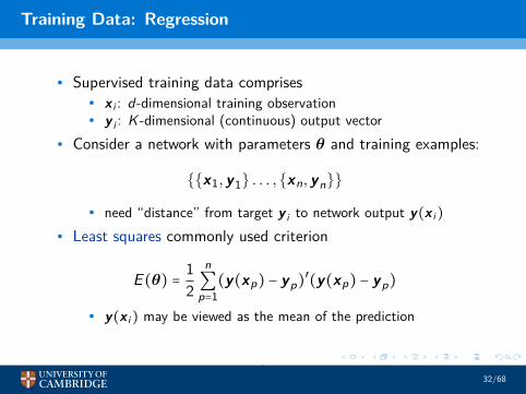
Training Data: Regression

• Supervised training data comprises• x i : d-dimensional training observation• y i : K -dimensional (continuous) output vector

• Consider a network with parameters θ and training examples:

x1,y1 . . . ,xn,yn

• need “distance” from target y i to network output y(x i)

• Least squares commonly used criterion

E(θ) =12

n∑p=1

(y(xp) − yp)′(y(xp) − yp)

• y(x i) may be viewed as the mean of the prediction

32/68

Maximum Likelihood - Regression Criterion

• Generalise least squares (LS) to maximum likelihood (ML)

E(θ) =n∑p=1

log(p(yp ∣xp,θ))

• LS is ML with a single Gaussian, identity covariance matrix• Criterion appropriate to deep learning for generative models• Output-layer activation function to ensure valid distribution

• consider the case of the variance σ > 0• apply an exponential activation function for variances

exp (yi(x)) > 0

• for means just use a linear activation function

33/68

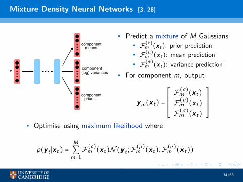
Mixture Density Neural Networks [3, 28]

componentmeans

component

component

(log) variances

priors

tx

• Predict a mixture of M Gaussians• F(c)

m (xt): prior prediction• F(µ)

m (xt): mean prediction• F(σ)

m (xt): variance prediction• For component m, output

ym(xt) =

⎡⎢⎢⎢⎢⎢⎢⎣

F(c)m (xt)

F(µ)m (xt)

F(σ)m (xt)

⎤⎥⎥⎥⎥⎥⎥⎦

• Optimise using maximum likelihood where

p(y t ∣xt) =M∑m=1F

(c)m (xt)N (y t ;F(µ)

m (xt),F(σ)m (xt))

34/68

Gradient Descent [20]

• If there is no closed-form solution - use gradient descent

θ[τ + 1] = θ[τ] −∆θ[τ] = θ[τ] − η ∂E∂θ

∣θ[τ]

• how to get the gradient for all model parameters• how to avoid local minima• need to consider how to set η

35/68

Network Training

• Networks usually have a large number of hidden layers (L)• enables network to model highly non-linear, complex, mappings• complicates the training process of the network parameters

• Network parameters are (usually) weights for each layer• merging bias vector for each layer into weight matrix

θ = W (1), . . . ,W (L+1)

Σ

wd

w2

w1

1

x

x

x

1

2

d

y(x)z

functionActivation

b

• Initially just consider a single layer perceptron

36/68

Single Layer Perceptron Training

• Take the example of least squares error cost function

E(θ) =12

n∑p=1

∣∣y(xp) − tp)∣∣2=

n∑p=1

E (p)(θ)

• Use chain rule to compute derivatives through network∂E(θ)

∂wi= (

∂E(θ)

∂y(x))(∂y(x)∂z

)(∂z∂wi

)

• change of error function with network output (cost function)• change of network output with z (activation function)• change of z with network weight (parameter to estimate)

• For a sigmoid activation function this yields

∂E (p)(θ)

∂wi= (y(xp) − tp)y(xp)(1 − y(xp))xpi

37/68

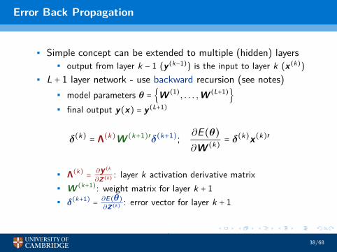
Error Back Propagation

• Simple concept can be extended to multiple (hidden) layers• output from layer k − 1 (y(k−1)) is the input to layer k (x(k))

• L + 1 layer network - use backward recursion (see notes)• model parameters θ = W (1), . . . ,W (L+1)

• final output y(x) = y(L+1)

δ(k)= Λ(k)W (k+1)′δ(k+1); ∂E(θ)

∂W (k) = δ(k)x(k)′

• Λ(k)=∂y (k∂z(k) : layer k activation derivative matrix

• W (k+1): weight matrix for layer k + 1• δ(k+1)

=∂E(θ)∂z(k) : error vector for layer k + 1

38/68

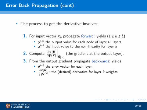
Error Back Propagation (cont)

• The process to get the derivative involves:

1. For input vector xp propagate forward: yields (1 ≤ k ≤ L)• y(k) the output value for each node of layer all layers• z(k) the input value to the non-linearity for layer k

2. Compute ∂E(θ∂y(x)

∣θ[τ]

(the gradient at the output layer).

3. From the output gradient propagate backwards: yields• δ(k) the error vector for each layer• ∂E(θ)

∂W (k) : the (desired) derivative for layer k weights

39/68

Optimisation

40/68

Batch/On-Line Gradient Descent

• The default gradient is computed over all samples• for large data sets very slow - each update

• Modify to batch update - just use a subset of data, D,

E(θ) = −∑p∈D

K∑i=1

tpi log(yi(xp))

• How to select the subset, D?• small subset “poor” estimate of true gradient• large subset each parameter update is expensive

• One extreme is to update after each sample• D comprises a single sample in order• “noisy” gradient estimate for updates

41/68

Stochastic Gradient Descent (SGD)

• Two modifications to the baseline approaches1. Randomise the order of the data presented for training

• important for structured data2. Introduce mini-batch updates

• D is a (random) subset of the training data• better estimate of the gradient at each update• but reduces number of iterations

• Mini-batch updates are (almost) always used• make use of parallel processing (GPUs) for efficiency

• Research of parallel versions of SGD on-going

42/68

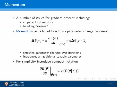
Momentum

• A number of issues for gradient descent including:• stops at local maxima• handling “ravines”

• Momentum aims to address this - parameter change becomes:

∆θ[τ] = η ∂E(θ)

∂θ∣θ[τ]

+ α∆θ[τ − 1]

• smooths parameter changes over iterations• introduces an additional tunable parameter

• For simplicity introduce compact notation

∂E(θ)

∂θ∣θ[τ]

= ∇(E(θ[τ]))

43/68

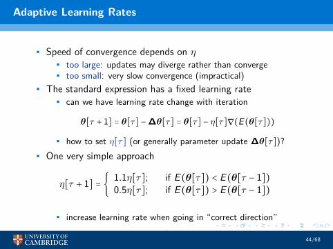
Adaptive Learning Rates

• Speed of convergence depends on η• too large: updates may diverge rather than converge• too small: very slow convergence (impractical)

• The standard expression has a fixed learning rate• can we have learning rate change with iteration

θ[τ + 1] = θ[τ] −∆θ[τ] = θ[τ] − η[τ]∇(E(θ[τ]))

• how to set η[τ] (or generally parameter update ∆θ[τ])?• One very simple approach

η[τ + 1] = 1.1η[τ]; if E(θ[τ]) < E(θ[τ − 1])0.5η[τ]; if E(θ[τ]) > E(θ[τ − 1])

• increase learning rate when going in “correct direction”

44/68

Gradient Descent Refinements (reference)

• Nesterov: concept of gradient at next iteration

∆θ[τ] = η∇(E(θ[τ] − α∆θ[τ − 1])) + α∆θ[τ − 1]

• AdaGrad: dimension specific learning rates (ε floor parameter)

∆θ[τ] = ηβt ⊙∂E(θ)

∂θ∣θ[τ]

; βti =1

√ε +∑τ

t=1∇i(E(θ[t]))2

• ε is a smoothing term to avoid division by zero• Adam: Adaptive Moment Estimation: use dimension moments

∆θi[τ] =η√

σ2τ i+ε

µτ i ; µτ i = α1µ(τ−1)i + (1 − α1)∇i(E(θ[τ]))

σ2τ i = α2σ2(τ−1)i + (1 − α2)∇i(E(θ[τ]))2

• additional normalisation applied to µτ i and σ2τ i to offsetinitialisation bias

45/68

Second-Order Approximations

• Gradient descent makes use of first-order derivatives of• what about higher order derivatives? Consider

E(θ) = E(θ[τ]) + (θ − θ[τ])′g + 12(θ − θ[τ])′H(θ − θ[τ]) +O(θ3)

where

g = ∇E(θ[τ]); (H)ij = hij =∂2E(θ)

∂θi∂θj∣θ[τ]

• Ignoring higher order terms and equating to zero

∇E(θ) = g +H(θ − θ[τ])

Equating to zero (check minimum!) - H−1g Newton direction

θ[τ + 1] = θ[τ] −H−1g; ∆θ[τ] = H−1g

46/68

Issues with Second-Order Approaches

1. The evaluation of the Hessian may be computationallyexpensive as O(N2) parameters must be accumulated foreach of the n training samples.

2. The Hessian must be inverted to find the direction, O(N3).This gets very expensive as N gets large.

3. The direction given need not head towards a minimum - itcould head towards a maximum or saddle point. This occurs ifthe Hessian is not positive-definite i.e.

v′Hv > 0

for all v. The Hessian may be made positive definite using

H = H + λI

If λ is large enough then H is positive definite.4. If the surface is highly non-quadratic the step sizes may be

too large and the optimisation becomes unstable.

47/68

QuickProp

• Interesting making use of the error curvature, assumptions:• error surface is quadratic in nature• weight gradients treated independently (diagonal Hessian)

• Using these assumptionsE(θ) ≈ E(θ[τ]) + b(θ − θ[τ]) + a(θ − θ[τ])2

∂E(θ)

∂θ≈ b + 2a(θ − θ[τ])

• To find a and b make use of:• update step, ∆θ[τ − 1], and gradient, g[τ − 1], iteration τ − 1• the gradient at iteration τ is g[τ]• after new update ∆θ[τ] the gradient should be zero

• The following equalities are obtainedg[τ − 1] = b − 2a∆θ[τ − 1], 0 = b + 2a∆θ[τ], g[τ] = b

→∆θ[τ] = g[τ]g[τ − 1] − g[τ]

∆θ[τ − 1]

48/68

QuickProp (cont)

0 0.2 0.4 0.6 0.8 1 1.2 1.4 1.6 1.8 24

4.5

5

5.5

6

6.5

7

θ[τ−1] θ[τ]

• The operation of quick-prop is illustrated above:• the assumed quadratic error surface is shown in blue• the statistics for quickprop are shown in red

• Parameter at minimum of quadratic approximation:θ[τ + 1] = 1

49/68

Regularisation

• A major issues with training networks is generalisation• Simplest approach is early stopping

• don’t wait for convergence - just stop ...• To address this forms of regularisation are used

• one standard form is (N is the total number of weights):

E(θ) = E(θ) + νΩ(θ); Ω(θ) =12

N∑i=1

w2i

• a zero "prior" is used for the model parameters• Simple to include in gradient-descent optimisation

∇E(θ[τ]) = ∇E(θ[τ]) + νw[τ]

50/68

Dropout [24]

Input

xd

y (x)1

y (x)k

Layer

Inputs

LayerOutput

Outputs

Hidden Layers

In−active node

Active node

x1

• Dropout is simple way of improving generalisation1. randomly de-activate (say) 50% of the nodes in the network2. update the model parameters

• Prevents a single node specialising to a task

51/68

Network Initialisation: Data Pre-Processing

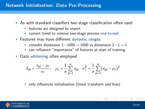
• As with standard classifiers two stage classification often used• features are designed by expert• current trend to remove two-stage process end-to-end

• Features may have different dynamic ranges• consider dimension 1:−1000→ 1000 vs dimension 2:−1→ 1• can influence “importance” of features at start of training

• Data whitening often employed

xpi =xpi − µi

σi; µi =

1n

n∑p=1

xpi σ2i =1n

n∑p=1

(xpi − µi)2

• only influences initialisation (linear transform and bias)

52/68

Network Initialisation: Weight Parameters

• A starting point (initialisation) for gradient descent is useful• one of the “old” concerns with deep networks was initialisation• recurrent neural networks are very deep!

• It is not possible to guarantee a good starting point, but• would like a parsimonious initialisation

• What about Gaussian random initialisation• consider zero mean distribution, scale the variance• sigmoid non-linearity

−10 −8 −6 −4 −2 0 2 4 6 8 100

0.1

0.2

0.3

0.4

0.5

0.6

0.7

0.8

0.9

1

Saturated SaturatedLinear

53/68

Gaussian Initialisation

0 0.1 0.2 0.3 0.4 0.5 0.6 0.7 0.8 0.9 10

20

40

60

80

100

120

140

160

180

200

0 0.1 0.2 0.3 0.4 0.5 0.6 0.7 0.8 0.9 10

20

40

60

80

100

120

140

160

N (0,1) N (0,2)

0 0.1 0.2 0.3 0.4 0.5 0.6 0.7 0.8 0.9 10

200

400

600

800

1000

1200

1400

0 0.1 0.2 0.3 0.4 0.5 0.6 0.7 0.8 0.9 10

500

1000

1500

2000

2500

3000

N (0,4) N (0,8)

• Pass 1-dimensional data through a sigmoid54/68

Exploding and Vanishing Gradients [8]

• Need to worry about the following gradient issues• Vanishing: derivatives go to zero - parameters not updated• Exploding: derivatives get very large - cause saturation

• Xavier Initialisation: simple scheme for initialising weights• linear activation functions y = W x,• assuming all weights/observations independent• x n dimensional, zero mean, identity variance

Var(yi) = Var(w ′ix) = nVar(wij)Var(xi)

• Would like variance on output to be the same as the input

Var(wij) =1n

(for ∶ Var(yi) = Var(xi)))

55/68

Alternative Initialisation schemes

x3x1 x4 x2 x3x1 x4

h1 h2 h3h3

h1 h2 h3h1 h2 h3

x2

h1 h2 h3

h1 h2 h3

h1 h2 h3

x2 x3x1 x4

t 1 t 2 t 3t 4

t 1 t 2 t 3t

x

4

2 x3x1 x4

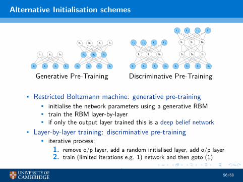
Generative Pre-Training Discriminative Pre-Training

• Restricted Boltzmann machine: generative pre-training• initialise the network parameters using a generative RBM• train the RBM layer-by-layer• if only the output layer trained this is a deep belief network

• Layer-by-layer training: discriminative pre-training• iterative process:

1. remove o/p layer, add a random initialised layer, add o/p layer2. train (limited iterations e.g. 1) network and then goto (1)

56/68

Example Systems(reference)

57/68

Autoencoders (Non-Linear Feature Extraction)

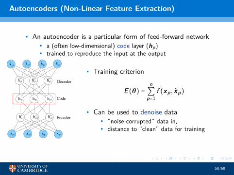
• An autoencoder is a particular form of feed-forward network• a (often low-dimensional) code layer (hp)• trained to reproduce the input at the output

p2 hp3

xp2 xp3xp1 xp4

Code

x x x xp1 p2 p3 p4

^ ^ ^ ^

hp1 hp2 hp3

hp1 hp2 hp3

(1) (1) (1)

(2) (2) (2)

Decoder

Encoder

hp1 h

• Training criterion

E(θ) =n∑p=1

f (xp, xp)

• Can be used to denoise data• “noise-corrupted” data in,• distance to “clean” data for training

58/68

Automatic Speech Recognition [22]

understand the CLDNN architecture are presented in Section 4. Re-sults on the larger data sets are then discussed in Section 5. Finally,Section 6 concludes the paper and discusses future work.

2. MODEL ARCHITECTURE

This section describes the CLDNN architecture shown in Figure 1.

2.1. CLDNN

Frame xt, surrounded by l contextual vectors to the left and r con-textual vectors to the right, is passed as input to the network. Thisinput is denoted as [xtl, . . . , xt+r]. In our work, each frame xt isa 40-dimensional log-mel feature.

First, we reduce frequency variance in the input signal by pass-ing the input through a few convolutional layers. The architectureused for each CNN layer is similar to that proposed in [2]. Specif-ically, we use 2 convolutional layers, each with 256 feature maps.We use a 9x9 frequency-time filter for the first convolutional layer,followed by a 4x3 filter for the second convolutional layer, and thesefilters are shared across the entire time-frequency space. Our pool-ing strategy is to use non-overlapping max pooling, and pooling infrequency only is performed [11]. A pooling size of 3 was used forthe first layer, and no pooling was done in the second layer.

The dimension of the last layer of the CNN is large, due to thenumber of feature-mapstimefrequency context. Thus, we add alinear layer to reduce feature dimension, before passing this to theLSTM layer, as indicated in Figure 1. In [12] we found that addingthis linear layer after the CNN layers allows for a reduction in pa-rameters with no loss in accuracy. In our experiments, we found thatreducing the dimensionality, such that we have 256 outputs from thelinear layer, was appropriate.

After frequency modeling is performed, we next pass the CNNoutput to LSTM layers, which are appropriate for modeling the sig-nal in time. Following the strategy proposed in [3], we use 2 LSTMlayers, where each LSTM layer has 832 cells, and a 512 unit projec-tion layer for dimensionality reduction. Unless otherwise indicated,the LSTM is unrolled for 20 time steps for training with truncatedbackpropagation through time (BPTT). In addition, the output statelabel is delayed by 5 frames, as we have observed with DNNs thatinformation about future frames helps to better predict the currentframe. The input feature into the CNN has l contextual frames tothe left and r to the right, and the CNN output is then passed to theLSTM. In order to ensure that the LSTM does not see more than 5frames of future context, which would increase the decoding latency,we set r = 0 for CLDNNs.

Finally, after performing frequency and temporal modeling, wepass the output of the LSTM to a few fully connected DNN layers.As shown in [5], these higher layers are appropriate for producing ahigher-order feature representation that is more easily separable intothe different classes we want to discriminate. Each fully connectedlayer has 1,024 hidden units.

2.2. Multi-scale Additions

The CNN takes a long-term feature, seeing a context of tl to t (i.e.,r = 0 in the CLDNN), and produces a higher order representationof this to pass into the LSTM. The LSTM is then unrolled for 20timesteps, and thus consumes a larger context of 20 + l. However,we feel there is complementary information in also passing the short-term xt feature to the LSTM. In fact, the original LSTM work in[3] looked at modeling a sequence of 20 consecutive short-term xt

C

...

D

D

L

L

Cconvolutional

layers

LSTMlayers

fullyconnected

layers

output targets

[xt-l,..., xt, ...., xt+r]

linearlayer

dimred

(1)

xt

(2)

Fig. 1. CLDNN Architecture

features, with no context. In order to model short and long-termfeatures, we take the original xt and pass this as input, along withthe long-term feature from the CNN, into the LSTM. This is shownby dashed stream (1) in Figure 1.

The use of short and long-term features in a neural network hasbeen explored previously (i.e., [13, 14]). The main difference be-tween previous work and ours is that we are able to do this jointlyin one network, namely because of the power of the LSTM sequen-tial modeling. In addition, our combination of short and long-termfeatures results in a negligible increase in the number of networkparameters.

In addition, we explore if there is complementarity betweenmodeling the output of the CNN temporally with an LSTM, as wellas discriminatively with a DNN. Specifically, motivated by work incomputer vision [10], we explore passing the output of the CNN intoboth the LSTM and DNN. This is indicated by the dashed stream(2) in Figure 1. This idea of combining information from CNN andDNN layers has been explored before in speech [11, 15], thoughprevious work added extra DNN layers to do the combination. Ourwork differs in that we pass the output of the CNN directly into theDNN, without extra layers and thus minimal parameter increase.

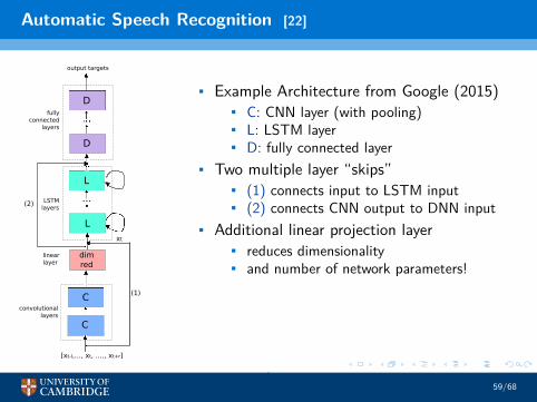
• Example Architecture from Google (2015)• C: CNN layer (with pooling)• L: LSTM layer• D: fully connected layer

• Two multiple layer “skips”• (1) connects input to LSTM input• (2) connects CNN output to DNN input

• Additional linear projection layer• reduces dimensionality• and number of network parameters!

59/68

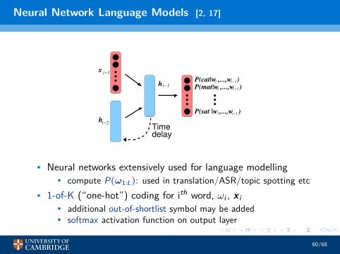
Neural Network Language Models [2, 17]

i−2h

i−1

Time

h

delay

xi−1

P(cat|w ,...,w )P(mat|w ,...,w )

P(sat |w ,...,w )1 i−1

1 i−1

1 i−1

• Neural networks extensively used for language modelling• compute P(ω1∶L): used in translation/ASR/topic spotting etc

• 1-of-K (“one-hot”) coding for ith word, ωi , x i• additional out-of-shortlist symbol may be added• softmax activation function on output layer

60/68

Neural Network Language Models [2, 17]

• Neural networks extensively used for language modelling• recurrent neural networks - complete word history

P(ω1∶L) =L∏i=1

P(ωi ∣ω1∶i−1) ≈L∏i=1

P(ωi ∣ωi−1, hi−2) ≈L∏i=1

P(ωi ∣hi−1)

• Input and output layer sizes can be very large• size of vocabulary (> 10K ), not an issue for input• output-layer (softmax) expensive (normalisation term)

• Issues that need to be addressed1. training: how to efficiently train on billions of words?2. decoding for ASR: how to handle dependence on complete

history?

61/68

Machine Translation: Encoder-Decoder Sequence Models

• Train a discriminative model from• x1∶L = x1, . . . ,xL: L-length input sequence (source language)• y1∶K = y1, . . . ,xK: K -length output (target language)

p(y1∶K ∣x1∶L) =K∏i=1

p(y i ∣y1∶i−1,x1∶L)

≈L∏i=1

p(y i ∣y i−1, hi−2, c)

• need to map x1∶L to a fixed-length vector

c = φ(x1∶L)

• c is a fixed length vector - like a sequence kernel

62/68

RNN Encoder-Decoder Model [9, 16]

x2

1h

xL

hLL−1h

x1

h0

Encoder

Decoder21 y

1h~

y

h~

KyyK−1

K−2

~

hK−1

• One form is to use hidden unit from acoustic RNN/LSTM

c = φ(x1∶L) = hL

• dependence on context is global via c - possibly limiting

63/68

Attention-Based Models [5, 4, 16]

Decoder

Attention ci+1ic

xt+1

th

xL

hLL−1h

xt

ht−1

Encoder

i+1yi y

hi−1 ih~ ~

64/68

Attention-Based Models

• Introduce attention layer to system• introduce dependence on locality i

p(y1∶K ∣x1∶L) ≈K∏i=1

p(y i ∣y i−1, hi−1, c i) ≈K∏i=1

p(y i ∣hi−1)

c i =L∑τ=1

αiτhτ ; αiτ =exp(eiτ)

∑Lj=1 exp(eij)

, eiτ = f e (hi−2,hτ)

• eiτ how well position i −1 in input matches position τ in output• hτ is representation (RNN) for the input at position τ

65/68

Image Captioning

Decoder21 y

1h~

y

h~

KyyK−1

K−2

~

hK−1

Encoder

• Encode-image as vector use a deep convolutional network• generate caption using recurrent network (RNN/LSTM)• all parameters optimised (using example image captions)

66/68

Conclusions

67/68

Is Deep Learning the Solution?

• Deep Learning: state-of-the-art performance in range of tasks• machine translation, image recognition/captioning,• speech recognition/synthesis ...

• Traditionally use two-stage approach to build classifier:1. feature extraction: convert waveform to parametric form2. modelling: given parameters train model

• Limitations in feature extraction cannot be overcome ...• integrate feature extraction into process• attempt to directly model/synthesise waveform (WaveNet)

• BUT• require large quantities of data (research direction)• networks are difficult to optimise - tuning required• hard to interpret networks to get insights• sometimes difficult to learn from previous tasks ...

68/68

[1] O. Abdel-Hamid, A.-R. Mohamed, H. Jiang, and G. Penn, “Applying convolutional neural networks conceptsto hybrid NN-HMM model for speech recognition,” in 2012 IEEE international conference on Acoustics,speech and signal processing (ICASSP). IEEE, 2012, pp. 4277–4280.

[2] Y. Bengio, R. Ducharme, P. Vincent, and C. Jauvin, “A neural probabilistic language model,” journal ofmachine learning research, vol. 3, no. Feb, pp. 1137–1155, 2003.

[3] C. Bishop, “Mixture density networks,” in Tech. Rep. NCRG/94/004, Neural Computing Research Group,Aston University, 1994.

[4] W. Chan, N. Jaitly, Q. V. Le, and O. Vinyals, “Listen, attend and spell,” CoRR, vol. abs/1508.01211, 2015.[Online]. Available: http://arxiv.org/abs/1508.01211

[5] J. Chorowski, D. Bahdanau, D. Serdyuk, K. Cho, and Y. Bengio, “Attention-based models for speechrecognition,” CoRR, vol. abs/1506.07503, 2015. [Online]. Available: http://arxiv.org/abs/1506.07503

[6] J. Chung, C. Gulcehre, K. Cho, and Y. Bengio, “Empirical evaluation of gated recurrent neural networks onsequence modeling,” arXiv preprint arXiv:1412.3555, 2014.

[7] J. Chung, K. Kastner, L. Dinh, K. Goel, A. C. Courville, and Y. Bengio, “A recurrent latent variable modelfor sequential data,” CoRR, vol. abs/1506.02216, 2015. [Online]. Available:http://arxiv.org/abs/1506.02216

[8] X. Glorot and Y. Bengio, “Understanding the difficulty of training deep feedforward neural networks.” inAistats, vol. 9, 2010, pp. 249–256.

[9] A. Graves, “Sequence transduction with recurrent neural networks,” CoRR, vol. abs/1211.3711, 2012.[Online]. Available: http://arxiv.org/abs/1211.3711

[10] A. Graves, A.-R. Mohamed, and G. Hinton, “Speech recognition with deep recurrent neural networks,” in2013 IEEE international conference on acoustics, speech and signal processing. IEEE, 2013, pp. 6645–6649.

[11] K. He, X. Zhang, S. Ren, and J. Sun, “Deep residual learning for image recognition,” CoRR, vol.abs/1512.03385, 2015. [Online]. Available: http://arxiv.org/abs/1512.03385

[12] G. Hinton, L. Deng, D. Yu, G. E. Dahl, A.-R. Mohamed, N. Jaitly, A. Senior, V. Vanhoucke, P. Nguyen,T. N. Sainath, et al., “Deep neural networks for acoustic modeling in speech recognition: The shared views offour research groups,” IEEE Signal Processing Magazine, vol. 29, no. 6, pp. 82–97, 2012.

68/68

[13] S. Hochreiter and J. Schmidhuber, “Long short-term memory,” Neural Comput., vol. 9, no. 8, pp.1735–1780, Nov. 1997.

[14] Y. LeCun and Y. Bengio, “Convolutional networks for images, speech, and time series,” The handbook ofbrain theory and neural networks, vol. 3361, no. 10, p. 1995, 1995.

[15] Y. LeCun, B. Boser, J. S. Denker, D. Henderson, R. E. Howard, W. Hubbard, and L. D. Jackel,“Backpropagation applied to handwritten zip code recognition,” Neural computation, vol. 1, no. 4, pp.541–551, 1989.

[16] L. Lu, X. Zhang, K. Cho, and S. Renals, “A study of the recurrent neural network encoder-decoder for largevocabulary speech recognition,” in Proc. INTERSPEECH, 2015.

[17] T. Mikolov, M. Karafiát, L. Burget, J. Cernocky, and S. Khudanpur, “Recurrent neural network basedlanguage model.” in Interspeech, vol. 2, 2010, p. 3.

[18] V. Nair and G. E. Hinton, “Rectified linear units improve restricted Boltzmann machines,” in Proceedings ofthe 27th International Conference on Machine Learning (ICML-10), 2010, pp. 807–814.

[19] T. Robinson and F. Fallside, “A recurrent error propagation network speech recognition system,” ComputerSpeech & Language, vol. 5, no. 3, pp. 259–274, 1991.

[20] S. Ruder, “An overview of gradient descent optimization algorithms,”http://sebastianruder.com/optimizing-gradient-descent/index.html, accessed: 2016-10-14.

[21] D. E. Rumelhart, G. E. Hinton, and R. J. Williams, “Parallel distributed processing: Explorations in themicrostructure of cognition, vol. 1,” D. E. Rumelhart, J. L. McClelland, and C. PDP Research Group, Eds.Cambridge, MA, USA: MIT Press, 1986, ch. Learning Internal Representations by Error Propagation, pp.318–362.

[22] T. N. Sainath, O. Vinyals, A. Senior, and H. Sak, “Convolutional, long short-term memory, fully connecteddeep neural networks,” in 2015 IEEE International Conference on Acoustics, Speech and Signal Processing(ICASSP). IEEE, 2015, pp. 4580–4584.

[23] M. Schuster and K. K. Paliwal, “Bidirectional recurrent neural networks,” IEEE Transactions on SignalProcessing, vol. 45, no. 11, pp. 2673–2681, 1997.

68/68

[24] N. Srivastava, G. E. Hinton, A. Krizhevsky, I. Sutskever, and R. Salakhutdinov, “Dropout: a simple way toprevent neural networks from overfitting.” Journal of Machine Learning Research, vol. 15, no. 1, pp.1929–1958, 2014.

[25] R. K. Srivastava, K. Greff, and J. Schmidhuber, “Highway networks,” CoRR, vol. abs/1505.00387, 2015.[Online]. Available: http://arxiv.org/abs/1505.00387

[26] P. Swietojanski and S. Renals, “Differentiable pooling for unsupervised acoustic model adaptation,”IEEE/ACM Transactions on Audio, Speech, and Language Processing, vol. PP, no. 99, pp. 1–1, 2016.

[27] C. Wu, P. Karanasou, M. Gales, and K. C. Sim, “Stimulated deep neural network for speech recognition,” inProceedings interspeech, 2016.

[28] H. Zen and A. Senior, “Deep mixture density networks for acoustic modeling in statistical parametric speechsynthesis,” in 2014 IEEE International Conference on Acoustics, Speech and Signal Processing (ICASSP).IEEE, 2014, pp. 3844–3848.

[29] C. Zhang and P. Woodland, “DNN speaker adaptation using parameterised sigmoid and ReLU hiddenactivation functions,” in Proc. ICASSP’16, 2016.

68/68