Send Orders for Reprints to reprints@benthamscience.ae

484 The Open Civil Engineering Journal, 2015, 9, 484-488

1874-1495/15 2015 Bentham Open

Open Access

Application of 3D-FSM Boundary Element Method in Stress and Displacement Analysis of Roadway

Wang Chong1,*, Liu Cheng-lun2 and Cui Xiaohua2

1Center of Modern Education, Shandong University of Science and Technology, Qingdao 266590, P.R. China 2College of Mining and Safety Engineering, Shandong University of Science and Technology, Qingdao 266590, P.R. China

Abstract: Conventional fictitious stress methods (FSM) employ numerical integration to calculate displacements or stresses on each element unit. The paper represents a kind of three-dimensional fictitious stress method adopting analytical integrals over triangular leaf elements instead of numerical integration and describes how to analyze stress and displacement of surrounding rock around roadway by the 3D-FSM. The results computed by this method were compared with the results obtained by Flac3d, which proved that it is a correct and rational method to solve three-dimensional mechanics problems especially about hole and crack in an elastic body.

Keywords: Fictitious stress method, analytical integrals, BEM, roadway, 3D-FSM.

1. INTRODUCTION

The solution to stresses and displacements of roadway surrounding rock and researches on the stability of surrounding sock are the major issues of rock mechanics studies representatively with traditional analytical methods including finite element method, finite difference method, discrete element method and boundary element method. Finite element method, difference method and discrete element method are based on three-dimensional finite spatial discretization. The degree of satisfaction of the solution depends on the size of the unit divided. Hence the solution process often takes a long time to reach a satisfactory solution. Despite several limitations, BEM greatly has unique advantages for solving the problems about spatially continuous elastomeric solid through rigorous integral transform (Green formula and Stokes Conversion), which changes three-dimensional problems into two-dimensional problems. A two-dimensional plane FSM method based on the integration of Kelvin solution was proposed by S.L.Crouch [1]. Afterwards, K.Kuriyama [2] gave the analytic solution of the integral equation based on Kelvin solution in 3D through space triangular facets division. Liu Chenglun [3] corrected errors in the literature [2], and compared the numerical solution of the 3D-FSM with analytical solution provided by Lame to a hollow sphere with constant forces that proved the rationality and validity of the method. The paper presents the method to calculate stresses and displacements of surrounding rock based on the studies of K.Kuriyama and Liu Chenglun, and compares the calculation results with the results by FLAC3d.

*Address correspondence to this author at Network and Information Center, Shandong University of Science and Technology, Qingdao 266590, P.R. China; Tel: +86 18561554929; E-mail:wcbaby@tom.com

2. INFLUENCE COEFFICIENTS

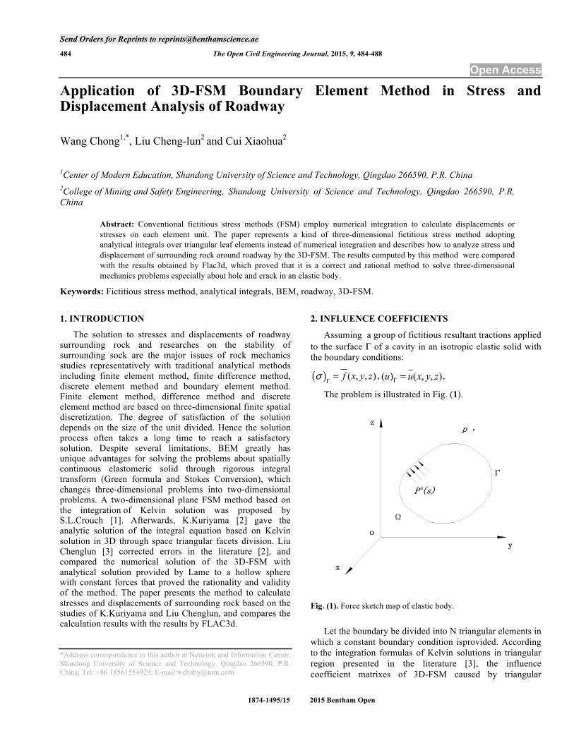
Assuming a group of fictitious resultant tractions applied to the surface Γ of a cavity in an isotropic elastic solid with the boundary conditions:

( ) ( , , )f x y zσΓ= , ( ) ( , , )u u x y zΓ = ,

The problem is illustrated in Fig. (1).

Fig. (1). Force sketch map of elastic body.

Let the boundary be divided into N triangular elements in which a constant boundary condition isprovided. According to the integration formulas of Kelvin solutions in triangular region presented in the literature [3], the influence coefficient matrixes of 3D-FSM caused by triangular

Application of 3D-FSM Boundary Element Method in Stress and Displacement Analysis The Open Civil Engineering Journal, 2015, Volume 9 485

element i can be written directly as Equations (1) and (2), and the parameters 1 17~f f , which are omitted and defined in the above literature, can be derived through the integration of the triangular element base on Kelvin’s solutions.

[ ]5 1 7 3

7 6 1 4

3 4 2 1

(3 4 )1 (3 4 )

16 (1 )(3 4 )

i

f f f zfQ f f f zf

Gzf zf zf f

νν

π νν

+ −⎡ ⎤⎢ ⎥= + −⎢ ⎥− ⎢ ⎥+ −⎣ ⎦

(1)

[ ]

3 14 4 17 2 11

3 16 4 15 2 12

3 9 4 10 2 8

4 17 3 16 13

13 2 12

[(1 2 ) ] 3 (1 2 ) 3 (1 2 ) 3(1 2 ) ] 3 [(1 2 ) 3 ] (1 2 ) 3(1 2 ) ] 3 (1 2 ) 3 [(1 2 ) 31[(1 2 ) 3 ] [(1 2 ) ] 3 38 (1 )

3 [(1 2 ) 3 ] [(

i

f f f f f ff f f f f ff f f f f f

Sf f f f zfGzf f f

ν ν νν ν νν ν νν νπ ν

ν

− − + − − − −− − − − + − −− − − − − − +

=− − + − − + −−

− − − + − 4 10

2 11 13 3 9

1 2 ) 3 ][(1 2 ) 3 ] 3 [(1 2 ) 3 ]

f ff f zf f f

νν ν

⎡ ⎤⎢ ⎥⎢ ⎥⎢ ⎥⎢ ⎥⎢ ⎥⎢ ⎥− +⎢ ⎥− − + − − − +⎢ ⎥⎣ ⎦

(2)

The components of displacements and stresses subjected to triangular element i at an arbitrary point can be written (in the local coordinate system of element i):

[ ]i

x xi

y i y

iz z

u pu Q p

u p

⎡ ⎤ ⎡ ⎤⎢ ⎥ ⎢ ⎥

= ⋅⎢ ⎥ ⎢ ⎥⎢ ⎥ ⎢ ⎥⎣ ⎦ ⎣ ⎦

(3),

[ ]

x

y ix

z ii y

xy iz

yz

zx

pS p

p

σσ

στ

τ

τ

⎡ ⎤⎢ ⎥⎢ ⎥

⎡ ⎤⎢ ⎥⎢ ⎥⎢ ⎥ = ⎢ ⎥⎢ ⎥⎢ ⎥⎢ ⎥ ⎣ ⎦⎢ ⎥

⎢ ⎥⎢ ⎥⎣ ⎦

(4)

Where ixp , i

yp , izp are the components of fictitious stresses

distributed at element i. 3. CO-ORDINATE TRANSFORMATIONS

A new local co-ordinate system was designed for the ith element, in which the points 1P , 2P , and 3P were arranged anticlockwise. 1P was taken as the origin of coordinates. The

direction of the vector A!"= P1P2! "!!!

is defined at x-axis, and

B!"= P1P3! "!!!

. Thus the direction of C!"= A!"! B!"

which is the normal direction of the planeOAB , is defined at z-axis. Hence, the direction of D

!"!=C!"! A!"

is defined at y-axis. The coordinate system i i iO x y is illustrated in Fig. (2). The local coordinate system of element j can be designed in the same way.

Fig. (2). local coordinate system of element i.

Assuming the direction cosines of the principal axes of element i are given as: 1 1 1( , , )i i il m n , 2 2 2( , , )i i il m n ,

3 3 3( , , )i i il m n , while 1 1 1( , , )j j jl m n , 2 2 2( , , )j j jl m n and

3 3 3( , , )j j jl m n for element j. ( , 1..3)jia i j = are defined as:

11 12 13 1 1 1 1 2 3

21 22 23 2 2 2 1 2 3

31 32 33 3 3 3 1 2 3

j j j i i i

j j j i i i

j j j i i i

a a a l m n l l la a a l m n m m ma a a l m n n n n

⎡ ⎤⎡ ⎤ ⎡ ⎤⎢ ⎥⎢ ⎥ ⎢ ⎥= ⎢ ⎥⎢ ⎥ ⎢ ⎥⎢ ⎥⎢ ⎥ ⎢ ⎥⎣ ⎦ ⎣ ⎦⎣ ⎦

Following this, the components of displacement under coordinate system j j jO x y transformed from i i iO x y can be given as equation (5),

11 12 13

21 22 23

31 32 33

[ ]

j i i

j i iji

j i i

x x xa a ay a a a y R y

a a az z z

⎡ ⎤ ⎡ ⎤ ⎡ ⎤⎡ ⎤⎢ ⎥ ⎢ ⎥ ⎢ ⎥⎢ ⎥= =⎢ ⎥ ⎢ ⎥ ⎢ ⎥⎢ ⎥⎢ ⎥ ⎢ ⎥ ⎢ ⎥⎢ ⎥⎣ ⎦⎣ ⎦ ⎣ ⎦ ⎣ ⎦

(5)

While the components of stresses under coordinate system j j jO x y can be calculated from the coordinate system i i iO x y

as represented in Equation (6).

4. SETTING UP SIMULTANEOUS EQUATIONS

Combining the influence coefficients and coordinate conversion shown above, the equations of displacement and stress can be detrmined at an arbitrary point in solid body resulting from uniform load in element i. Under the assumption that a model had the boundary geometrically equivalent to the wall of the hole and the boundary was divided into N triangular elements, the sum of the initial stress components and the stresses induced by the fictitious stresses equals to the pressure applied to the wall as shown in Equations (7) and (8).

xi (ξ)

zyi (η)

P1

P2

P3

O y

z

x

Oi

i

pzi

i

M(x ,y ,z )i i i

2 2 211 12 13 11 12 12 13 13 112 2 221 22 23 21 22 22 23 23 212 2 231 32 33 31 32 32 33 33 31

11 21 12 22 13 23 11 22 12 21 12 23 22 13 13 21

2 2 22 2 22 2 2

( ) ( ) (

jxjy

jzjxy

jyz

jxz

a a a a a a a a aa a a a a a a a aa a a a a a a a aa a a a a a a a a a a a a a a a a

σσ

στ

τ

τ

⎡ ⎤⎢ ⎥⎢ ⎥⎢ ⎥⎢ ⎥ =⎢ ⎥ + + +⎢ ⎥⎢ ⎥⎢ ⎥⎢ ⎥⎣ ⎦

23 11

21 31 22 32 23 33 21 32 31 22 22 33 32 23 23 31 33 21

31 11 32 12 33 13 11 32 31 12 12 33 32 13 31 13 33 11

[)

( ) ( ) ( )( ) ( ) ( )

ixiy

iz

ijixy

iyz

ixz

Ta

a a a a a a a a a a a a a a a a a aa a a a a a a a a a a a a a a a a a

σσ

στ

τ

τ

⎡ ⎤⎡ ⎤ ⎢ ⎥⎢ ⎥ ⎢ ⎥⎢ ⎥ ⎢ ⎥⎢ ⎥ ⎢ ⎥ =⎢ ⎥ ⎢ ⎥⎢ ⎥ ⎢ ⎥⎢ ⎥+ + + ⎢ ⎥⎢ ⎥ ⎢ ⎥+ + +⎢ ⎥⎣ ⎦ ⎢ ⎥⎣ ⎦

] (6)

ixiy

izixy

iyz

ixz

σσ

στ

τ

τ

⎡ ⎤⎢ ⎥⎢ ⎥⎢ ⎥⎢ ⎥⎢ ⎥⎢ ⎥⎢ ⎥⎢ ⎥⎢ ⎥⎣ ⎦

486 The Open Civil Engineering Journal, 2015, Volume 9 Chong et al.

1

j ix xnj iy ji ji y

ij iz z

u pu R Q p

u p=

⎡ ⎤ ⎡ ⎤⎢ ⎥ ⎢ ⎥

⎡ ⎤ ⎡ ⎤= ⋅ ⋅⎢ ⎥ ⎢ ⎥⎣ ⎦ ⎣ ⎦⎢ ⎥ ⎢ ⎥⎣ ⎦ ⎣ ⎦

∑ (7)

1

jxjy i

xj nz i

ji ji yjixy i

zjyz

jzx

pT S p

p

σσ

στ

τ

τ

=

⎡ ⎤⎢ ⎥⎢ ⎥

⎡ ⎤⎢ ⎥⎢ ⎥⎢ ⎥ ⎡ ⎤ ⎡ ⎤= ⋅ ⋅ ⎢ ⎥⎣ ⎦ ⎣ ⎦⎢ ⎥⎢ ⎥⎢ ⎥ ⎣ ⎦⎢ ⎥

⎢ ⎥⎢ ⎥⎣ ⎦

∑ (8)

Where jiT⎡ ⎤⎣ ⎦ is the local transformation matrix with respect

to the stress from i i iO x y to j j jO x y ; jiR⎡ ⎤⎣ ⎦ is the local

transformation matrix with respect to displacement; jiS⎡ ⎤⎣ ⎦ is the influence coefficient matrix with respect to stress and

jiQ⎡ ⎤⎣ ⎦ with respect to displacement from element i to element j. 5. EXAMINATION IN EXCAVATING ROADWAY

Let the roadway boundary be divided into n elements in triangular leaf shape connecting with each other. Displacement and stress induced by element i at the center of gravity of the jth element can be given by integrations of expressions (7) and (8). Assume that the components of the fictitious stress at element i are evenly distributed as i

xp , iyp ,

izp , the stress in rocks will be changed once the roadway is

excavated. The re-distributed stress equals the sum of initial stress 0σ and induced stress 1σ , viz. 0 1σ σ σ= + .

There are 3N unknown variables ixp , i

yp , izp (i=1~n). For

the solutions, 3n simultaneous equations are designed as the following Equation(9):

0 0

01

0

, ( 1 ~ )

j j iz xn

j iyz ji ji y

ij izx z

p pT S p j n

p

στ

τ=

⎡ ⎤ ⎡ ⎤−⎢ ⎥ ⎢ ⎥

⎡ ⎤ ⎡ ⎤− = ⋅ ⋅ =⎢ ⎥ ⎢ ⎥⎣ ⎦ ⎣ ⎦⎢ ⎥ ⎢ ⎥−⎣ ⎦ ⎣ ⎦

∑ (9)

Where 0jp is the internal fluid pressure applied to ith

element on the boundary; 0jzσ is the initial normal stress in

local coordinate system j and 0jyzτ , and 0

jzxτ are the initial

shear stresses in local coordinate system j. The stress and displacement induced by excavation at an arbitrary point on the boundary are equal to the initial stress in magnitude but opposite in direction as shown in Equation (9). Solving the equations and with the value of i

xp , iyp , i

zp ( 1.. )i n= , all six components of the stress can be calculated at an arbitrary point p as shown in Equation (10), and the components of displacement are shown as Equation (11) :

0

0

0

1 0

0

0

p pxx xxp p

iyy yyxp pnizz zz

pi pi yp pixy xyi

p pzyz yzp pxz xz

pT S p

p

σ σσ σσ σσ σσ σσ σ

=

⎡ ⎤ ⎡ ⎤⎢ ⎥ ⎢ ⎥⎢ ⎥ ⎢ ⎥⎡ ⎤⎢ ⎥ ⎢ ⎥⎢ ⎥

⎡ ⎤ ⎡ ⎤= +⎢ ⎥ ⎢ ⎥⎢ ⎥⎣ ⎦ ⎣ ⎦⎢ ⎥ ⎢ ⎥⎢ ⎥⎢ ⎥ ⎢ ⎥⎣ ⎦⎢ ⎥ ⎢ ⎥⎢ ⎥ ⎢ ⎥⎣ ⎦ ⎣ ⎦

∑ (10)

1

p ix xnp iy pi pi y

ip iz z

u pu R Q p

u p=

⎡ ⎤ ⎡ ⎤⎢ ⎥ ⎢ ⎥

⎡ ⎤ ⎡ ⎤= ⋅ ⋅⎢ ⎥ ⎢ ⎥⎣ ⎦ ⎣ ⎦⎢ ⎥ ⎢ ⎥⎣ ⎦ ⎣ ⎦

∑ (11)

6. A NUMERICAL EXAMPLE

Certain part of the tunnel was excavated at the layer of 500 meters below the surface which is of 40m long, 5m wide and the side wall is 3m high. The upper part of the tunnel is a semi-circular dome, as shown in Fig. (3) (the bottom lies in the plane z=-1).

Fig. (3). Division of the boundary of the Tunnel.

The surrounding rock is homogeneous continuous medium, with 10000E Mpa= and 0.26v = . According to Heim geological assumptions, the original rock stresses are:

z ghσ ρ= (12)

0.33331x y z zvv

σ σ σ σ= = =−

(13)

The boundary of the tunnel is divided into 1440 units. According to the problem, the boundary conditions can be given as:

( )0 0 1..j i np = = ,

0

0

00

0

0

0

jx

jy

jzjz j

jxy

jyz

jxz

T

σσσ

στττ

⎡ ⎤⎢ ⎥⎢ ⎥⎢ ⎥

⎡ ⎤= ⎢ ⎥⎣ ⎦ ⎢ ⎥⎢ ⎥⎢ ⎥⎢ ⎥⎣ ⎦

,

Application of 3D-FSM Boundary Element Method in Stress and Displacement Analysis The Open Civil Engineering Journal, 2015, Volume 9 487

0 0 0j jyz zxτ τ= = ,

Where 0jxσ , 0jyσ , 0jzσ , 0jxyτ , 0jzyτ , and 0jzxτ are the components of initial stress at point j which can be calculated from formulas (12) and (13). jT⎡ ⎤⎣ ⎦ is the coordinate conversion matrix obtained from world coordinate system to form local coordinate system j. 0

jzσ ,

0jzxτ and 0

jzyτ are the initial stresses at the gravity point of

element j in local coordinate system j. Evidently, the shear stresses on the boundary are all zero. Solving equation (9) with boundary conditions shown above, fictitious stresses i

xp, i

yp , izp ( 1.. )i n= can be computed and the stress and

displacement at an arbitrary point p can be computed with formulas(10) and (11).

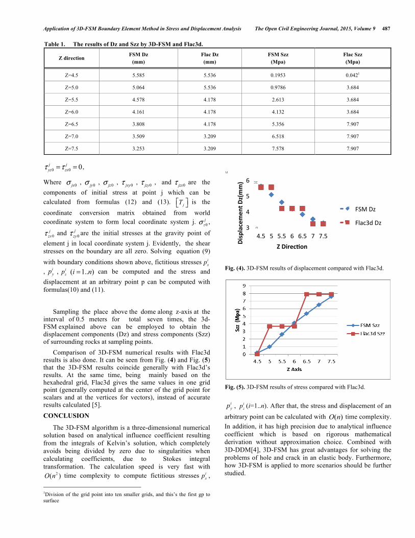
Sampling the place above the dome along z-axis at the interval of 0.5 meters for total seven times, the 3d-FSM explained above can be employed to obtain the displacement components (Dz) and stress components (Szz) of surrounding rocks at sampling points. Comparison of 3D-FSM numerical results with Flac3d results is also done. It can be seen from Fig. (4) and Fig. (5) that the 3D-FSM results coincide generally with Flac3d’s results. At the same time, being mainly based on the hexahedral grid, Flac3d gives the same values in one grid point (generally computed at the center of the grid point for scalars and at the vertices for vectors), instead of accurate results calculated [5]. CONCLUSION

The 3D-FSM algorithm is a three-dimensional numerical solution based on analytical influence coefficient resulting from the integrals of Kelvin’s solution, which completely avoids being divided by zero due to singularities when calculating coefficients, due to Stokes integral transformation. The calculation speed is very fast with

2( )O n time complexity to compute fictitious stresses ixp ,

1Division of the grid point into ten smaller grids, and this’s the first gp to surface

iyp , i

zp (i=1..n). After that, the stress and displacement of an arbitrary point can be calculated with ( )O n time complexity. In addition, it has high precision due to analytical influence coefficient which is based on rigorous mathematical derivation without approximation choice. Combined with 3D-DDM[4], 3D-FSM has great advantages for solving the problems of hole and crack in an elastic body. Furthermore, how 3D-FSM is applied to more scenarios should be further studied.

Table 1. The results of Dz and Szz by 3D-FSM and Flac3d.

Z direction FSM Dz

(mm) Flac Dz (mm)

FSM Szz (Mpa)

Flac Szz (Mpa)

Z=4.5 5.585 5.536 0.1953 0.0421

Z=5.0 5.064 5.536 0.9786 3.684

Z=5.5 4.578 4.178 2.613 3.684

Z=6.0 4.161 4.178 4.132 3.684

Z=6.5 3.808 4.178 5.356 7.907

Z=7.0 3.509 3.209 6.518 7.907

Z=7.5 3.253 3.209 7.578 7.907

Fig. (4). 3D-FSM results of displacement compared with Flac3d.

Fig. (5). 3D-FSM results of stress compared with Flac3d.

3  

4  

5  

6  

4.5   5   5.5   6   6.5   7   7.5  Displacemen

t  Dz(mm)

Z  Direc2on

FSM  Dz  

Flac3d  Dz  

488 The Open Civil Engineering Journal, 2015, Volume 9 Chong et al.

CONFLICT OF INTEREST

The author confirms that this article content has no conflict of interest.

ACKNOWLEDGEMENTS

Declared none.

REFERENCES [1] S. L. Crouch, and A. M. “Starfield, Boundary Element Methods In

Solid Mechanics”, Unwin Hyman: London, 1974, pp. 25-26. [2] K. Kuriyama, Y. Mizuta, H. Mozumi, and T. Watanabe, “Three-d-

imensional elastic analysis by the boundary element method with

analytical integrations over trianguluar leaf elements”, Interna-tional Journal of Rock Mechanics and Mining, vol. 32, no. 1, pp. 77-83, 1995.

[3] C. Liu, Y. Mizuta, and K. Kuriyama, “Anaytical integrations for three-dimensional fictitious stress method based on kelvin solution”, Journal of the Mining and Materials Processing Institute of Japan, vol. 115, pp. 719-724,1999.

[4] K. Kuriyama, and Y. Mizuta, “Three-dimensional elastic analysis by the displacement discontinuity method with boundary division into triangular leaf elements”, Sciences and Genomics Abstracts, vol. 30, no. 2, pp. 111-123, 1993.

[5] C. Liu, G. Li, K. Kuriyama, and Y. Mizuta, “Development of a computer program for inhomogeneous modeling using 3-D BEM with analytical integration and its application to rock slope stability evaluation”, International Journal of Rock Mechanics and Mining, vol. 42, no. 1, pp. 137-144.

Received: April 18, 2015 Revised: May 30, 2015 Accepted: June 05, 2015 © Chong et al.; Licensee Bentham Open.

This is an open access article licensed under the terms of the Creative Commons Attribution Non-Commercial License (http://creativecommons.org/licenses/ by-nc/4.0/) which permits unrestricted, non-commercial use, distribution and reproduction in any medium, provided the work is properly cited.