45315 baseline graphite characterization report

INL/EXT-18-45315Revision 0

Graphite Characterization:Baseline Variability Analysis Report

Mitch PlummerAndrea Mack

June 2018

DISCLAIMERThis information was prepared as an account of work sponsored by an

agency of the U.S. Government. Neither the U.S. Government nor any agency thereof, nor any of their employees, makes any warranty, expressed or implied, or assumes any legal liability or responsibility for the accuracy, completeness, or usefulness, of any information, apparatus, product, or process disclosed, or represents that its use would not infringe privately owned rights. References herein to any specific commercial product, process, or service by trade name, trade mark, manufacturer, or otherwise, does not necessarily constitute or imply its endorsement, recommendation, or favoring by the U.S. Government or any agency thereof. The views and opinions of authors expressed herein do not necessarily state or reflect those of the U.S. Government or any agency thereof.


Graphite Characterization: Baseline Variability Analysis Report

Mitch PlummerAndrea Mack

June 2018

Idaho National LaboratoryART Program

Idaho Falls, Idaho 83415

http://www.inl.gov

Prepared for theU.S. Department of EnergyOffice of Nuclear Energy

Under DOE Idaho Operations OfficeContract DE-AC07-05ID14517

INL ART Program



June 2018

v

EXECUTIVE SUMMARYThe Idaho National INL’s Baseline Material Property program provides

many measurements of different material properties on a variety of nuclear graphite grades being investigated for irradiation-induced changes in material properties. The baseline material properties provide an unirradiated reference for comparison with measurements of those properties after irradiation. This study describes how uncertainty, or variance, in estimates of important material properties, like compressive strength, may depend on sample size, sample distribution and parameter estimation methods. Compressive strength data from two large collections of specimens from a billet of PCEA graphite (sample size =230) and a billet of IG-110 graphite (sample size = 48) are used to illustrate these dependencies. The grades of graphite used represent approximate end members in terms of relative variability in strength measurements.

Monte Carlo simulation and bootstrapping methods were used to examine variance in Weibull-parameter estimates as a function of sample size. Results were consistent with what previous statistical analyses have shown about the relationship between sample size and width of the confidence interval for maximum likelihood (ML) estimated parameters when samples are repeatedly drawn from a Weibull distribution. As a function of sample size, the precision of the modulus estimate increases faster than that of the characteristic strength. Themodulus maximum likelihood estimates (MLEs) are biased for low sample sizes.

The American Society for Testing and Materials document ASTM D7846-16provides equations that describe the dependence of the variance of parameterMLEs on sample size. Using the same methodology, we show that the polynomials provided for variance dependence on sample size are inaccurate for sample sizes greater than ~120. We provide approximations to that relationship that illustrate relative constancy for sample size > ~10, in the logspace relationship of the modulus variance and the log transformed characteristic strength variance.

Bootstrapping provided a means of comparing Weibull parameters obtained using ASME’s guidance for specimen collection to those obtained using different weighting in a case where strength is related to position in a billet and to grain orientation and a single distribution is used to characterize the billet. ASME specifies that samples be collected with equal representation in all locations and grain orientations. Parameter values obtained using ASME’s method were different from those obtained using random sampling of the complete data sets, and this was particularly true for the PCEA data. In addition, while the ASME approach yielded more conservative parameters for the PCEA data, the opposite was true for the IG-110 data. The difference observed for the PCEA data set likely reflects the larger number of against-grain specimens collected, which had generally higher strength than the with-grain specimens. This emphasizes the importance of the dependence of strength on location or grain orientation and suggests that it may be prudent to weight specimen collection toward the weaker subgroups if a conservative estimate as desired, as the equal weighting method recommended by ASME would will not always provide the most conservative Weibull parameters. Because spatial correlations commonly exist in certain grades of graphite, future work may involve developing a methodology for parameter inference that relaxes the assumption of independent specimens.

vi

ASTM and ASME codes recommend different parameter estimation methods and models of the Weibull distribution in different situations. Descriptions of the effects on parameter estimates for the example billets used in this study provide an example of how the method may affect the parameter estimate, and how—in this case—that compares to differences due to other factors, such as sample size and dependence on grain orientation or sample location.

vii

CONTENTS

EXECUTIVE SUMMARY .......................................................................................................................... v

ACRONYMS............................................................................................................................................... xi

1. INTRODUCTION.............................................................................................................................. 1

2. BACKGROUND................................................................................................................................ 2

3. METHODS......................................................................................................................................... 4 3.1 Approximations to Define Dependence of Parameter Estimates on Sample Size ................... 8

4. STRENGTH MEASUREMENTS FROM BILLETS OF PCEA AND IG-110 GRADE GRAPHITE ........................................................................................................................................ 9 4.1 Experimental Measurements.................................................................................................... 9

5. RESULTS......................................................................................................................................... 11 5.1 Effects of Spatial Trends in Material Strength on Fitted Weibull Parameters ....................... 12 5.2 Effects of Sampling Balance on Fitted Weibull Parameters .................................................. 17 5.3 Effects of Estimation Methods on Fitted Weibull Parameters ............................................... 20 5.4 Comparison of Effects on an Example Design Factor ........................................................... 22

6. CONCLUSIONS .............................................................................................................................. 22

7. REFERENCES................................................................................................................................. 24

FIGURESFigure 1. Theoretical density functions for the three example Weibull distributions, where the

load is normalized to the characteristic strength and the density is multiplied by that value.............................................................................................................................................. 4

Figure 2. Box plot giving true parameter (green horizontal line), first and third quantiles (box), upper and lower whiskers (line extent) and outliers of the distribution of MLE scale (top) and shape (bottom) parameters. ........................................................................................... 5

Figure 3. Unbiasing factors for the Weibull modulus, as tabulated in ASTM D7846-16............................. 6

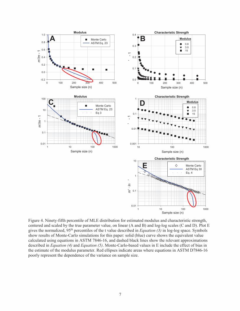
Figure 4. Ninety-fifth percentile of MLE distribution for estimated modulus and characteristic strength, centered and scaled by the true parameter value, on linear (A and B) and log-log scales (C and D). Plot E gives the normalized, 95th percentiles of the t value described in Equation (3) in log-log space. Symbols show results of Monte-Carlo simulations for this paper: solid (blue) curve shows the equivalent value calculated using equations in ASTM 7846-16, and dashed black lines show the relevant approximations described in Equation (4) and Equation (5). Monte-Carlo-based values in E include the effect of bias in the estimate of the modulus parameter. Red ellipses indicate areas where equations in ASTM D7846-16 poorly represent the dependence of the variance on sample size. ......................................................................................................... 7

viii

Figure 5. Cylindrical extruded billets of PCEA graphite are sectioned into seven slabs along the z-axis and quartered into sub-wedges, from which test specimens are extracted in parallel, transverse, and radial orientations. ............................................................................... 10

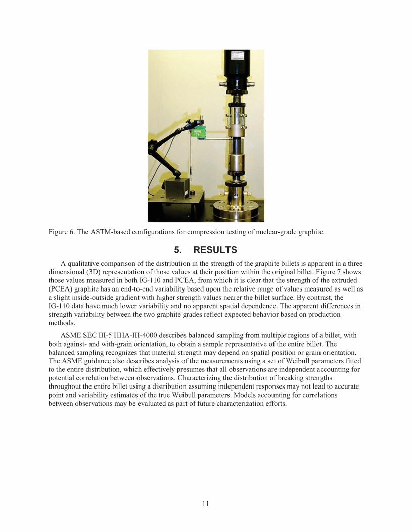
Figure 6. The ASTM-based configurations for compression testing of nuclear-grade graphite................. 11

Figure 7. Three-dimensional display of compressional strength at failure measurements from PCEA and IG-110 billets, representing 169 specimens (PCEA) and 48 specimens (IG-110), respectively................................................................................................................. 12

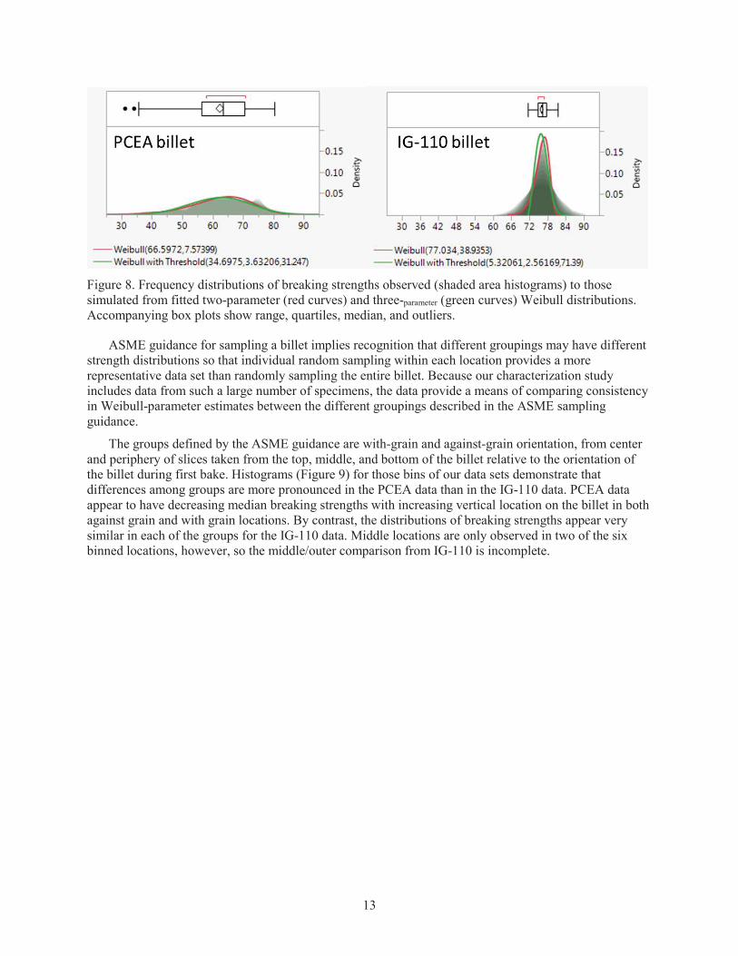
Figure 8. Frequency distributions of breaking strengths observed (shaded area histograms) to those simulated from fitted two-parameter (red curves) and three-parameter (green curves) Weibull distributions. Accompanying box plots show range, quartiles, median, and outliers. ....................................................................................................................................... 13

Figure 9. Histograms of observed breaking strengths for a billet of PCEA graphite and a billet of IG-110 graphite, grouped to reflect potential differences that are combined by sampling according to ASME/BPVC SEC III-5 – Section III, Division 5 High Temperature Reactors, Article HHA III 4000.................................................................................................. 14

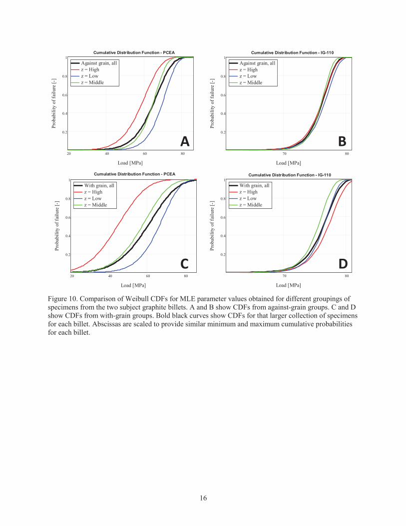
Figure 10. Comparison of Weibull CDFs for MLE parameter values obtained for different groupings of specimens from the two subject graphite billets. A and B show CDFs from against-grain groups. C and D show CDFs from with-grain groups. Bold black curves show CDFs for that larger collection of specimens for each billet. Abscissas are scaled to provide similar minimum and maximum cumulative probabilities for each billet. ........................................................................................................................................... 16

Figure 11. Confidence intervals derived from bootstrapping of PCEA and IG-110 data at different sample sizes, via random sampling of the complete set of observations (gray shading) and random sampling of the same set, but with each set containing subsamples balanced according to the ASME guidance for sampling (blue shading). Solid lines indicate median parameter values; vertical reference lines are located at the ASME recommended sample size of 24 and at the sample size of the full collection of specimens from each billet. ........................................................................................................ 19

Figure 12. Cumulative distribution functions for our two subject graphite billets, using ML-derived parameters calculated from all observations determined in our characterization effort (red curves) and by bootstrapping with sampling guided by ASME recommendations for sampling with respect to location and grain-orientation (blue curves). Graphs are shown with linearly scaled probability (A and B) and log-scaled probability (C and D). Abscissas are scaled to provide similar minimum and maximum cumulative probabilities for each billet. ..................................................................................... 20

Figure 13. PCEA and IG-110 billets compressive-strength data plotted on rank-regression plots. Curves illustrate different methods of parameter estimation; MLE=maximum likelihood estimation; RR=rank regression; JMP = SAS JMP software calculation; RR non-lin = non-linear fit to match observations in rank-regression space; RR & MLE = ML for modulus and characteristic strength parameters following non-linear regression for location parameter in rank regression space. Abscissas are scaled to provide similar minimum and maximum cumulative probabilities for each billet. ............................................. 21

Figure 14. Cumulative distribution functions for the PCEA (A) and IG-110 (B) billets, using parameters calculated from all observations determined in our characterization effort, but using different estimation methods. MLE = maximum likelihood estimators; RR = rank regression; JMP 1 = JMP Distribution procedure; JMP 2 = JMP Reliability

ix

procedure; RR-MLE = rank regression to fit location parameter, followed by MLE for remaining parameters. Abscissas are scaled to provide similar minimum and maximum cumulative probabilities for each billet. ..................................................................................... 22

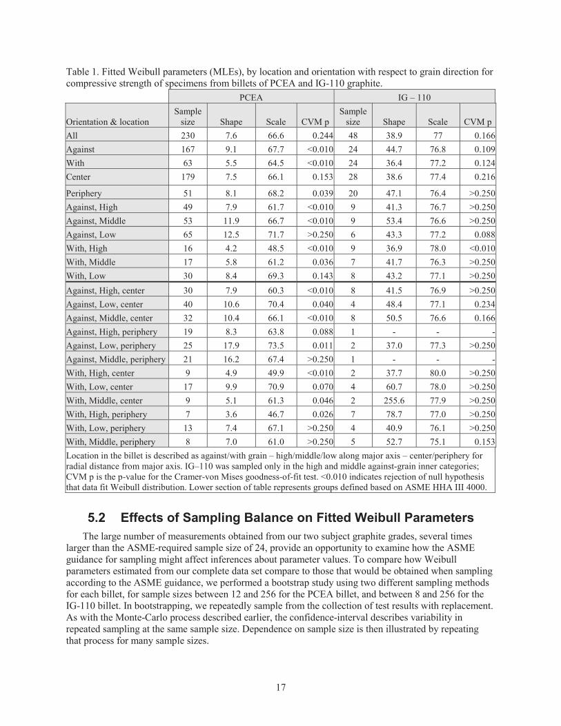
TABLETable 1. Fitted Weibull parameters (MLEs), by location and orientation with respect to grain

direction for compressive strength of specimens from billets of PCEA and IG-110graphite. ...................................................................................................................................... 17

xi

ACRONYMSART Advanced Reactor Technologies

ASME American Society of Mechanical Engineers

ASTM American Society for Testing and Materials

CDF cumulative distribution function

DOE Department of Energy

HTGR high-temperature gas-cooled reactor

HTR high-temperature reactor

IQR interquartile range

JMP SAS JMP software calculation

JMP 1 JMP distribution

JMP 2 JMP reliability procedure

ML maximum likelihood

MLE maximum likelihood estimate

POF probability of failure

R&D research and development

RR rank regression

1


1. INTRODUCTIONHigh-purity graphite is the core structural material of choice in the High Temperature Reactor (HTR)

design; a graphite-moderated, helium- or molten-salt-cooled design that is capable of producing process heat for power generation and for industrial processes that require temperatures higher than the outlet temperatures of present nuclear reactors. Nuclear-grade graphite is an ideal material for this design based on its thermal stability, neutron moderation, machinability, and low cost. However, the material properties of nuclear graphite are more variable, especially the new grades developed for advanced reactor designs. For example, the quasi-brittle mechanical properties of graphite have been demonstrated to exhibit a relatively large amount of variability in measured strength levels. Breaking strengths depend on the inherent defect structure, composed of boundaries between filler particles, pores, voids, inclusions, and cracks that are present. Therefore, the measured mechanical properties in various graphite grades is strongly a function of the size distribution of these defects and their relative orientation with respect to the stress axis. While characterization of past nuclear-grade graphite was extensive, historical nuclear grades no longer exist(Allen et al. 2008). New grades with little operational experience must be fabricated, characterized, and irradiated in order to demonstrate that current grades of graphite exhibit acceptable irradiated and unirradiated properties for the thermomechanical design of HTR core components.

The Department of Energy (DOE) Advanced Reactor Technologies (ART) Graphite Research and Development program seeks to understand the irradiated and unirradiated properties of these relatively new grades of nuclear graphite. The Advanced Graphite Creep experiment of that program is designed to understand how variability in irradiation temperatures, dose, and levels of stress affect nuclear-grade graphite material. The Baseline Graphite Characterization project complements that experiment by characterizing unirradiated graphite material properties to establish the batch-to-batch, billet-to-billet, and within-billet variability of the material across different grades. This characterization will establish a comprehensive set of material properties data, collected in accordance with the American Society of Mechanical Engineers (ASME) Nuclear Quality Assurance program (NQA-1-2008/1s-2009). This baseline material properties data set be used in the design and licensing of HTR core components and as a reference for comparison to irradiated material properties. Nuclear graphite grades included in the data set differ ingrain size, fabrication process, coke source, and production readiness (i.e., how long the specific grade has been in large-scale production). While all grades are “production ready,” meaning that they have been developed enough to produce full-size batches of billets capable of providing enough material to fill a reactor core, some of the grades are more established than others in terms of general testing and use.

As part of the Baseline Graphite Characterization project, this report describes methodologies to assess within-billet variability in material properties, applies these methodologies to two newer nuclear-grade graphite materials, and compares material properties of these newer grades to those of more established grades.

Qualification of nuclear reactor designs has historically relied upon representative material-property data for reactor-grade graphite, particularly tensile and compressive strength, to ensure the structural integrity of the core. Due to the quasi-brittle nature of graphite, ASME codes specify methods for sample collection and modeling of strength variables using the Weibull strength-distribution method. The ASME code for design of graphite reactor-core components requires characterization using either a two- or three-parameter Weibull distribution and provides guidelines for design based on anticipated stress and probability of failure determined from the Weibull parameters. Complementing the ASME code is the American Society for Testing and Materials (ASTM) standard (ASTM D7846-16), which describes a specific methodology for estimating the parameters of the two-parameter Weibull distribution.

2

In this study, the dependence of Weibull-parameter variability within a single billet is evaluated as a function of graphite type and the number and location of compressive strength measurements. Understanding how uncertainty in mechanical strength Weibull parameters varies as a function of the number and position of measurements will provide guidance for qualification of newer nuclear-grade graphite materials and will enable the ART Graphite Baseline project to quantify how additional testing might serve to improve characterization of material properties.

2. BACKGROUNDThe Energy Policy Act of 2005 mandated the construction and operation of a high-temperature

gas-cooled reactor (HTGR) by 2021. As a result of the Act, the U.S. Congress chose to develop what became known as the Next-Generation Nuclear Plant, which was to be a high-temperature gas reactor (HTGR) designed to produce sufficiently high-temperature process heat for hydrogen production, as well as energy for electricity generation. High-purity synthetic graphite is the core structural material of choice for HTR designs due to its capacity as both neutron moderator and reflector, stability at high temperature, machinability, and low cost. Understanding the material properties of nuclear-grade graphite is thus critical to development of robust HTGR designs. Unfortunately, while the general manufacturing processes necessary for producing nuclear-grade graphite are known, historical nuclear-grades are no longer produced(Allen et al. 2008). New grades must be fabricated, characterized, and irradiated to demonstrate that they exhibit acceptable irradiated and unirradiated properties for the thermomechanical design of HTGR core components. Accordingly, the DOE ART program initiated a Graphite Research and Development program in 2005 to provide material data (both unirradiated and irradiated data) necessary for the eventual utilization of these graphite grades for nuclear core components in HTR applications.

The Baseline Graphite Characterization program endeavors to provide a high-resolution (large sample size of multiple precise measurements) data set describing as-manufactured mechanical and physical baseline (unirradiated) properties in nuclear-grade graphite. The dataset is also a reference for other characterization studies to illustrate how uncertainty in material properties changes with sample size. The program also collected data on individual specimen source, position, and orientation information in order to provide comparisons in distributional properties between different positions within a single billet.

The two grades of graphite considered in this study, PCEA and IG-110, represent approximatelyopposite ends of the spectrum of variability of material properties. PCEA is a new petroleum-coke gradeproduced by GrafTech with a medium (~800 and formed via an extrusion process. It was originally designed to replicate the historical H451 grade used in previous prismatic HTGR designs. IG-110 is a petroleum-coke graphite with a superfine isotropic microstructure from Toyo Tanso, formed via cold isostatic molding. IG-110 might be considered the most established of all nuclear grades currently available; it has been used in prismatic and pebble-bed applications and has been discussed for molten-salt applications.

Compressive strength at failure was chosen as the graphite characterization measure for this study due to the very large datasets for each grade. Strength at failure is a critical design criterion for graphite core components and may be used as a comparison of the relative quality of two materials, the prediction of the probability of failure for a structure of interest, or to establish load limits for a particular level of probability of failure (ASTM D7846-16).

The Weibull distribution is an extreme value distribution which Weibull (1951) considered to provide the appropriate mathematical description of the size effect of failures in solids. In a review of statisticalmodels of fracture relevant to nuclear-grade graphite, Nemeth and Bratton (2011) concluded that the Weibull distribution is the most appropriate statistical distribution to model the stochastic behavior of the strength of graphite. That conclusion is consistent with analysis methodologies described in ASME and ASTM documents describing analysis of graphite strength at failure; therefore, the Weibull distribution was used in this work to model the distribution of breaking strengths within a billet.

3

The two-parameter Weibull distribution equation is( ) = ; , > 0, 0( ) = 0 , < 0 (1)

where m is the Weibull modulus, or shape, parameter, is the characteristic strength, or scale parameter, and x is the compressive strength at failure. The Weibull distribution is presently the only statistical analysis technique that is specifically adopted as an ASTM standard (ASTM D7846-16) for the evaluation of graphite mechanical properties. The ASME code for design of graphite reactor core components describes estimation methods for both two- and three-parameter Weibull distributions to model failure of a graphite component. In a three-parameter Weibull distribution, a third “location” parameter defines an effective minimum strength of the material. In this study, we focus on the ASTM-referenced method, maximum likelihood (ML) estimation of the two-parameter Weibull distribution, and how uncertainty in the parameter estimates varies with sample size. We also compare that uncertainty to how parameter estimates are affected by specimen distribution, estimation method, and choice of Weibull model.

As described in ASTM D7846-16, Weibull parameter estimates should be consistent and efficient,meaning that as the amount of information in the sample increases, the estimator should approach the true parameter with the minimum sampling variance of all other estimators. The uncertainty in estimates depends on the number of samples. As the number of specimens (sample size) increases, the uncertainty in the parameter estimates decreases, narrowing the width of confidence intervals for a specified level of statistical significance. In this report, we examine the bias and uncertainty of parameter estimates found using a large sample of strength-at-failure measurements from two billets of different grades of graphitecharacterized as part of the Baseline Graphite Characterization effort. While other studies (Price 1976) have used large collections of measurements from a single block of graphite (2000 tensile and four-point bend tests on a single log of Great Lakes Carbon Corporation grade H-451) to examine variability of mechanical properties and dependence on location and grain orientation, this is, to our knowledge, the first such large-scale sampling study of modern nuclear-grade graphite.

Previous studies have examined the bias introduced by different estimators, and described methods of reducing that bias. ASTM D7846 uses sample-size-dependent weighting factors developed by Thoman et al. (1969) for ML-derived estimates (MLEs) for the two-parameter Weibull distribution. In general, such bias corrections are larger for the Weibull modulus, or shape factor, than for the characteristic strength.For example, the statistical bias associated with the estimate for the shape factor is >7% for a sample size of 10, but <0.3% for the characteristic strength (ASTM D7846-16).

Because Weibull parameter estimates can be derived from widely available statistics packages, it is important to note whether those packages provide bias-corrected estimates or not. In addition, parameter estimates may depend on the estimation method. For example, rank regression methods may more heavily weight the lowest strength data points, whereas ML appears to weight more heavily the highest strength values (Davies 1973). Bias corrections for rank-regression methods are described by Zhang et al. (2005).Weighting factors to reduce bias of three-parameter Weibull distribution estimators have been developed by Cousineau (2009) using a two-step estimation approach in which two of the parameters are estimated iteratively via ML and the last one is determined algebraically. Simulation studies in later sections describe sample sizes at which bias may be of concern in the PCEA and IG-110 data sets.

4

3. METHODSTo illustrate how parameter estimates from sampling of two billets of graphite would be expected to

vary with sample size, we used Monte Carlo simulation to sample from hypothetical Weibull-distributed populations with different parameters, estimated the parameters using ML, and statistically analyzed the resulting groups of parameter values. The methods used are similar to those described by Khalili and Kromp (1991). The shape of the Weibull distribution changes drastically with the modulus. In some cases, the variance of the parameter estimates is dependent on that parameter, and so three values (0.8, 3,and 15; see Figure 1) were chosen to illustrate effects of the shape parameter on variance.

Figure 1. Theoretical density functions for the three example Weibull distributions, where the load is normalized to the characteristic strength and the density is multiplied by that value.

Random samples were taken from the hypothetical Weibull distributions 1000 times each, for sample sizes ranging from 2 to 500. MLEs were found for each of the 1000 samples. Figure 2 provides boxplots illustrating the relationship between sample size and the distribution of the MLEs. Results are scaled bythe true parameter. That is, the percentile for the variance of the modulus is= / (2)

where q is the normalized parameter, is the desired quantile, and is the estimated modulus. A value of one on the vertical axis indicates that the MLE is equivalent to the true parameter. A value of 0.5 indicates that the MLE was half the magnitude of the true parameter.

The boxplots display the 25th, 50th, and 75th percentiles, as well as the interquartile ranges (IQRs) and outliers. Twenty five percent of observations fall below the 25th percentile, the 50th percentile (median) is the middle observation, and 75% of observations fall below the 75th percentile. The percentiles are represented by horizontal lines in the boxplots. IQRs are represented by the whiskers that extend beyond the box. The IQR is the range of values between the 75th and 25th percentiles. The upper whisker for boxplots is calculated as the 75th percentile plus 1.5*IQR, while the lower whisker is the 25thpercentile minus 1.5·IQR. Outliers are observations that extend beyond the upper and lower whiskers and are represented as points.

As Figure 2 illustrates, the variability in the MLEs of both parameters decreases with sample size, and bias approaches zero, suggesting asymptotic efficiency and consistency. For all sample sizes, the simulated characteristic strength MLEs had a symmetric distribution and were unbiased. The simulated MLEs of the Weibull modulus were skewed towards higher values and were biased for small sample sizes. To compensate for this bias in estimates of the modulus, ASTM D7846-16 provides a table of unbiasing factors (Figure 3), from Thoman et al. (1969), that are to be included when reporting uniaxial strength data for graphite. Unbiasing factors for sample size greater than ~15 reflect less than 10% error in the estimated parameter value.

5

Figure 2. Box plot giving true parameter (green horizontal line), first and third quantiles (box), upper and lower whiskers (line extent) and outliers of the distribution of MLE scale (top) and shape (bottom) parameters.

6

Figure 3. Unbiasing factors for the Weibull modulus, as tabulated in ASTM D7846-16.

To illustrate how the variance of MLEs depends on sample size, we summarize the behavior described in the box plots of Figure 2 with a single representative percentile value. To provide datacomparable to similar reference functions provided in ASTM D7846-16, we selected the 95th percentile as this reference, as it represents the upper bound for the 90% confidence interval. Percentiles are scaled by the true parameter, as described above. The 95th percentile of the distributions of our Monte Carlo simulations are shown on linear and log scales in Figure 4, A and C, expressed as normalized difference from the true parameter (q95-1). In a discussion of confidence bounds on Weibull parameter estimates,Duffy and Parikh (2014) note that a sample size of 30 is commonly used as minimum for a good estimate of the parameter values. The Monte Carlo results displayed in Figure 4, C, illustrate that the 95th

percentile of the parameter distribution for a sample size of 30 was approximately 34% larger than the true parameter. That is, the upper bound of a 90% confidence interval on the modulus estimate was 34% greater than the population parameter for a sample size of 30. Halving, or doubling that sample size, for reference, would yield upper-bound values 57% and 21% greater, respectively, than the true parameter. The confidence interval width changes at a faster rate for small sample sizes than for large sample sizes.

7

Figure 4. Ninety-fifth percentile of MLE distribution for estimated modulus and characteristic strength, centered and scaled by the true parameter value, on linear (A and B) and log-log scales (C and D). Plot Egives the normalized, 95th percentiles of the t value described in Equation (3) in log-log space. Symbols show results of Monte-Carlo simulations for this paper: solid (blue) curve shows the equivalent value calculated using equations in ASTM 7846-16, and dashed black lines show the relevant approximations described in Equation (4) and Equation (5). Monte-Carlo-based values in E include the effect of bias in the estimate of the modulus parameter. Red ellipses indicate areas where equations in ASTM D7846-16poorly represent the dependence of the variance on sample size.

Modulus

Sample size (n)0 100 200 300 400 500

m'/m

- 1

-0.2

0.0

0.2

0.4

0.6

0.8

1.0

Monte CarloASTM Eq. 23

Characteristic Strength

Sample size (n)0 100 200 300 400 500

�'��-

1

0.0

0.1

0.2

0.3

0.4

0.83.015

ModulusA B

Modulus

Sample size (n)1 10 100 1000

m'/m

- 1

0.01

0.1

1

10

100

Monte CarloASTM Eq. 23Eq 3


Sample size (n)10 100 1000

�'��-

1

0.001

0.01

0.1

1

0.83.015

ModulusC D


Sample size (n)1 10 100 1000

m' ·

ln��

' ��

0.01

0.1

1

10

Monte CarloASTM Eq 30Eq. 4

E

8

Confidence-interval width changes as a function of both sample size and confidence level. ASTM D7846-16 provides tables and equations for constructing confidence bounds on MLEs based on percentiles that were obtained by Thoman (1969), using Monte Carlo simulation methods similar to those used in this study. Polynomials are provided for calculation of 96%, 90%, and 89% confidence intervalsas a function of sample size. The equations are described for use outside the range of values provided in the tables; i.e., “beyond 120 specimens, equations have been numerically fitted to the data in the table.”Comparison of those functions with our Monte Carlo simulation results suggests that the equations are poor representations of the dependence on sample size for n >120 (Figure 4, A and C).

Unlike the modulus distribution, quantiles for the normalized characteristic strength parameter vary with the value of the modulus (Figure 4, B and D). Thoman et al (1969) demonstrated that variance can be normalized to the modulus using the function,= ln( / ) (3)

where t is the normalized parameter, is the desired quantile, and is the estimated characteristic strength. Accordingly, ASTM-D7846-16 provides tables from Thoman et al (1969) giving this summaryparameter as a function of sample size for the same percentile values as for the modulus confidence-interval equations. The expression demonstrates that the dependence on n in log space (Figure 4D) is independent of the modulus, so for known characteristic strength, the ratio of the estimated parameter to its known value can be calculated from the appropriate t value. Using data illustrated in Figure 4D, one can calculate the upper bound of the 90% confidence interval on the scale parameter, for a given sample size and modulus value. Burchell et al (2014) indicate that the Weibull modulus for graphite typically ranges from 5 to 15. Using the lower end of that range provides a conservative estimate of the dependence of the characteristic strength variance on samples size. For that modulus, the 95th percentile would be 6%larger than the true scale parameter for a sample size of 30. Again, for reference, halving or doubling the sample size would yield upper bound values 9 and 4% greater, respectively, than the true parameter value.

As with the modulus, for n >120 specimens, ASTM D7846-16 provides equations that were numerically fitted to the Monte Carlo simulation results of Thoman (1969). Comparison of the equation values for the 95th percentile with equivalent values calculated from our Monte Carlo simulations up to n = 500 again indicates that the provided equations are a poor representation of behavior for n >120 (differences at low sample sizes probably reflect differences in bias). A reference for the source of the equations is not provided, and no such polynomials are provided in Thoman et al (1969) or Thoman et al (1970). It should be noted that numerous studies have examined inferential statistics for estimators of Weibull parameters, and more recent references abound. Scholz (2015) provides a useful discussion of the tabulation of confidence quantiles, which may be consulted if more accurate descriptions of those relationships are needed.

3.1 Approximations to Define Dependence of Parameter Estimates on Sample Size

Curves presented in Figure 4, C and E, suggest that the normalized confidence-interval width for the modulus and the normalized t parameter for the characteristic strength, Equation (3), are nearly linear in log-log space beyond a sample size of approximately 10. That is, beyond that sample size, the change in the log of the variance of the function is proportional to the change in the log of the change in sample size while, for smaller sample sizes, that relationship is steeper and non-constant. The approximate linearity in log-log space indicates that a simple power function may give a reasonable estimate of that relationship,and one that is both easier to use than the polynomial expressions provided in ASTM D7846-16 and allows inferences about larger sample sizes.

For the modulus (shape) parameter, curve fitting for sample size, n, from 15 to 500 indicates that the normalized 95th percentile value can be approximately described as

9

= 2.951 . + 1. (4)

Similarly, for sample size between 9 and 500, the t value for the characteristic strength can be approximated as,t = 1.67 . . (5)

The equation for the confidence bound for the scale parameter is more complicated because of the dependence on the modulus value:= . .

(6)

The equations demonstrate that the variance of the modulus parameter declines as, approximately, n-2/3 while the variance of the Thoman’s t value for the scale parameter declines as the inverse of the square root of the sample size. That is, the upper bound on the modulus decreases faster as a function of sample size than the upper bound of the characteristic strength parameter for a fixed modulus.

The approximations defined in Equation (4) through Equation (6) are intended to illustrate the general nature of the dependence of MLE variance on sample size, rather than to provide a high-order accuracy description of that relationship. These equations express the relationship between MLE variance and sample size, beyond where it has a large break in slope (in log – log space). Higher order expressions could yield more accurate approximations that could be used to replace those included in ASTM D7846-16.

4. STRENGTH MEASUREMENTS FROM BILLETS OF PCEA AND IG-110 GRADE GRAPHITE

In the example described above, specimens are assumed to be drawn independently from a known Weibull distribution. The formation process in graphite may involve factors that can lead to spatial trends in material properties that negate the assumption of independence. Analyses used to characterize a body of graphite should, therefore, account for spatial trends in breaking strength. This is presumably the impetus for the ASME method requirement for representative data for characterization of material properties for a particular grade of graphite:

Measure two specimens in both the with-grain and against-grain direction from both the center and periphery of a slice taken from the billet. The slices shall be taken from the top, middle, and bottom of the billet relative to the orientation of the billet during first bake. Slices shall be selected so that there are approximately equal numbers of slices from the top, middle, and bottom over all of the billets that are measured for the Material Data Sheet. (ASME/BPVC SEC III-5 – Section III, Division 5 High Temperature Reactors, Article HHA-III-4000).

Examination of bias and uncertainty in parameter estimates is applied in samples of two modern nuclear grades of graphite as a function of the number of measurements. We analyzed data from numerous compression-strength measurements conducted as part of the Baseline Graphite Characterization study. A total of 230 compressive strength tests were completed on specimens from abillet of PCEA graphite, while 48 tests were completed on specimens from one billet of IG-110 graphite.PCEA graphite is a much less consistent graphite grade than IG-110, and some billets have exhibitedspatial trends in breaking strengths.

4.1 Experimental MeasurementsThe goals of this program necessitate the accurate tracking of individual specimen source, position,

and orientation information, each of which is recorded and embedded in the applicable test files. PCEA

10

and IG-110 graphite billets were sectioned, and test specimens were extracted in a manner that reflects not only the geometry of the as-manufactured billet, but also the forming technique used to compact the carbonaceous filler and binder into shape prior to graphitization.

The extrusion process for PCEA resulted in a geometry that was sectioned into seven layers that yielded ideal parallel and transverse orientations, as well as a radial orientation that is tangential to the outer radius at varying distances from the billet centerline. Figure 5 illustrates the relationship between specimens collected for different tests and typical billet sections used. More information about this PCEA billet can be found in the report ECAR-3725, “Baseline Characterization Database Verification Report—PCEA Billet 02S8-7.” The IG-110 partial billet was a rectangular parallelepiped that was sectioned into four sub-blocks. Those sub-blocks were, in turn, machined into specimens specifically for flexural, tensile, and compressive testing. The specimens were machined in both a parallel and a transverseorientation. More details about the IG-110 billet can be found in the report ECAR-3621, “Baseline Characterization Database Verification Report—IG-110 Billet 08-09-0527.”

Figure 5. Cylindrical extruded billets of PCEA graphite are sectioned into seven slabs along the z-axis and quartered into sub-wedges, from which test specimens are extracted in parallel, transverse, and radial orientations.

The physical and mechanical properties being reported are based upon a systematic evaluation of specimens machined to the specific guidelines of the published standards from ASTM, International. The compressive testing results used in this study were carried out following ASTM C695-91 (Figure 6).Additional details of the strength testing results are described in Carroll et al. (2016).

11

Figure 6. The ASTM-based configurations for compression testing of nuclear-grade graphite.

5. RESULTSA qualitative comparison of the distribution in the strength of the graphite billets is apparent in a three

dimensional (3D) representation of those values at their position within the original billet. Figure 7 shows those values measured in both IG-110 and PCEA, from which it is clear that the strength of the extruded (PCEA) graphite has an end-to-end variability based upon the relative range of values measured as well as a slight inside-outside gradient with higher strength values nearer the billet surface. By contrast, the IG-110 data have much lower variability and no apparent spatial dependence. The apparent differences in strength variability between the two graphite grades reflect expected behavior based on production methods.

ASME SEC III-5 HHA-III-4000 describes balanced sampling from multiple regions of a billet, with both against- and with-grain orientation, to obtain a sample representative of the entire billet. The balanced sampling recognizes that material strength may depend on spatial position or grain orientation. The ASME guidance also describes analysis of the measurements using a set of Weibull parameters fitted to the entire distribution, which effectively presumes that all observations are independent accounting for potential correlation between observations. Characterizing the distribution of breaking strengths throughout the entire billet using a distribution assuming independent responses may not lead to accurate point and variability estimates of the true Weibull parameters. Models accounting for correlationsbetween observations may be evaluated as part of future characterization efforts.

12

Figure 7. Three-dimensional display of compressional strength at failure measurements from PCEA and IG-110 billets, representing 169 specimens (PCEA) and 48 specimens (IG-110), respectively.

5.1 Effects of Spatial Trends in Material Strength on Fitted Weibull Parameters

The billets examined in this study—which differ greatly in variance of measured compressive breaking strength and dependence of that parameter on both space and grain orientation—provide good examples for exploring how spatial trends in breaking strengths affect inferences about Weibull parameters. As a first consideration, we explore how well the Weibull distribution characterizes theobserved data. Figure 8 compares the distribution of breaking strengths observed in the two subject billets to fitted Weibull distributions. Although the variances of the strength distributions of the two graphite grades differ greatly (Figure 8), both appear to be reasonably modeled by a Weibull distribution, and goodness-of-fit tests do not provide evidence against a Weibull distribution for either data set (Table 1).

Weibull parameters describing the distributions shown in Figure 8 were determined via maximum likelihood estimation. The MLEs for the modulus and characteristic strength parameters for the PCEA data were 7.57 and 66.6, respectively. Associated 90% confidence intervals using the entire data set were(6.99, 8.27) and (65.7, 67.6), respectively. MLEs for the modulus and characteristic strength parameters for the IG-110 data were 38.94 and 77.03, respectively. Associated 90% confidence intervals using the entire data set were (33.42, 48.6) and (76.53, 77.51).

13

Figure 8. Frequency distributions of breaking strengths observed (shaded area histograms) to those simulated from fitted two-parameter (red curves) and three-parameter (green curves) Weibull distributions. Accompanying box plots show range, quartiles, median, and outliers.

ASME guidance for sampling a billet implies recognition that different groupings may have different strength distributions so that individual random sampling within each location provides a more representative data set than randomly sampling the entire billet. Because our characterization study includes data from such a large number of specimens, the data provide a means of comparing consistency in Weibull-parameter estimates between the different groupings described in the ASME sampling guidance.

The groups defined by the ASME guidance are with-grain and against-grain orientation, from center and periphery of slices taken from the top, middle, and bottom of the billet relative to the orientation of the billet during first bake. Histograms (Figure 9) for those bins of our data sets demonstrate that differences among groups are more pronounced in the PCEA data than in the IG-110 data. PCEA data appear to have decreasing median breaking strengths with increasing vertical location on the billet in both against grain and with grain locations. By contrast, the distributions of breaking strengths appear very similar in each of the groups for the IG-110 data. Middle locations are only observed in two of the six binned locations, however, so the middle/outer comparison from IG-110 is incomplete.

14

Figure 9. Histograms of observed breaking strengths for a billet of PCEA graphite and a billet of IG-110graphite, grouped to reflect potential differences that are combined by sampling according to ASME/BPVC SEC III-5 – Section III, Division 5 High Temperature Reactors, Article HHA III 4000.

15

The sample size for each grouping each billet is summarized in Table 1, with calculated MLEs for each group, and Cramer-von Mises fit statistics. The MLEs obtained illustrate the range of parameter values that could be obtained from sampling of different groups defined by ASME sampling guidance. Scaled to the MLEs from the entire sample, the differences in both parameters are larger among PCEA groups than among IG-110 groups.

While comparison of the Weibull parameters is useful, a better measure of the effects of differingparameter values is the difference in the integrated probability density function, the Weibull cumulative distribution function (CDF),( , , ) = 1 e ; , > 0; 0 (7)( ) = 0 ; < 0because the probability of failure may be used as a criterion for determining the allowable stress as a function of material quality (Burchell et al. 2014). In the ASME simple-assessment method, for example, the Weibull CDF is used to compute the allowable stress from the target probability of failure (POF). It should be noted, however, that probability of failure, as expressed by the Weibull CDF, is different from the POF of a component evaluated using the volume-weighted approach described in the ASME HHA-3230 full assessment.

Comparison of CDFs (Figure 10) generated from Weibull parameters representing groupings shown in Figure 9 demonstrates that relatively large differences in the POF curves exist among positional groupings for the PCEA data, with the greater differences in the with-grain orientation specimens. CDFs for the same groupings in the IG-110 billet display little variance. To provide an example of the effect of these differences, the load corresponding to a POF of 1E-3 was calculated from each CDF, and the range of those loads determined for each billet. In the PCEA billet, the corresponding load had a range of 15.6 MPa among vertical locations in the against-grain orientation and a range of 21.3 MPa among vertical locations in the with-grain orientation. This is compared to ranges of 2.4 MPa and 1.1 MPa, respectively, in the IG-110 billet. Such variation among POF for given locations in the PCEA billet suggests that using one CDF to represent the POF among all locations in that material may be misleading.Where spatial trends exist in material properties, some regions of a billet may have strength properties for which probability of failure at a particular stress is less than predicted by properties derived from treating all specimens as independent measures of the same statistical distribution.

16

Figure 10. Comparison of Weibull CDFs for MLE parameter values obtained for different groupings of specimens from the two subject graphite billets. A and B show CDFs from against-grain groups. C and Dshow CDFs from with-grain groups. Bold black curves show CDFs for that larger collection of specimens for each billet. Abscissas are scaled to provide similar minimum and maximum cumulative probabilities for each billet.

70 80

0.2

0.4

0.6

0.8

1Against grain, allz = Highz = Lowz = Middle

Load [MPa]

Prob

abili

ty o

f fai

lure

[-]

Cumulative Distribution Function - IG-110

20 40 60 80

0.2

0.4

0.6

0.8

1Against grain, allz = Highz = Lowz = Middle

Load [MPa]

Prob

abili

ty o

f fai

lure

[-]

Cumulative Distribution Function - PCEA

A B

C D20 40 60 80

0.2

0.4

0.6

0.8

1With grain, allz = Highz = Lowz = Middle

Load [MPa]

Prob

abili

ty o

f fai

lure

[-]


70 80

0.2

0.4

0.6

0.8

1With grain, allz = Highz = Lowz = Middle

Load [MPa]

Prob

abili

ty o

f fai

lure

[-]


17

Table 1. Fitted Weibull parameters (MLEs), by location and orientation with respect to grain direction for compressive strength of specimens from billets of PCEA and IG-110 graphite.

PCEA IG – 110

Orientation & locationSample

size Shape Scale CVM pSample

size Shape Scale CVM pAll 230 7.6 66.6 0.244 48 38.9 77 0.166Against 167 9.1 67.7 <0.010 24 44.7 76.8 0.109With 63 5.5 64.5 <0.010 24 36.4 77.2 0.124Center 179 7.5 66.1 0.153 28 38.6 77.4 0.216

Periphery 51 8.1 68.2 0.039 20 47.1 76.4 >0.250Against, High 49 7.9 61.7 <0.010 9 41.3 76.7 >0.250Against, Middle 53 11.9 66.7 <0.010 9 53.4 76.6 >0.250Against, Low 65 12.5 71.7 >0.250 6 43.3 77.2 0.088With, High 16 4.2 48.5 <0.010 9 36.9 78.0 <0.010With, Middle 17 5.8 61.2 0.036 7 41.7 76.3 >0.250With, Low 30 8.4 69.3 0.143 8 43.2 77.1 >0.250Against, High, center 30 7.9 60.3 <0.010 8 41.5 76.9 >0.250Against, Low, center 40 10.6 70.4 0.040 4 48.4 77.1 0.234Against, Middle, center 32 10.4 66.1 <0.010 8 50.5 76.6 0.166Against, High, periphery 19 8.3 63.8 0.088 1 - - -Against, Low, periphery 25 17.9 73.5 0.011 2 37.0 77.3 >0.250Against, Middle, periphery 21 16.2 67.4 >0.250 1 - - -With, High, center 9 4.9 49.9 <0.010 2 37.7 80.0 >0.250With, Low, center 17 9.9 70.9 0.070 4 60.7 78.0 >0.250With, Middle, center 9 5.1 61.3 0.046 2 255.6 77.9 >0.250With, High, periphery 7 3.6 46.7 0.026 7 78.7 77.0 >0.250With, Low, periphery 13 7.4 67.1 >0.250 4 40.9 76.1 >0.250With, Middle, periphery 8 7.0 61.0 >0.250 5 52.7 75.1 0.153Location in the billet is described as against/with grain – high/middle/low along major axis – center/periphery for radial distance from major axis. IG–110 was sampled only in the high and middle against-grain inner categories; CVM p is the p-value for the Cramer-von Mises goodness-of-fit test. <0.010 indicates rejection of null hypothesis that data fit Weibull distribution. Lower section of table represents groups defined based on ASME HHA III 4000.

5.2 Effects of Sampling Balance on Fitted Weibull ParametersThe large number of measurements obtained from our two subject graphite grades, several times

larger than the ASME-required sample size of 24, provide an opportunity to examine how the ASME guidance for sampling might affect inferences about parameter values. To compare how Weibull parameters estimated from our complete data set compare to those that would be obtained when sampling according to the ASME guidance, we performed a bootstrap study using two different sampling methods for each billet, for sample sizes between 12 and 256 for the PCEA billet, and between 8 and 256 for the IG-110 billet. In bootstrapping, we repeatedly sample from the collection of test results with replacement. As with the Monte-Carlo process described earlier, the confidence-interval describes variability inrepeated sampling at the same sample size. Dependence on sample size is then illustrated by repeating that process for many sample sizes.

18

In the first bootstrap approach, we randomly draw from the full set of specimens tested for each billet. In the second method, we sample from specified location groups to reach the specified sample size. Weibull parameter estimates were then found from each of the bootstrapped samples for each sample size.Next, percentiles were used to create 90% confidence intervals based on 1000 bootstrap parameter estimates for each sample size. Results (Figure 11) demonstrate that for the IG-110 data, where variability is relatively low (i.e., large shape factor), both methods yield essentially the same parameters and confidence-interval widths at all sample sizes. For the PCEA data, conversely, the two methods yield distinctly different parameter estimates and confidence-interval widths, particularly for the Weibullmodulus. The difference may reflect the fact that the complete data set is not weighted proportionally to the ASME guidance in that it contains approximately three times as many against-grain specimen tests aswith-grain specimen tests, and the difference in the MLE moduli between those groups is relatively large (Figure 10, Table 1). The median MLE modulus for the PCEA data, calculated using the ASME guidance,is about 3/4 of the estimate obtained from random sampling of the larger dataset, which may be important in some analyses. The difference in the characteristic strength estimate is relatively small (0.97), and may have little practical importance.

Plotting the two different CDFs for each of the two graphite grades (Figure 12, A and B), with abscissas scaled to yield the same minimum and maximum probability, illustrates that differences are substantial at midrange probabilities for the PCEA billet, but not the IG-110 billet. While differences in the CDFs appear relatively small on the linear scale of Figure 12, A and B, the relevant POFs are generally in the range of 1E-3 to 1E-4. Viewed in log scale (Figure 12, C and D), the differences in the CDFs are more apparent. At 1E-3 probability, the difference in the “as-sampled” load is 4.8 MPa in the PCEA data, while the corresponding difference for the IG-110 data, 0.49 MPa, is an order of magnitude smaller. For the PCEA data, the ASME method of sample selection yielded a more conservative set of parameters, with generally higher probability of failure. For the IG-110 data, the reverse was true. This difference demonstrates that sampling strategy influences the resulting strength distribution, and the ASME-weighting will not always yield more conservative results than analysis focused on a specific location or grain orientation when strength depends on those factors.

The bootstrapping results also illustrate how the above-described difference due to sample selection compares to the effect of sample size on parameter values and, hence, the probability-of-failure curve. Assuming an ASME sampling scheme is used, we calculated how the load yielding a POF of 1E-3 would change for a doubling of sample size, from N=24 to N=48. The changes in the median parameter estimates for that change in sample size (Figure 11) are relatively small, and for the PCEA and IG-110data, the resulting differences in the load at the example POF were 0.14 MPa and 0.64, respectively.

19

Figure 11. Confidence intervals derived from bootstrapping of PCEA and IG-110 data at different sample sizes, via random sampling of the complete set of observations (gray shading) and random sampling of the same set, but with each set containing subsamples balanced according to the ASME guidance for sampling (blue shading). Solid lines indicate median parameter values; vertical reference lines are located at the ASME recommended sample size of 24 and at the sample size of the full collection of specimens from each billet.

Sample size0 50 100 150 200 250

Cha

ract

eris

tic S

treng

th [M

Pa]

75.5

76.0

76.5

77.0

77.5

78.0

78.5

Sample size0 50 100 150 200 250

Mod

ulus

20

30

40

50

60

70

80

90

100

Sample size0 50 100 150 200 250

Cha

ract

eris

tic S

treng

th [M

Pa]

60

62

64

66

68

70

72

Sample size0 50 100 150 200 250

Mod

ulus

4

6

8

10

12

14

7878 578 578 578 578 578 578 578 578 578 578 578 578 578 58

pp pp pp pp pp pp pp pp pp pp pp pp pp pp pp pp pp pp pp pp pp pp Sa p e sSa p e s e Sample sizSample size Sample sizSample size Sample sizSample size Sample sizSample size Sample sizSample size Sample sizSample size Sample sizSample size Sample sizSample size Sample sizSample size Sample sizSample size Sample sizSample size Sample sizSample size Sample sizSample size Sample sizSample size Sample sizSample size Sample sizSample size Sample sizSample size Sample sizSample size Sample sizSample size Sample sSample size SampleSample si e S lS l i S lS l i S lS l i SS l i SS l i SS l i SS l i SS l i SS l i SS l i SS l i SS l i SS l i SS l i SS l iS l iS l iS l iS l iS00 50 00100 150 200 2100 150 200 2100 150 200 2100 150 200 2100 150 200100 150 200100 150 200100 150 200100 150 200100 150 200100 150 200100 150 200100 150 200100 150 200100 150 200100 150 200100 150 200100 150 200100 150 200100 150 200100 150 200100 150 200100 150 200100 150 200100 150 200100 150 200100 150 200100 150 200100 150 200100 150 200100 150 200100 150 200100 150 200100 150 200100 150 200100 150 200100 150 200100 150 200100 150 200100 150 200100 150 200100 150 200100 150 200100 150 200100 150 200100 150 200100 150 200100 150 200100 150 200100 150 200100 150 200100 150 200100 150 200100 150 200100 150 200100 150 200100 150 20100 150 20100 150 20100 150 20100 150 20100 1 0 20

PPPPPPPPPPPPPPPPPPPPPPPPPPPa]

78.578 58 55

e[[[[MMM 8 0M 78.0M 78.0M 78.0M 78.0M 78.0M 78.0M 78.0M 78.0M 78.0M 78 0M 78 0M 78 0M 78 0M 78 0M 78 0M 78 0M 78 0M 78 0M 78 0M 78 0M 78 0M 78 0M 78 0M 78 0M 78 0M 78 0M 78 0M 78 0M 78 0M 78 0M 78 0M 78 0M 78 0M 78 0M 78 0M 78 0M 78 0M 78 0M 78 0M 78 0M 78 0M 78 0M 78 0M 78 0M 78 0M 78 0M 78 0M 78 0M 78 0M 78 0M 78 0M 78 0M 78 0M 78 0M 78 0M 78 0M 78 0M 78 0M 78 0M 8 0MMMMMMM

PPPPPPPPPPPPPPPPPPPPPPPPPPPPPPPPPPPPP

SSSSSSSSSSSSSSSSSSSSS

thhhhhhhhhhhhhhhhhhhhhhhhhh hhhhhhhhhhhhhhhhhhhhhhhhh [[[[[[[[[[[[[[[[[[[

tic S

tre

77.0

eeeeeeeeeeeeeeeeeeeeeeeeeeeeeeeeennnnnnnnnnnnnnnnnnnnnnnnnnn5n 77.5n 77.5n 77.5n 77.5n 77.5n 77.5n 77.5n 77.5n 77.5n 77 5n 77 5n 77 5n 77 5n 77 5n 77 5n 77 5n 77 577 577 577 577 577 577 577 577 577 577 5g 77 5g 77 5g 77 5g 77 5g 77 5g 77 5g 77 5g 77 5g 77 5g 77 5g 77 5g 77 5g 77 5g 77 5g 77 5g 77 5g 77 5g 77 5g 77 5g 77 5g 77 5g 77 5g 77 5g 77 5g 77 5g 77 5g 77 5g 77 5g 77 5g 77 5g 77 5g 77 5g 77 5gggggggggggggtttttttttttttttttttttttttt

PCEA - shape

IG-110 - shape

PCEA - scale

IG-110 - scale

Bootstrapped 90% confidence intervals

727272

Random subset of full collection of specimensRandom, but balanced by ASME groupings

Pa] PCEP

72PCEP PCE

20

Figure 12. Cumulative distribution functions for our two subject graphite billets, using ML-derived parameters calculated from all observations determined in our characterization effort (red curves) and by bootstrapping with sampling guided by ASME recommendations for sampling with respect to location and grain-orientation (blue curves). Graphs are shown with linearly scaled probability (A and B) and log-scaled probability (C and D). Abscissas are scaled to provide similar minimum and maximum cumulative probabilities for each billet.

5.3 Effects of Estimation Methods on Fitted Weibull ParametersASME Section III Div. 5 Subsection HH provides code rules for simplified as well as full assessment

of graphite core components. Kanse (2015) explains that the rules for the simplified approach are more conservative and, if a component cannot be qualified using this approach, full assessment can be carried out with the full assessment based on a three-parameter distribution. The two-parameter method described is the rank-regression approach, rather than the MLE method applied in this study. The three-parameter method described in the ASME full-assessment approach includes a location parameter that effectively describes a minimum breaking strength for the material by replacing x in Equation (1) by (x – ). Because the characteristic strength in the three-parameter model is scaled to a different reference point, the modulus and characteristic strength parameters of the two different models are not directly comparable. While the parameters of the two methods have different meanings, the distributions differ primarily in the left tail of the distribution.

Methods of estimating parameters for a two-parameter Weibull distribution generally yield similar results. Different methods of estimating parameters for a three-parameter distribution, however, may yield

20 40 60 80

0.2

0.4

0.6

0.8

1As sampledASME balanced

Load [MPa]

Prob

abili

ty o

f fai

lure

[-]


20 40 60 80

0.2

0.4

0.6

0.8


Load [MPa]

Prob

abili

ty o

f fai

lure

[-]


20 40 60 801 10 4

1 10 3

0.01

0.1


Load [MPa]

Prob

abili

ty o

f fai

lure

[-]


70 801 10 4

1 10 3

0.01

0.1


Load [MPa]

Prob

abili

ty o

f fai

lure

[-]


A B

C D

21

considerably different results because methods of selecting the location parameter differ. To illustrate such differences, Figure 13 compares curves generated using three different methods on a rank-regression plot, using data from our subject billets. The rank-regression method linearizes the observation data by plotting an estimated probability function against the natural log of the measured breaking strength. Linear fits produced by two-parameter methods differ relatively little. A three-parameter curve plotted in the same way, however, displays a poor fit to the low strength values because it is based on a method thatestimates the location parameter ( ) using the value of the minimum observation and estimates musing the rest of the observations. Another commonly applied method calculates the minimum breaking strength by fitting to curvature in the linearized plot of observations, then using MLE to recalculate modulus and characteristic strength from the fitted location parameter. Because different software packages may apply different fitting methods for the three-parameter model, caution is advised when comparing parameters obtained from different software packages or different models. As an example of the differences in the parameter estimates resulting from different methods, we compared parameters obtained using several different methods applied to the observations from each of our subject billets. As anticipated, parameter values are more similar for the two-parameter models, and the largest differences are seen in the three-parameter model results for the PCEA data. Harper et al (2011) provides a detailed discussion of this problem, using 12 different statistical software packages to demonstrate that different packages may yield “fairly major differences in estimated parameters.”

Figure 13. PCEA and IG-110 billets compressive-strength data plotted on rank-regression plots. Curves illustrate different methods of parameter estimation; MLE=maximum likelihood estimation; RR=rank regression; JMP = SAS JMP software calculation; RR non-lin = non-linear fit to match observations in rank-regression space; RR & MLE = ML for modulus and characteristic strength parameters following non-linear regression for location parameter in rank regression space. Abscissas are scaled to provide similar minimum and maximum cumulative probabilities for each billet.

While the linearized plots of the rank regression method illustrated in Figure 13 are an expression of CDF, the probability of failure in such plots is on a scale contrived for linear regression, not for clarity of the relationship between probability of failure and load. Thus, as in previous examinations of the effect of differences in parameter values on POF, we use the Weibull CDFs as the best measure of the impact ofdifferences in parameters on POF. Comparison of CDFs (Figure 14) for each of the methods illustrated in Figure 13 indicates that differences are larger than the effect of sampling balance described in the previous section. Using the several estimation methods in this example, the calculated loadscorresponding to a POF of 1E-3 have a range of 18 MPa for the PCEA data and 7 MPa for the IG-110data.

3.4 3.6 3.8 4 4.2 4.410

5

0

Observations2-P MLE2-P RR3-P JMP 13-P JMP 23-P RR & MLE

Natural log of breaking strength

Prob

abili

ty fu

nctio

n

3.4 3.6 3.8 4 4.2 4.410

5

0

Observations2-P MLE2-P RR3-P JMP 13-P JMP 23-P RR & MLE

Natural log of breaking strength

Prob

abili

ty fu

nctio

n

22

Figure 14. Cumulative distribution functions for the PCEA (A) and IG-110 (B) billets, using parameters calculated from all observations determined in our characterization effort, but using different estimation methods. MLE = maximum likelihood estimators; RR = rank regression; JMP 1 = JMP Distribution procedure; JMP 2 = JMP Reliability procedure; RR-MLE = rank regression to fit location parameter, followed by MLE for remaining parameters. Abscissas are scaled to provide similar minimum and maximum cumulative probabilities for each billet.

5.4 Comparison of Effects on an Example Design FactorTo illustrate how differences in Weibull parameters might affect design considerations, we examined

how the differences in parameters affect the load that yields an arbitrarily selected POF of 1E-3. This section compares the differences in that value that were introduced by the several factors described in the preceding sections. Correlation of strength with in-billet location yielded considerable differences in the CDFs that govern the relationship between load and POF. Vertical location was associated with relatively large differences in load for PCEA, but less so for the IG-110 data. For with-grain specimens, vertical position yielded ranges of 21.3 MPa and 1.1 MPa for the PCEA and IG-110 billets, respectively. For against-grain specimens, the corresponding ranges were 15.6 MPa and 2.4 MPa. Such differences among subgroups in a billet lead to differences in Weibull parameter values when a single distribution was used to represent an entire billet. This was reflected in the bootstrapping results comparing ASME sample weighting to the weighting used in this study, where the effort to increase sample size introduced some imbalance in the weighting by location and grain orientation. Expressed again as differences in the load with a POF of 1E-3, the ASME vs non-ASME sampling balance yielded differences of 5 MPa and 0.5 MPa at POF=1E-3 for the PCEA and IG-110 billets. Using bootstrapping results from the ASME sampling approach, the effect of a change in sample size from 24 to 48 yielded corresponding differences of 0.1 MPa and 0.6 MPa. Estimation method was also shown to have a relatively large effect on the resulting cumulative distribution functions. Based on comparison of five different fitting methods, the ranges in the load corresponding to POF=1E-3 were 18 and 7 MPa for the PCEA and IG-110 data, respectively. While parameter values differ, their effect on the resulting POF and load is what is used in design decisions. Differences in load associated with a POF of 1E-3 were relatively large for vertical location of the PCEA data and for different parameter estimation methods. Differences in load were relatively small when comparing sampling method and sample sizes of 24 and 48.

6. CONCLUSIONSINL’s Baseline Material Property program provides many measurements of different material

properties on a variety of nuclear graphite grades being investigated for irradiation-induced changes in material properties. The baseline material properties provide an unirradiated reference for comparison

20 40 60 801 10 4

1 10 3

0.01

0.1

12-P MLE2-P RR3-P JMP 13-P JMP 23-P RR-MLE

Load [MPa]

Prob

abili

ty o

f fai

lure

[-]


70 801 10 4

1 10 3

0.01

0.1

12-P MLE2-P RR3-P JMP 13-P JMP 23-P RR-MLE

Load [MPa]

Prob

abili

ty o

f fai

lure

[-]


A B

23

with measurements of those properties after irradiation. This study describes how uncertainty, or variance, in estimates of important material properties, like compressive strength, may depend on sample size, spatial trends and parameter-estimation methods. Compressive-strength data from two large collections of specimens from a billet of PCEA graphite (230) and a billet of IG-110 graphite (48) are used to illustrate these dependencies. The grades of graphite used represent opposite ends of the spectrum of relative variability in strength measurements.

Monte Carlo and bootstrapping simulation methods were used to examine variance in Weibull parameter estimates as a function of sample size. Results were consistent with what previous statisticalanalyses have shown about the relationship between sample size and width of the confidence interval for MLE parameters when samples are repeatedly drawn from a Weibull distribution. As a function of sample size, the precision of the modulus estimate increases faster than of the characteristic strength. The rate of those increases is greatest up to a sample size of approximately 10. At smaller sample size, the modulus MLEs are biased. Those relationships held for the PCEA data despite the clear spatial trends in strength.

ASTM D7846-16 provides equations that describe the dependence of the variance of MLE parameters on sample size. Using the same methodology, we show that the polynomials provided for variance dependence on sample size are inaccurate for sample sizes greater than ~120. We provide approximations to that relationship that illustrate relative constancy, for sample size > ~10, in the logspace relationship of the modulus variance and the log-transformed characteristic strength variance. The equations demonstrate that the variance of the modulus parameter declines approximately as n-2/3 while the variance of the Thoman’s t value for the scale parameter declines as the inverse of the square root of the sample size. That is, the upper bound on the modulus decreases faster as a function of sample size than the upper bound of the characteristic strength parameter for a fixed modulus. These equations can be used to evaluate the tradeoff between changes in sample size and changes in precision.

Bootstrapping provided a means of comparing Weibull parameters obtained using ASME’s guidance for specimen collection to those obtained using different weighting in a case where strength is related to position in a billet and to grain orientation and a single distribution is used to characterize the billet. ASME specifies that samples be collected with equal representation in all locations and grain orientations.Parameter values obtained using ASME’s method were different from those obtained using random sampling of the complete data sets, and this was particularly true for the PCEA data. In addition, while the ASME approach yielded more conservative parameters for the PCEA data, the opposite was true for the IG-110 data. The difference observed for the PCEA data set likely reflects the larger number of against-grain specimens collected, which had generally higher strength than the with-grain specimens. This emphasizes the importance of the dependence of strength on location or grain orientation and suggests that it may be prudent to weight specimen collection toward the weaker subgroups if a conservative estimate as desired, as the equal weighting method recommended by ASME would will not always provide the most conservative Weibull parameters. Because spatial correlations commonly exist in certain grades of graphite, future work may involve developing a methodology for parameter inference that relaxes the assumption of independent specimens.

ASTM and ASME codes recommend different parameter-estimation methods and models of the Weibull distribution for the full and simplified assessments. In this study we found that the rank-regression method and the MLE method for the two-parameter Weibull distribution yielded similar Weibull parameter estimates and, therefore, similar CDFs. Including the location parameter in the three-parameter Weibull distribution changes the meaning of the modulus and characteristic strength parameters from those for the two-parameter case. As a result, two- and three-parameter Weibull CDFs can be compared, but individual parameters of the two- and three-parameter Weibull models should not be compared. Additionally, different software packages use different methods to estimate parameters of the three-parameter Weibull distribution, and care should be given as to how that may affect inferencesabout the probability of failure.

24

7. REFERENCESAllen, T.R., K. Sridharan, L. Tan, W.E. Windes, J.I. Cole, D.C. Crawford, and G.S. Was (2008),

“Materials challenges for generation IV nuclear energy systems,” Nuclear Technology 162: 342-357.

ASME Boiler and Pressure Vessel Code: An International Code. (2017). Rules for construction of nuclear facility components: high temperature reactors (Section III: Division 5). New York, NY: The American Society of Mechanical Engineers.

ASME NQA 1-2008 with the NQA-1a-2009 addenda, “QA Requirements for Nuclear Facility Applications, Part I and applicable requirements of Part II.”

ASTM Standard C695-91 “Standard Test Method for Compressive Strength of Carbon and Graphite,”ASTM International, West Conshohocken, PA (2010).

ASTM Standard D7846-16 “Standard Practice for Reporting Uniaxial Strength Data and Estimating Weibull Distribution Parameters for Advanced Graphites,” ASTM International, West Conshohocken, PA (2016).

Burchell, T., M. Mitchell, M. Davies, “BPC-III Working Group Graphite & Composite Design (2014),ASME B&PV III, Div. 5 Section H Code on Nuclear Graphite Core Components,” Technical Meeting on High-Temperature Qualification of High-Temperature Gas Cooled Reactor Materials IAEA, Vienna, Jan 10-13, 2014.

Carroll, M.C., W.E. Windes, D.T. Rohrbaugh, J.P. Strizak, T.D. Burchell (2016), “Leveraging comprehensive baseline datasets to quantify property variability in nuclear-grade graphites,” Nuclear Eng. and Design, 307: 77-85.

Cousineau, D. (2009), “Nearly unbiased estimators for the three-parameter Weibull distribution with greater efficiency than the iterative likelihood method,” British Journal of Mathematical and Statistical Psychology 62: 167-191, https://doi.org/10.1348/000711007X270843.

Davies, D.G.S. (1973), “The statistical approach to engineering design in ceramics,” Proc Br Ceram Soc.,22:429–52.

Duffy, S.F. and A. Parikh (2014), “Quality control using inferential statistics in Weibull-based reliability analyses, Graphite Testing for Nuclear Applications: The significance of test specimen volume and geometry and the statistical significance of test specimen population,” ASTM, STP-1578, doi:10.1520/STP157820130122.

ECAR-3725: Rohrbaugh, D. (2017), Baseline Characterization Database Verification Report - PCEA Billet 02S8-7, INL/MIS-17-41825.

ECAR 3621: Rohrbaugh, D. (2017), Baseline Characterization Database Verification Report—IG 110 Billet 08 09 0527, INL/MIS-17-42396.

Energy Policy Act of 2005, Pub. L. No. 109-58, 119 Stat. 594 (2005).

Harper, W.,T. Eschenbach, and T. James, (2011), “Concerns About Maximum Likelihood Estimation for the Three-Parameter Weibull Distribution: Case Study of Statistical Software,” American Statistician65:44-54. 10.1198/tast.2011.09103.

Kanse, D., I.A. Khan, V. Bhasin and R.K. Singh (2015) “Interpretation of ASME code rules for assessment of graphite components,” Abstract Transactions, SMiRT-23, Div II, Paper 346.

Khalili K, and Kromp, K. (1991), “Statistical properties of Weibull estimators,” Journal of Materials lScience, 26: 6741-6752.

25

Nemeth, N. and R. Bratton (2011) Statistical Models of Fracture Relevant to Nuclear-Grade Graphite: Review and Recommendations, NASA/TM—2011-215805, 107 p.

Price, R.J. (1976) Statistical study of the strength of near-isotropic graphite, GA-A13955 UC-77.

Scholz, F.W. (2015) “Inference for the Weibull Distribution: A tutorial,” The Quantitative Methods for Psychology 11(3): 148-173, DOI: 10.20982/tqmp.11.3.p148.

Thoman, D.R., L.J. Bain, and C.E. Antle, (1969), “Inferences on the Parameters of the Weibull Distribution,” Technometrics 11(3): 445-460.

Thoman, D.R., L.J. Bain and C.E. Antler (1970), “Maximum likelihood estimation, exact confidence intervals for reliability, and tolerance limits in the Weibull distribution,” Technometrics 12:2, 363-371, https://doi.org/10.1080/00401706.1970.10488674.

Weibull, W. (1951), “A statistical distribution function of wide applicability,” Journal of Applied Mechanics, Transactions of the American Society of Mechanical Engineers, pp. 293-297.

Zhang, L.F., M. Xie, and L.C. Tang (2005) “Bias correction for the least squares estimator of Weibull modulus with complete and censored data,” Reliability Engineering & System Safety, 91: 930-939.

45315 baseline graphite characterization report

Documents