418 syptems dtic · initially we prove convergence for a primal barrier algorithm in which the...

AD-A237 418 Syptems DTICOptimization ELECTE

Laboratory CJUL02 9 9 J

Primal-Dual Methodsfor Linear Programming

byPhilip E. Gill, Walter Murray,

Dulce B. Poncele6n and Michael A. Saunders

TECHNICAL REPORT SOL 91-3

May 1991

Department of Operations-ResearchStanford University

91-03882Stanford, CA 94305

~1I~ _

SYSTEMS OPTIMIZATION LABORATORYDEPARTMENT OF OPERATIONS RESEARCH

STANFORD UNIVERSITYSTANFORD, CALIFORNIA 94305-4022

Primal-Dual Methodsfor Linear Programming

byPhilip E. Gill, Walter Murray,

Dulce B. Poncele6n and Michael A. Saunders

TECHNICAL REPORT SOL 91-3

May 1991

U '; .mve dj 1 J.

Istribut~jo /Availability,,-

i~it ISpo,4

Research and reproduction of this report were partially supported by the National ScienceFoundation Grant DDM-8715153 and the Office uf Naval Rebuarch Grant N00014-90-J-1242.Any opinions, findings, and conclusions or recommendations expressed in this publicationare those of the authors and do NOT necessarily reflect the views of the above sponsors.

Reproduction in whole or in part is permitted for any purposes of the United States Gov-ernment. This document has been approved for public release and sale; its distribution isunlimited.

PRIMAL-DUAL METHODS FORLINEAR PROGRAMMING*

Philip E. GILLt Walter MURRAY$Dulce B. PONCELE6N§ and Michael A. SAUNDERS t

Technical Report SOL 91-31May 1991

Abstract

Many interior-point methods for linear programming are based on the prop-erties of the logarithmic barrier function. We first give a convergence proof forthe (primal) projected Newton barrier method. We then analyze three typesof barrier method that can be categorized as primal, dual and primal-dual. Allthree approaches may be derived from the application of Newton's method todifferent variants of the same system of nonlinear equations. A fourth variantof the same equations leads to a new primal-dual algorithm.

In each of the methods discussed, convergence is demonstrated without theneed for a nondegeneracy assumption. In particular, convergence is establishedfor a primal-dual algorithm that allows a different step in the primal and dualvariables.

Finally, we describe a new method for treating free variables.

Keywords: linear programming, barrier methods, interior-point methods.

1. Introduction

For the most part we consider linear programs in the following standard form:

minimize cTx

subject to Ax = b, x > O,

where A is an m x n matrix wi-h m < n. We focus on interior-point/barrier methodsto solve (1.1).

Presented at the Second Asilomar Workshop on Progress in Mathematical Programming, Febru-ary, 1990, Asilomnar, California.

tDepartment of Mathematics, University of California at San Diego, La Jolla, CA 92093, USA.$Systems Optimization Laboratory, Department of Operations Research, Stanford University,

Stanford, CA 94305-4022, USA.SApple Computer, Inc., 20525 Mariani Avenue, Cupertino, CA 95014, USA.lThe material contained in this report is based upon research supported by the National Science

Foundation Grant DDM-8715153 and the Office of Naval Research Grant N00014-90-J-1242.

2 Primal-dual methods for linear programming

Initially we prove convergence for a primal barrier algorithm in which the iter-ates are assumed to satisfy Ax = b, but our main interest is in primal-dual algo-rithms that make as few assumptions as possible about the initial approximationto variables, and do not require a transformation of (1.1) into some mathematicallyequivalent linear program. We also allow liberal control of the barrier parameter.

A number of authors have described primal-dual algorithms that converge inpolynomial time (see, e.g., Kojima, Mizuno and Yoshise [KMY89]; Monteiro andAdler [MA89]). However, such algorithms are generally theoretical and differ fromthe relatively few primal-dual algorithms that have been implemented for practicalproblems (see, e.g., McShane, Monma and Shanno [MMS89I, Lustig, Marsten andShanno [LMS89,LMS90], Mehrotra [Meh9O], and Gill et al. [GMPS91]). Two keydifferences are the assumption that the step taken in the primal and dual spaces arethe same and that the initial estimate of the solution is primal and dual feasible.It may be argued that the feasibility assumption is not overly restrictive becausethe linear program can be transformed into another problem with an identical so-lution, but a known feasible point. However, this ignores the possibility that thetransformed problem may be more difficult to solve than the original.

Recently, Kojima, Megiddo and Mizuno [KMM90 have analyzed a primal-dualalgorithm that is more similar to implemented algorithms. They define a steplengthrule that allows (but does not guarantee) the possibility of different steps in theprimal and dual spaces. They assume that the initial point is feasible.

The principal algorithms considered here do not require feasible iterates, anddifferent steps may always be taken in the primal and dual spaces. These algorithmsmay be loosely categorized as primal, dual or primal-dual in order to distinguishbetween the different approaches. Itowe-;i, all of them are primal-dual in the sensethat this term has been used for interior-point methods.

It is not within the scope of this paper to provide a numerical comparison ofthe different methods. Our intention is to give the methods a common setting andthereby highlight their similarities and differences. Our main purpose is to defineand analyze implementable algorithms. For the purposes of analysis, it is necessaryto include some procedures that are not present in standard implementations-the most notable of these being the definition of the steplength as the result of alinesearch instead of as a fixed fraction of the largest feasible step. However, theproposed linesearches are simple to implement and do not add significantly to thecost of an iteration. Moreover, the traditional "fixed" steplength usually satisfiesthe linesearch criteria. The proofs of convergence demonstrate that almost any stepcan be taken in the dual space. The existence of a wide range of steps for whichconvergence occurs may be the reason for the robustness of algorithms that do notincorporate a. linesearch.

All the properties discussed apply to more general methods for problems in whichsome variables have upper bounds or are free. However, if the linear systems arisingin the methods are solved using certain Schur complements, free variables becometroublesome. In Section 8 we describe a new technique for the treatment of freevariables.

The analysis presented here is applied only to linear programming. It has been

2. Primal Barrier Methods 3

shown by Poncele6n [Pon9O] that it may be generalized to indefinite quadratic pro-grams.

1.1. Notation and Assumptions

Let x* denote a solution to (1.1) and let X* be the set of all solutions. Throughoutwe make the following assumptions:

(i) the constraint matrix A has full row rank;

(ii) the feasible region So = {x I Ax = b, x > C} is compact; and

(iii) a strictly feasible point exists, i.e. there exists at least one point x such thatAx = b and x > 0.

We shall use N to denote the matrix whose columns form a basis for the null spaceof A (thus AN = 0). Occasionally it will be necessary to refer to the i-th element ofa sequence of vectors {xi} and the j-th component yj of a vector y. To distinguishbetween x, and y, we shall use i to denote the i-th member of a sequence of vectors,and j to denote the j-th component of a vector. Unless otherwise stated, 11' -1 refersto the vector two-norm or its induced matrix norm. The vector e denotes the vector(1, 1, ... ,

2. Primal Barrier Methods

Barrier methods for linear programming generate approximations to both the primaland dual variables at each iteration. We shall use the term primal method to referto a method that generates strictly positive values of the primal variables x, butdoes not restrict the values of the dual slack variables z. In the first algorithm weassume that the primal variables are feasible, i.e., that Ax = b. This assumption isrelaxed for the remaining algorithms.

2.1. The Primal Barrier Subproblem

Barrier methods involve major and minor iterations. Each major iteration is asso-ciated with an element of a decreasing positive sequence of barrier parameters {Ilk)such that limk-.o, ik = 0. The minor iterations correspond to an iterative processfor the solution of the subproblem

minimize B(x, t) cTx - L in 2(3xE" (2.1)

subject to Ax = b,

which is solved at every major iteration, i.e., for each value of it = ilk. SinceB(x,jt) is a strictly convex function, there exists a unique minimizer x*(It) suchthat Ax*(Li) = b and x*(il) > 0.

Barrier methods are based on the fundamental result that lini,_0 x*(t) E X*.For a proof of this result and a general discussion of barrier methods, see Fiaccoand McCormick [FM68].

Primal-dual methods for linear programming

'Xw The special form of the derivatives of the barrier function makes Newton'smethod a natural choice for solving problem (2.1). At any given point x, New-ton's method defines a search direction Ax such that x + Ax continues to satisfy thelinear constraints and minimizes a quadratic approximation to the barrier function.The vector Ax is the solution of the quadratic program

minimize 1AxTH Ax + gTAxzAx

subject to AAx = 0,

where g(x,it) = c - LX-'e and H(x,it) = IX - 2 are VB(x, i) and V2B(x,M), thegradient and Hessian of the barrier function, with X = diag(xi). If y denotes theLagrange multiplier vector a. x associated with the constraints Ax = b, the updatedmultipliers y + Ay at x + Ax satisfy

I,-( Ax) -g+ ATy where K H AT (2.2)-Ay 0 A

We shall refer to this system of equations as the KKT system and to the matrix Kas the KKT matrix.

2.2. The Projected Newton Barrier Method

The formulation of the barrier subproblem (2.1) and the calculation of x*(/Z) byNewton's method was first embodied in the projected Newton barrier method of Gillet al. [GMSTW86]. The method requires the specification of two positive sequences:a bounded sequence {'fk} that determines the accuracy of the solutions of (2.1) and

a decreasing sequence of barrier parameters {Lkl such that limk.-. Ilk = 0.

Algorithm PFP (Model Primal Feasible-Point Algorithm)

Compute xO such that Axo = b, xo > 0;Set k = 0, i = 0 and ik = 0;while not converged do

Set t = Ak;while IINTg(xi,A)I > 60j do

Find xi+i such that

B(xi+1,1t) < B(xi,p), xi+1 > 0 and Axi+x b;Set i = i + 1;

end do;Set k = k + 1, ik = i;

cnd do

Each member of the subsequence {xiJ, corresponds to an approximate minimizerof the subproblem (2.1) defined by Pk. We shall refer to the consecutive indices ofthe sequence of minor iterations ik-1, ik-1 + 1, ... , ik as I.

Since limk--* Ilk = 0, it follows that limk...o IJXi, - 411l = 0, where x is thenearest point to xik in X*. The main difficulty lies in generating the sequence of

2. Primal Barrier Methods

minor iterates {Ci, i E "k} so that the condition IINTg(xz,,)j < bkAk is eventuallysatisfied. This issue is addressed in the next section.

The precise form of the termination condition for the minor iterations is notcrucial. The only requirement is that the condition be satisfied in a neighborhoodof X*(/Ak) that shrinks to the point x*(,zk) as k -+ 0o.

2.3. Convergence for the Primal Subproblem

In this section we show that the sequence {Xi, i = ik-1 ... } generated by Newton'smethod with bk = 0 converges to x*(/'k). It follows that for 6k > 0 the number ofminor iterations required to satisfy the termination condition is finite.

Throughout this section we shall use the notation

A = Ik, B(x) = B(x, p), g(x) = g(xq), H(x) = Ht(x, p),

to refer to quantities asociated with the k-th subproblem.The feasible set So is compact by assumption. Given a positive constant 0 and

a feasible vector w such that u > 0e, let 12(w, p) denote the level set

Q(w,ji) = {x I B(x) < B(w)}.

We have in mind w being the first minor iterate xik-l associated with A and 0 beingthe smallest component of w. Every subsequent minor iterate will lie in the setSo n S(wp).

The essential element of the proof is the demonstration that the KKT matrix isbounded and has a bounded condition number at every point in the set

S = So n fl(w,,).

By assumption, A is bounded and has a bounded condition number. It followsthat K will also have this property if H is bounded and has a bounded conditionnumber. The latter properties in fi follow from the following lemma, which showsthat {(x,)j} is bounded above a1i bounded away from zero.

Lemma 2.1. Let 0 be a positive constant, and let w be a given vector such thatw > Oe and Aw = b. There exist positive constants ox and Tx, independent of x,such that axe < x < rxe,

Proof. The set S is compact since it is the intersection of the two closed sets Soand f2, and it is a subset of the bounded set So. Since S is compact, there exists aconstant Tx such that x, < Tx. The definition of S implies that every x E S givesB(x) < B(w). It follows that for all x E 5,

n n

cTX _, Eln <cIV - / lnw,.j=l =

Therefore for each j,

n

-Itnx <c~- z ln=1 c Tx ln


Since S is compact, the quantities w = max{Ic TX I x E 9}. and 1 = max{lnxj I x ES} are bounded. Similarly, if 0 > 0, constant 3 = max{3, - In 0} is also bounded,and -It In xi 5 2w + 2npo3, or equivalently,

xj > e - 2(+w/M) > 0,

as required. I

Corollary 2.1. Let x be any element of S. Let H(x) = pX -2 where X = diag(xj).Then there exist positive constants or and rH, independent of x, such that for allvectors u,

adlluI 2 < uTH(x)u < rllUjj2. *

Lemma 2.2. At every element of the sequence {xi, i E Tk} of Algorithm PFP, thematrix K is bounded and has a bounded condition number. I

We now show that the sequence {xi} generated by Newton's method convergesto x*(,I), which implies that the condition JINTg(xj)J1 _ 411 will be satisfied in afinite number of iterations.

The iterates of the projected Newton barrier method satisfy xi+i = xi + ai.Axi,where the search direction Ax, is defined by (2.2). The steplength ai is determinedfrom a linesearch, which locates a steplength that gives a sufficient decrease in B(x).Throughout we shall use the Goldstein-Armijo conditions to define the steplength,although any of the standard steplength criteria would be suitable (see, e.g., Ortegaand Rheinboldt [OR70]). For minimizing B(x), the Goldstein-Armijo conditions are

r1OtiAXTg(xi) < B(xi + aiAxi) - B(xi) : rj2oaiAxTg(xi), (2.3)

where 0 < rn : 77 <1.

Theorem 2.1. Let {xi} be the sequence generated by Newton's method applied tothe problem (2.1). Then lim II x - x*(p)Il = 0.

Proof. Since a strictly feasible minimizer of the barrier function exists along Ax,,theie must exist a positive step a, such that xi + aiAxi is a strictly feasible pointand the Goldstein-Armijo conditions are satisfied. Consequently, B(xi+l) < B(xi).Since xi E S and S is compact, it follows that B(xi) is bounded below and

lim {B(xi+1 ) - B(xi)} = 0. (2.4)

Let H(x) denote the Hessian matrix of B(x). Since xi E 9, the corollary toLemma 2.1 implies that there exists a positive constant au such that

,AXTtI(Xi)Axi > 11A~ll'l . (2.5)

From (2.2) we haveAxTH(x)Ax - -Axig(xi).

3. Getting Feasible 7

Combining this identity with (2.5) and the second Goldstein-Armijo inequality (2.3)gives

B(x,) - B(xi+l) _ -2aiAxTh(Xi) _ Tna.IIlxiAi 2,

which implies that JIMi., AxII 2 - 0 from (2.4).

The Taylor-series expansion of B(xi + aiAxi) gives

B(xi+I) = B(x,) + cAxTg(x,) + la?,xTH(i,),,

where ii = xi + OaiAxi for some 0 < 0 < 1. Using this expansion in the firstGoldstein-Armijo inequality (2.3) gives

aiAxTg(xi) + iaAxTiH(i)LAxi _ 7ji YAxTg(xi),

and since Axjg(xi) < 0, we have

IAxTg(xi), - 2(1 - )AXTH(it)Ax. (2.6)

Since S is convex, ii E S and it follows from the corollary to Lemma 2.1 that there

exists a constant r such that

AXTJI(l,)Ax, < T IIAd 12 .

Combining this inequality with (2.6) gives

I'AXg(X)I 5 ai lAXjT11(i)AX i < rn~ iII

2(1 - 2(1)- w71 lAx) ll1'

Since lim., a, IIAjiI12 = 0, we obtain

jim AXTg(Xj) = 0. (2.7)

From (2.2) we have

NTH(x,)NAzx, = - NTg(x,), (2.8)

where Axi = NAxN. Since NTII(xi)N is bounded and has a bounded condition

number, it follows from (2.7) and (2.8) that l Axi = 0 and limi-. NTY(X,) =0. Since x*(,z) is the unique feasible point for which NTg(x*(,I)) = 0, we have

lirn_, Hlxi - X(*L)lI = 0 as required. I

3. Getting Feasible

There are various ways to eliminate the requirement of Algorithm PFP that aninitial strictly feasible point be known.


3.1. An Artificial Variable

A common approach is to introduce an additional variable, or set of variables, andminimize a composite objective function. For example, given xo > 0, consider thetransformed problem

minimize cTx + pxE3?n , tER

subject to Ax + u = b, x > 0, > -1,

where u = (b - Axo)/llb - Axoll and p is a positive scalar. The initial value ofis lib - Axoll, so a strictly feasible point for the transformed problem is known. Ifa step would make negative during an iteration, a shorter step is taken to make

= 0. Once is zero, it is eliminated from the problem.The difficulty with this and similar approaches lies in choosing the value for the

parameter p. Although p must be sufficiently large, if it is chosen too large, theinfeasibilities dominate the objective function and the method behaves like a two-phase algorithm. If no strictly feasible point exists, the efficiency of the algorithmcan depend critically on the choice of p.

3.2. A Merit Function

The method of Section 2.1 may be generalized so that Ax is the solution of thequadratic program

minimize !AxTHAx + gTAx

subject to AAx = b - Ax

and satisfies ) A - g - AT,) (3.1)

We may then introduce a merit function that balances the aims of minimizingB(x, y) and reducing some norm of Ax - b. For example, one possible merit functionis

M(x,p) = B(x, y) + pllAx - bill,where p is chosen suitably large. It can be shown that if Ax is defined by (3.1) thenit is a descent direction for M(x, p) (see Section 7). We may prove convergence in amanner similar to that for the feasible-point algorithm. It may be thought that thisapproach also depends on choosing a "good" value for the parameter p. However, paffects only the steplength and not the direction of search. Moreover, it is relativelytrivial to adjust p dynamically. We can take the step we would like to take andthen check whether a suitable value of p exists for which the linesearch criteria aresatisfied.

We shall not pursue this approach with respect to primal barrier algorithms,since we think a better approach is outlined in the next section. However, we shallreturn to this merit function when we discuss a primal-dual method in Section 7.

4. A Primal Primal-Dual Method 9

3.3. Newton's Method Applied to the Optimality Conditions

Since B(x,ji) is strictly convex, x*(It) is the only strictly feasible constrained sta-tionary point for problem (2.1). Therefore, an alternative method for finding x*(A)is to use Newton's method for nonlinear equations to find the stationary point of theLagrangian function L(x, y) = B(x,tt) - yT(Ax - b). Since the gradient of L(x, y)is zero at x*(p), we obtain the n + m nonlinear equations

VL(x'Y)= (c - eAx-b ) = 0, (3.2)

whose Jacobian is closely related to the KKT matrix K. The solution of the KKTsystem (3.1) is a descent direction for IIVLII, and a steplength may be chosen toachieve a sufficient reduction in IIVLII. As in Algorithm PFP, this merit functionensures that x. cannot be arbitrarily close to its bound.

We now extend this approach to obtain the principal algorithms of interest inthis paper.

4. A Primal Primal-Dual Method

Following common practice, we introduce a third vector of variables z = c - ATy.We now wish to solve the nonlinear equations fp(z, x, y) = 0, where) z - jXl

fp(z,x,y) - = - ATy - z (4.1)• Ax - b

When it is necessary to consider the full vector of variables z, x and y, the vector vwill denote the (2n + m)-vector (z, x, -y). The symbols fp(z,x,y) and fp(v) willbe used interchangeably for fp, depending on the point of emphasis. The Newtondirection Av = (Az, Ax, -,Ay) satisfies the linear system

I uzX- ' 0

JPAv = -f,, where J = -1 0 AT (4.2)0 A 0

Apart from the last block of columns being multiplied by -1, Jp is the Jacobian ofthe nonlinear equations (4.1). We shall refer to Jp as the Jacobian.

The directions .Ax and Ay from (4.2) are identical to those (efined by the K NTsystem (3.1), and to those associated with (3.2). However, for the nonlinear equa-tions VL(x,y) = 0 and fpz,x,y) = 0, the steplength is chosen to produce a suffi-cient decrease in 11VLI 2 and IfPr[ 2 respectively. In the latter case, the Goldstein-Armijo conditions give the following conditions on a,:

0 < -2q 2ai/AvTJPfp(V,) _ IIfP(v,)12 - IIfp(v,+1)I 2 < -2?liaz.v'Tfp(v,).


Since JAv = -fp(vi), these conditions can be restated in the equivalent form

0 < 2r,2ai _ 1 - I1fP(vi+i)I' < 21llai,

IIfp(vi)112

which is easily tested.Since the residuals j and r are linear in x, y and z, they are simply related to

their values in the previous iteration. Suppose that r and f are nonzero at iterationi. After a step of Newton's method with steplength ai, we have

r+ = (1 - ai)ri and fi+i = (1 - ai)fi. (4.3)

At the first iteration !lzoll and 111o are bounded and xo is bounded away from zero,which implies that the Jacobian is bounded and has a bounded condition number.It follows that ao > 0. Hence the relations (4.3) imply that ri = 7ito for some scalar7i such that 0 < -i < 1. If a unit step is taken at any iteration, f and r will be zerofor all subsequent iterations.

The complete algorithm is as follows.

Algorithm PPD (Model Primal Primal-Dual Algorithm)

Set v0, with xo > 0 and z0 > 0;Set k = 0, i = 0 and ik = 0;while not converged do

Set /p = lk;' hile IIfp(vi,)Ii > 6 p do

Find vi+l such that

Ilfp(vi+,2)1 2 < jjfP(v,,y)jj 2 and xi+1 > 0;Set i = i + 1;

end do;Set k = k + 1, ik = i;

end do

4.1. Convergence

The convergence proof for this algorithm is similar to that for Algorithm PFP inthat it is necessary to show that for each barrier subproblem, Jp remains boundedand has a bounded condition number. However, in Algorithm PFP the iterates liein So, whereas here it is not obvious that the iterates {zx} lie in any compact set.We establish this fact in the next lemma and then show that {vi) lies in a compactset.

Lemma 4.1. Let r, denote a positive constant. If the feasible region So is compact,then so is the set

SA = { Ix > 0, IIAx - bl < rr}.

Proof. Since SA is closed, it only remains to be shown that SA is bounded. Since theelements of w are nonnegative, it follows that SA will be compact if eTw is bounded.

4. A Primal Primal-Dual Method 11

Let w be any member of SA and let r, denote the residual Aw - b associated withw. Let eo be a solution of the linear program

maximize erwWE n (4.4)subject to Aw = b + rw, w > O.

It follows that SA is compact if eTw* is bounded.Let R denote a full-rank matrix whose columns form a basis for the range space

of AT. It follows that w may be expressed as

w = NWN + RwR. (4.5)

In particular, e* = Nw* + Re, and substitution in (4.4) gives

ARw* = b + r,.

Since IHrwJI < r, and AR has full column rank, this equation implies that II*He isbounded. Equation (4.5) now implies that w* is a solution of

maximize eTwNWN (4.6)

subject to Nw., > -Rw*.

Assume that the linear program (4.6) is unbounded. Then there must exist anontrivial feasible direction u such that Nu > 0. If x is any point in So, thenx + 7 Nu must also be in So for any positive -/, which contradicts the compactnessof So. Consequently, the solution of (4.6) is bounded and Sa is compact. I

Lemma 4.2. Let r0 denote the residual ro = Axo - b, with xo > 0. Define the set

Sr = {(z,x,y) I x > 0, Ax - b = yro }

for eome 7, 0 < 7 < 1, and the level set

r(r1 ,i) = {(z,x,y) I IIfP(z,x,y)lI < i7}.

Then the set S = Sr n F(r1 ,1 ) is compact.

Proof. Throughout this proof we shall assume that v is a vector in S. From thedefinition of Sr, we have IlAx - b]l < liroll and it follows from Lemma 4.1 that the x-components of v are bounded. It remains to be shown that the y and z componentsof v are bounded. Note that the components of both f and S are bounded sincethey are components of the bounded vector fp.

Consider the equations f = z - ipX-'e of (4.1). Premultiplying f by x7 andusing the fact that both x and f are bounded, we see that there exists a constantr, such that

xTz = xTf + n < r1. (4.7)


Also, since x > 0, z1 > 1,> -T2, (4.8)

for some positive constant r 2 .

If XT is now applied to the second equation of (4.1), = c - ATy - z, we obtain

xTi = xTc- xTATy - xTz = xTc (bT+ rT)y _ xTz.

Simple rearrangement gives

(bT-+ rT)y = xTf + xTz - xTc, (4.9)

and it follows from (4.7) and the bounds on ] and x that

- (bT+ rT)y < 73. (4.10)

Similarly, using x = x0 in (4.9) gives

(bT+ roT)y - _xo] - XTz + XTc -Xo - Z(Xo)jzj + x oc,

where J_ is the set of indices of the negative elements of z (recall that the elementsof xO are positive). It follows from (4.8) that

(bT+ rT)y < r4. (4.11)

Using (4.10) and the assumption that r = -7ro for some 0 < y < 1 gives- (bT+ 7rT)y < r3. (4.12)

Combining (4.11) and (4.12) gives

_bTy < T3 + 7T4 < r5.1-7

It now remains to bound the term *Tz. Using (4.9) with x = x* gives

X*T z = X *T*-C _T - by.

Since xi > 0 and IIx*II is bounded (see Lemma 2.1), all the terms on the right-handside of this expression are bounded, with x*Tz < r 6 for some positive constant 7"6.Lemma 2.1 also implies the existence of positive constants ax and rx such thatax :_ x < Tx. Clearly jjzjI[ is bounded, with

zj < (-6 + nrxr2)/ox.

Since A has full row rank, the bounds on 11f11 and Ilzil in the equation = c-ATy - zimply that Ilyll is bounded, as required. I

Lemma 4.3. If v E S then Jp is bounded and has a bounded condition number.

5. Summary of Primal Methods 13

Proof. It is enough to show that xj is bounded away from zero if v E S. We havefrom (4.1) that zi - Ij = /xj. Hence

izjl + 11fl -- lx/j or equivalently xj > ZIz~I + 11111"

It follows from Lemma 4.2 that there exists a positive constant rz such that IzjI < rZfor all v E S, and by assumption, 1fl1 -< rf. Hence, xj >_ p/(rz + 7f) > 0.

From Lemma 4.1, x is uniformly boinded above. Since xj is bounded away fromzero, Jp is bounded and the condition number of Jp is bounded. I

The proof of the following theorem is similar to that for Theorem 2.1.

Theorem 4.1. Let {vj} be the sequence generated by Newton's method applied tothe equations (4.1). Then limi-.o livi - v*(/z)il = 0. 1

It follows that Newton's method generates a point that satisfies the condition

jIfp(vi,A,)lI _< 411 in a finite number of iterations.

5. Summary of Primal Methods

In all the algorithms considered so far (excluding the artificial-variable method ofSection 3.1), the search directions for x and y are the same as those given by (4.2).The steplength a may be chosen to reduce one of the following functions:

(i) M(x,p) = B(xq) + pliAx - bilt (search in x-space).

(ii) 1Ic - X-le - ATyii2 + IlAx - b1I 2 (search in x and y-space).

(iii) i1c - z - ATyii 2 + 1lz - ILX-'e11 2 + IlAx - bit 2 (search in x, y and z-space).

The only additional restriction on a is the requirement that x + aAx > 0. In allcases, approximations in the x, y and z-space may be generated even though theyare necessary only in (iii). Thus, all three methods may be viewed as primal-dualalgorithms.

If some steplength other than a is taken along Az and Ay, a sequence of auxiliaryy and z-values can be generated that approximate y* and z. For this sequence, adifferent step az in the y and z-space is needed to maintain z > 0. Since az is notusually equal to a, a. dual feasible point may be found before a primal feasible point(or vice versa). Provided that the step taken in the y-space is also az, once a dualfeasible point is found, 1l subsequent approximations will be dual feasible.

One advantage of (fi) and (iii) is that it is not necessary to compute logarithms.Moreover, it is not necessary to define a parameter p that balances feasibility andoptimality, although it may be advantageous to weight the norms occurring in (ii)and (iii).


6. Dual Methods

The dual of the linear program (1.1) may be written as

minimize - bTyY1 Z (6.1)

subject to c-ATy-z=O, z>O.

The dual barrier subproblem is

minimize - bTy - z i(.n zjyE m ,ZE" (6.2)

subject to c-ATy-z=O.

Newton's method applied to this problem defines the y-space search direction froma system similar to (2.2). (The right-hand side is changed and H = (1/p)Z 2 , whereZ = diag(zj).) Given an initial feasible point (yo, zo) we may define a dual algorithmDFP analogous to PFP.

Similarly, we may construct an algorithm based upon the optimality conditionsfor (6.2):

x -pZ-le = 0,

c-ATy-z = 0, (6.3)

Ax - b = 0.

As noted by Megiddo [Meg89], the solution of these equations is identical to thesolution of (4.1). Newton's method applied to (6.3) solves the linear system JDAV =

-fD, where

x - pZ1( /,Z-2 1IfD(z,Xy) c- ATy- z and JD= -I 0 A

r Ax - b 0 A 0

The resulting algorithm, DPD, is identical to PPD except that Jp and fp are re-placed by JD and fD, and the z-variables are restricted during the linesearch insteadof the x-variables. It can be shown that like Jp, the matrix JD remains bounded andhas a bounded condition number. Moreover, a step satisfying the Goldstein-Armijoconditions must exist, since JIfDII would be infinitely large if any element of z werezero. Note that whenever every component of z is positive, Av is a descent directionfor IIfnII2.

As in algorithm PPD, an auxiliary sequence can be generated by allowing thethe primal and dual steplengths to be different. In this case, the sequence would bea strictly positive approximation to x*.

Theorem 6.1. Let {vi} be the sequence generated by Newton's method applied tothe equations (6.3). Then limi-.o IIvi - v*(,i)ll = 0.

7. Primal-Dual Algorithms 15

Proof. Let v = (z,x, -y). It follows immediately from z > 0 and

-pZ- 1 e + x = j

that xi >_ -r 1 > -oo and Lemma 4.1 implies that x lies in a compact set. Anidentical argument to that used in Lemma 4.2 shows that v also lies in a compactset. It follows immediately that IIZ-111 is bounded. Hence JD is bounded and has abounded condition number. The required result follows from an identical argumentto that of Theorem 2.1. I

7. Primal-Dual Algorithms

7.1. A Primal-Dual Method

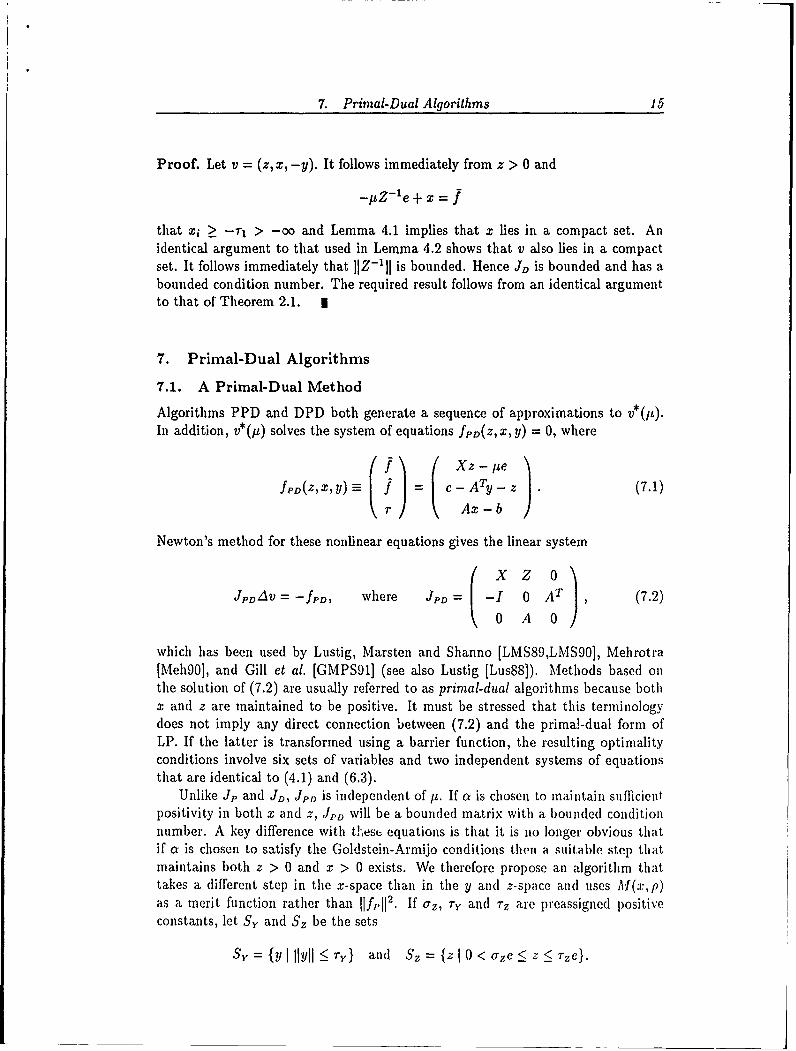
Algorithms PPD and DPD both generate a sequence of approximations to 1*(IL).In addition, v*(p) solves the system of equations fpD(Z,X, y) 0, where

f Xz - p

fPD(Z,X,y) = = c- ATy - z (7.1)r Ax - b

Newton's method for these nonlinear equations gives the linear system

JPDAv = -fPD, where JPD = -1 0 AT , (7.2)0 A 0

which has been used by Lustig, Marsten and Shanno [LMS89,LMS90], Mehrotra[MehgO], and Gill et al. [GMPS91] (see also Lustig [Lus88]). Methods based onthe solution of (7.2) are usually referred to as primal-dual algorithms because bothx and z are maintained to be positive. It must be stressed that this terminologydoes not imply any direct connection between (7.2) and the primal-dual form ofLP. If the latter is transformed using a barrier function, the resulting optimalityconditions involve six sets of variables and two independent systems of equationsthat are identical to (4.1) and (6.3).

Unlike Jp and JD, JPD is independent ofu1. If a is chosen to maintain sufficient

positivity in both x and z, JPD will be a bounded matrix with a bounded conditionnumber. A key difference with th.est- equations is that it is no longer obvious thatif a is chosen to satisfy the Goldstein-Armijo conditions then a suitable step thatmaintains both z > 0 and x > 0 exists. We therefore propose an algorithm thattakes a different step in the x-space than in the y and z-space and uses A'f(x,p)as a merit function rather than Ijfp[I2 . If oz, 7y and rz are preassigned positiveconstants, let Sy and Sz be the sets

Sy-{Y=fy lyllr and Sz={z1O<azez<rze}.


Algorithm PD (Model Primal-Dual Algorithm)

Set vo, with xo > 0, zo E Sz and yo E Sy;Set k = 0, i = 0 and ik = 0;while not converged do

Set ji = Ilk;while JINTg(xi,jz)jI + irl > ,k/' do

Select any zj+j E Sz and yi+j E Sy;Solve JPDAVi = -fpD for Axi;Find xj+1 = xi + aiAxi such thatM(xi+1,p) < M(xi,p) and xi+i > 0;Set i = i+ 1;

end do;Set k = k + 1, i k = i;

end do

The convergence of Algorithm PD follows directly if it can be shown that (7.2)generates a sequence {x} converging to x*(z).

Given positive constants Tr Ind TM, define the level set

9 = {x I IlAx - b!I 5r,, M(x,p) < 7"M}.

Similar arguments used to prove Lemma 4.1 show that S is compact.

Lemma 7.1. If x E S then there exists a positive ax, independent of x, such thatxi >_ axe. I

Lemma 7.2. Given positive constants r,, ry, rx and rz, assume that x, y and zsatisfy IlrIl = ljAx - bll - rr, Ilyll < ry, 0 < x < rxe and 0 < z < rze. Then thereexist constants p, y (y > 0) and / (/P > 1) such that

AxTVM(x,p) <_ -IIN~"ll 2 - 1i1rill,

where Ax is defined by (7.2).

Proof. If the system

(ZX - 1 A T ) AX) -( LX - l e b - (7.3)

is solved for Ax and Ay, it follows from the assumptions that IAxII is bounded.Observe that the right-hand side of (7.3) is identical to that of (2.2). It follows

thatINAxN = -NT(g + ZX-'ATAxA), (7.4)

where g = VB(xIt), HN = NTZX-lN, Ax = NAXN + ATAXA, and

AATAxA = -r. (7.5)

7. Primal-Dual Algorithms 17

Consider now the merit function M(x,p) given in Section 3. By definition wehave

AxTVM(x,p) = AXTNT(g + pATE) + AxT A(g + pATE),

where E is a vector whose elements are one in magnitude and whose signs are thesame as r. Define u =_ (AAT)- 1 A(I - X-1ZNII-lNT)g. Substituting for AxNfrom (7.4) and Axa from (7.5) gives

AxTVM(x, p) = -gTNH'lNTg - rTu - prTE,

_< -IIIN Tg2 -/311r11i,

where -' > 0 is the reciprocal of the largest eigenvalue of 11N,/3 _ 1, and p is chosensuch that

p = max(1 - rTuM, 0),rTE

with um the vector u evaluated at the point x E S for which rTu has its minimumvalue. I

Lemma 7.3. If Ax is defined by (7.2), there exist positive a and ax such that the

Goldstein-Armijo conditions are satisfied with x + aAx > axe.

Proof. If aM is the largest feasible step along Ax, then M(x + aMAx, p) is infinite

and it follows that there exists a positive number a* that solves the problem ofminc, M(x + aAx, p) subject to x + aAx > 0. Hence, a strictly feasible point existsfor which the Goldstein-Armijo conditions are satisfied. I

Lemma 7.4. Let az, r, and r7 be preassigned positive constants. Consider sc-qunces {zi} and {yi} such that aze < zi < rze and HYill < r. Let {xi} denote

the sequence x,+, = xi + a, Ax, and xo > 0, where Ax, is defined by (7.1) andai satisfies the Goldstein-Armijo conditions on M(x,p) with the requirement thaixi+l > 0. If p is sufficiently large (but bounded) then limi-.. xi = x*().

Proof. Since {xi} lies in a compact set, it follows that x, is bounded for all i.Moreover, since xi lies in S, there exists a positive ax such that x, > axe for all i.Every element of the sequence {x,} satisfies the assumptions of Lemma 7.2 and wehave

Ax7'1AM(xi,p) _ -711JNTg(xi)ll 2 - 0]lr(x,)ll,,

where -y > 0 and 3 _> 1. It follows from Lemma 7.2 that {M(x,,p)} is a strictly

monotonically decreasing sequence. Since {x,} E 5, it follows that {AI(x,,p)} miul.1converge and the Goldstein-Armijo conditions give

lim aiAX7 VM(xi,p) = Jim ai(-yJJN7g(x,)Il2 + 0I1r(x,)I 1) = 0.1T00 t 00

Trhe proof now follows a similar argument to that given in Lemmna 2. 1.

S

$' 18 Primal-dual methods for linear programming

Lemma 7.5. If the assumptions and definitions of Lemma 7.4 hold then

Jim yi + Ayi = Y*(p) and lim zi + Azi = z*(p).t--o i--o

Proof. It follows from (7.3) and the optimality conditions of (2.1) that

lim yj + Ayi = y*() and lim Axi = 0.l-.-00 i---00

From (7.2) we have Zi(xi + Axi) = -XiAzi + tie. Since limi-..o xi = x*(jI) andlim-. 00 Axi = 0, we have

lim zi + Azi = IzX*()-le = z*(j,),

where X*(u) = diag((x*(1i))). I

The above result shows that even for quite arbitrary choices of {zi} and {yij,approximations to y*(p) and z*(yi) may be obtained.

In practice, certain choices of zi and yi lead to more efficient algorithms. Theprimal algorithm of Section 3.2 using the merit function M(x,p) may be viewed asbeing equivalent to Algorithm PD with zi chosen as IiXrle and yi+l = yi + aiAyi.Since IIAx - bill is implicitly bounded by the linesearch, Lemma 4.1 implies that xiis bounded. It follows that each (zi)j is bounded away from zero, and zi E Sz forsuitably small az.

Alternatively, values of y and z may be determined from a linesearch. A steplength0, in the z and y-space can be taken as an approximate solution of the univariateproblem

minimize IIfPD(Zi + OAzi, Xi, Y, + OAyi)II2

e

subject to zi + OAzi > rllX4+\e, 0 < 1,

where 7 is some preassigned constant in (0, 1].

7.2. Another Primal-Dual Algorithm

A second primal-dual algorithm can be derived by observing that v*(Il) solves thesystem of equations fPDD(z,x,y) = 0, where

f oo (Z, X,Y) = c - Ary - z (7.6)r Ax - b

Newton's method for these equations gives the linear syctem JPDDAV = -fPDD,

where

JPDD = -I 0 AT

0 A 0

8. The Treatment of Free Variables i9

Unlike the primal-dual method of Section 7.1, there always exists a steplength thatsatisfies both the Goldstein-Armijo conditions for IIfPDD 112 and the restrictions x +acAx > 0 and z + aAz > 0.

The proof of the following theorem is similar to that of Theorem 6.1.

Theorem 7.1. Let {vi} be the sequence generated by Newton's method applied tothe equations (7.6). Then limi.. Ilvi - v*(Is)ll = 0. 1

At first sight, the Jac-' ian JPDD looks more complicated than JPD. Ilowevr,

the KKT matrix for the system is identical to that for the primal-dual method ofSection 7.1. We have

/ 12ZX-1 AT 'dX c-2z+IZ x - ATY 7.7= -y) (7.7)A ) ( - ,:Ay A x - b

Herce, the search direction for the PD algorithm of Section 7.1 may be computedwith little additional effort. A better direction can perhaps be constructed from thetwo search directions. The precise combination can be made dynamic and need bespecified only after both directions are known.

The right-hand side of (7.7) is identical to the right-hand side for the KKT systemof the dual algorithm. This implies that this algorithm is related to the dual barrieralgorithm in the same way that the primal-dual algorithm of Section 7.1 is relatedto the primal. For example, a merit function based on the dual barrier functionand dual constraint violations would enable the calculation of different steps in theprimal and dual variables. In this case it is the step in the primal variables thatmay be chosen arbitrarily.

Note that any linear combination of the systems of equations (7.6), (7.1), (4.1)and (6.3) also leads to a similar algorithm. In particular, any linear Combinationthat includes the primal-dual equations (7.6) (no matter how tiny a proportion) hasthe property that a suitable steplength exists for which x and z are positive.

8. The Treatment of Free Variables

If there are no bounds on a particular variable, no difficulty arises provided zAvis computed directly from the KKT system. However, a common approach for(oinputing Av is first to compute Ay using the Schur complement of the leadingdiagonal matrix. If the leading diagonal '. singular, such an approach cannot beused. (We may always use the Schur complement of the nonjingular portion of thediagonal matrix but this is no longer a definite system.)

We shall consider just the primal algorithm, but the approach suggested heremay be used in all the methods. For simplicity, assume that x, is the only freevariable. In place of (f1), = z, -- ltIxr we now have (fp)r = Zr, with z(tt) = 0. As

long as the explicit KKT system is solved, the effect of this equation on the Jacobianis inconseluential. tlowever, in place of jiX - 2 we now have D, where d, = 0 anddj = tx for j 0 r. Hence D is singular and its Schur complement does not exist.


A means of circumventing this difficulty is to replace the equation zr = 0 by anequation that ensures zr -+ 0 as it -- 0. For example, we could use

eXrzr = / or Zr +PXr = 0,

which give dr = Zr and dr = I respectively. In the first example, z*(4t) = Ile

and we may keep zr > a, > 0. It follows that D is nonsingular and its Schurcomplement exists. In the second example, since zr does not appear in the Jacobian,its sign or magnitude is not important. Likewise, the nonsingularity of Jp no longerdepends on x,, so there is no need to restrict the steplength for this variable.

9. Further Comments

A common practice in interior-point implementations is to define the steplength assome fixed percentage of the maximum feasible step. By contrast, all the algorithmsdescribed in this paper require some form of linesearch for the steplength. In practicethis requirement has a minimal effect upon computation time, given the work neededto compute the search direction. Moreover, if r is close to one and n is close tozero, almost any step is likely to satisfy the Goldstein-Armijo conditions because allthe linesearch functions are convex and increase rapidly near the boundary of thefeasible region. In practice we have observed that the need to perform a linesearcharises, aly when there is significant numerical error in the search drection.

Currently the most efficient implementations use a predictor-corrector methodto define the search direction (e.g. [LMS90,Meh90]). Such a strategy may be incor-porated in the algorithms discussed here. The important point is to be able to fallback on a guaranteed method should the predictor-corrector direction fail to be asuitable descent direction for the merit function. A similar view was adopted byMehrotra [Meh90].

It has not been our intent to compare the various algorithms in terms of perfor-mance. All the primal-dual algorithms have very similar theoretical properties, butonly the primal-dual algorithm of Section 7.1 has been used in the principal knownimplementations [LMS89,LMS90,Meh9O,GMPS91]. The key system of equations is"less nonlinear" than for the other three variations. Even so, in the neighborhood ofthe solution, the Jacobian behaves almost identically to the Jacobians of tile othersystems (as does the KKT matrix). It is not immediately apparent that this methodis inherently superior to the others.

It may be that the best method is dependent on how the linear systems aresolved. For example, all the methods may be implemented by solving systems ofthe form ADATdy = u, where D is either X 2, Z - 2 or XZ "'l . Suppose thesesystems are solved using a conjugate gradient method in which a preconditioner isbased on periodically forming the Cholesky factors of ADAT. The systems usingD = X 2 should yield better preconditioners as the iterates converge because theratio of consecutive values of any significant diagonal of D converges to one. WhenD = XZ - ' or D = Z - 2 , the significant diagonals correspond to the small elementsof z. It is not obvious that the ratio of consecutive values of any such diagonal willbehave as smoothly.

References 21

Our analysis is directed at the linear programming problem. However, extendingthe results to a smooth convex objective function is quite straightforward. The morechallenging problem is to extend the results to nonconvex problems.

Acknowledgement

The authors are grateful to Joe Shinnerl for his careful reading of the manuscriptand a number of helpful suggestions.

References

[FM68] A. V. Fiacco and G. P. McCormick (1968). Nonlinear Programming: Sequential Un-constrained Minimization Techniques, John Wiley and Sons, New York and Toronto.

[GMSTW86] P. E. Gill, W. Murray, M. A. Saunders, J. A. Tomlin and M. It. Wright (1986).On projected Newton barrier methods for linear programming and an equivalence toKarmarkar's projective method, Mathematical Programming 36, 183-209.

[GMPS91] P. E. Gill, W. Murray, D. B. Poncele6n and M. A. Saunders (1991). Solving reducedKKT systems in barrier methods for linear and quadratic programming, Report SOL91-7, Department of Operations Research, Stanford University.

[KMY89] M. Kojima, S. Mizuno and A. Yoshise (1989). A primal-dual interior-point algorithmfor linear programming, in N. Megiddo (ed.), Progress in Mathematical Programming,Springer-Verlag, New York, 29-47.

(KMM90] M. Kojima, N. Megiddo and S. Mizuno (1990). Theoretical convergence of large-step primal-dual interior-point algorithms for linear programming, Report RJ 7872(72532), IBM Almaden Research Center, San Jose, CA.

[Lus88] I. J. Lustig (1988). Feasibility issues in an interior-point method for linear program-ming, Report SOR 88-9, Department of Civil Engineering and Operations Research,Princeton University, Princeton, NJ.

[LMS89] I. J. Lustig, R. E. Marsten and D. F. Shanno (1989). Computational experiencewith a primal-dual interior-point method for linear programming, Report SOR 89-17, Department of Civil Engineering and Operations Research, Princeton Univelsity,Princeton, NJ.

[LMS90] I. J. Lustig, R. E. Marsten and D. F. Shanno (1990). On implementing Mehrotra'spredictor-corrector interior-point method for linear programming, Report SOR 90-3, Department of Civil Engineering and Operations Research, Princeton University,Princeton, NJ.

[MMS89] K. A. McShane, C. L. Monma and D. F. Shanno (1989). An implementation of aprimal-dual interior-point method for linear programming, ORSA Journal on Com-puting 1.

[Meg89] N. Megiddo (1986). Pathways to the optimal set in linear programming, in N. Megiddo(ed.), Progress in Mathematical Programming, Springer-Verlag, New York, 131-158.

(Meh90] S. Mehrotra (1990). On the implementation of a primal-dual interior-point method,Report 90-03, Department of Industrial Engineering and Management Sciences.Northwestern University, Evanston, IL.

[MA89] R. D. C. Monteiro and I. Adler (1989). Interior path-following primal-dual algorithnms,Part 1: Linear programming, Mathematical Programming 44, 27-41.

[OR70] J. M. Ortega and W. C. Rheinboldt (1970). Iterative Solution of Nonhnear Equattonsin Several Variables, Academic Press, London and New York.

[Pon90] D. B. Poncele6n (1990). Barrier methods for large-scale quadratic programmig, P11.l).Thesis, Computer Science Department, Stanford University, Stan ford.

REPORT DOCUMENTATION PAGE [ FM orm 0704.0

#.a rolnit buro for tr,,, (0iwon~O of info-malien 9 "tout" toVoe I Aw IW l 'ACIU6Nq tAO tt tI rwr m-." 1"r'fumtoms nstcPWlq 0@0tons A U wIqatA~~q *g mO the 19 4. WW o"an CON0"tAl a NV*WIA the 1gI9.d.OA of ,AtoWmaBoIoI9 b common% to?.t.AI tits burg"t onim.to or o"r It199.& of~S thmq

=oteb f Inor" ,anyOt.0f "0lt.A W torts fo nowiniii thts boAo to WIIA.AqIOA W ds" ift $"vicel 061,000 10 @1 t010G-f OW tSIM n Roer 121 fl oron~9SOan,,.1P~~~~~~~~wh,~~ lu'll I~4&leg@ voonV Alpliit~~~lse$ e~qmetuasah pow 10gl.A9I 7 O1S) woompWn C 1S

1. AGENCY USE ONLY (LeAVe 641 1k) 1. REPORT DATE 3.REPORT TYPE AND DATES COVEREDMay 1991 Technical Report

4. TITLE AND SUBTITLE S. FUNDING NUMBERS

Primal-Dual Methods for Linear Programming NOOl14-90-J-1242

6. AUTHOR(S)

Philip E. Gill, Walter Murray, Dulce B. Poncele6nand Michael A. Saunders

7. PERFORMING ORGANIZATION NAME(S) AND ADDRESS(ES) 8. PERFORMING ORGANIZATIONREPORT NUMBER

Department of Operations Research - SOLStanford UniversityStanford, CA 94305-4022 1111 MA

9. SPONSORING MONITORING AGENCY NAME(S) AND ADDRESS(ES) 10. SPONSORING / MONITORING

Office of Naval Research - Department of the Navy AGENCY REPORT NUMBER

300 W. Quincy StreetArlington, VA 22217 SQL 91-3

12a. OIST~ki5 1 TsOh~ AVAILABILITY STATEMENT 12b DISTRIBUTION CODE

UNLIMITED UL

13. ABSTRACT (Maxiurn200 wocu)

Many interior-point methods for linear programming are based on the properties of the logarithmicbarrier function. We first give a convergence proof for the (primal) projected Newton barrier methodWe then analyze three types of barrier method that can be categorized as primal, dual and primal-dualAll three approaches may be derived from the application of Newton's method to different varants of thcsame system of nonlinear equations. A fourth variant of the same equations leads to a new primal-dualalgorithm.

In each of the methods discussed, convergence is demonstrated without the need for a nondlegen-eracy assumption In particular, convergence is established for a primal-dual algorithm that allows adifferent step in the primal and dual variables

Finally, we describe a new method for treating free variables.

14. SUBJECT TERMS 1S. NUMBER OF PAGES

linear programming; barrier methods, interior-point methods. 21 D~aaes16. PRICE CODE

17. SECU.RITY CLASSIFICATION 18. SECURITY CLASSIFICATION 19 SECURITY CLASSIFICATION 20. LIMITATION OF ABSTR-ACTOF REPORT OF THIS PAGE OF ABSTRACT

UNCLASSI FIED I SAR

!.. CfC - -*.k

418 syptems dtic · initially we prove convergence for a primal barrier algorithm in which the...

Documents