401(k) plan participant retirement income security: plan ... meetings/1b-401.pdf ·...

Preliminary—Please do not cite or quote without the author’s permission

401(k) Plan Participant Retirement Income Security: Plan Sponsors’ Selection of Target-Date Funds and Automatic Contribution Arrangements

Youngkyun Parka

Current version: July 2012

Submitted for the 2012 ARIA conference

Abstract

Given a wide variety of target-date fund equity glide paths, this paper investigates the potential variation in 401(k) plan participant retirement income security that can result from a plan sponsor’s selection, and identifies ways to lessen the potential for variation with simulations based on empirical findings on participant contributions to 401(k) plans. Drawing on research on financial literacy and peer effect, participant demographic characteristics at plan level (“plan demographics”) are considered as influencing participant saving behavior for retirement. Using a large sample of 401(k) plans (with over 485,000 participants in 674 plans), plan demographics are shown to have a significant effect on participant contribution rates. Simulations results by plan demographics indicate that the potential for variation in the retirement income security of plan participants can be reduced with the adoption of a customized automatic contribution arrangement that reflects the plan demographics. Keywords: Automatic contribution arrangement Plan demographics Retirement income security Target-date funds 401(k) plans a College of Business and Economics, University of Idaho, contact: [email protected]

1

1. Introduction

The Securities and Exchange Commission (SEC) addresses in its proposed rule that

“market losses incurred in 2008, coupled with the increasing significance of target date funds in

401(k) plans, have given rise to a number of concerns about target date funds (75 FR 35921)”.1

In particular, plan sponsors as a fiduciary, are concerned about their selection of target-date

funds as a default investment option when the funds underperform relative to their Investment

Policy Statement (IPS) standards (PLANSPONSOR, 2008).2 The Pension Protection Act of 2006

(PPA) provisions provide fiduciary responsibility relief for plan sponsors when they satisfy

certain rules. However, the provisions do not relieve all fiduciary obligations, and plan sponsors

should still meet general fiduciary responsibility (72 FR 60453).3 This paper investigates the

potential variation in 401(k) plan participant retirement income security that can result from a

plan sponsor’s selection of target-date funds and identifies how the potential for variation can be

1 Securities and Exchange Commission’s Proposed Rule, “Investment Company Advertising: Target Date Retirement Fund Names and Marketing (17 CFR Parts 230 and 270),” Federal Register on June 23, 2010 (75 FR 35921). 2 Although the SEC did not mention plan sponsors’ concerns about the selection of target-date funds as a default investment option in its proposed rule (75 FR 35921), their concerns are well addressed in the results of the PLANSPONSOR 2008 Survey: about 66.7% of the 5,973 plan sponsors surveyed indicated that they were at least somewhat concerned about litigation resulting from auto-enrolling participants into target-date funds that did not meet their IPS standards. An IPS provides guidelines for a fiduciary to make investment decisions and monitor, and once a plan sponsor sets an IPS, the plan sponsor should comply with it; otherwise, this may serve as evidence of a fiduciary’s imprudence (AllianceBerstein, 2010). The PLANSPONSOR magazine has conducted annual surveys of the defined contribution plan sponsors. For the 2008 Survey, the PLANSPONSOR sent out surveys in July and August 2008 to approximately 35,136 and collected qualifying results from 5,973 respondents by September 10, 2008 (PLANSONSOR, 2008). 3 When plan sponsors adopt target-date funds as a qualified default investment alternative (QDIA), the PPA provides protection from fiduciary liability from losses when a plan sponsor selects investments for plan participants who have not made their own investment decisions (see “Default Investment Alternatives Under Participant Directed Individual Account Plans (29 CFR Part 2550),” Federal Register on October 24, 2007 (72 FR 60452)). However, plan sponsors still must satisfy general fiduciary duties of prudence and loyalty when selecting and monitoring any target-date funds. Therefore, plan sponsors should reflect these duties in selecting a particular target-date fund (72 FR 60453).

2

lessened when the plan sponsor auto-enrolls participants in target-date funds as a default

investment vehicle.4

Target-date funds (TDFs, also known as “lifecycle funds”) have gained popularity as a

default investment option in company-sponsored defined contribution plans, such as 401(k)

plans, since the PPA and its subsequent regulations were established.5 At the same time,

however, TDFs showed a wide variation in returns (even those with the same target date), in

particular in 2008 and 2009. According to the 2010 Morningstar Industry Survey, annual returns

for 2010 TDFs ranged from a loss of 41.3% to a loss of 9.1% in 2008, whereas the returns for the

2010 funds ranged from gains of 7.3% to 30.8% in 2009 (Charlson, Falkof, Herbst, Lutton, and

Rekenthaler, 2010).

The wide variation in TDF performance results mainly from a variety of equity glide

paths of the funds (SEC, 2010). TDF providers (also referred to as TDF families) offer the funds

based on their unique equity glide paths (Charlson et al., 2009).6 TDF families provide a wide

variety of equity glide paths (see Figure 1), and the heterogeneity of these glide paths has

increased since the PPA was enacted in 2006 (Balduzzi and Reuter, 2012).7 Since 401(k) plan

sponsors tend to select TDFs from a single fund provider (GAO, 2011), plan sponsors are likely

4 In the paper, a 401(k) plan sponsor refers to a company that sponsors 401(k) plans. A company sponsors a single or multiple 401(k) plans. 5 A target-date fund (TDF) is designated as a qualified default investment alternative (QDIA) along with a “balanced fund” or professionally “managed account” by the Department of Labor regulations pursuant to the PPA (see “Default Investment Alternatives Under Participant Directed Individual Account Plans (29 CFR Part 2550),” Federal Register on October 24, 2007 (72 FR 60452)). The PPA provides fiduciary responsibility relief when a plan sponsor adopts a QDIA. Among QDIAs, TDFs have become popular in defined contribution plans. For example, Fidelity Investments (2009), one of the largest 401(k) plan administrators, reports that 62% of the plans administered by the company used TDFs as a default investment option as of March 2009, up from 5% at the end of 2005. 6 Target-date funds, unlike other balanced funds, have a unique common feature: a pre-determined declining equity exposure as the investor approaches the target date. The shift in equity allocations is often referred to as an “equity glide path.” 7 Figure 1 illustrates the wide variety of equity glide paths offered by TDF providers. For example, for the 2010 funds in 2009, the difference in equity allocations across the funds reached as much as about 40 percentage points.

3

to be concerned about their selection of fund providers while observing the wide variation in

TDF returns.8

Responding to the wide variation in TDF performance, plan sponsors as a fiduciary—in

particular, those who auto-enroll participants in TDFs—may consider two options to increase the

retirement income security of the plan participants. One option is to replace the TDF provider

with another: namely, one that provides more appropriate equity glide paths for the plan

participants (GAO, 2011). However, this option would lead to a high opportunity cost. Given

that most TDF providers will also play the role of record keeper, any switching between TDF

providers can incur substantial conversion costs: these may include costs that arise from changes

to computer systems and record-keeping and payroll processes and converting account balances

(GAO, 2011).9

The other option is to raise participant contribution rates by modifying the automatic

employee contribution arrangement, which includes a default employee contribution rate (as a

percentage of compensation) and a maximum level of automatic contribution increases

(VanDerhei and Lucas, 2010). This option would have a low opportunity cost, because it draws

little resistance from plan participants. For example, most participants tend to accept a high

default contribution rate (Fidelity Investments, 2009) and a high level of automatic contribution

escalation (VanDerhei, 2007). Therefore, the option using an automatic employee contribution

arrangement may be more attractive to the 401(k) plan sponsors who auto-enroll participants in

TDFs.

8 GAO (2011) reports the reliance of plan sponsors on their record keeper TDFs by citing the BrightScope’s analysis that in 2009, 96 percent of 401(k) plans with TDFs that were clients of the largest record keepers use the record keeper’s proprietary TDFs. 9 A record keeper provides record-keeping services such as plan administration, monitoring of plan participant and beneficiary transactions (e.g., enrollment, payroll deductions and contributions, loans, withdrawals, and distributions), and the maintenance of plan accounts and statements (GAO, 2011).

4

To ensure that an automatic contribution arrangement is effective for the retirement

income security of plan participants, plan sponsors should understand the factors that influence

the contribution behavior of plan participants. Many studies on 401(k) plans find that

participants’ saving behavior is significantly affected by plan design features (such as automatic

enrollment default contribution rate, automatic contribution escalation, employer matching, loan

provisions, and investment options).10 However, few studies pay attention to participant

demographic characteristics at plan level (known as “plan demographics”), which would be

related to peer effect in retirement savings decisions within a plan. Research on financial literacy

and peer effect suggests that plan demographics influence participant saving behavior for

retirement in a plan. For example, those with a low income are likely to be less financially

literate and less interested in retirement (Hogarth and Hilgert, 2002; Hilgert, Hogarth, and

Beverly, 2003; Gustman and Steinmeier, 2005; Lusardi and Mitchell, 2007, 2010). In particular,

when a participant is in a plan that includes a large group of low-income employees (this is one

of the plan demographics), the participant is likely to have a lower contribution rate than

otherwise because of peer effect (Duflo and Saez, 2002, 2003). Therefore, as long as plan

demographics are related to the contribution behavior of plan participants, the plan sponsor needs

to consider plan demographics as well as plan features when designing an automatic contribution

arrangement to enhance participants’ retirement income security.

10 For example, Choi, Laibson, Madrian, and Metrick (2004b) and Madrian and Shea (2001) report strong effects of automatic enrollment on participant contribution rates, and Benartzi and Thaler (2004) find a significant influence of automatic contribution escalation on contribution rates. Clark and Schieber (1998), Cunningham and Engelhardt (2002), Huberman, Iyengar, and Jiang (2007), and Papke and Poterba (1995) document positive effects of employer matching on contribution rates. As for loan provisions, GAO (1997), Holden and VanDerhei (2001), Mitchell, Utkus, and Yang (2007), and Munnell, Sunden, and Taylor (2002) report positive effects on contribution rates. Papke (2004) finds that the ability to exercise choice over investment allocations increases contribution rates. Last, when company stock is an investable fund, Huberman et al. (2007) report its significant influence on participant contribution rates.

5

This paper outlines empirical evidence that plan demographics (defined by participant

income and/or tenure) are significantly related to participant contribution rates. This evidence is

obtained using a large sample (over 485,000 participants in 674 plans) from the 2007 Employee

Benefit Research Institute (EBRI)/Investment Company Institute (ICI) 401(k) database, one of

the largest 401(k) plan databases in the United States.11 In addition, simulations based on the

empirical findings by plan demographics show that the potential variation of the plan

participants’ retirement income security that occurs as a result of a plan sponsor’s selection of

TDFs (i.e., a TDF equity glide path) can be reduced by adopting a customized automatic

contribution arrangement that reflects the relevant plan demographics.

This paper extends previous research in three directions. First, this paper addresses plan

sponsors’ concerns (as a fiduciary) about TDF adoptions in 401(k) plans in relation to plan

participants’ retirement income security. Earlier studies, in contrast, focus on the evaluation of

TDFs (or life-cycle investment strategies) in retirement plans from the perspective of individual

investors (e.g., Bodie and Treussard, 2007; Gomes, Kotliko, and Viceira, 2008; Poterba, Rauh,

Venti, Wise, 2009; Viceira, 2009; Basu, Byrne, and Drew, 2011). Given that plan participants’

TDF choices are usually constrained by the plan sponsor’s selection of TDFs, plan participants’

retirement income security needs to be examined with the plan sponsors’ TDF selections.

Second, this paper adds to the literature on 401(k) plan participants’ saving behavior, by

showing that plan demographics are associated with individual contribution rates. This finding

can serve as evidence for peer influence in retirement savings/investment decisions within a plan

(e.g., Duflo and Saez, 2002, 2003; Lu, 2011).

11 The 2007 EBRI/ICI database includes 21.8 million participants in 56,232 401(k) plans, covering 45% of the estimated universe of active 401(k) plan participants and 12% of all 401(k) plans (VanDerhei, Holden, Alonso, and Copeland, 2008).

6

Third, this paper contributes to the literature on automatic features in 401(k) plans (e.g.,

Madrian and Shea, 2001; Benartzi and Thaler, 2004; Choi, Laibson, Madrian, and Metrick,

2004b; VanDerhei and Lucas, 2010) by showing that the effects of automatic features on

retirement income adequacy differ according to plan demographics. In addition, this finding

provides 401(k) plan sponsors an insight into an effective automatic contribution arrangement for

participant retirement income security: that an automatic contribution arrangement should be

designed by taking into account different participant contribution behavior by plan

demographics.

The remainder of the paper is organized as follows. The next section addresses

institutional background on automatic enrollment under the PPA. Section 3 discusses plan

demographics that influence participant contribution behavior. Section 4 provides empirical

findings on different participant contribution rates by plan demographics. Section 5 presents

simulation results indicating different effects of automatic contribution arrangements on

participant retirement income adequacy by plan demographics. Section 6 concludes the paper.

2. Automatic enrollment under the Pension Protection Act of 2006

Since the PPA was enacted in 2006, plan sponsors have increasingly adopted automatic

enrollment programs. For example, Fidelity Investments (2011) reports that 21% of the plan

sponsors that are administered by the company offer automatic enrollment as of 9/30/2011, up

from 2% as of 9/30/2006, six weeks after the passage of the PPA. Automatic enrollment has not

been a traditional feature of 401(k) plans.12 The PPA provisions, however, encourage plan

sponsors to automatically enroll employees in their 401(k) plans. For example, the PPA pre-

empts any state law that would directly or indirectly restrict the adoption of automatic enrollment 12 For more details on the automatic enrollment program prior to the PPA, see GAO (2009).

7

in a plan and provides a nondiscrimination safe harbor to plans that adopt an automatic

enrollment arrangement (GAO, 2009).

An automatic enrollment nondiscrimination safe harbor, in particular, is exempt from

required annual tests under sections 401(k)(3) and 401(m)(2) of the Internal Revenue Code

(IRC), which ensure that the plan does not discriminate in favor of highly compensated

employees (see IRC sections 401(k)(13) and 401(m)(12)).13 To qualify for the nondiscrimination

safe harbor, however, the plan must provide additional plan features to automatic enrollment,

such as a qualified automatic contribution arrangement (QACA) and a qualified default

investment alternative (QDIA).

A QACA includes two key components: automatic employee contributions and employer

matching contribution (or employer non-elective contribution), each of which should provide the

following automatic contribution arrangements. For employee contributions, the plan has (1) to

defer at least 3% of compensation in the first year (also referred to as a default contribution rate)

and (2) to automatically increase employee contribution by 1% each following year, to a

minimum of 6% and to a maximum of 10% of compensation. As for employer contributions, the

plan must match 100% of the first 1% of employee contributions and 50% of the next 5% of

employee contributions, up to 6% of compensation (or an employer non-elective contribution

equal to at least 3% of compensation).14 When a plan meets the QACA requirements, the plan is

deemed to satisfy the annual actual deferral percentage (ADP) test under IRC section 401(k)(3)

and the actual contribution percentage (ACP) test under IRC section 401(m)(2), as well as the

top-heavy rules under IRC section 416 (IRS, 2007).

13 IRC sections 401(k)(13) and 401(m)(12) of IRC state that a plan that meets certain requirements (e.g., automatic employee contributions at a specified level, employer matching contribution, uniformity, and notice requirement) is treated as satisfying required annual tests described in sections 401(k)(3) and 401(m)(2). 14 See “Automatic Contribution Arrangements (26 CFR Parts 1 and 54),” Federal Register on February 24, 2009 (74 FR 8200).

8

In addition, the plan must offer an investment vehicle which is designated as a QDIA by

the Department of Labor regulations under the PPA. A QDIA includes three investment options:

a target-date fund, a “balanced fund,” or a professionally “managed account,” each of which

provides fiduciary responsibility relief. Among the three investment options, TDFs have become

overwhelmingly popular in 401(k) plans with automatic enrollment. For example, according to

GAO (2009), Fidelity Investments reports that 96% of the plans offering automatic enrollment

used TDFs as a default investment option as of March 2009, up from 57% at the end of 2005.15

When plan sponsors adopt TDFs as a QDIA, the PPA provides fiduciary responsibility relief, as

mentioned above. However, not all fiduciary responsibilities are relieved. In particular, when

plan sponsors have an investment policy statement (IPS) about TDFs, they should monitor their

TDF selection to ensure that the TDFs meet the standards set by their IPS. An IPS provides

guidelines for a fiduciary to make investment decisions and monitor, and once a plan sponsor has

an IPS, the plan sponsor should adhere to it; otherwise, this may serve as evidence of a

fiduciary’s imprudence or even provide the basis for a claim against the fiduciary

(AllianceBerstein, 2010).

This paper focuses on plan sponsors that use an automatic enrollment nondiscrimination

safe harbor— in specific, those who adopt TDFs as a QDIA and seek an effective QACA to

enhance the plan participants’ retirement income security.

3. Plan demographics and plan participants’ saving behavior for retirement

To establish an effective qualified automatic contribution arrangement (QACA) for the

plan participants’ retirement income security, plan sponsors should identify the factors that affect

15 Another large 401(k) plan administrator, Vanguard Group (2011), also reports an increase in the popularity of TDFs as a default investment option for 401(k) plans offering automatic enrollment: in 2010, 92% of the plans with automatic enrollment policies adopted TDFs as a default fund, up from 42% in 2005.

9

the plan participants’ saving behavior. Previous studies have documented that plan design

features (e.g., employer matching, loan provisions, investment options in the plan, and automatic

enrollment) significantly influence the plan participants’ savings for retirement, controlling for

participant demographics. First, employer matching has a positive effect on participant

contributions (e.g., Clark and Schieber, 1998; Engelhardt and Kumar, 2007; Huberman, Iyengar,

and Jiang, 2007), although some studies report limited or negative effects on participant

contribution rates (e.g, Papke, 1995; Papke and Poterba, 1995; Kusko et al, 1998; Mitchell,

Utkus, and Yang, 2007). Second, loan provisions (which can relax liquidity constraints of the

plan participants) have a positive effect on participant contributions (e.g., GAO, 1997; Holden

and VanDerhei, 2001; Munnell, Sunden, and Taylor, 2002; Mitchell et al, 2007). Third, the

ability to exercise choice over investment allocations is likely to increase employee contributions

(Papke, 2004), but an increase in the number of fund options could negatively affect employee

contribution rates (as a percentage of compensation) (Huberman et al., 2007). Fourth, when

company stock is an investable fund in the plan menu, Huberman et al. (2007) report a positive

effect on participant contribution of low-income employees due to a “familiarity effect

(Huberman, 2001)”, although the significant effect is not found in other income categories.

Finally, regarding automatic enrollment (including default employee contribution rates and

automatic contribution escalation), Madrian and Shea (2001), Choi et al. (2004b), and Beshears

et al. (2008a) find that employee contribution rates tend to be anchored on the plan default

contribution rate, and Benartzi and Thaler (2004) document significantly positive effects of

automatic contribution escalation on employee contribution rates.

In addition to plan design features, plan demographics (i.e., participant demographic

characteristics at plan level) arguably influence participants’ savings for retirement. This

10

assertion is based on the findings in the literature on financial literacy, consumption-saving, and

peer effects. Two demographic characteristics are considered: plan participants’ income and

expected job tenure in the current plan. First, plan participants’ income at plan level would affect

individual participant contribution rates. For example, participants with low income are likely to

lack both financial literacy and desire to save for retirement, and this leads to a low saving rate

for retirement (e.g., Hogarth and Hilgert, 2002; Hilgert et al., 2003; Gustman and Steinmeier,

2005; Lusardi and Mitchell, 2007, 2010). Further, when these participants consist of a large

group of a plan (indicating the plan demographic characteristics), a participant in the plan would

be likely to have a lower contribution rate than otherwise because of peer effect: individual

saving behavior for retirement is influenced by the contribution choices of colleagues (Duflo and

Saez, 2002, 2003).

Second, the expected job tenure of plan participants at plan level would affect individual

participant saving rates for retirement. Retirement saving behavior is related to the length of

financial planning horizon (Munnell et al., 2002; Ameriks et al., 2003; Reis, 2006). For example,

those with a short planning horizon are likely to have low employee contribution rates (Munnell

et al., 2002). A group of people have a short planning horizon because they want to reduce

sizable financial planning costs in an uncertain environment (Lusardi, 2003; Reis, 2006;

Caliendo and Aadland, 2007).16 Under the circumstances, participants with short expected job

tenure are likely to face high costs of planning and, thus, have a short planning horizon and a low

contribution rate. Similar to the plan demographics based on plan participants’ income, a

participant in a plan that has a large group of those with short expected job tenure in the current

16 Financial planning cost indicates the opportunity cost of taking the time to make saving plans (Reis, 2006). It can be interpreted as “the cost in money and time of obtaining information, processing and interpreting it, and deciding how to optimally act … [or] paying a financial advisor to interpret the information and compute the optimal financial plan (Reis, 2006, p. 1764).”

11

plan (indicating the plan demographic characteristics) would be likely to have a lower

contribution rate than otherwise due to the peer effect.

Few studies, however, have examined a relationship between the plan demographics and

the contribution behavior of plan participants. Noting that aggregate individual characteristics at

plan level are associated with potential peer effect, Huberman et al. (2007) take into account

participant demographic characteristics at plan level. In their models, however, plan

demographics serve only as control variables (they use plan-level averages, such as average

compensation, average tenure, and average age). Plan demographics have not been considered in

the literature on automatic enrollment, either. Madrian and Shea (2001), Choi et al. (2004b), and

Beshears et al. (2008a) document well the effects of default employee contribution rates with

automatic enrollment on participant contributions, but they are unable to consider plan

demographics because they examine only a small number of case firms. In a simulation study on

automatic enrollment, VanDerhei and Lucas (2010) explore the impacts of auto-enrollment and

automatic contribution escalation on retirement income adequacy with various scenarios, but

their models do not consider plan demographics.

This paper, however, examines the effects of plan demographics on individual

contribution behavior, controlling for individual-level characteristics and plan feature variables.

Plan demographics are defined by considering two factors: plan participants’ income and actual

job tenure (not the expected one) at plan level. Since it is difficult to directly measure the

expected job tenure in the current plan with administrative records, which the paper uses, actual

job tenure in the current plan is instead used.17 In specific, the characteristics of the job tenure

distribution in the current plan are used in determining whether the plan participants expect short

17 In addition, the EBRI/ICI data that this paper uses does not include the information on employment termination of plan participants. Thus, the expected job tenure in the current plan based on employment termination date is not able to be computed.

12

or long tenure in the current plan. For example, when a participant is in a plan that has a large

group of those with short (long) tenure, the participant would expect short (long) job tenure in

the current plan.

4. Participant contribution behavior by plan demographics

This section examines whether plan demographics are significantly related to individual

participant contribution rates by controlling for individual- and plan-level characteristics, using a

sample of the 2007 EBRI/ICI 401(k) database.

4.1. Plan classification by plan demographics

For an empirical analysis of the effects of plan demographics on participant contribution

rates, plans are classified based on the median income and/or tenure of the plan participants with

the following steps.18

First, tertiles are computed on the distributions of salary and tenure from a sample of

participants who are between age 20 and 75, have at least 1 year but fewer than or equal to 40

years of tenure in the current plan, and have a salary of between $2,500 and $500,000 in 2007

dollars. The sample consists of 1,497,014 participants in 958 plans.

Second, a plan is assigned to one of three groups by identifying a location of the plan

median income (tenure) in the tertiles of the distribution of income or tenure (see Table 1). For

example, a plan with the median income of less than or equal to $35,200 (the first tertile) is

assigned to a low-income plan group, while one with the median income of greater than $63,600

(the second tertile) is assigned to a high-income plan group. A plan in the low- (high-) income

plan group can be regarded as one dominated by those with low (high) income, because at least

half of the plan participants have less than or equal to the lower tertile income (greater than or 18 In the paper, tenure indicates the length of time in the current plan.

13

equal to the upper tertile income). This also applies to plan demographics based on plan

participants’ tenure. A plan in the short- (long-) tenure plan group can be regarded as one

dominated by those with short (long) tenure, because at least half of the plan participants have

less than or equal to the lower tertile tenure (longer than or equal to the upper tertile tenure). The

cutoff points for short or long tenure are 5.1 or 12.4 years, respectively (see Table 1).19

Last, plans are further classified into nine groups based on the income and tenure

classifications (see Table 1). Among the nine plan groups, three groups are focused: Group I

(low-income and short-tenure), Group V (middle-income and mid-tenure), and Group IX (high-

income and long-tenure), which have the most contrasting plan demographics.

[Insert Table 1 about here]

4.2. Sample construction

Next, a sample is constructed with plans and participants that have complete information

on employer contributions, employee contributions, and participant demographics including age,

tenure, and salary.20 In specific, the sample includes only the plans that have at least 25

participants and in which at least 75% of the plan participants are active.21 The plans should also

offer plan loans. This constraint is to see the effect, if any, of the amount of outstanding loan

balance on contribution rates. At participant level, the sample contains those who are age 20 to

75 and have 1 to 40 years of tenure in the current plan. In addition, the participants should have a

salary of between $25,000 and $100,000. The lower bound of $25,000 is to control for part-time

employees,22 and the upper bound of $100,000 is to control for highly compensated employees

19 In addition, it is notable that since tenure indicates the length of time in the current plan, a short- (long-) tenure plan may indicate one with high- (low-) turnover. For example, a plan that has a large group of those with short tenure may represent one with high turnover of the plan participants. 20 The EBRI/ICI database used in the paper does not include the information on gender. 21 Active participants refer to those who contribute to their retirement accounts. 22 According to the Current Population Survey 2008 Annual Social and Economic Supplement (“Table PINC-05. Work Experience in 2007--People 15 Years Old and Over by Total Money Earnings in 2007, Age, Race, Hispanic

14

(HCEs).23 As a result, the sample includes only non-highly compensated employees. In addition,

the participants should have a contribution rate greater than zero but less than or equal to 25% of

salary, which is to control for outliers in the distribution of participant contribution rate.24

Participant contribution rates appear to differ by plan demographics based on income and

tenure. Panels A and B in Table 2 present low contribution rates of participants in low-income or

short-tenure plans. For example, the mean employee contribution rate of the low-income plans is

5.03% of salary, which is 1.42 percentage points (2.41 percentage points) lower than that of the

middle-income (high-income) plans. Also, the mean employee contribution rate of the short-

tenure plans is 5.41% of salary, which is 0.65 percentage points (1.95 percentage points) lower

than that of the mid-tenure (long-tenure) plans. Further, among Group I (low-income and short-

tenure), V (middle-income and mid-tenure), and IX (high-income and long-tenure), the

difference in the mean contribution rate between the groups becomes greater. The mean

contribution rate of Group I is 4.43% of salary, which is 1.83 percentage points (3.36 percentage

points) lower than that of Group V (IX).


4.3. Model specification

To scrutinize the effects of plan demographics on participant contribution rates, however,

one should control for individual-level and plan-level characteristics. The literature on

participant contribution rates in 401(k) plans indicates that participant contribution rates in

401(k) plans are affected by individual demographics characteristics and plan design features

Origin, and Sex”), 85.3% of workers who earned less than $25,000 a year are part-time ones in 2007. Part-time workers indicate those who worked less than 35 hours a week. 23 Highly compensated employees (HCEs) in 2007 are defined as those who earned greater than $100,000 (see Section 414(q)(1)(B) of the Internal Revenue Code). 24 The cutoff contribution rate of 25% corresponds to the 98.1th percentile of the distribution of participant contribution rate as a percentage of salary.

15

(e.g., Holden and VanDerhei, 2001; Huberman et al., 2007, Mitchell et al., 2007). Thus, the

following model including individual demographics and plan design features is estimated:

(1).

The dependent variable yij is participant i’s contribution rate as a percentage of salary in plan j.

The indices i and j indicate individuals and plans, respectively. As mentioned in the previous

subsection, the participant contribution rate ranges between zero and 25% of salary. There are

four sets of regressors in the model: Xij is a vector of individual characteristics variables

including age, tenure, salary, and loan balance, if any; Pj is a vector of plan-level characteristics

variables including aggregate employer matching ratio, whether or not to offer company stock,

the number of funds offered, and plan size; Zj represents plan demographics; and XijZj indicates

an interaction between individual characteristics and plan demographics. The disturbance term

can be decomposed into a plan-specific error, vj, and an individual disturbance, εij. To address

possible correlation of error terms arising from participants within a given plan, the regression

controls for plan-level heteroskedastcity, vj.

At individual level, the model includes age, salary, tenure, and loan balance with the

following rationales, respectively. First, participant contribution rates are likely to rise with age.

For example, younger people may save less because their living expenses are higher relative to

income than for older people, and they are likely to consider retirement a far-off event (Holden

and VanDerhei, 2001). Second, participant contribution rates are likely to be positively related to

income. 401(k) plan contributions are generally on a pre-tax basis and, then, participants with

higher income who are usually in a higher tax bracket would have a greater incentive to

contribute more to their accounts (Toder, Harris, and Lim, 2009). Third, Holden and VanDerhei

(2001) find that plan participants tend to increase their contribution rates the longer they stay in a

16

job, but contribution rates tend to decrease among long-tenured employees. To control for the

potential non-linear tenure effect on participant contribution rate, the model includes tenure and

its squared term in the model. Last, participants who have a 401(k) plan loan would have

different contribution behavior than otherwise. Because loan repayments are made with after-tax

dollars and the outstanding balance at the time of default is subject to the 10% early withdrawal

penalty for participants under the age of 59½, the repayment of a loan may displace existing

contributions (Beshears et al., 2008b). Thus, to reflect the potential crowd-out effect, the model

includes loan balance.

In addition to individual-level characteristics, existing research indicates that 401(k) plan

design characteristics influence participant contributions. Choi et al. (2004a) enumerate what

plan features are related to participant contribution choices. They include automatic enrollment,

automatic employee contribution escalation, employer match, investment funds offered in plans

(e.g., the number of funds offered and the availability of company stock), loan provisions, and

coverage by Defined Benefit (DB) plans. However, because the EBRI/ICI database does not

have all the information listed by the literature, the empirical model includes employer matching,

the availability of company stock, the number of fund options, and plan size (in terms of the

number of plan participants) as plan design features.25 First, the model includes employer

matching contribution but uses a proxy variable. Because the EBRI/ICI 401(k) database does not

provide specific information about employer matching contributions, an aggregate employer

matching ratio is used instead, as in Soto and Butrica (2009) and VanDerhei (2009). The

aggregate ratio is calculated by dividing aggregate employer contributions by aggregate

25 The EBRI/ICI database does not include the information on automatic enrollment and automatic employee contribution escalation.

17

participant contributions for each plan.26 Second, the model contains the availability of company

stock in the plan menu. The presence of company stock as an investment option would be

positively related to participant contribution rates because of a familiarity effect, as described by

Huberman (2001). If company stock is offered as an investment option, the variable equals one

and otherwise it equals zero.27 Third, the model includes the number of fund options and its

squared term, as in Mitchell et al. (2007). As more funds are available in the plan menu, in

particular, when added funds are their desired ones, participants may increase their

contributions.28 Last, the model includes plan size, using the log number of participants as a

proxy.

Plan demographics are included in the model as dummy variables, each of which

indicates plan characteristics based on plan participants’ income and/or tenure. To specify three

income groups (low-, middle-, and high-income) at plan level, two dummy variables are used

with the reference category being a middle-income plan group. This also applies to three tenure

groups (short-, mid-, and long-tenure) at plan level with the reference category being a mid-

tenure plan group. Further, income and tenure groups at plan level are combined to construct

nine plan groups.

Finally, in order to examine any combined effects of plan demographics and individual

demographics on participant contribution rates, interaction terms of plan demographics and

individual-level characteristics are included in the model. Any significant interaction effects as

26 The proxy variable (aggregate employer matching ratio), however, may not represent well the true employer match rate, because some employees may contribute beyond the maximum amount of compensation matched by the employer as well as the possibility of employers’ non-elective contributions (VanDerhei, 2009). 27 Since the EBRI/ICI database does not include the specific information about whether a plan offers company stock or not, the paper uses a proxy: when any plan participants are observed to have company stock in their accounts, the plan is regarded as one offering company stock. 28 Research in economics and psychology has shown that the more choices the better (see reviews by Iyengar and Lepper (2000) and Seuanez-Salgado (2006)). For example, an agent obtains weakly greater welfare from a larger set of options, because the increased set of options can make the individual find a more desirable alternative.

18

well as main effects of plan demographics and individual-level characteristics would indicate

peer effect on individual saving behavior for retirement. For an investigation of the interaction

effects, Groups I (low-income and short-tenure), V (middle-income and mid-tenure), and IX

(high-income and long-tenure) are focused, which have contrasting participant demographic

characteristics at plan level.

4.4. Regression results

This subsection discusses regression results of 401(k) plan participant contribution

behavior in relation to plan demographics. Panel A in Table 3 reports the effects of individual

demographics, plan design features, and plan demographics on individual contribution behavior.


First, the coefficients of the individual demographics variables (i.e., age, tenure, and

salary) are significant and have the same signs as those reported by Huberman et al. (2007).

Also, the magnitude of the coefficients except salary is very similar across different settings with

plan demographics (Columns (1)-(4)). The effect of the amount of outstanding loan balance on

contribution rates, however, is not significant, indicating that the repayment of a loan may not

displace existing contributions.

Second, the effects of plan design features (such as employer matching ratio, the

availability of company stock, the number of funds offered, and plan size) on participant

contribution rates are not significant overall, although some features are marginally significant in

different settings with plan demographics (Columns (2)-(4)).29 The results, however, do not

necessarily indicate that plan design features are not related to participant contribution behavior,

29 Regarding the effects of employer matching contribution on participant contribution rates, prior studies provide mixed results. For example, Clark and Schieber (1998), Cunningham and Engelhardt (2002), and Huberman et al. (2007) document that higher match rates increase participant contribution rates. On the contrary, Kusko et al. (1998) report a negative effect, and Munnell et al. (2002) find no effect.

19

because the model does not include other plan features, such as automatic enrollment and the

presence of a DB plan, which are not available from the database the paper uses.

Last, the effects of plan demographics on contribution rates are significant and also

different in plan demographics. For example, when plan demographics are defined by using

participant income at plan level (Column (2)), participant contribution rates of the low-income

plans are about 1 percentage point lower than the rates of the middle-income plans. By contrast,

participant contribution rates of the high-income plans are over half a percentage point higher

than the rates of the reference plan group. Similar results are also found for plan demographics

based on participant tenure at plan level (Column (3)). Participant contribution rates of the short-

tenure plans are 0.6 percentage points lower than the rates of the mid-tenure plans, while

participant contribution rates of the long-tenure plans are 0.8 percentage points higher than the

rates of the reference plan group. Further, when plan demographics are classified into 9 groups

on the basis of participant income and tenure at plan level, the effects of plan demographics on

contribution rates are stronger in Groups I and IX than other plan groups, as expected (see

Column (4)). Participant contribution rates of the plans dominated by those with low-income and

short-tenure (Group I) are over 2 percentage points lower than the rates of the plans dominated

by those with high-income and long-tenure (Group IX).

Based on the findings in Column (4) of Panel A, interaction effects of individual-level

characteristics and plan demographics on participant contribution rates are examined in Groups I,

V, and IX. Panel B in Table 3 presents that participant demographics significantly interact with

plan demographics to influence participant contribution rates. First, the interaction effects of age

and plan demographics are statistically significant. Participants in Group I show a different

curvature of participant contribution rates with respect to age from those in Group V or IX. For

20

example, participants in Group I are expected to start to increase their contribution rates after age

24, while those in Group V or IX are expected to do so after age 30. Second, a curvature of

participant contribution rates with respect to tenure is statistically significantly different across

the three plan groups. Participant contribution rates of Groups I, V, and IX are estimated to reach

a peak in 15.4 years, 22.5 years, and 19.5 years of tenure, respectively, before their contribution

rates start to decrease. Last, the effects of salary on participant contribution rates are different in

plan demographics. For example, for a $10,000 increase in salary, participants in Group V or IX

are expected to increase their contribution rates by 0.43 percentage points, while those in Group I

are expected to increase the contribution rates by 0.24 percentage points. The increment in the

contribution rate of Group I is 44% lower than that of Group V or IX.

Overall, the regression results reported in Table 3 show the significant effects of plan

demographics on individual contribution rates, the findings which indicate peer influence in

retirement savings decisions within a plan. The findings thus suggest that plan demographics

should be considered in examining participant contribution behavior in 401(k) plans. Further,

this suggestion would be valid to plan sponsors who seek an effective automatic contribution

arrangement for their participant retirement security.

5. Effects of automatic employee contribution arrangements on participants’ retirement

income adequacy by plan groups based on plan demographics

Since the PPA, plan sponsors have increasingly adopted automatic enrollment programs

(including automatic employee contribution arrangements) with TDFs as a QDIA (e.g., see

Fidelity Investments, 2011; Vanguard Group, 2011). However, a plan sponsor’s different

selections of TDFs (i.e., TDF equity glide paths) can bring wide variation in the plan

21

participants’ retirement income security. This section discusses whether an automatic employee

contribution arrangement reflecting plan demographics can reduce the potential variation in

participants’ retirement income security that can result from a plan sponsor’s selection of TDFs.

For the discussion, simulations are conducted with predicted participant contribution rates by

plan demographics, which are computed by using the estimated coefficients reported in Panel B

in Table 3. Simulations focus on three plan groups—Group I (low-income and short-tenure), V

(middle-income and mid-tenure), and IX (high-income and long-tenure)—because the three

groups show the most significant and contrasting effects of plan demographics on participant

contribution rates, as shown in Panel A of Table 3.

5.1. 401(k) accumulation and retirement success rates by the plan groups

To indicate whether 401(k) plan participants’ savings for retirement are adequate or not,

retirement success rate is used: the probability of success to achieve target replacement income at

retirement. To compare retirement success rates by the three plan groups, a hypothetical

participant is employed for each plan group who is a male, is 25 years old in 2007, and plans to

retire on his 65th birthday. He is assumed to be continuously employed in the same plan group

(not necessarily the same plan) and continuously contributes to his 401(k) account for the entire

working life (40 years) without any withdrawals from his account.

5.1.1. Assumptions for simulation

In simulations, 401(k) account balances of a hypothetical participant are generated for

each plan group. A success rate is calculated by finding whether the account balance at

retirement meets target replacement income. 401(k) account balances at retirement are generally

determined by three factors: years contributing, amount contributed, and investment returns

22

(Holden and VanDerhei, 2002; Park 2009). Simulations in the paper employ the following

assumptions for the three factors.

First, the number of years a hypothetical participant contributes to his 401(k) account is

40 because he starts to contribute at the beginning of age 25 and continues his contribution until

at the end of age 64.

Second, contributions to the retirement account are made as a percentage of salary at the

beginning of year. Starting salary at age 25 and salary growth rates for 40 years follow the

empirical estimates of each plan group. For example, a hypothetical participant of Group I, V,

and IX starts his working career with a salary of $37,595, $42,759, and $57,899 (in 2007

dollars), respectively, each of which is the mean salary at age 25. Also, the salary growth rates of

a hypothetical participant follow a simple 3-year moving average of the mean salaries calculated

at each age for each plan group.30 With the salary determined by the starting salary and its

growth rates, a hypothetical participant contributes to his account over 40 years. His

contributions are made based on the estimated contributions rate of his plan group, which are

computed by combining the regression coefficients reported in Panel B of Table 3 and empirical

estimates on age, tenure, and salary for each plan group (see Figure 2).31 As for employer

matching contribution, a single-tier formula of $0.50 per dollar on 6 percent of salary is used,

which is popular among 401(k) plan sponsors in 2007 (Vanguard Group, 2008).32

[Insert Figure 2 about here]

30 The mean salaries at each age are bumpy over 40 years before retirement. So the mean salaries are smoothed by using a simple moving average of three years. 31 The predicted contribution rate at each age is computed by using midpoint age (for example 25.5 for age 25) and simple 3-year moving averages for the mean values of tenure and salary, as well as the estimated regression coefficients. 32 Using its own database, Vanguard Group (2008) reports that among the plans offering a matching contribution, 78% of the plans provided a single-tier formula of $0.50 per dollar on 6 percent of salary in 2007. This type of employer matching contribution is still popular in 2010: 77% of the plans provided the single-tier match formula (Vanguard Group, 2011).

23

Last, a hypothetical participant invests only in TDFs over his working career. This

participant selects TDFs adopted by his plan sponsor. The plan sponsor uses TDFs following one

of three equity glide paths: aggressive, moderate, and conservative, each of which is defined by

Morningstar Lifetime Allocation Indexes—U.S. Investors (Morningstar, 2009). As depicted in

Figure 1, the three Morningstar Indexes cover most TDF equity glide paths in the market. In

addition to equity glide paths, TDFs are assumed to have the following underlying assets and

allocations: (1) the funds have seven asset classes: U.S. equity, non-U.S. equity, U.S. bond, non-

U.S. bond, U.S. direct real estate, Treasury Inflation Protection Securities (TIPS), and cash; and

(2) the fund asset allocations over a defined target-date horizon follow those defined by the

Morningstar Indexes.33, 34 Based on the fund underlying assets and asset allocations, fund returns

are generated by using the long-term capital market assumptions presented in Table 4, which are

part of the JP Morgan long-term capital market assumptions (Lester and Santiago, 2007).35, 36

The fund returns are net of expenses by assuming that the TDFs have an annual expense ratio of

80 basis points.37


33 Seven asset classes use the following indexes: S&P 500 Index for U.S. equity, MSCI EAFE index for non-U.S. equity, Barclays U.S. Aggregate index for U.S. bond, JP Morgan EMBI Global Index for non-U.S. bond, NCREIF Property Index for real estate, Barclays U.S. TIPS for TIPS, and U.S. Treasury Bill for cash. For more details, see Lester and Santiago (2007). 34 Morningstar Lifetime Allocation Indexes include commodities as an inflation hedge, but this asset class is not used. Instead of commodities, U.S. direct real estate is used as one of the fund underlying assets (1) because the expected rate of returns, volatility, and correlations of commodities are not available in Lester and Santiago’s (2007) study, from which this paper borrows the long-term capital market assumptions, and (2) because direct real estate investments contain some capacity to hedge against inflation (Huang and Hudson-Wilson, 2007). 35 The JP Morgan long-capital market assumptions are used by many institutional investors, including pension plans that support their expected return assumptions for financial reporting purposes (Lester and Santiago, 2007). 36 Simulated TDF returns are generated annually, which follow a joint log-normal independent and identical distribution. The return of each asset class is assumed to follow a geometric Brownian motion. 37 Target date fund expense ratios in 2007 seem to hover around 80 basis points. According to a study of Israelsen, Nagengast, and Surz (2008), the median expense ratio of the 2010 funds is about 74 basis points, the 2015 funds about 74 basis points, the 2020 funds about 82 basis points, the 2025 funds about 77 basis points, the 2030 funds about 86 basis points, the 2035 funds about 81 basis points, and the 2040 and later funds about 83 basis points. The average of the median expense ratios is about 80 basis points, which is used as an annual expense ratio in the simulations. Since a hypothetical participant invests in TDFs based on his age, different fund expense ratios based on different target dates could be averaged over his entire investment period.

24

This paper focuses on retirement income adequacy with 401(k) accumulations, which is

evaluated by whether or not a hypothetical participant achieves his target account balance

equivalent to a target replacement rate of annuitized income from 401(k) accumulations at

retirement (i.e., the 65th birthday).38 Simulations assume that a hypothetical participant has only

two retirement income sources, Social Security benefits and 401(k) accumulations, and fully

annuitizes all accumulated 401(k) account balance at retirement.39 A target replacement rate of

annualized income from 401(k) accumulations, thus, is determined by subtracting a replacement

rate of Social Security benefits from the total replacement rate.

First, this paper uses the total replacement rates of a one-wage earner married couple

estimated by Palmer (2008).40 In the GSU/Aon RETIRE Project, he reports a set of the total

replacement rates, which are estimated to maintain a person’s pre-retirement standard of living

by pre-retirement earnings levels.41 To determine the pre-retirement earnings of hypothetical

participants, the final 5-year average salary is used, as in prior studies (e.g., Holden and

VanDerhei, 2005; Patrick and Whitman, 2007; MacDonald and Moore, 2011). Thus, drawing on

the pre-retirement salary brackets and their corresponding total replacement rates reported by

38 As in most prior studies (e.g., Palmer, 1989, 2008), a replacement rate is defined by a fraction of pre-retirement income replaced by retirement income. A target replacement rate, therefore, is the replacement rate necessary for a hypothetical participant to maintain his standard of living after retirement. 39 The current study does not include other private sources for retirement, such as defined benefit (DB) pension plans. Whether or not a hypothetical participant has a DB plan would affect simulation results presented in the paper. 40 The majority of Americans enters retirement as part of a married couple. In particular, 76.4% of the male population aged 65-74 years were married in 2010 (Current Population Survey 2010 Annual Social and Economic Supplement, “Table 10. Marital Status of the Population 55 Years and Over by Sex and Age: 2010”). Since the simulations assume a hypothetical participant who is a male, is 25 years old in 2007, and plans to retire on his 65th birthday, replacement rates of a one-wage earner married couple estimated by Palmer (2008) are used as the rates for which the hypothetical participant aims. 41 The total replacement rates by the GSU/Aon RETIRE Project have been referenced by many studies on replacement rates (e.g., VanDerhei, 2004; Munnell and Soto, 2005; Brady, 2010; MacDonald and Moore, 2011). The GSU/Aon RETIRE Project has provided periodic updates of the total replacement rates for different pre-retirement earnings levels since 1988. The total replacement rates are calculated by taking into account federal, state and income taxes and Social Security taxes before and after retirement. The replacement rates also reflect age- and work-related expenditure for different earnings levels by using Consumer Expenditure Survey (CES) data annually compiled by U.S. Bureau of Labor Statistics.

25

Palmer (2008), a hypothetical participant of Group I with the final 5-year average salary of

$42,252 targets the total replacement rate of 85%, the participant of Group V with the final 5-

year average salary of $52,646 the total replacement rate of 81%, and the participant of Group IX

with the final 5-year average salary of $68,078 the total replacement rate of 77% (see Panel A of

Table 5).


Next, a replacement rate of Social Security benefit is obtained by calculating Social

Security benefits for a person who has the same earnings history as the hypothetical participant

of each plan group.42 As presented in Panel A of Table 5, Social Security benefits replace 53.0%,

46.2%, and 42.8% of the pre-retirement income of the hypothetical participants in Group I, V,

and IX, respectively.43 Consequently, in order to achieve the total replacement rates of 85%,

81%, and 77% for the hypothetical participants of Groups I, V, and IX, 401(k) accumulations

need to replace 32.0%, 34.8%, and 34.2% of the pre-retirement income, respectively. Further,

like the replacement rates by Social Security benefits, the replacement rates by 401(k) account

balances are intended to be real by assuming that a hypothetical participant purchases a single

life real annuity at his retirement.44

42 For the calculation of Social Security benefits, “Anypia Social Security Benefit Calculator (version 2012.1)” is used, which is available from a website of the Social Security Administration (http://www.ssa.gov/OACT/anypia/anypia.html). Social Security benefits of the hypothetical participants are computed with an "intermediate" set of assumptions (also described as alternative II), which reflects the "best estimates" of future experience by the Board of Trustees of the Social Security Trust Funds. 43 The replacement rates by Social Security benefits that this paper uses are very similar to the rates reported by Palmer (2008), except for Group V. For those who are in the same pre-retirement salary brackets as the hypothetical participants of Groups I, V, and IX, he provides Social Security replacement rates of 54%, 51%, and 42%, respectively. 44 To convert 401(k) account balances at retirement (i.e., the 65th birthday) to a real annuitized income stream, a real annuity purchase price of 15.53 is used for a male aged 65. The real annuity price is calculated by using a 5.7% return and a 2.8% inflation rate, which are the projected values with intermediate assumptions reported in “The 2011 Annual Report of the Board of Trustees of the Federal Old-Age and Survivors Insurance and Federal Disability Insurance Trust Funds”. Also, the life expectancy of a male aged 65, 20.4 years, is used in calculating the real annuity price. The life expectancy is obtained from the Individual Annuity 2000 Table, Life Insurers Fact Book 2008 (by American Council of Life Insurers).

26

5.1.2. Success rates by the plan groups

Simulations for hypothetical participants’ retirement income adequacy are conducted

using a Monte Carlo model with the moderate equity glide path of TDFs. Each hypothetical

participant aims to achieve his target account balance equivalent to the target replacement rate of

401(k) accumulation at retirement. Then, the probability of success is calculated as the number

of runs for which the hypothetical participant meets the target account balance out of 10,000

simulation runs. Panel B of Table 5 illustrates the distribution of success rate in meeting the

expected account balance at retirement for each plan group. The hypothetical participant of

Group V, which is a majority plan group in the sample, has lower success rates than the

counterparts of the other plan groups. In particular, the hypothetical participant of Group V has a

success rate of 74.4% to meet the target account balance of $293,000, while the participants of

Groups I and IX have a success rate of 77.2% and 92.4% to achieve the target account balances

of $201,800 and $406,300, respectively.

5.2. Effects of target-date fund equity glide paths and automatic employee contribution

escalations on success rates by the plan groups

This subsection examines the variation of success rates (or retirement income security)

from a plan sponsor’s selection of different TDF equity glide paths and discusses whether an

automatic employee contribution arrangement can reduce the variation of success rates for each

plan group.

5.2.1. Target-date fund equity glide paths and automatic employee contribution escalations

As TDF equity glide paths, the simulation uses three representative equity glide paths,

which follow the asset allocations of Morningstar Lifetime Allocation Indexes—U.S. Investors:

Aggressive, Moderate, and Conservative. The three Morningstar Indexes cover most of TDF

27

equity glide paths in the market (see Figure 1). A plan sponsor selects one of the three equity

glide paths. To represent the variation of success rates from different selections by a plan

sponsor, we employ an equity glide path following the asset allocations of the Morningstar

Index-Moderate as a baseline scenario.

For automatic employee contribution arrangements, the simulation uses a safe harbor

with a 3% default deferral rate and a 1% default annual automatic contribution increase, the safe

harbor arrangement which is popular among plan sponsors offering automatic enrollment.45

Automatic contribution increases, however, are limited by assuming that employers elect

between automatic employee contribution increases to 6% of salary (“safe harbor minimum”)

and 10% of salary (“safe harbor maximum”). Further, the simulation adopts an additional

assumption on automatic contribution increases that once a participant contribution rate reaches a

limit of automatic contribution increases allowed, the hypothetical participant maintains the

maximum level of participant contribution rates for his lifetime working career, even when he

changes jobs.46 In addition, as for employer contributions, the simulation uses the safe harbor

employer matching contribution specified by the IRS: employer matching contribution of 100%

of the first 1% deferred and 50% of the next 5% deferred, up to 6% of compensation.47

5.2.2. Variation of success rates

45 A report by Fidelity Investments (2009) shows that 62% of over 2,690 plans that offer automatic enrollment set the default deferral rate at 3% as of 3/31/2009. Using the 2010 defined contribution plan data, Vanguard Group (2011) reports that 74% of plans having automatic enrollment adopt a 1% automatic increase for automatic contribution escalation in 2010. 46 Alternatively, the hypothetical participant would be assumed to start over from the default contribution rate (e.g., back down to a 3% contribution rate) when he changes jobs, as in VanDerhei and Copeland (2008). However, since there are few empirical studies on how participants react to automatic contribution escalations by plan demographics, the hypothetical participant is assumed to maintain the maximum contribution level for his lifetime working career once he reaches the maximum level. 47 See “Automatic Contribution Arrangements (26 CFR Parts 1 and 54),” published in the Federal Register on February 24, 2009 (74 FR 8209).

28

To examine the variation of success rates that can result from different selections of TDF

equity glide paths, the paper uses two measures: (1) the change in success rates by adopting an

alternative equity glide path and (2) a ratio of the variation of success rates to the maximum

success rate at target account balances. First, the change in success rates is calculated by using

Equation (2):

ΔPr(Success)k = Pr(Success)Alternative – Pr(Success)Baseline (2).

ΔPr(Success) indicates the difference in the probability of success between an alternative equity

glide path (i.e., either the conservative or the aggressive equity glide paths) and the baseline one

(i.e., the moderate equity glide path). The index k indicates a path of employee contribution rates

until retirement: a hypothetical participant adopts a path of empirically estimated contribution

rates, automatic escalations to 6%, 7%, 8%, 9%, or 10% of salary. Thus, ΔPr(Success)k

represents the change in success rates by adopting different equity glide paths, in a given k-path

of employee contribution rates until retirement.

Second, a ratio of the variation of success rates to the maximum success rate is computed

at target account balances by using Equation (3):

, ,

, , , for 0 1 (3).

DIFS(sM,sC,sA) represents the difference between the highest success rate and the lowest success

rate which can be incurred at a target account balance by three different equity glide paths.

Variables sM, sC, and sA indicate the success rates at a target account balance when using

moderate, conservative, and aggressive equity glide paths, respectively. MAXS(sM,sC,sA)

represents the highest success rate which can be reached at a target account balance by the three

different equity glide paths. Thus, the ratio, rk, indicates that, in a given k-path of employee

29

contribution rates, how much variation of success rate a hypothetical participant expects at the

maximum success rate by adopting different TDF equity glide paths.

Along with the variation of success rates with respect to the maximum success rate (rk,), a

common target probability of success is considered. This is to evaluate across the plan groups

what automatic employee contribution arrangement can significantly reduce the variation of

success rates around the target probability of success. As a common target probability of success,

this paper uses the average of the highest success rates of Groups I, V, and IX.48 The highest rate

of each plan group is determined by calculating the success rates of three different TDF equity

glide paths when the hypothetical participant contributes to his 401(k) account, following the

empirically estimated contribution rate path of his plan group.

5.2.3. Low-income and short-tenure plan group

To examine the potential variation of success rates (or retirement income security) of

Group I (low-income and short-tenure plans) that can result from different equity glide paths, the

hypothetical participant is first assumed to follow the empirically estimated contribution rate

path of Group I, which is depicted in Figure 2. Simulation results in Figure 3 show that the

success rate of Group I has a wide variation when a plan sponsor adopts different equity glide

paths (see Panel A).49 Lines (1-a) and (1-b) indicate the change in success rates when a plan

sponsor adopts the aggressive and the conservative equity glide paths, respectively, instead of the

moderate one. The distance between the two lines (i.e., the difference between the highest and

the lowest success rates in a given account balance at retirement) indicates the potential variation

48 Instead of the average of the highest success rates of three plan groups, a reasonable probability of success within a range of 80-95% would be selected as a common target success rate. Any success rate in the range, however, would not change the overall findings of this paper. 49 The simulation results also indicate that the hypothetical participant of Group I is likely to prefer an aggressive to a conservative equity glide path, because the change of success rate by adopting an aggressive one is positive at around the target account balance of $201,800.

30

of the participant retirement income security resulting from a plan sponsor’s selection of TDF

equity glide paths. At the target account balance of $201,800, in particular, the hypothetical

participant has a success rate of 50.77−82.69% with a range of success rates of 31.92 percentage

points. The ratio of the variation of success rates to the maximum success rate (rk) is equal to

0.386 (see Panel B of Figure 3).


Next, when the hypothetical participant follows the safe harbor minimum (automatic

escalation to 6% of salary), simulation results present not only that the probability of success rate

is significantly increased, but that the variation of success rates is significantly reduced as well.

First, as Panel B of Figure 3 shows, the success rates increase to 99.87−99.97% from

50.77−82.69% at the target account balance, and the range of increased success rates is well

above the target success rate of 85.8%, which is the average of the highest success rates of the

three plan groups. Second, the variation of success rates is significantly reduced as shown in the

shortened distance between lines (2-a) and (2-b) (Panel A of Figure 3). The significant reduction

in the variation of success rates is also found from a substantial drop in the ratio of rk. The ratio

decreases from 0.386 to 0.001 at the target account balance (Panel B of Figure 3).

Further, when the hypothetical participant takes automatic escalations to 7% or more, the

variation of success rates becomes smaller than that of the safe harbor minimum, but additional

reductions in the ratio of the variation (rk) are marginal compared to that of the safe harbor

minimum (see Panel B of Figure 3). The simulation results, therefore, suggest that the safe

harbor minimum (i.e., automatic escalation to 6% of salary) can raise effectively the retirement

income security of Group I.

5.2.4. Middle-income and mid-tenure plan group

31

When the hypothetical participant of Group V (middle-income and mid-tenure plans)

follows the empirically estimated contribution rate path of the plan group over 40 years (as

depicted in Figure 2), simulation results indicate that there is a wide variation of success rates

from different equity glide paths (see the distance between lines (1-a) and (1-b) in Panel A of

Figure 4). For example, at the target account balance of $293,000, the difference between the

highest and lowest success rates is equal to 37.84 percentage points. The hypothetical participant

has a success rate of 81.24% with the aggressive equity glide path, while he has a success rate of

43.40% with the conservative one.


Like the participant of Group I, the hypothetical participant of Group V is assumed to aim

for at least an 85.8% success rate regardless of different equity glide paths. When the

hypothetical participant adopts the safe harbor minimum (automatic escalation to 6% of salary),

simulation results show that the safe harbor minimum decreases the variation of success rates. As

depicted in Panel A of Figure 4, the interval between lines (1-a) and (1-b) shrinks to that of lines

(2-a) and (2-b). However, the safe harbor minimum for the participant of Group V is not as

effective in increasing the retirement income security as for the counterpart of Group I. For

example, at the target account balance, the minimum success rate of 76.42%, which is obtained

with the conservative equity glide path, is less than the desired success rate of 85.8%.

When the hypothetical participant follows the automatic escalation to 7%, simulation

results show that the auto-escalation improves significantly his retirement income security by

increasing the probability of success and by reducing the variation of success rates. The

minimum success rate at the target account balance is increased to 95.3%, which is greater than

the desired success rate of 85.8%. The variation of success rates is also significantly reduced.

32

The ratio of the variation of success rates to the maximum success rate (rk) is decreased by

85.4% from 0.171 to 0.025, compared with the ratio of the safe harbor minimum (Panel B of

Figure 4).50

Further, when the hypothetical participant takes the automatic escalation to 8% or more,

the success rate rises and the variation of success rates declines, but additional increases in the

success rate and additional decreases in the ratio of the variation of success rates are relatively

small compared to those of the automatic escalation to 7% (see Panel B of Figure 4). Thus, the

simulation results show that the automatic escalation to 7% can enhance effectively the

retirement income security of Group V.

5.2.5. High-income and long-tenure plan group

Similar to those of Groups I and V, simulation results of Group IX (high-income and

long-tenure plans) show a wide variation of success rates when the hypothetical participant

adopts the empirically estimated contribution rate path of the plan group (see the distance

between lines(1-a) and (1-b) depicted in Panel A of Figure 5). In particular, at the target account

balance of $406,300, the participant has a success rate of 80.35−93.37% with a range of 13.02

percentage points.


For the hypothetical participant of Group IX seeking at least an 85.8% success rate, like

the participants of Groups I and V, simulation results present that the safe harbor minimum

(automatic escalation to 6%) rather increases the variation of success rates (see the distance

between lines (2-a) and (2-b) vs. lines (1-a) and (1-b) in Panel A of Figure 5). At the target

account balance of $406,300, for example, the success rates decrease from 80.35−93.37% to

50 Ratios of the variation of success rates to the maximum success rate (rk) are presented in the figure, only when the minimum success rate of an automatic contribution escalation arrangement is near or over the desired success rate of 85%.

33

47.59−83.03%, and the range (i.e., variation) of the success rates also becomes wide, from 13.02

to 35.44 percentage points (see Panel B of Figure 5). Thus, the simulation results indicate that

the safe harbor minimum is likely to deteriorate the retirement income security of the Group IX

participant.

Even the automatic escalation to 7% of salary does not significantly improve the

retirement income security of the participant of Group IX, compared to the empirically estimated

contribution rate path. At the target account balance, the automatic escalation to 7% results in the

success rates of 72.15−90.97%, which are only slightly better than the success rates of

71.76%−90.88% that the participant can achieve with the empirically estimated contribution rate

path.

However, when the participant adopts the automatic escalation to 8% of salary, his

retirement income security is significantly enhanced by increasing the success rates and

decreasing the variation of success rates. The minimum success rate at the target account balance

increases to 92.17%, which is greater than the desired success rate of 85.8%. In addition, the

variation of success rates is significantly reduced. The ratio of the variation of success rates to

the maximum success rate (rk) decreases to 0.022 from 0.140, which is obtained under the

automatic escalation to 7% (Panel B of Figure 5).

Further, when the hypothetical participant adopts the automatic escalation to 9% or more,

the success rate rises and the variation of success rates declines, but additional increases in the

success rate and additional decreases in the variation of success rates are relatively small

compared to those of the automatic escalation to 8%. The largest drop in the ratio of the variation

(rk) occurs in a transition from the automatic escalations to 7% to 8% (see Panel B of Figure 5).

34

Thus, the simulation results indicate that the automatic escalation to 8% can increase effectively

the retirement income security of Group IX.

Overall, the simulation results present that the safe harbor minimum (automatic

escalation to 6% of salary) is effective in increasing the retirement income security of Group I,

whereas it is not effective for either Group V or IX. Group V (IX) should adopt the automatic

escalation to 7% (8%) or more. The findings suggest that a plan sponsor can reduce the variation

of the plan participants’ retirement income security that can result from the plan sponsor’s

selection of TDF equity glide paths by adopting a customized automatic employee contribution

arrangement based on the plan demographics.

5.3. Robustness check with alternative long-term capital market assumptions

To check the robustness of the findings in Section 5.2, this section employs an alternative

set of long-term capital market assumptions, which is used by Gardner and Fan (2006). The

alternative market assumptions, presented in Table 6, are more optimistic than those used in the

analysis of Section 5.2. For example, the fixed income under the alternative market assumptions

has not only a higher expected return but also less volatility, compared to the U.S. bond under

the baseline market assumptions (see Table 4).


As in a study of Gardner and Fan (2006), this section assumes that TDFs have three asset

classes: U.S. equity, non-U.S. equity, and fixed income, which are different from Section 5.2.

For fund asset allocations, however, TDFs are assumed to follow those of Morningstar Lifetime

Allocation Indexes described in Section 5.2.51 In addition, TDFs have an annual expense ratio of

80 basis points, as assumed earlier.

51 In specific, a TDF portfolio is constructed as follows: U.S. stocks in the Morningstar Indexes are used for U.S. equity, non-U.S. stocks for non-U.S. equity, and bonds (U.S. bonds and non-U.S. bonds), TIPS, cash for fixed

35

As in the previous section, a common target probability of success is considered to

evaluate what automatic employee contribution arrangement can significantly reduce the

variation of success rates around the target probability of success. The target success rate is

defined by the average of the maximum success rates of Groups I, V, and IX when the

hypothetical participant follows the empirically estimated contribution rate path of his plan

group. The average of the maximum success rates is 97.8%.

Simulation results in Figures 6-a, 6-b, and 6-c present that the findings in Section 5.2 are

robust to different long-term capital market assumptions. For Group I (low-income and short-

tenure plan group), simulation results indicate that the safe harbor minimum (automatic

escalation to 6%) significantly reduces the variation of success rates even under the alternative

market assumptions. Even if a conservative equity glide path is now preferred because of its

higher success rates at around the target account balance of $201,800, which is different from the

results presented in Panel A of Figure 3, the safe harbor minimum significantly decreases the

variation of success rates at the target account balance (Panel A of Figure 6-a).52 The ratio of the

variation of success rates to the maximum success rate (rk) is also decreased by over 99.0%

(Panel B of Figure 6-a).

[Insert Table 6-a about here]

Next, for Group V (middle-income and mid-tenure plan group), the safe harbor minimum

is not enough to achieve the desired success rate at the target account balance of $293,000 (Panel

B of Figure 6-b), although it lowers the variation of success rates (Panel A of Figure 6-b). The

automatic escalation to 7%, however, significantly improves the retirement income security by

income. A portion of commodities in the Indexes is added to U.S. equity and non-U.S. equity with the proportion of U.S. stock and non-U.S. stock of the Indexes. 52 In contrast to the results of Panel A of Figure 6-a, Panel A of Figure 3 obtained under the baseline capital market assumptions shows that an aggressive equity glide path is preferred because the hypothetical participant has the higher success rates at around the target account balance.

36

raising success rates over 97.8%, the desired success rate, and also decreasing the ratio of the

variation (rk) to 0.0117 from 0.0306, the decrease which is the largest drop among the automatic

escalations to 7−10% (Panel B of Figure 6-b). The effectiveness of the automatic escalation to

7% in increasing retirement income security is very similar to that of this automatic escalation

found with the baseline capital market assumptions (see Panel B of Figure 4).

Last, for Group IX (high-income and long-tenure plan group), the safe harbor minimum

rather weakens the retirement income security by decreasing the success rates and increasing the

ratio of the variation of success rates to the maximum success rate (rk). However, the automatic

escalation to 8% is effective in enhancing the retirement income security (1) by raising the

minimum success rate over the desired success rate of 97.8% and (2) by reducing the ratio of the

variation (rk) at the target account balance of $406,300, while the automatic escalation to 7% is

not enough to do so. The effectiveness of the automatic escalation to 8% for Group IX is also

found with the baseline capital market assumptions (see Panel B of Figure 5).

In sum, the simulation results with the alternative capital market assumptions support the

findings in Section 5.2 that the safe harbor minimum is effective in increasing the retirement

income security of Group I, whereas it is not effective for either Group V or IX.

6. Conclusion

While facing the recent wide variation in returns among different TDFs, 401(k) plan

sponsors using the funds as a default investment option are concerned about the potential

variation in the plan participants’ retirement income security because of fiduciary responsibility.

This paper suggests that plan sponsors can reduce the potential variation resulting from their

37

selection of TDFs by adopting a customized automatic contribution arrangement that reflects the

plan demographics.

Empirical evidence obtained using a large sample from the 2007 EBRI/ICI 401(k)

database shows that plan demographics are significantly related to participant contribution rates

and that they interact with the effects of individual-level characteristics on participant

contribution rates. Participant contribution rates in the plan dominated by those with low-income

(short-tenure) are 0.96 (0.60) percentage points lower than the rates of middle-income (mid-

tenure) plans and 1.47 (1.43) percentage points lower than the rates of high-income (long-tenure)

plans, after controlling for individual-level characteristics and plan feature variables. Also,

significant interaction effects of plan demographics and individual-level characteristics on

participant contribution rates are found. For example, for a $10,000 increase in salary,

participants in either Group V (middle-income and mid-tenure) or IX (high-income and long-

tenure) are expected to increase their contribution rates by 0.43 percentage points, while those in

Group I (low-income and short-tenure) are expected to increase the contribution rates by only

0.24 percentage points (this increment is only 44% of that of Group V or IX).

The simulation results by the plan groups based on plan demographics indicate that the

potential variation in the plan participant retirement income security that can result from a plan

sponsor’s TDF selection can be reduced by adopting an automatic contribution arrangement that

reflects the plan demographics. For example, the safe harbor minimum (automatic escalation to

6% of salary) is effective in increasing the retirement income security of Group I, while it is not

effective for either Group V or IX. Group V (IX) should adopt an automatic escalation to 7%

(8%) or more. Further, the simulation results are robust to different long-term capital market

assumptions. For automatic contribution escalation to 6-10% of salary, the simulation results

38

with the alternative market assumptions confirm the findings obtained with the baseline market

assumptions.

There is, however, one caveat to the simulation results. The results presented in this paper

may overstate the 401(k) accumulations and, thus, the success rate to meet a target account

balance. The simulation does not reflect participant behavior on pre-retirement withdrawals, nor

does it allow for participants’ alternative reactions to automatic contribution escalations (e.g.,

starting over from a default contribution rate of 3%, instead of maintaining the maximum

contribution level allowed by employers, when changing jobs). Either of these factors could

significantly reduce 401(k) account balance at retirement. A few existing studies address pre-

retirement withdrawals (e.g., Lester and Santiago, 2009) and participants’ alternative reactions to

automatic contribution escalations (e.g., VanDerhei and Copeland, 2008; VanDerhei and Lucas,

2010), but they do not take plan demographics into account in their models.53 Since the data used

in the paper have no information about pre-retirement withdrawals or participants’ reactions to

automatic contribution escalations when changing jobs, these two factors are not included in the

paper.

Despite the above caveat, this paper provides a couple of implications for 401(k) plan

sponsors who seek an effective automatic contribution arrangement for the plan participants’

retirement income security. First, different participants’ saving behavior by plan demographics

should be considered in designing an automatic contribution arrangement. Second, a customized

53 For example, regarding the pre-retirement withdrawals, Lester and Santiago (2009), using the 2008 JP Morgan Retirement Plan Services participant database, report that once participants reached age 59½ (when participants are no longer subject to tax penalties), about 15% of them withdrew, on average, about 27% of their account balances. As for participants’ reaction to automatic contribution escalations, VanDerhei and Copeland (2008) and VanDerhei and Lucas (2010) include a case of starting over from a default contribution rate (e.g., back down to a 3% contribution rate when plan participants change jobs) in the simulation models. Neither study, however, considers plan demographics in their models.

39

automatic contribution arrangement reflecting plan demographics can lessen the effects of a plan

sponsor’s selection of TDFs on the retirement income security of the plan participants.

40

References

AllinaceBernstein, 2010. Assessing the State of Defined Contribution Plans Today: Inside the Minds of Plan Sponsors. AllinaceBernstein Defined Contribution Investments.

American Council of Life Insurers, 2008. Life Insurers Fact Book 2008. Available at http://www.acli.com/Tools/Industry%20Facts/Life%20Insurers%20Fact%20Book/Pages/GR08-108.aspx.

Ameriks, John, Caplin, Andrew, Leahy, John, 2003. Wealth accumulation and the propensity to plan. Quarterly Journal of Economics 118 (3), 1007–1047. Balduzzi, Pierluigi, Reuter, Jonathan, 2012. Heterogeneity in target-date funds and the Pension Protection Act of 2006. NBER Working Paper 17886 (March).

Basu, Anup K., Byrne, Alistair, Drew, Michael E., 2011. Dynamic lifecycle strategies for target date retirement funds. Journal of Portfolio Management 37 (2), 83-96.

Benartzi, Shlomo , Thaler, Richard H., 2004. Save more tomorrow™: using behavioral economics to increase employee saving. Journal of Political Economy 112 (S1), S164-S187.

Beshears, John, Choi, James J., Laibson, David, Madrian, Brigitte C., 2008a. The importance of default options for retirement saving outcomes: evidence from the United States. In: Kay, Stephen J., Sinha, Tapen (Eds.), Lessons from Pension Reform in the Americas. Oxford University Press, New York, pp. 59-87.

Beshears, John, Choi, James J., Laibson, David, Madrian, Brigitte C., 2008b. A primer on 401(k) loans. Manuscript prepared for the 10th Annual Joint Conference of the Retirement Research Consortium, August 7-8, 2008.

Board of Trustees, Federal Old-Age and Survivors Insurance and Federal Disability Insurance Trust Funds, 2011. The 2011 Annual Report of the Board of Trustees of the Federal Old-Age and Survivors Insurance and Federal Disability Insurance Trust Funds. U.S. Government Printing Office, Washington, D.C., U.S. House Document 112-23 (112th Congress, 1st Session).

Bodie, Zvi, Treussard, Jonathan, 2007. Perspectives: making investment choices as simple as possible, but not simpler. Financial Analysts Journal 63 (3), 42-47.

Brady, Peter, 2010. Measuring retirement resource adequacy. Journal of Pension Economics and Finance 9 (2), 235-262.

Caliendo, Frank, Aadland, David, 2007. Short-term planning and the life-cycle consumption puzzle. Journal of Economic Dynamics and Control 31 (4), 1392-1415. Charlson, Josh, Herbst, Michael, Liu, Kailin, Lutton, Laura P., Rekenthaler, John, 2009. Target-Date Series Research Paper: 2009 Industry Survey, Morningstar, Inc.

Charlson, Josh, Falkof, David, Liu, Herbst, Michael, Lutton, Laura P., Rekenthaler, John, 2010. Target-Date Series Research Paper: 2010 Industry Survey, Morningstar, Inc.

41

Choi, James J., Laibson, David, Madrian, Brigitte C., 2004a. Plan design and 401(k) savings outcomes. National Tax Journal 57 (2), 275-298.

Choi, James J., Laibson, David, Madrian, Brigitte C., Metrick, Andrew, 2004b. For better or for worse: default effects and 401(k) savings behavior. In: Wise, David A. (Ed.), Perspectives on the Economics of Aging. Chicago, IL: University of Chicago Press, pp. 81-126.

Clark, Robert L., Schieber, Sylvester, 1998. Factors affecting participation levels in 401(k) plans. In: Mitchell, Olivia, Schieber, Sylvester J. (Eds.), Living with Defined Contribution Plans: Remaking Responsibility for Retirement. Philadelphia, PA: University of Pennsylvania Press, pp. 69-97.

Cunningham, Christopher R., Engelhardt, Gary V., 2002. Federal tax policy, employer matching, and 401(k) saving: evidence from HRS W–2 records. National Tax Journal 55 (3), 617-645.

Duflo, Esther, Saez, Emmanuel, 2002. Participation and investment decision in a retirement plan: the influence of colleagues’ choices. Journal of Public Economics 85 (1), 121-148.

————, 2003. The role of information and social interactions in retirement plan decisions: evidence from a randomized experiment. Quarterly Journal of Economics 118, 815-842.

Engelhardt, Gary V., Kumar, Anil, 2007. Employer matching and 401(k) saving: evidence from the Health and Retirement Study. Journal of Public Economics 91(10), 1920-1943.

Fidelity Investments, 2009. Evaluating auto solutions: identifying what makes sense for your company and your workforce. Fidelity Perspective (Summer 2009), FMR LLC.

————, 2011. Did Washington get it right with the PPA? Fidelity Perspective (Autumn 2011), FMR LLC.

Gomes, Francisco J., Kotlikoff, Laurence J., Viceira, Luis M., 2008. Optimal life-cycle investing with flexible labor supply: a welfare analysis of life-cycle funds. American Economic Review 98 (2), 297-303.

Gustman, Alan L., Steinmeier, Thomas L., 2005. Imperfect knowledge of social security and pensions. Industrial Relations 44 (2), 373-397.

Hilgert, Marianne A, Hogarth, Jeanne M., and Beverly, Sondra G., 2003. Household financial management: the connection between knowledge and behavior. Federal Reserve Bulletin 89 (7), 309-322.

Hogarth, Jeanne M., Hilgert, Marianne A., 2002. Financial knowledge, experience and learning preferences: preliminary results from a new survey on financial literacy. Consumer Interest Annual 48, 1-7.

Holden, Sarah, VanDerhei, Jack, 2001. Contribution behavior of 401(k) plan participants. EBRI Issue Brief 238, Employee Benefits Research Institute (October 2001).

42

————, 2002. Can 401(k) accumulations generate significant income for future retirees? EBRI Issue Brief 251, Employee Benefits Research Institute (November 2002).

————, 2005. The influence of automatic enrollment, catch-up, and IRA contributions on 401(k) accumulations at retirement. EBRI Issue Brief 283, Employee Benefits Research Institute (July 2005).

Huang, Haibo, Hudson-Wilson, Susan, 2007. Private commercial real estate equity returns and inflation. Journal of Portfolio Management 33 (5), 63-73.

Huberman, Gur, 2001. Familiarity breeds investment. Review of Financial Studies 14 (3), 659-680.

Huberman, Gur, Iyengar, Sheena S., Jiang, Wei, 2007. Defined contribution pension plans: determinants of participation and contribution rates. Journal of Financial Services Research 31 (1), 1-32.

Internal Revenue Service, 2007. Employee Plans News (Special edition, November 7, 2007). Avvailable at http://www.irs.gov/pub/irs-tege/se110707.pdf.

Investment Company Institute, 2011. 2011 Investment Company Fact Book (51st edition). Available at http://www.icifactbook.org/.

Israelsen, Craig, Nagengast, Joseph, Surz, Ronald, 2008. Popping the Hood III: An Analysis of Target Date Fund Families. Target Date Analytics LLC.

Iyengar, Sheena S., Lepper, Mark R, 2000. When choice is demotivating: can one desire too much of a good thing? Journal of Personality and Social Psychology 79 (6), 995-1006.

Kusko, Andrea L., Poterba, James M., Wilcox David W., 1998. Employee decisions with respect to 401(k) plans. In: Mitchell, Olivia, Schieber, Sylvester J. (Eds.), Living with Defined Contribution Plans: Remaking Responsibility for Retirement. Philadelphia, PA: University of Pennsylvania Press, 98-112.

Lester, Anne, Santiago, Katherine, 2007. Insights: Ready! Fire! Aim? JP Morgan Asset Management (March 2007).

————, 2009. Ready! Fire! Aim? 2009. JP Morgan Asset Management (December 2009).

Lu, Timothy (Jun), 2011. Social interaction effects and individual portfolio choice: evidence from 401(k) pension plan investors. Pension Research Council Wharton School, University of Pennsylvania, PRC WP2011-19.

Lusardi, Annamaria, 2003. Planning and saving for retirement. Working paper, Dartmouth College.

43

Lusardi, Annamaria, Mitchell, Olivia S., 2007. Financial literacy and retirement planning: new evidence from the RAND American Life Panel. Michigan Retirement Research Center Research Paper, MRRC WP2007-157.

————, 2010. Implications for retirement wellbeing of financial literacy and planning. Pension Research Council Wharton School, University of Pennsylvania, PRC WP2010-26.

MacDonald, Bonnie-Jeanne, Moore, Kevin D., 2011. Moving beyond the limitations of traditional replacement rates. Society of Actuaries (September 2011). Available at http://www.soa.org/research/research-projects/pension/default.aspx.

Madrian, Brigitte C., Shea, Dennis F., 2001. The power of suggestion: inertia in 401(k) participation and savings behavior. Quarterly Journal of Economics 116 (4), 1149-1187.

Mitchell, Olivia S., Utkus, Steve, Yang, Tongxuan (Stella), 2007. Turning workers into savers? incentives, liquidity, and choice in 401(k) plan design. National Tax Journal 60 (3), 469-489.

Morningstar, 2009. Morningstar® Lifetime Allocation Indexes—U.S. Investors, Morningstar, Inc.

————, 2010. Morningstar® Asset Allocation Indexes, Morningstar, Inc.

Munnell, Alicia H., Soto, Mauricio, 2005. What replacement rates do households actually experience in retirement? Center for Retirement Research at Boston College, Working paper 2005-10.

Munnell, Alicia H., Sundén, Annika, Taylor, Catherine, 2002. What determines 401(k) participation and contributions? Social Security Bulletin 64 (3), 64-75.

Palmer, Bruce A., 1989. Tax reform and retirement income replacement ratios. Journal of Risk and Insurance 56 (4), 702-725.

————, 2008. 2008 GSU/AON RETIRE project report. Center for Risk Management and Insurance Research at Georgia State University, Research Report Series No. 08-1. Available at http://rmictr.gsu.edu/Papers/RR08-1.pdf.

Papke, Leslie E., 1995. Participation in and contributions to 401(k) pension plans: evidence from plan data. Journal of Human Resources 30 (2), 311-325.

————, 2004. Individual financial decisions in retirement saving plans: the role of participant-direction. Journal of Public Economics 88 (1-2), 39-61.

Papke, Leslie E., Poterba, James M., 1995. Survey evidence on employer match rates and employee saving behavior in 401(k) plans. Economics Letters 49 (3), 313-317.

Park, Youngkyun, 2009. Plan demographics, participants’ saving behavior, and target-date fund investments. EBRI Issue Brief 329, Employee Benefits Research Institute.

44

Purcell, Patrick, Whitman, Debra B., 2007. Retirement savings: how much will workers have when they retire? Congressional Research Service Report for Congress (January 29, 2007).

PLANSPONSOR, 2008. 2008 DC Survey: A Little Bit Better (November, 2008), Asset International, Inc.

Poterba, James M., Rauh, Joshua, Venti, Steven F., Wise, David A., 2009. Lifecycle asset allocation strategies and the distribution of 401(k) retirement wealth. In: Wise, David A. (Ed.), Developments in the Economics of Aging. University of Chicago Press, 15-50.

Reis, Ricardo, 2006. Inattentive consumers. Journal of Monetary Economics 53 (8), 1761-1800.

Seuanez-Salgado, Maria, 2006. Choosing to have less choice. Fondazione Eni Enrico Mattei (FEEM) Working Paper 37. Available at http://ssrn.com/abstract=889311.

Soto, Mauricio, Butrica, Barbara A., 2009. The retirement policy program: will automatic enrollment reduce employer contributions to 401(k) plans? Urban Institute Discussion Paper 09-04 (December 2009).

Toder, Eric J., Harris, Benjamin H., Lim, Katherine, 2009. Distributional effects of tax expenditures. Tax Policy Center, Urban Institute and Brookings Institution (July 2009).

U.S. Census Bureau, 2008. Current Population Survey, Annual Social and Economic Supplement.

————, 2010. Current Population Survey, Annual Social and Economic Supplement.

U.S. Department of Labor, 2007. Default investment alternatives under participant directed individual account plans (29 CFR Part 2550), published in the Federal Register on October 24, 2007, 72 FR 60452-60480.

U.S. Department of Labor and Securities and Exchange Commission, 2010. Investor Bulletin: Target Date Retirement Funds. Available at http://www.dol.gov/ebsa/pdf/TDFinvestorbulletin.pdf.

U.S. Department of the Treasury, 2009. Automatic contribution arrangements (26 CFR Parts 1 and 54), published in the Federal Register on February 24, 2009, 74 FR 8200-8214.

U.S. Government Accountability Office, 1997. 401(k) pension plans: loan provisions enhance participation but may affect income security for some. GAO/HEHS-98-5 (October 1997).

————, 2009. Retirement savings: automatic enrollment shows promise for some workers, but proposals to broaden retirement savings for other workers could face challenges. GAO-10-31 (October 2009).

————, 2011. Defined contribution plans: key information on target date funds as default investments should be provided to plan sponsors and participants. GAO-11-118 (January 2011).

45

U.S. Securities and Exchange Commission, 2010. Investment company advertising: target date retirement fund names and marketing (17 CFR Parts 230 and 270), published in the Federal Register on June 23, 2010, 75FR 35920-35945.

VanDerhei, Jack, 2004. Measuring retirement income adequacy, part one: traditional replacement ratios and results for workers at large companies.EBRI Notes 25 (9), Employee Benefits Research Institute.

————, 2007. The expected impact of automatic escalation of 401(k) contributions on retirement income. EBRI Notes 28 (8), Employee Benefits Research Institute.

————, 2009. Falling stocks: what will happen to retirees' incomes? the worker perspective. Working paper, Employee Benefit Research Institute.

VanDerhei, Jack, Copeland, Craig, 2008. The impact of PPA on retirement income for 401(k) participants. EBRI Issue Brief 318, Employee Benefits Research Institute.

VanDerhei, Jack, Lucas, Lori, 2010. The impact of auto-enrollment and automatic contribution escalation on retirement income adequacy. EBRI Issue Brief 349, Employee Benefits Research Institute.

VanDerhei, Jack, Holden, Sarah, Alonso, Luis, Copeland, Craig, 2008. 401(k) plan asset allocation, account balances, and loan activity in 2007. EBRI Issue Brief 324, Employee Benefits Research Institute.

Vanguard Group, 2008. How America Saves 2008: A Report on Vanguard 2007 Defined Contribution Plan Data, Vanguard Group, Inc.

————, 2011, How America Saves 2011: A Report on Vanguard 2010 Defined Contribution Plan Data, Vanguard Group, Inc.

Viceira, Luis M., 2009, Life-cycle funds. In: Lusardi, Annamaria (Ed.) Overcoming the Saving Slump: How to Increase the Effectiveness of Financial Education and Saving Programs. University of Chicago Press, 140-177.

46

Table 1. Plan Classifications Plans are classified by using tertiles based on a sample of 1,497,014 participants in 958 plans from the 2007 EBRI/ICI 401(k) database. Participants in the sample are those of age 20 to 75, have at least 1 year but less than or equal to 40 years of tenure in the current plan, and have a salary of between $2,500 and $500,000 in 2007 dollars. 1st tertile 2nd tertile

Salary (2007$s) $35,200 $63,600

Tenure (years) 5.1 12.4

Tenure

Group 1 Group 2 Group 3

Short Mid Long

(≤5.1 years) (>5.1−12.4 years) (>12.4 years)

Salary

Group 1 Low

I (Low, Short) II (Low, Mid) III (Low, Long) (≤$35,200)

Group 2 Middle

IV (Middle, Short) V (Middle, Mid) VI (Middle, Long) (>$35,200−$63,600)

Group 3 High

VII (High, Short) VIII (High, Mid) IX (High, Long) (>$63,600)

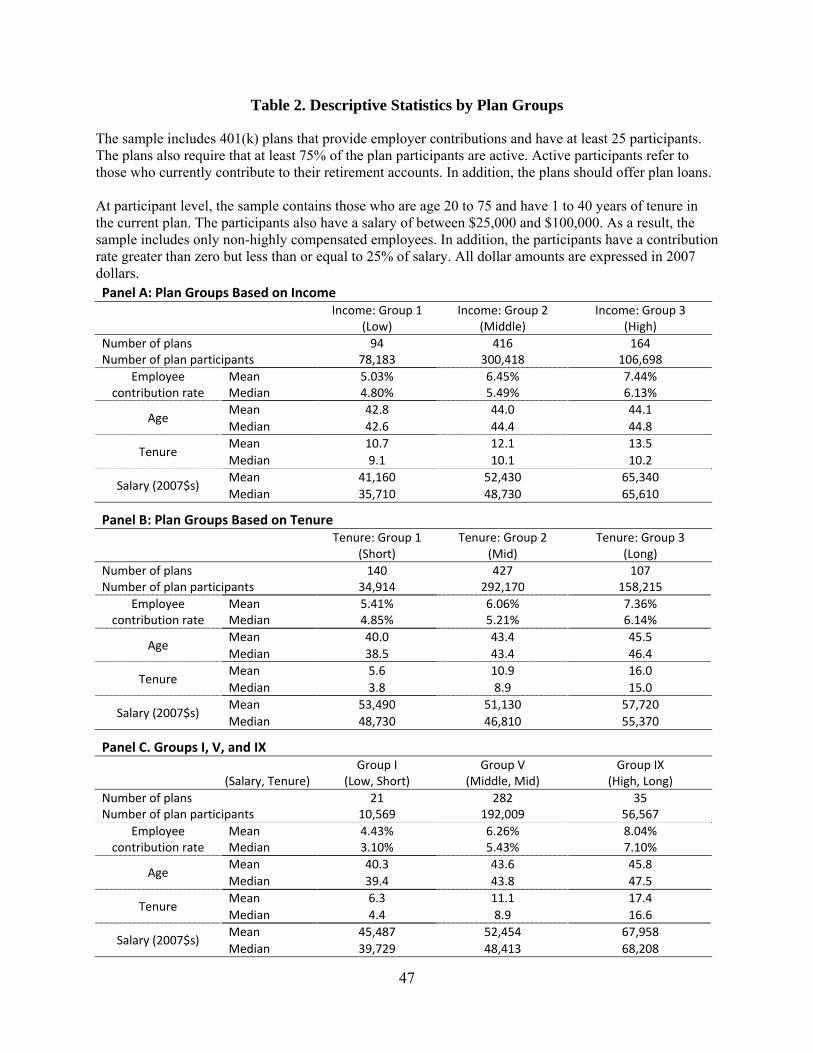
47

Table 2. Descriptive Statistics by Plan Groups

The sample includes 401(k) plans that provide employer contributions and have at least 25 participants. The plans also require that at least 75% of the plan participants are active. Active participants refer to those who currently contribute to their retirement accounts. In addition, the plans should offer plan loans. At participant level, the sample contains those who are age 20 to 75 and have 1 to 40 years of tenure in the current plan. The participants also have a salary of between $25,000 and $100,000. As a result, the sample includes only non-highly compensated employees. In addition, the participants have a contribution rate greater than zero but less than or equal to 25% of salary. All dollar amounts are expressed in 2007 dollars. Panel A: Plan Groups Based on Income Income: Group 1 Income: Group 2 Income: Group 3 (Low) (Middle) (High)

Number of plans 94 416 164 Number of plan participants 78,183 300,418 106,698

Employee Mean 5.03% 6.45% 7.44%contribution rate Median 4.80% 5.49% 6.13%

Age Mean 42.8 44.0 44.1

Median 42.6 44.4 44.8

Tenure Mean 10.7 12.1 13.5

Median 9.1 10.1 10.2

Salary (2007$s) Mean 41,160 52,430 65,340

Median 35,710 48,730 65,610

Panel B: Plan Groups Based on Tenure Tenure: Group 1 Tenure: Group 2 Tenure: Group 3 (Short) (Mid) (Long)



Age Mean 40.0 43.4 45.5

Median 38.5 43.4 46.4

Tenure Mean 5.6 10.9 16.0

Median 3.8 8.9 15.0

Salary (2007$s) Mean 53,490 51,130 57,720

Median 48,730 46,810 55,370

Panel C. Groups I, V, and IX Group I Group V Group IX

(Salary, Tenure) (Low, Short) (Middle, Mid) (High, Long)



Age Mean 40.3 43.6 45.8

Median 39.4 43.8 47.5

Tenure Mean 6.3 11.1 17.4

Median 4.4 8.9 16.6

Salary (2007$s) Mean 45,487 52,454 67,958

Median 39,729 48,413 68,208

48

Table 3. Regression Results This table presents results of ordinary least squares regressions. The dependent variable is the participant contribution rate as a percentage of salary. The participant contribution rate ranges between zero and 25% of salary, the upper bound which is to control for outliers in the distribution of participant contribution rate. The cutoff rate of 25% corresponds to the 98.1th percentile of the distribution of participant contribution rate. As independent variables, the regression includes individual characteristic variables: age, tenure, salary, and loan balance. In particular, tenure refers to the number of years in the current plan. The model also includes plan-level characteristics variables: aggregate employer matching ratio, whether or not to offer company stock, number of funds offered, and plan size expressed as the log number of participants in the plan. In addition, the model includes plan demographics defined by participants’ income and/or tenure. Based on the distribution of salary, a plan with the median income of less than or equal to $35,200 is assigned to a low-income plan group (Income 1), while one with the median income of greater than $63,600 is assigned to a high-income plan group (Income 3). When a plan has the median income of greater than $35,200 and less than or equal to $63,600, it is assigned to a middle-income plan group (Income 2). Similarly, a plan with the median tenure of less than or equal to 5.1 years is assigned to a short-tenure plan group (Tenure 1), while one with the median tenure of greater than 12.4 years is assigned to a long-tenure plan group (Tenure 3). When a plan has the median tenure of longer than 5.1 years and less than or equal to 12.4 years, it is assigned to a mid-tenure plan group (Tenure 2). Plans are further classified into nine groups based on the income and tenure classifications. Panel A presents the regression results with a full sample, while Pane B does the regression results with a subset of the sample: Groups I, V, and IX. All dollar amounts are expressed in 2007 dollars. Standard errors are robust and adjusted for plan-level clustering. ***, ** and * indicate statistical significance 1%, 5% and 10% levels, respectively.

49

Panel A: OLS regressions with a full sample

(1) (2) (3) (4) Variables Coefficient Std. Err. Coefficient Std. Err. Coefficient Std. Err. Coefficient Std. Err.

Constant 5.073 0.656 *** 4.645 0.515 *** 5.895 0.504 *** 5.120 0.405 ***

Age ‐0.143 0.014 *** ‐0.144 0.015 *** ‐0.152 0.014 *** ‐0.148 0.014 ***

Age2 0.0025 0.0002 *** 0.0025 0.0002 *** 0.0026 0.0002 *** 0.0026 0.0002 ***

Tenure 0.079 0.024 *** 0.089 0.021 *** 0.051 0.020 ** 0.068 0.019 ***

Tenure2 ‐0.002 0.001 ** ‐0.002 0.001 *** ‐0.001 0.001 ** ‐0.002 0.001 ***

Salary ($0,000s) 0.453 0.030 *** 0.038 0.027 *** 0.043 0.030 *** 0.377 0.026 ***

Loan balance ($0,000s) ‐0.032 0.108 ‐0.006 0.101 0.000 0.099 ‐0.030 0.098

Aggregate employer matching ratio ‐0.248 0.205 ‐0.180 0.116 ‐0.147 0.092 ‐0.133 0.076 *

Company Stock offered 0.087 0.168 0.022 0.171 0.029 0.165 ‐0.063 0.158

Number of funds 0.016 0.024 0.026 0.022 ‐0.002 0.023 0.016 0.020

(Number of funds)2 ‐0.0002 0.0002 ‐0.0004 0.0002 * 0.0000 0.0002 ‐0.0002 0.0002

ln(Number of participants) ‐0.064 0.067 0.007 0.050 ‐0.090 0.049 * ‐0.007 0.041

Income: Group 2 (reference group)

Income: Group 1 (Income 1) ‐0.957 0.295 ***

Income: Group 3 (Income 3) 0.516 0.178 ***

Tenure: Group 2 (reference group)

Tenure: Group 1 (Tenure 1) ‐0.604 0.234 ***

Tenure: Group 3 (Tenure 2) 0.826 0.219 ***

Income x Tenure: Income 2 and Tenure 2 (Group V: reference group)

Income 1 x Tenure 1 (Group I) ‐1.319 0.346 ***

Income 1 x Tenure 2 (Group II) ‐0.908 0.267 ***

Income 1 x Tenure 3 (Group III) 0.795 0.640

Income 2 x Tenure 1 (Group IV) ‐0.708 0.376 *

Income 2 x Tenure 3 (Group VI) 0.431 0.277

Income 3 x Tenure 1 (Group VII) 0.201 0.286

Income 3 x Tenure 2 (Group VIII) 0.253 0.220

Income 3 x Tenure 3 (Group IX) 0.936 0.243 ***

Number of observations 485,299 485,299 485,299 485,299

Number of plans 674 674 674 674

Adjusted R‐squared 0.10 0.11 0.11 0.12

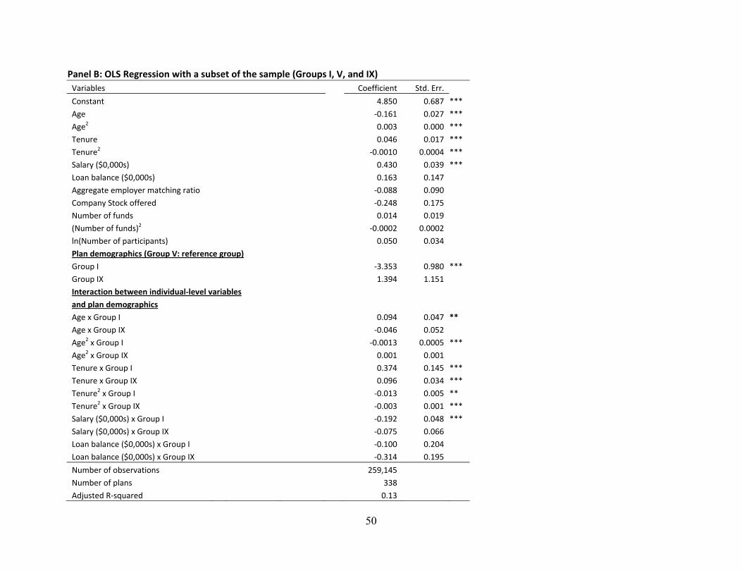
50

Panel B: OLS Regression with a subset of the sample (Groups I, V, and IX)

Variables Coefficient Std. Err.

Constant 4.850 0.687 ***

Age ‐0.161 0.027 ***

Age2 0.003 0.000 ***

Tenure 0.046 0.017 ***

Tenure2 ‐0.0010 0.0004 ***

Salary ($0,000s) 0.430 0.039 ***

Loan balance ($0,000s) 0.163 0.147

Aggregate employer matching ratio ‐0.088 0.090

Company Stock offered ‐0.248 0.175

Number of funds 0.014 0.019

(Number of funds)2 ‐0.0002 0.0002

ln(Number of participants) 0.050 0.034

Plan demographics (Group V: reference group)

Group I ‐3.353 0.980 ***

Group IX 1.394 1.151

Interaction between individual‐level variables

and plan demographics

Age x Group I 0.094 0.047 **

Age x Group IX ‐0.046 0.052

Age2 x Group I ‐0.0013 0.0005 ***

Age2 x Group IX 0.001 0.001

Tenure x Group I 0.374 0.145 ***

Tenure x Group IX 0.096 0.034 ***

Tenure2 x Group I ‐0.013 0.005 **

Tenure2 x Group IX ‐0.003 0.001 ***

Salary ($0,000s) x Group I ‐0.192 0.048 ***

Salary ($0,000s) x Group IX ‐0.075 0.066

Loan balance ($0,000s) x Group I ‐0.100 0.204

Loan balance ($0,000s) x Group IX ‐0.314 0.195

Number of observations 259,145

Number of plans 338

Adjusted R‐squared 0.13

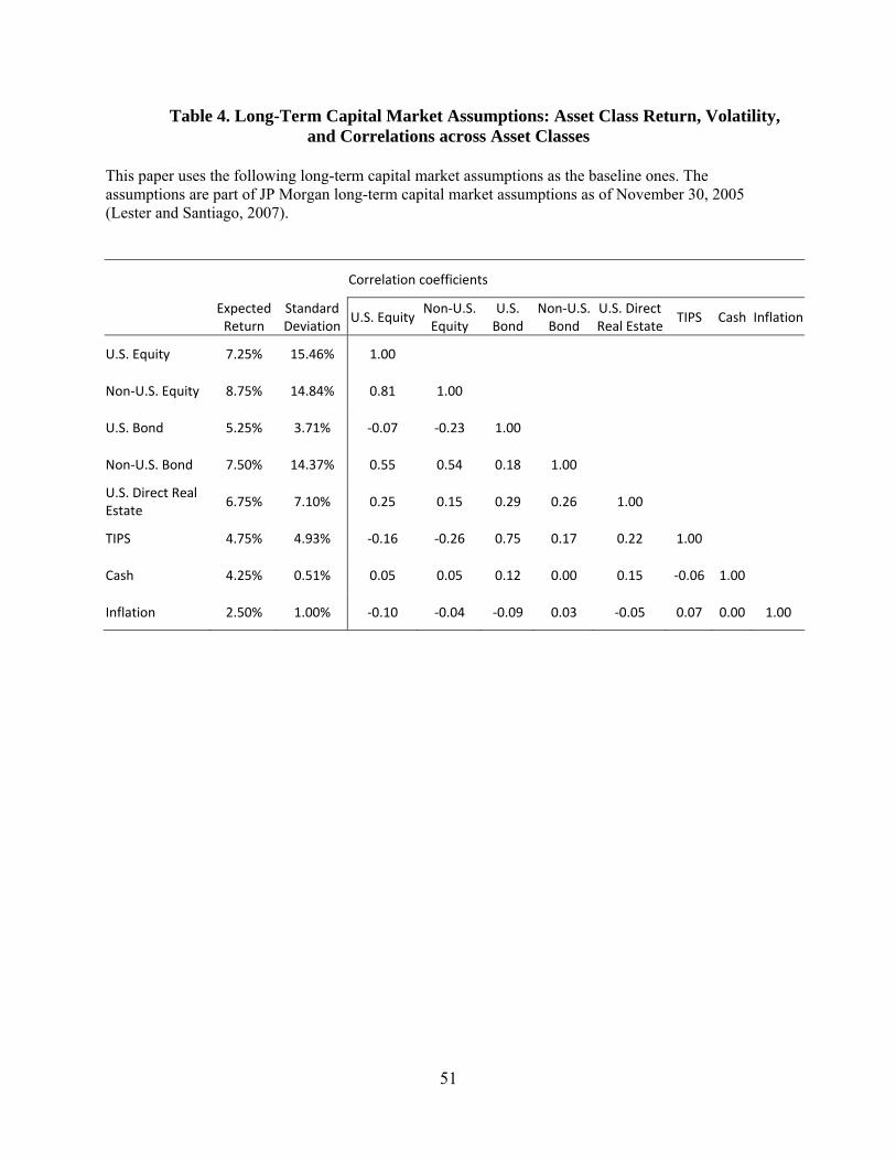
51

Table 4. Long-Term Capital Market Assumptions: Asset Class Return, Volatility, and Correlations across Asset Classes

This paper uses the following long-term capital market assumptions as the baseline ones. The assumptions are part of JP Morgan long-term capital market assumptions as of November 30, 2005 (Lester and Santiago, 2007).

Correlation coefficients

Expected Return

Standard Deviation

U.S. EquityNon‐U.S. Equity

U.S. Bond

Non‐U.S. Bond

U.S. Direct Real Estate

TIPS Cash Inflation

U.S. Equity 7.25% 15.46% 1.00

Non‐U.S. Equity 8.75% 14.84% 0.81 1.00

U.S. Bond 5.25% 3.71% ‐0.07 ‐0.23 1.00

Non‐U.S. Bond 7.50% 14.37% 0.55 0.54 0.18 1.00

U.S. Direct Real Estate

6.75% 7.10% 0.25 0.15 0.29 0.26 1.00

TIPS 4.75% 4.93% ‐0.16 ‐0.26 0.75 0.17 0.22 1.00

Cash 4.25% 0.51% 0.05 0.05 0.12 0.00 0.15 ‐0.06 1.00

Inflation 2.50% 1.00% ‐0.10 ‐0.04 ‐0.09 0.03 ‐0.05 0.07 0.00 1.00

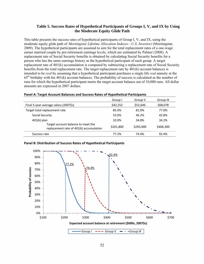
52

Table 5. Success Rates of Hypothetical Participants of Groups I, V, and IX by Using the Moderate Equity Glide Path

This table presents the success rates of hypothetical participants of Group I, V, and IX, using the moderate equity glide path of Morningstar Lifetime Allocation Indexes—U.S. Investors (Morningstar, 2009). The hypothetical participants are assumed to aim for the total replacement rates of a one-wage earner married couple by pre-retirement earnings levels, which are estimated by Palmer (2008). A replacement rate of Social Security benefits is obtained by calculating Social Security benefits for a person who has the same earnings history as the hypothetical participant of each group. A target replacement rate of 401(k) accumulation is computed by subtracting a replacement rate of Social Security benefits from the total replacement rate. The target replacement rate by 401(k) account balances is intended to be real by assuming that a hypothetical participant purchases a single life real annuity at the 65th birthday with his 401(k) account balances. The probability of success is calculated as the number of runs for which the hypothetical participant meets the target account balance out of 10,000 runs. All dollar amounts are expressed in 2007 dollars. Panel A: Target Account Balances and Success Rates of Hypothetical Participants

Group I Group V Group IX

Final 5‐year average salary (2007$s) $42,252 $52,646 $68,078

Target total replacement rate 85.0% 81.0% 77.0%

Social Security 53.0% 46.2% 42.8%

401(k) plan 32.0% 34.8% 34.2% Target account balance to meet thereplacement rate of 401(k) accumulation $201,800 $293,000 $406,300

Success rate 77.2% 74.4% 92.4%

Panel B: Distribution of Success Rates of Hypothetical Participants

0%

10%

20%

30%

40%

50%

60%

70%

80%

90%

100%

$100 $200 $300 $400 $500 $600 $700

Probab

ility of success

Expected account balance at retirement ($000s, 2007$s)


77.2%74.4%

92.4%

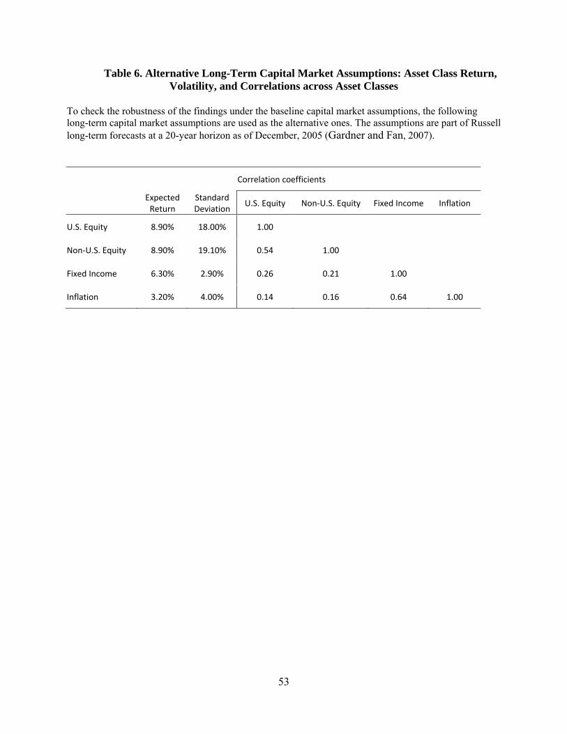
53

Table 6. Alternative Long-Term Capital Market Assumptions: Asset Class Return, Volatility, and Correlations across Asset Classes

To check the robustness of the findings under the baseline capital market assumptions, the following long-term capital market assumptions are used as the alternative ones. The assumptions are part of Russell long-term forecasts at a 20-year horizon as of December, 2005 (Gardner and Fan, 2007).

Correlation coefficients

Expected Return

Standard Deviation

U.S. Equity Non‐U.S. Equity Fixed Income Inflation

U.S. Equity 8.90% 18.00% 1.00

Non‐U.S. Equity 8.90% 19.10% 0.54 1.00

Fixed Income 6.30% 2.90% 0.26 0.21 1.00

Inflation 3.20% 4.00% 0.14 0.16 0.64 1.00

54

Figure 1. Target-Date Fund Equity Glide Paths: Top 20 Largest Target-Date Fund Families and Morningstar® Lifetime Allocation Indexes

Source: Morningstar, 2010. Morningstar® Asset Allocation Indexes, Morningstar, Inc.

55

Figure 2. Estimated Participant Contribution Rate Paths of Groups I, V, and IX This figure is based on the coefficient estimates reported in Panel B of Table 3 and empirical estimates on age, tenure, and salary for each plan group. The figure demonstrates the contribution rates (as a percentage of salary) of the hypothetical participants of Groups I, V, and IX for 40 years (starting at age 25). The hypothetical participants of Group I, V, and IX are assumed to start their working career with a salary of $37,595, $42,759, and $57,899, respectively, each of which is the mean salary at age 25.

0.0

2.0

4.0

6.0

8.0

10.0

12.0

25 30 35 40 45 50 55 60

Participan

t contribution rate (%)

Age


56

Figure 3. Group I: Effects of Target-Date Fund Equity Glide Paths and Automatic Employee Contribution Escalations on Success Rate of the Hypothetical Participant

The figures present the effects of different target-date fund equity glide paths and automatic employee contribution escalations on success rates for Group I (low-income and short-tenure). Panel A demonstrates the change of success rates (Y-axis) by adopting either the conservative or the aggressive equity glide paths instead of the moderate one. X-axis indicates the expected account balances of a 401(k) plan at retirement in 2007 dollars. Panel B demonstrates the variation of success rates at the target account balance of $201,800 by employing different automatic employee contribution escalation arrangements (X-axis). The variation of success rates is expressed as a ratio of the variation of success rates to the maximum success rate (Y-axis, right scale). The panel also includes the probability of success to meet the target account balance by different employee contribution arrangements (Y-axis, left scale).The ratio of the variation of success

rates to the maximum success rate is defined as , ,

, ,, for 0 1. The index k

indicates a path of employee contribution rates until retirement: a hypothetical participant adopts a path of empirically estimated contribution rates of Group I, automatic escalation to 6% (safe harbor minimum), 7%, 8%, 9%, or 10% (safe harbor maximum) of salary. DIFS(sM,sC,sA) represents the difference between the highest success rate and the lowest success rate which can be incurred at a target account balance by three different equity glide paths. Variables sM, sC, and sA indicate the success rates at a target account balance when using moderate, conservative, and aggressive equity glide paths, respectively. MAXS(sM,sC,sA) represents the maximum success rate which can be reached at a target account balance by the three equity glide paths. Thus, the ratio (rk) indicates that, in a given k-path of employee contribution rates, how much variation of success rate a hypothetical participant expects at the maximum success rate by adopting different TDF equity glide paths. The hypothetical participant of Group I is also assumed to aim for a success rate of 85.8%, which is the average of the highest success rates of Groups I, V, and IX when the hypothetical participant follows the empirically estimated contribution rate path of his plan group.

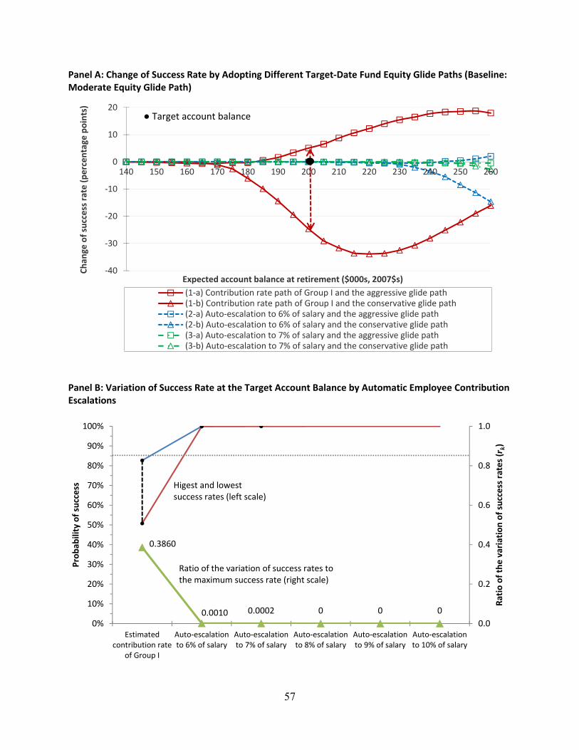
57

Panel A: Change of Success Rate by Adopting Different Target‐Date Fund Equity Glide Paths (Baseline: Moderate Equity Glide Path)

Panel B: Variation of Success Rate at the Target Account Balance by Automatic Employee Contribution Escalations

‐40

‐30

‐20

‐10

0

10

20

140 150 160 170 180 190 200 210 220 230 240 250 260

Chan

ge of success rate (percentage

points)


(1‐a) Contribution rate path of Group I and the aggressive glide path(1‐b) Contribution rate path of Group I and the conservative glide path(2‐a) Auto‐escalation to 6% of salary and the aggressive glide path(2‐b) Auto‐escalation to 6% of salary and the conservative glide path(3‐a) Auto‐escalation to 7% of salary and the aggressive glide path(3‐b) Auto‐escalation to 7% of salary and the conservative glide path

● Target account balance

0.3860

0.0010 0.0002 0 0 0

0.0

0.2

0.4

0.6

0.8

1.0

0%

10%

20%

30%

40%

50%

60%

70%

80%

90%

100%

Estimatedcontribution rate

of Group I

Auto‐escalationto 6% of salary





Ratio of the variation of success rates(r

k)

Probab

ility of success Higest and lowest

success rates (left scale)

Ratio of the variation of success rates to the maximum success rate (right scale)

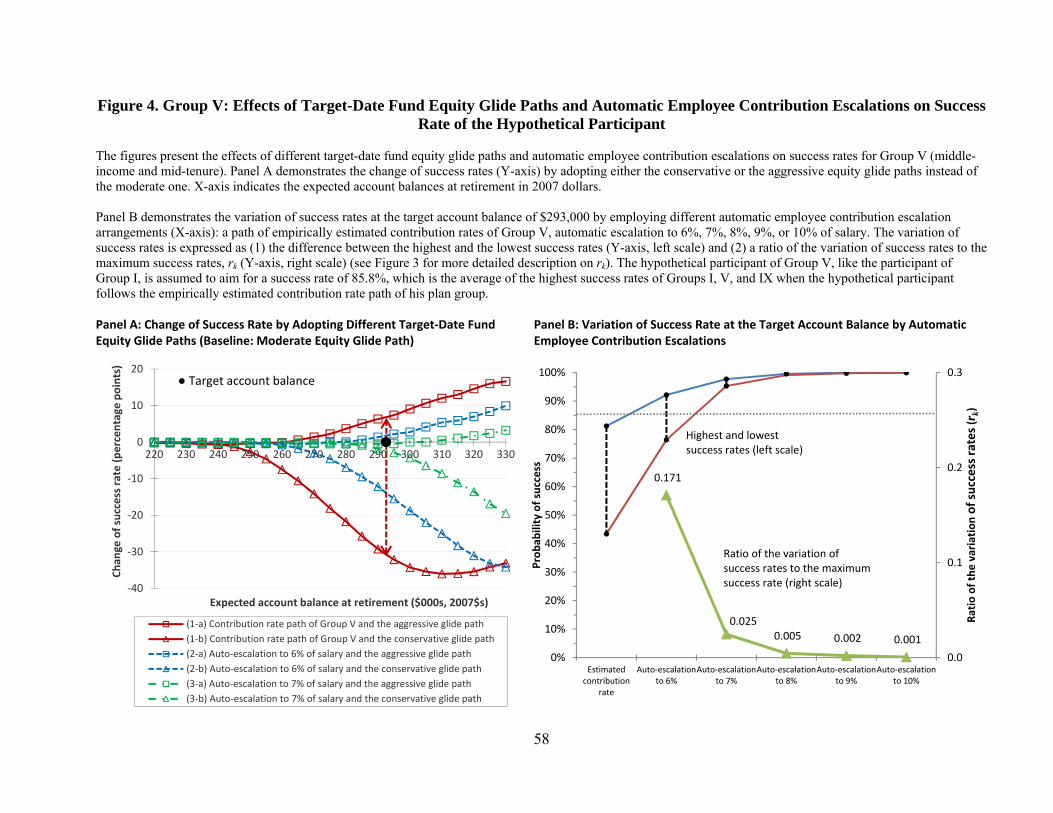
58

Figure 4. Group V: Effects of Target-Date Fund Equity Glide Paths and Automatic Employee Contribution Escalations on Success Rate of the Hypothetical Participant

The figures present the effects of different target-date fund equity glide paths and automatic employee contribution escalations on success rates for Group V (middle-income and mid-tenure). Panel A demonstrates the change of success rates (Y-axis) by adopting either the conservative or the aggressive equity glide paths instead of the moderate one. X-axis indicates the expected account balances at retirement in 2007 dollars. Panel B demonstrates the variation of success rates at the target account balance of $293,000 by employing different automatic employee contribution escalation arrangements (X-axis): a path of empirically estimated contribution rates of Group V, automatic escalation to 6%, 7%, 8%, 9%, or 10% of salary. The variation of success rates is expressed as (1) the difference between the highest and the lowest success rates (Y-axis, left scale) and (2) a ratio of the variation of success rates to the maximum success rates, rk (Y-axis, right scale) (see Figure 3 for more detailed description on rk). The hypothetical participant of Group V, like the participant of Group I, is assumed to aim for a success rate of 85.8%, which is the average of the highest success rates of Groups I, V, and IX when the hypothetical participant follows the empirically estimated contribution rate path of his plan group. Panel A: Change of Success Rate by Adopting Different Target‐Date Fund Equity Glide Paths (Baseline: Moderate Equity Glide Path)


‐40

‐30

‐20

‐10

0

10

20

220 230 240 250 260 270 280 290 300 310 320 330

Chan


points)


(1‐a) Contribution rate path of Group V and the aggressive glide path

(1‐b) Contribution rate path of Group V and the conservative glide path

(2‐a) Auto‐escalation to 6% of salary and the aggressive glide path

(2‐b) Auto‐escalation to 6% of salary and the conservative glide path




0.171

0.025 0.005 0.002 0.001

0.0

0.1

0.2

0.3

0%

10%

20%

30%

40%

50%

60%

70%

80%

90%

100%

Estimatedcontribution

rate

Auto‐escalationto 6%





Ratio of the variationof success rates (r

k)

Probab

ility of success

Highest and lowest success rates (left scale)

Ratio of the variation of success rates to the maximumsuccess rate (right scale)

59

Figure 5. Group IX: Effects of Target-Date Fund Equity Glide Paths and Automatic Employee Contribution Escalations on Success Rate of the Hypothetical Participant

The figures present the effects of different target-date fund equity glide paths and automatic employee contribution escalations on success rates for Group IX (high-income and long-tenure). Panel A demonstrates the change of success rates (Y-axis) by adopting either the conservative or the aggressive equity glide paths instead of the moderate one. X-axis indicates the expected account balances at retirement in 2007 dollars. Panel B demonstrates the variation of success rates at the target account balance of $406,300 by employing different automatic employee contribution escalation arrangements (X-axis): a path of empirically estimated contribution rates of Group IX, automatic escalation to 6%, 7%, 8%, 9%, or 10% of salary. The variation of success rates is expressed as (1) the difference between the highest and the lowest success rates (Y-axis, left scale) and (2) a ratio of the variation of success rates to the maximum success rates, rk (Y-axis, right scale) (see Figure 3 for more detailed description on rk). The hypothetical participant of Group IX, like the participants of Groups I and V, is assumed to aim for a success rate of 85.8%, which is the average of the highest success rates of Groups I, V, and IX when the hypothetical participant follows the empirically estimated contribution rate path of his plan group. Panel A: Change of Success Rate by Adopting Different Target‐Date Fund Equity Glide Paths (Baseline: Moderate Equity Glide Path)


‐40

‐30

‐20

‐10

0

10

20

340 350 360 370 380 390 400 410 420 430 440 450 460

Chan


points)


(1‐a) Contribution rate path of Group IX and the aggressive glide path

(1‐b) Contribution rate path of Group IX and the conservative glide path








0.140

0.022

0.005 0.003

0.0

0.1

0.2

0.3

0%

10%

20%

30%

40%

50%

60%

70%

80%

90%

100%


rate






Ratio of the variationof success rates (r

k)

Probab

ility of success



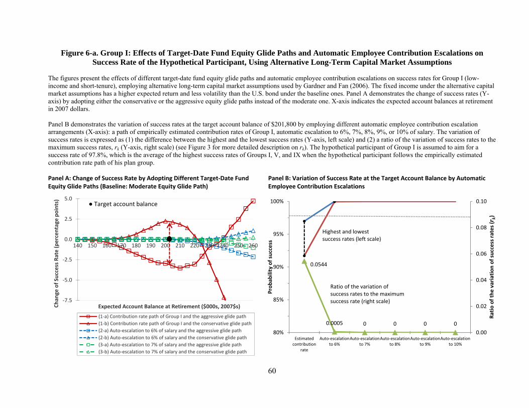
60

Figure 6-a. Group I: Effects of Target-Date Fund Equity Glide Paths and Automatic Employee Contribution Escalations on Success Rate of the Hypothetical Participant, Using Alternative Long-Term Capital Market Assumptions

The figures present the effects of different target-date fund equity glide paths and automatic employee contribution escalations on success rates for Group I (low-income and short-tenure), employing alternative long-term capital market assumptions used by Gardner and Fan (2006). The fixed income under the alternative capital market assumptions has a higher expected return and less volatility than the U.S. bond under the baseline ones. Panel A demonstrates the change of success rates (Y-axis) by adopting either the conservative or the aggressive equity glide paths instead of the moderate one. X-axis indicates the expected account balances at retirement in 2007 dollars. Panel B demonstrates the variation of success rates at the target account balance of $201,800 by employing different automatic employee contribution escalation arrangements (X-axis): a path of empirically estimated contribution rates of Group I, automatic escalation to 6%, 7%, 8%, 9%, or 10% of salary. The variation of success rates is expressed as (1) the difference between the highest and the lowest success rates (Y-axis, left scale) and (2) a ratio of the variation of success rates to the maximum success rates, rk (Y-axis, right scale) (see Figure 3 for more detailed description on rk). The hypothetical participant of Group I is assumed to aim for a success rate of 97.8%, which is the average of the highest success rates of Groups I, V, and IX when the hypothetical participant follows the empirically estimated contribution rate path of his plan group. Panel A: Change of Success Rate by Adopting Different Target‐Date Fund Equity Glide Paths (Baseline: Moderate Equity Glide Path)


‐7.5

‐5.0

‐2.5

0.0

2.5

5.0

140 150 160 170 180 190 200 210 220 230 240 250 260

Chan

ge of Success Rate (percentage

points)

Expected Account Balance at Retirement ($000s, 2007$s)

(1‐a) Contribution rate path of Group I and the aggressive glide path

(1‐b) Contribution rate path of Group I and the conservative glide path






0.0544

0.0005 0 0 0 0

0.00

0.02

0.04

0.06

0.08

0.10

80%

85%

90%

95%

100%


rate






Ratio of the variation of success rates (r

k)

Probab

ility of success



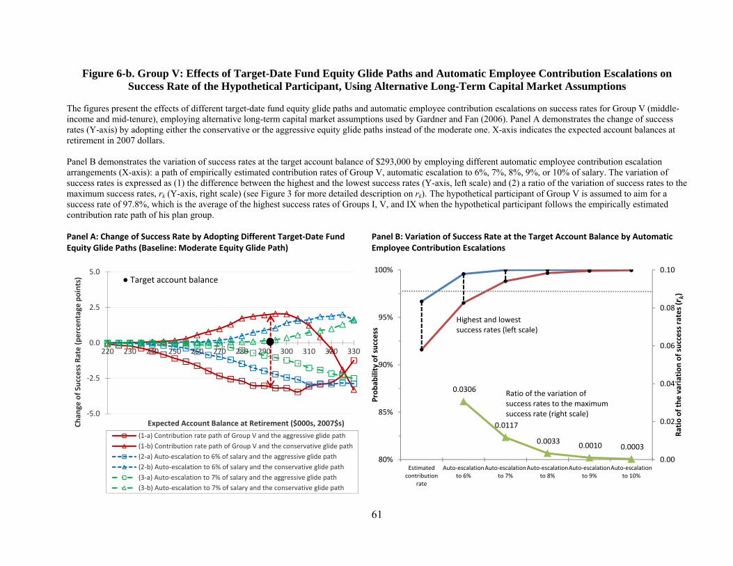
61

Figure 6-b. Group V: Effects of Target-Date Fund Equity Glide Paths and Automatic Employee Contribution Escalations on Success Rate of the Hypothetical Participant, Using Alternative Long-Term Capital Market Assumptions

The figures present the effects of different target-date fund equity glide paths and automatic employee contribution escalations on success rates for Group V (middle-income and mid-tenure), employing alternative long-term capital market assumptions used by Gardner and Fan (2006). Panel A demonstrates the change of success rates (Y-axis) by adopting either the conservative or the aggressive equity glide paths instead of the moderate one. X-axis indicates the expected account balances at retirement in 2007 dollars. Panel B demonstrates the variation of success rates at the target account balance of $293,000 by employing different automatic employee contribution escalation arrangements (X-axis): a path of empirically estimated contribution rates of Group V, automatic escalation to 6%, 7%, 8%, 9%, or 10% of salary. The variation of success rates is expressed as (1) the difference between the highest and the lowest success rates (Y-axis, left scale) and (2) a ratio of the variation of success rates to the maximum success rates, rk (Y-axis, right scale) (see Figure 3 for more detailed description on rk). The hypothetical participant of Group V is assumed to aim for a success rate of 97.8%, which is the average of the highest success rates of Groups I, V, and IX when the hypothetical participant follows the empirically estimated contribution rate path of his plan group. Panel A: Change of Success Rate by Adopting Different Target‐Date Fund Equity Glide Paths (Baseline: Moderate Equity Glide Path)


‐5.0

‐2.5

0.0

2.5

5.0

220 230 240 250 260 270 280 290 300 310 320 330

Chan


points)


(1‐a) Contribution rate path of Group V and the aggressive glide path

(1‐b) Contribution rate path of Group V and the conservative glide path






0.0306

0.0117

0.0033 0.0010 0.0003

0.00

0.02

0.04

0.06

0.08

0.10

80%

85%

90%

95%

100%


rate







k)

Probab

ility of success



62

Figure 6-c. Group IX: Effects of Target-Date Fund Equity Glide Paths and Automatic Employee Contribution Escalations on Success Rate of the Hypothetical Participant, Using Alternative Long-Term Capital Market Assumptions

The figures present the effects of different target-date fund equity glide paths and automatic employee contribution escalations on success rates for Group IX (high-income and long-tenure), employing alternative long-term capital market assumptions used by Gardner and Fan (2006). Panel A demonstrates the change of success rates (Y-axis) by adopting either the conservative or the aggressive equity glide paths instead of the moderate one. X-axis indicates the expected account balances at retirement in 2007 dollars. Panel B demonstrates the variation of success rates at the target account balance of $406,300 by employing different automatic employee contribution escalation arrangements (X-axis): a path of empirically estimated contribution rates of Group IX, automatic escalation to 6%, 7%, 8%, 9%, or 10% of salary. The variation of success rates is expressed as (1) the difference between the highest and the lowest success rates (Y-axis, left scale) and (2) a ratio of the variation of success rates to the maximum success rates, rk (Y-axis, right scale) (see Figure 3 for more detailed description on rk). The hypothetical participant of Group IX is assumed to aim for a success rate of 97.8%, which is the average of the highest success rates of Groups I, V, and IX when the hypothetical participant follows the empirically estimated contribution rate path of his plan group. Panel A: Change of Success Rate by Adopting Different Target‐Date Fund Equity Glide Paths (Baseline: Moderate Equity Glide Path)


‐5.0

‐2.5

0.0

2.5

5.0

340 350 360 370 380 390 400 410 420 430 440 450 460

Chan


points)


(1‐a) Contribution rate path of Group IX and the aggressive glide path(1‐b) Contribution rate path of Group IX and the conservative glide path(2‐a) Auto‐escalation to 6% of salary and the aggressive glide path(2‐b) Auto‐escalation to 6% of salary and the conservative glide path(3‐a) Auto‐escalation to 7% of salary and the aggressive glide path(3‐b) Auto‐escalation to 7% of salary and the conservative glide path(4‐a) Auto‐escalation to 8% of salary and the aggressive glide path(4‐b) Auto‐escalation to 8% of salary and the conservative glide path


0.0353

0.0162

0.00660.0020

0.00

0.02

0.04

0.06

0.08

0.10

80%

85%

90%

95%

100%


rate







k)

Probab

ility of success



401(k) plan participant retirement income security: plan ... meetings/1b-401.pdf ·...

Documents