4. stochastic time series model
TRANSCRIPT

4. Stochastic Time Series Model
• In Chapter 2 and 3 we consider forecast models of the form
zt = f(xt;β) + εt
• In these forecasting models it is usually assumed that the error εt areuncorrelated, which in turn implies that the observations zt are uncorrelated.However this assumption is rarely met in Practice
• Thus models that capture the correlation structure have to be considered.Such as AR(P), MA(q), ARMA(p,q) and ARIMA(d,p,q) will be studied inthis chapter.
1

4.1 Stochastic Processes
• An observed time series (z1, z2, . . . , zn) can be thought of as a particularrealization of a stochastic process.
• Stochastic processes in general can be described by an n-dimensionalprobability distribution p(z1, z2, . . . , zn).
• Assuming joint normality, then there are only n observations but n+(n+1)n/2unknown parameters. To infer such a general probability structure from justone realizations of the stochastic process will be impossible.
• Hence Stationary Assumption is used to simplify the probability structure.
2

3
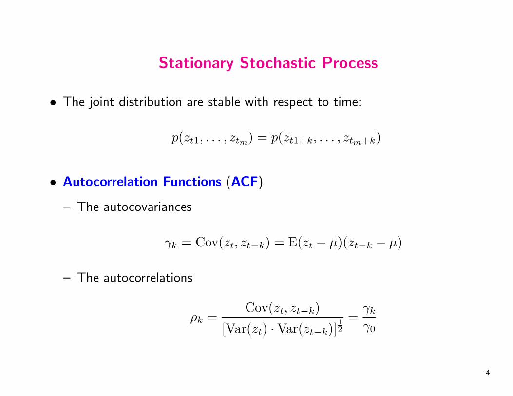
Stationary Stochastic Process
• The joint distribution are stable with respect to time:
p(zt1, . . . , ztm) = p(zt1+k, . . . , ztm+k)
• Autocorrelation Functions (ACF)
– The autocovariances
γk = Cov(zt, zt−k) = E(zt − µ)(zt−k − µ)
– The autocorrelations
ρk =Cov(zt, zt−k)
[Var(zt) ·Var(zt−k)]12
=γk
γ0
4

• Sample Autocorrelation Function (SACF)
rk =
n∑t=k+1
(zt − z)(zt−k − z)
n∑t=1
(zt − z)2, k = 0, 1, 2, . . .
For uncorrelated observations, the variance of rk is approximately given by
Var(rk) ≈1n
5
6

7

4.2 Stochastic Difference Equation Models
• A time series in which successive values are autocorrelated can be representedas a linear combination (linear filter) of a sequence of uncorrelated randomvariables. The linear filter representation is given by
zt − µ = at + ψ1at−1 + ψ2at−2 + · · · =∞∑
j=0
ψjat−j, ψ0 = 1.
The random variable {at; t = 0,±1,±2, . . .} are a sequence of uncorrelatedrandom variable from a fixed distribution with mean E(at) = 0,Var(at) =E(a2
t ) = σ2, and Cov(at, at−k) = E(akat−k) = 0 for all k 6= 0.
• Ezt = µ, γ0 = E(zt − µ)2 = σ2∞∑
j=0
ψ2j ,
γk = E[(zt − µ)(zt−k − µ)] = σ2∞∑
j=1
ψjψj+k,
ρk =
∞∑j=0
ψjψj+k
/∞∑
j=0
ψ2j . 8
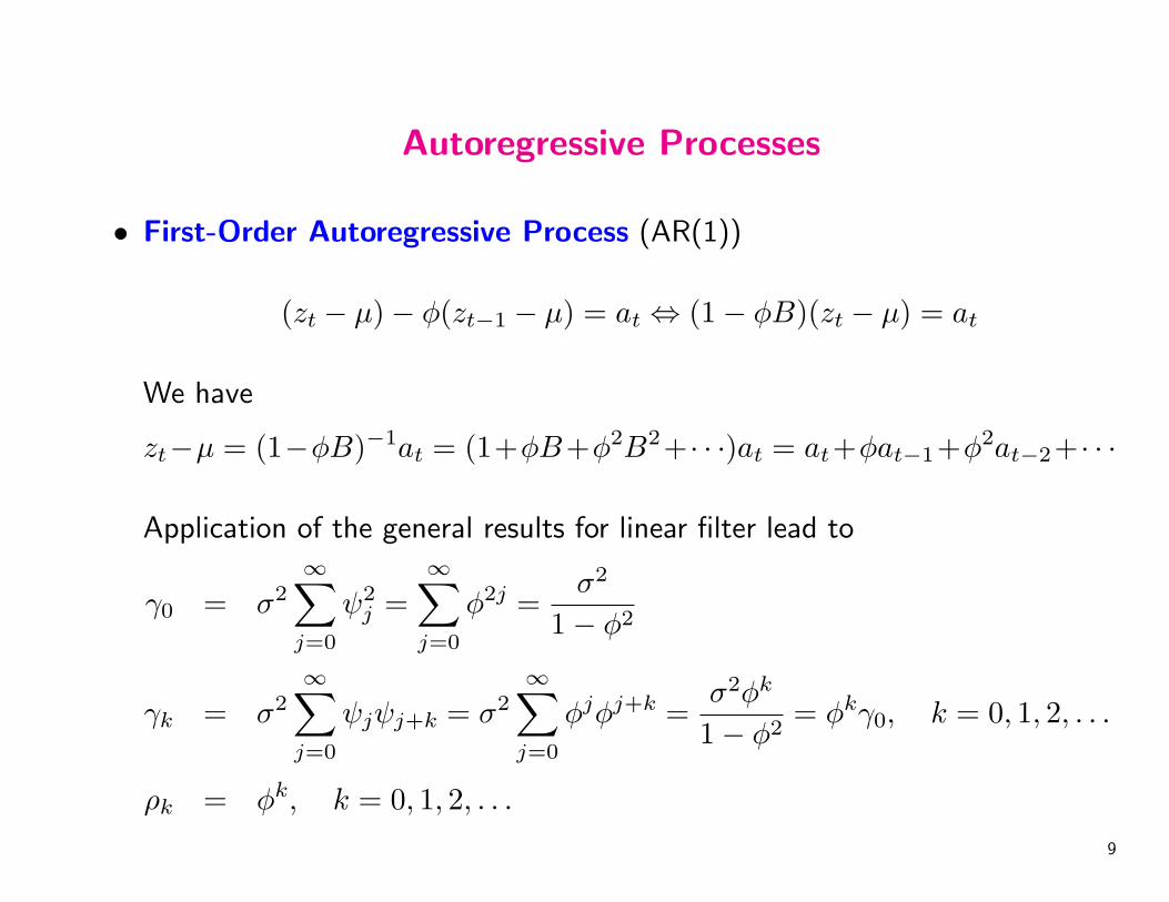
Autoregressive Processes
• First-Order Autoregressive Process (AR(1))
(zt − µ)− φ(zt−1 − µ) = at ⇔ (1− φB)(zt − µ) = at
We have
zt−µ = (1−φB)−1at = (1+φB+φ2B2+ · · ·)at = at+φat−1+φ2at−2+ · · ·
Application of the general results for linear filter lead to
γ0 = σ2∞∑
j=0
ψ2j =
∞∑j=0
φ2j =σ2
1− φ2
γk = σ2∞∑
j=0
ψjψj+k = σ2∞∑
j=0
φjφj+k =σ2φk
1− φ2= φkγ0, k = 0, 1, 2, . . .
ρk = φk, k = 0, 1, 2, . . .9

Another approach to get the ACF for AR(1). This approach is more suitablefor high order situations. Without loss of generality, we assume µ = 0 andzt = φzt−1 + at, then we have
γk = E(ztzt−k) = φE(zt−1zt−k) + E(atzt−k) = φγk−1 + E(atzt−k)
where
k = 0, E(atzt) = E[at(at + φat−1 + φ2at−2 + · · ·)] = σ2
k > 0, E(atzt−k) = 0.
Thus
γ0 = φγ−1 + σ2 = φγ1 + σ2
γk = φγk−1, (k > 1), (γ1 = φγ0)
γ0 = φ2γ0 + σ2 =σ2
1− γ2,
γk = φkγ0,
ρk = φk
10

• Second-Order Autoregression Process [AR(2)]
zt = φ1zt−1 + φ2zt−2 + at
(1− φ1B − φ2B2)zt = at
and
zt =1
1− φ1B − φ2B2at = (1 + ψ1B + ψ2B
2 + · · ·)at
The coefficients (ψ1, ψ2, . . .) could be determined as follows:
1 = (1− φ1B − φ2B2)(1 + ψ1B + ψ2B
2 + · · ·),B : ψ1 − φ1 = 0 ⇒ ψ1 = φ1;
B2 : ψ2 − φ1ψ2 − φ2ψ1 = 0 ⇒ ψ2 = φ21 + ψ2;
B3 : ψ3 − φ1ψ2 − φ2ψ1 = 0 ⇒ ψ3 = φ31 + 2φ1φ2;
ψj = φ1ψj−1 + φ2ψj−2, j ≥ 2.
11

12

• Stationarity
AR(p) : (1− φ1B − φ2B2 − · · · − φpB
p) = (1−G1B) · · · (1−GpB).
The stationarity relates to the conditions: |G−1i | > 1, i = 1, 2, . . . , p..
Particulary for AR(2), the stationarity corresponds to
φ1 + φ2 < 1, φ2 − φ1 < 1,−1 < φ2 < 1.
• ACF of AR(2)
E(ztzt−k) = φE(zt−1zt−k) + φE(zt−2zt−k) + E(zt−kat).
γ0 = φ1γ1 + φ2γ2 + σ2,
γk = φ1γk−1 + φ2γk−2, k ≥ 1.
ρk = φ1ρk−1 + φ2ρk−2.
(1− ρ1B − ρ2B2)ρk = 0. k = 1, 2, . . .
•
13

Actually the general solution of the difference equation:
(1− φ1B − φ2B2)ρk = 0
is
ρk =
A1G
k1 +A2G
k2 (G1 6= G2),
(A1 +A2k)Gk, (G1 = G2 = G),{A1 sin(θk) +A2 cos(θk)}(p2 + q2)−k/2, p± qi = G−1
1,2,
θ = arcsin(p2/√p2 + q2)
So, when stationary, the correlogram shows damped exponentials/sinusoidalwaves.
14

15

• The general AR(p) model
γ0 = φ1γ1 + · · ·+ φpγp + σ2 =σ2
1− φ1ρ1 − · · · − φpρp=
σ2
φ(B)ρ0
γk = φ1γk−1 + · · ·+ φpγk−p, k > 0
ρk = φ1ρk−1 + · · ·+ φpρk−p.
– Letting k = 1, 2, . . . , p, we have the Yule-walker equations:
ρ = Pφ,
P =
1 ρ1 ρ2 · · · ρp−1
ρ1 1 ρ1 · · · ρp−2... . . . . . . ... ...
ρp−1 ρp−2 ρp−3 · · · 1
– Moments Methods:
φ = P−1ρ
16

Partial Autocorrelations
When considering two random variables’ correlation coefficient, it would be fairif we could get ride of the influence of other random variables related to them.In the AR(p) model: assuming the stability
zt = φk1zk−1 + φk2zt−2 + · · ·+ φkkzt−k + at ⇒ φzt = at
implies φ(B) has all the roots outside the unit circle. Therefore |φkk| < 1.
This is defined as the partial autocorrelation between zt and zt−k.
• AR(1): zt = φ11zt−1 + at ⇒ φ11 = ρ1.
• AR(2): ρ1 = φ21 + ρ1φ22, ρ2 = ρ1φ21 + φ22 ⇒ φ22 = ρ2−ρ21
1−ρ21
17

• AR(p): Using Yule-walker Equationsρ1
ρ2...ρk
=
1 ρ1 · · · ρk−1
ρ1 1 · · · ρk−2... ... . . . ...
ρk−1 ρk−2 · · · 1
φk1
φk2...φkk
φkk =
∣∣∣∣∣∣∣∣1 ρ1 · · · ρk−2 ρ1
ρ1 1 · · · ρk−3 ρ2... ... . . . ... ...
ρk−1 ρk−2 · · · ρ1 ρk
∣∣∣∣∣∣∣∣∣∣∣∣∣∣∣∣
1 ρ1 · · · ρk−1
ρ1 1 · · · ρk−2... ... . . . ...
ρk−1 ρk−2 · · · 1
∣∣∣∣∣∣∣∣−1
• The basic features of AR(p):
– ACF: Combinations of damped exponentials/sinusodal waves;– PACF: zero for lags larger than p.
18

• Sample Partial Autocorrelation Functions (SPAF)
1. Use the sample correlation coefficient rj in place of ρj and solve theYule-Walker equation for ρkk. This scheme is impractical if lag k is large.
2. Recursive forms:
φkk =rk −
k−1∑j=1
φk−1,jrk−j
1−k−1∑j=1
φk−1,jrj
,
φk,j = φk−1,j − φkkφk−1,k−j, j = 1, 2, . . . , k − 1.
3. Standard Errors of φkk
If the data follow an AR(p) process, then for lags greater than p thevariance of φkk can be approximated by
Var(φ) ≈ n−1 for k > p.
Approximate standard error for φkk are given by n−1/2.19

20
21

Moving Average MA(q) Model
zt − µ = (1− θ1B − θ2B2 − · · · − θqB
q)at = θ(B)at
• Autocovariances and Autocorrelations
γ0 = (1 + θ21 + · · ·+ θ2q)σ2
γk = (−θk + θ1θk+1 + · · ·+ θq−kθq)σ2, k = 1, 2, . . . , q
γk = 0, k > q
ρk =−θk + θ1θk+1 + · · ·+ θq−kθq
1 + θ21 + · · ·+ θ2q, k = 1, 2, . . . , q
ρk = 0, k > q
• Partial Autocorrelation Function for MA Process
The ACF of a moving average process of order q cuts off after lag q(ρk = 0, k > q). However, its PACF is infinite in extent (it tails off).
In General, the PACF is dominated by combinations of damped exponentialsand/or damped sine waves.
22

• Example: MA(1) Model: zt − µ = at − θat−1
γ0 = (1 + θ2)σ2
γ1 = −θσ2
ρ1 =−θ
1 + θ2; (|θ| < 1
2), ρk = 0, k > 1
Invertibility condition: since both (θ, 1/θ) are roots of the equation
θ2ρ1 + θ + ρ1 = 0,
so we restrict ourselves to the situation with |θ| < 1 so that the model couldinvert to the AR from
zt − µ = π1(zt−1 − µ) + π2(zt−2 − µ) + · · ·+ at
where∑∞
j=1 |πj| < +∞.For MA(1) Model
πj = −θj, (|θ| < 1), φkk =−θk(1− θ2)1− θ2(k+1)
, k > 0.23

24

Autoregressive Moving Average (ARMA(p,q)) Processes
(1− φ1B − · · ·φpBp)(zt − µ) = (1− θ1B − · · · − θqB
q)at
or
zt − µ = φ1(zt−1 − µ) + · · ·+ φp(zt−p − µ)
+ at − θ1at−1 − · · · − θqat−q
• k > q − p, ACF dominated by AR part
• k > p− q, PACF dominated by MA part
SummaryThe ACF and PACF of a mixed ARMA(p,q) process are both infinite in extentand tail off (die down) as the lag k increases. Eventually (for k > q − p), theACF is determined from the autoregressive part of the model. The PACF iseventually (for k > p− q) determined from moving average part of model.
25

• ARMA(1,1) Process
(1− φB)(zt − µ) = (1− θB)at
– ACF:
γ0 =1 + θ2 − 2φθ
1− φ2σ2,
γ1 =(1− φθ)(φ− θ)
1− φ2σ2,
ρ1 =(1− φθ)(φ− θ)1 + θ2 − 2φθ
ρk = φρk−1, k > 1.
– PACF: φ11 = ρ1, then similar to MA(1)
26
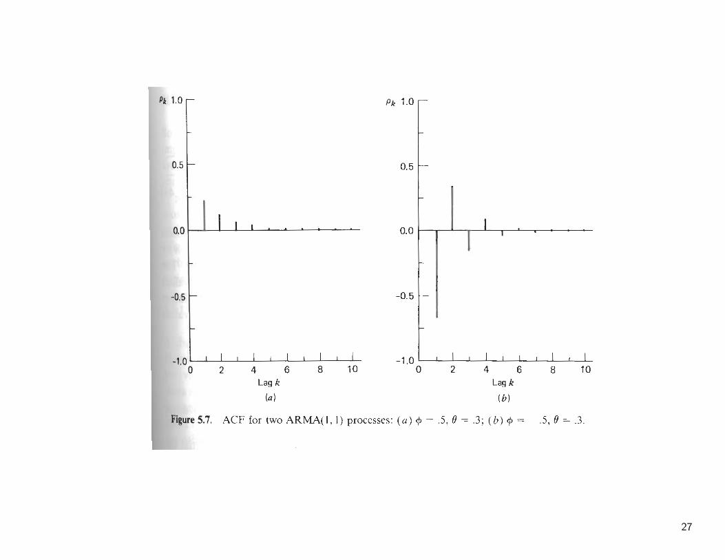
27

4.3 Nonstationary processes
• Nonstationary, Differencing, and Transformations
M1: zt = β0 + β1t+ at
M2: (1−B)zt = β1 + at or zt = Zt−1 + β1 + at.M3: (1−B)2zt = at or zt = 2zt−1 − zt−2 + at.
• Nonstationary Variance
• Examples: 1. Growth rates. 2. Demand for repair parts.
28

29

30

31

32

An Alternative Argument for Differencing
Let us assume that data zt are described by a nonstationary level
µt = E(zt) = β0 + β1t
and that we wish to entertain an ARMA model for a function of zt that has alevel independent of time.
• Consider the model φp+1(B)zt = θ0 + θ(B)at
• θ0 represent the level of φp+1(B). To achieve a θ0 that is constant,independent of time,
φp+1(B) = (1−B)φ(B)
and
θ0 = φp+1(B)(β0 + β1t) = φ(B)(1−B)(β0 + β1) = φ(B)β1
33

• If µt = β0 + β1t+ · · ·+ βdtd, we have to choose the autoregressive operator
in φp+d(B)zt = θ0 + θ(B)at such that
φp+d(B) = (1−B)dφ(B)
and then
θ0 = φp+d(B)(β0 + β1t+ · · ·+ βdtd)
= φ(B)(1−B)d(β0 + β1t+ · · ·+ βdtd)
= φ(B)βdd!.
34

Autoregressive Integrated Moving Average (ARIMA) Models
• Transform a nonstationary series zt into a stationary one by consideringrelevant differences
wt = ∇dzt = (1−B)dzt.
• Then use the ARMA models to describe wt. The corresponding model canbe written as
φ(B)wt = θ0 + θ(B)at
orφ(B)(1−B)dzt = θ0 + θ(B)at
• ARIMA(p,d,q) The order p, d, q are usually small. The model is called“integrated”, since zt can be thought of as the summation (integration) ofthe stationary series wt. For example, if d = 1
zt = (1−B)−1wt =t∑
k=−∞
wk
35

Choice of the proper degree of differencing
• Plot of the series
• Examination of the SACFA stationary AR(p) process requires that all Gi in
(1− φ1B − · · · − φpBp) = (1−G1B) · · · (1−GpB)
are such that |Gi| < 1 (i = 1, 2, . . . , p), Now assume one of them, say G1,approaches 1, that is G1 = 1− δ, where δ is a small positive number. Thenthe autocorrelations
ρk = A1Gk1 + · · ·+ApG
kp∼= A1G
k1.
So the exponential decay will be show and almost linear [i.e. A1Gk1 =
A1(1− δ)k ∼= A1(1− δk)]
36

• Consider the ARMA(1,1) model
(1− φB)zt = (1− θB)at
The ACF of this process is given by
ρ1 =(1− φθ)(φ− θ)1 + θ2 − 2φθ
ρk = φkρ1
• If we let φ→ 1, then ρk → 1 for any finite k > 0. Again the autocorrelationdecay very slowly when φ is near 1.
• It should be pointed out that the slow decay in the SACF can start at valuesof r1 considerably smaller that 1.
37
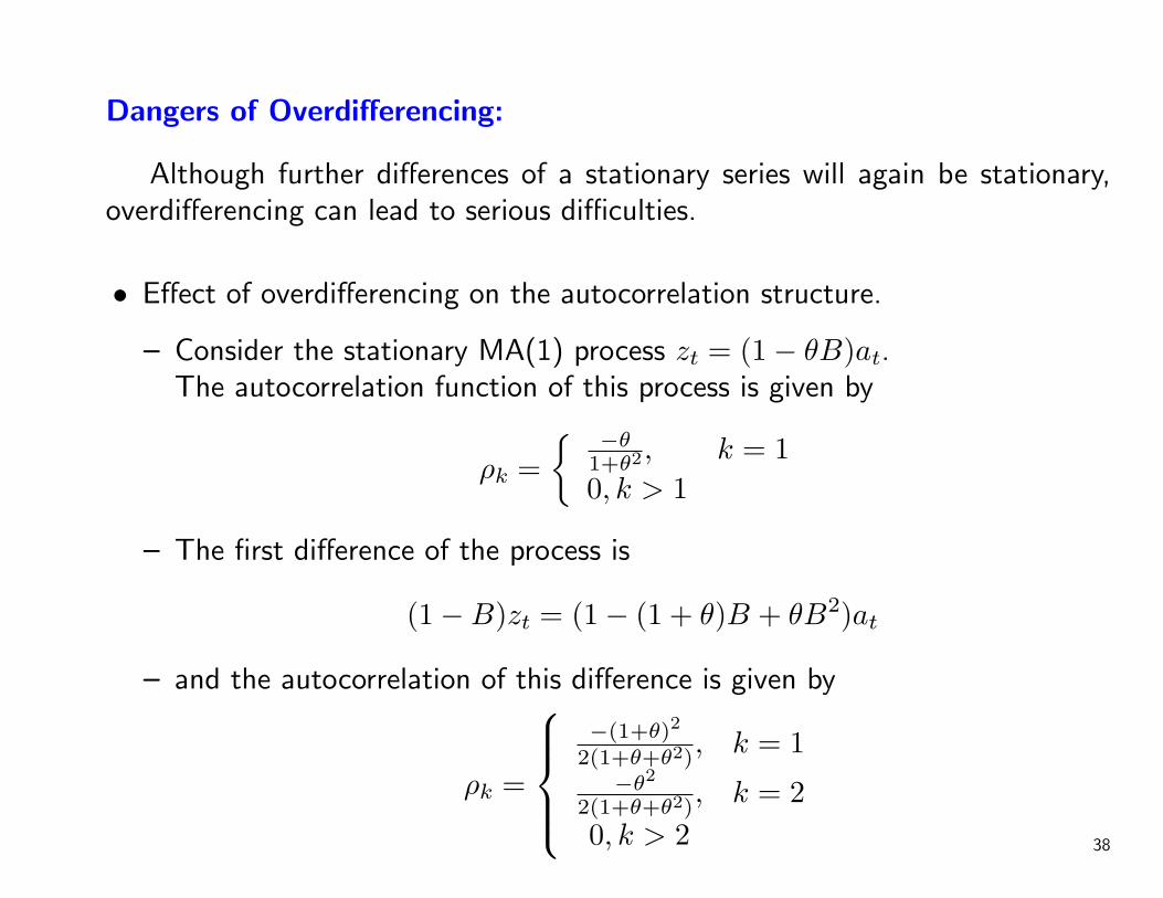
Dangers of Overdifferencing:
Although further differences of a stationary series will again be stationary,overdifferencing can lead to serious difficulties.
• Effect of overdifferencing on the autocorrelation structure.
– Consider the stationary MA(1) process zt = (1− θB)at.The autocorrelation function of this process is given by
ρk ={ −θ
1+θ2, k = 10, k > 1
– The first difference of the process is
(1−B)zt = (1− (1 + θ)B + θB2)at
– and the autocorrelation of this difference is given by
ρk =
−(1+θ)2
2(1+θ+θ2), k = 1
−θ2
2(1+θ+θ2), k = 2
0, k > 2 38

• Effect of overdifferencing on variance.
– Consider the same MA(1) process. Its variance is given by
γ0(z) = (1 + θ)2σ2
– The variance of the overdifferenced series wt = (1 − B)zt, which followsan MA(2) process, is given by
γ0(w) = 2(1 + θ + θ2)σ2
– Henceγ0(w)− γ0(z) = (1 + θ2)σ2 > 0
39

• Considered the stationary process AR(1) process (1 − φB)zt = at withvariance
γ0 =σ2
1− φ2
• The first difference wt follows the ARMA(1,1) process (1 − φB)wt = (1 −B)at. The variance of this process is given by
γ0(w) =2(1− φ)σ2
1− φ2
• and
γ0(w)− γ0(z) =(1− 2φ)σ2
1− φ2
Hence when φ < 12, overdifferencing will increasing the variance.
40

Regression and ARIMA Models
• ARIMA(0,1,1) model (1−B)zt = (1− θB)at
– Since ψ(B) = (1− θB)/(1−B) = 1+(1− θ)B+(1− θ)B2 + · · ·, we canrelated the variable zt+l at time t+ l to a fixed origin t and express it as
zt+l = β(t)0 + et(l)
– where et(l) = at+l+(1−θ)[at+l−1+· · ·+at+1] is a function of the random
shocks that enter the system after time t, and β(t)0 = (1 − θ)
∑tj=−∞ aj
depends on all the shock (observations) up to and including time t.
– The level β(t)0 can be updated according to
β(t+1)0 = β
(t)0 + (1− θ)at+1
– In the special case when θ = 1, et(l) = at+l and β(l+1)0 = β
(t)0 = β0. In this
case, the model is equivalent to the constant mean model zt+l = β0+at+l.
41

• ARIMA(0,2,2) model (1−B)2zt+l = (1− θ1B − θ2B2)at+l
– Using an argument similar to that followed for ARIMA(0,1,1) model, theARIMA(0,2,2) can be written as
zt+l = β(t)0 + β
(t)1 l + et(l)
where et(l) are correlated and given by
et(l) = at+l + ψ1at+l−1 + · · ·+ ψl−1at+1
– where the ψ weights may be obtained from
(1 + ψ1B + ψ2B2 + · · ·)(1−B)2 = 1− θ1B − θ2B
2
These ψ weights can be given as ψj = (1 + θ2) + j(1− θ1 − θ2), j ≥ 1.
42
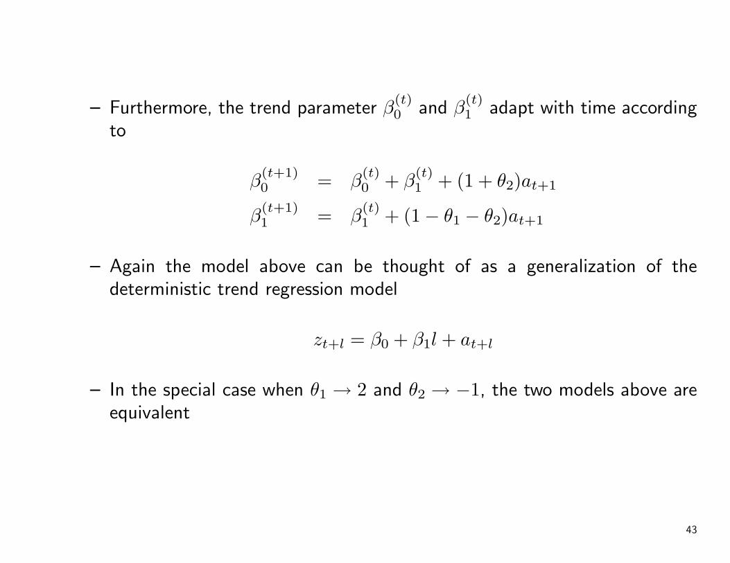
– Furthermore, the trend parameter β(t)0 and β
(t)1 adapt with time according
to
β(t+1)0 = β
(t)0 + β
(t)1 + (1 + θ2)at+1
β(t+1)1 = β
(t)1 + (1− θ1 − θ2)at+1
– Again the model above can be thought of as a generalization of thedeterministic trend regression model
zt+l = β0 + β1l + at+l
– In the special case when θ1 → 2 and θ2 → −1, the two models above areequivalent
43

44
45

4.4 Forecasting
• ARIMA model φ(B)(1−B)dzt = θ(B)at
• Autoregressive representation
zt = π1zt−1 + π2zt−2 + · · ·+ at
where the π weights are given by
1− πB − πB2 − · · · = φ(B)(1−B)d
θ(B)
• l-step forecastzl = η0zn + η1zn−1 + η2zn−2 + · · ·
orzl = ξ0an + ξ1an−1 + ξ2an−2 + · · ·
46
Minimum mean square error (MMSE) forecasts: The mean square errorE[zn+l − zn(l)]2 is minimized.
• Using the ψ weights in ψ(B) = θ(B)φ−1(B)(1 − B)−d to write the modelin its linear filter representation
zn+l = an+l + ψ1an+l−1 + · · ·+ ψl−1an+1 + ψlan + ψl+1an−1 + · · ·
• Then the mean square error is expressed as
E[zn+l − zn(l)] = E[an+l + an+l−1 + · · ·+ ψl−1an+1 + (ψl − ξ0)an
+(ψl+1 − ξ1)an−1 + · · ·]2
= (1 + ψ21 + · · ·+ ψ2
l−1)σ2 +
∞∑j=0
(ψl+j − ξj)2σ2.
47
• The minimum mean square error (MMSE) forecast
zn(l) = ψlan + ψl+1an−1 + · · ·
• The forecast error is given by
en(l) = zn+l − zn(l) = an+l + ψ1an+l−1 + · · ·+ ψl−1an+1
and its variance by
Var[en(l)] = σ2(1 + ψ21 + ψ2
2 + · · ·+ ψ2l−1)
•E(an+j|zn, zn−1, . . .) =
{an+j j ≤ 00 j > 0
Hence
E(zn+l|zn, zn−1, . . .) = E[(an+l + ψ1an+l−1 + · · ·+ ψl−1an+1
+ψlan + ψl+1an−1 + · · ·)|zn, zn−1, . . .]
= ψlan + ψl+1an−1 + · · · 48
Examples:
• AR(1) process: zt − µ = φ(zt−1 − µ) + at
• AR(2) process: zt = φ1zt−1 + φ2zt−2 + at
• ARIMA(0,1,1) process: zt = zt−1 + at − θat−1
• ARIMA(1,1,1) process: (1− φB)(1−B)zt = θ0 + (1− θB)at or
zt = θ0 + (1 + φ)zt−1 − φzt−2 + at − θat−1
• ARIMA(0,2,2) process: (1−B)2zt = (1− θ1B − θ2B2)at or
zt = 2zt−1 − zt−2 + at − θ1at−1 − θ2at−2
49

Prediction Limits
• It is usually not sufficient to calculate point forecast alone. The uncertaintyassociated with a forecast should be expressed, and the prediction limitsshould always be computed.
• It is possible, but not very easy, to calculate a simultaneous “predictionregion” for a set of future observations. Therefore, we give probability limitsonly for individual forecasts.
• Assuming that at’s (and hence the z’s) are normally distributed, we cancalculate 100(1− λ) percent prediction limits form
zn(l)± uλ/2{V (en(l))}1/2
where uλ/2 is the 100(1 − λ/2) percentage point of standard normaldistribution.
50

• Because zn(l) and V (en(l)) are unknown exactly, and need estimate. Hencethe estimated prediction limits are given by
zn(l)± uλ/2{V (en(l))}1/2
• Consider AR(1) process for Yield data, we found z156(1) = 0.56, z156(2) =0.62, z156(3) = 0.68, V [e156(1)] = 0.024, V [e156(2)] = 0.041, V [e156(1)] =0.054. Thus the 95 percent prediction limits for z156+l, l = 1, 2, 3 are givenby
z157 : z156(1)± 1.96{V [e156(1)]}1/2 = .56± 1.96(.15) = .56± .29
z158 : z156(2)± 1.96{V [e156(2)]}1/2 = .62± 1.96(.20) = .62± .39
z159 : z156(3)± 1.96{V [e156(3)]}1/2 = .68± 1.96(.23) = .68± .45
51

Forecast Updating
• Suppose we are at time n and we are predicting l + 1 steps ahead. Theforecast is given by
zn(l + 1) = ψl+1an + ψl+2an−1 + · · ·
• After zn+1 has become available, we need to update our prediction of zn+l+1.On the other hand zn+1(l) can be written as
zn+l = ψlan+1 + ψl+1an + ψl+2an−1 + · · ·
• we find that
zn+1(l) = zn(l + 1) + ψlan+1 = zn(l + 1) + ψl(zn+1 − zn(l))
• The updated forecast is a linear combination of the previous forecast ofzn+l+1 made at time n and the most recent one-step-ahead forecast erroren(l) = zn+1 − zn(l) = an+1.
52

Use Yield data example as shown as before. We already obtained the forecastfor z157, z158, z159 from time origin n = 156. Suppose now that z157 = 0.74 isobserved and we need to update the forecasts for z158 and z159.
• Since the model under consideration is AR(1) with the parameter estimateφ = 0.85, the estimated ψ weights are given by ψj = φj = 0.85j.
• Then the updated forecasts are given by
z158 : z156(2) + ψ1[z157 − z156(1)] = 0.62 + 0.85(0.74− 0.56) = 0.77
z159 : z156(3) + ψ2[z157 − z156(1)] = 0.62 + 0.852(0.74− 0.56) = 0.81
• The updated 95 percent prediction limits for z158 and z159 become
z158 : z157(1)± 1.96{V [e157(1)]}1/2 = .77± .29
z159 : z157(2)± 1.96{V [e157(2)]}1/2 = .81± .3953

4.5 Model Specification
Step 1. Variance-stabilizing transformations. If the variance of the series changeswith the level, then a logarithmic transformation will often stabilize thevariance. If the logarithmic transformation still not stabilize the variance, amore general approach and employ the class of power transformations canbe adopted.
Step 2. Degree of differencing. If the series or its appropriate transformation is notmean stationary, then the proper degree of differencing has to determined.For the series and its differences, we can examine
1. Plots of the time series2. Plot of the SACF3. Sample variances of the successive differences
54
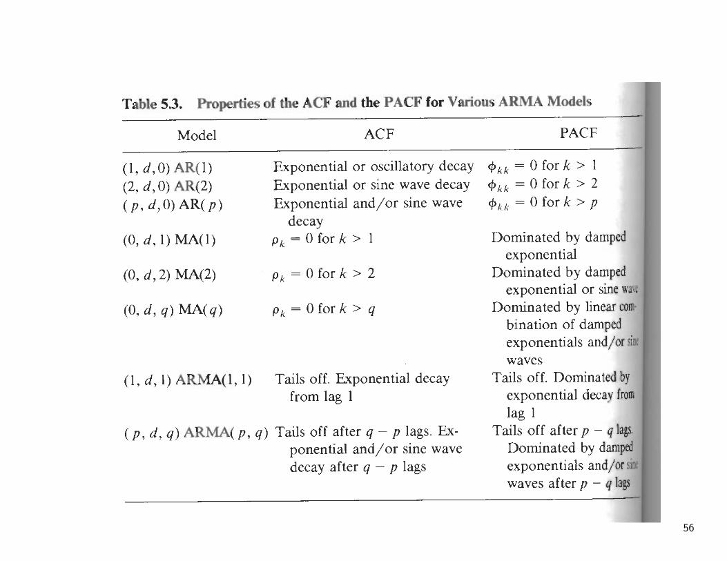
Step 3. Specification of p and q. Once we obtain a stationary difference wemust specify the orders of the autoregressive (p) and moving average (q)polynomials. The orders can be specified by matching the patterns inthe sample autocorrelations and partial autocorrelations with the theoreticalpatterns of known models (See Table 5.3).
Step 4. Inclusion of a trend parameter. If the series requires differencing, weshould check whether it is necessary to include a deterministic trend θ0 inthe model. This can be done by comparing the sample mean w of thestationary difference with its standard error s(w). This standard error can beapproximated by
s(w) ∼=[c0n
(1 + 2r1 + 2r2 + · · ·+ 2rk)]1/2
where c0 is the sample variance and r1, · · · , rk are the first K significantsample autocorrelations of the stationary differences. This approximation isappropriate only if s(w) > 0.
55
56

4.6∗ Model Estiamtion
After specifying the form of the model, it is necessary to estimate its parameters.Let (z1, z2, . . . , zN) represent the vector of the original observations and w =(w1, . . . , wn)′ the vector of the n = N − d stationary differences.
Maximum Likelihood Estimates
• The ARIMA model can be written as
at = θ1at−1 + · · ·+ θqat−q + wt − φ1wt−1 − · · · − φpwt−p
• The joint probability density function of a = (a1, a2, . . . , an)′ is given by
p(a|φ, θ, σ2) = (2πσ2)−n/2 exp
[− 1
2σ2
n∑t=1
a2t
]
57

• The joint probability density function of w can be written down, at least inprinciple. It is of the form
L(φ, θ, σ2|w) = g1(φ, θ, σ2) exp[− 1
2σ2S(φ, θ)
]
where g1 is a function of the parameter (φ, θ, σ2) and
S(φ, θ) =n∑
t=1−p−q
E2(ut|w)
E(ut|w) = E(ut|w, φ, θ, σ2) is the conditional expectation of ut given w, φ, θand σ2, and
ut ={at, t = 1, 2, . . . , ng2(a∗,w∗), t ≤ 0
where g2 is a linear function of the initial unobservable values a∗ =(a1−q, . . . , a−1, a0)′ and w∗ = (w1−p, . . . , w−1, w0)′.
58
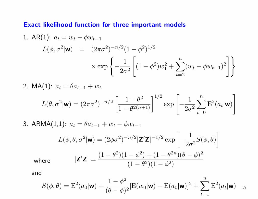
Exact likelihood function for three important models
1. AR(1): at = wt − φwt−1
L(φ, σ2|w) = (2πσ2)−n/2(1− φ2)1/2
× exp
{− 1
2σ2
[(1− φ2)w2
1 +n∑
t=2
(wt − φwt−1)2]}
2. MA(1): at = θat−1 + wt
L(θ, σ2|w) = (2πσ2)−n/2
[1− θ2
1− θ2(n+1)
]1/2
exp
[− 1
2σ2
n∑t=0
E2(at|w)
]
3. ARMA(1,1): at = θat−1 + wt − φwt−1
L(φ, θ, σ2|w) = (2φσ2)−n/2|Z′Z|−1/2 exp[− 1
2σ2S(φ, θ)
]where |Z′Z| = (1− θ2)(1− φ2) + (1− θ2n)(θ − φ)2
(1− θ2)(1− φ2)and
S(φ, θ) = E2(a0|w) +1− φ2
(θ − φ)2[E(w0|w)− E(a0|w)]2 +
n∑t=1
E2(at|w) 59

Maximum likelihood Estimate (MLE) of parameters (φ, θ, σ2) for theARIMA model can be obtained by maximizing the likelihood function. Ingeneral, closed-form solutions cannot be found. However, various algorithmsare available to compute the MLE’s or close approximations.
1. AR(1): Difficult to get closed-form solution, and iterative methods have tobe employed.
2. MA(1): Need to calculate E(at|w), t = 1, 2, . . . , n. These can be calculatedusing the recurrence relation
E(at|w) = θE(at−1|w) + wt, t = 1, 2, . . . , n
provide E(a0|w). The difficulties of obtaining the MLE are thus twofold: (1)Calculate E(a0|w) and (2) the likelihood function is a complicated functionof θ.
3. ARMA(1,1) Similar as MA(1), to calculate the likelihood function, we needE(a0|w) and E(w0|w). From these we can calculate
E(at|w) = θE(at−1|w) + wt − φE(wt−1|w)
Apart from the difficulties of obtaining these initial expectations, we facecomplicated maximization problem.
60

In summary, there are two major difficulties with maximum likelihoodestimation approach.
1. The present of the function g1(φ, θ, σ2) in likelihood function makes themaximization difficult.
2. This approach requires the calculation of the conditional expectationsE(u∗|w), where u∗ = (u1−p−q, . . . , u−1, u0)′. This in turn requires thecalculation of
E(at|w), t = 1− q, . . . ,−1, 0 and E(wt|w), t = 1− p, . . . ,−1, 0
61

Unconditional Least Squares Estimates
Many approximations have been considered in the literature to ease thesedifficulties. A common approximation is to ignore the function g1(φ, θ, σ2)and maximize exp[−(1/2σ2)S(φ, θ)], or equivalently, minimize S(φ, θ). Theresulting estimates are called least squares estimates (LSE).
• This approximation is satisfactory if the parameters are not close to theinvertibility boundaries. In this case it can be shown that the likelihoodfunction is dominated by the exponential part and the removal of g1 has onlynegligible effect.
• Even in the minimization of S(φ, θ) there are two major difficulties.
1. the evaluation of initial expectations as shown before.2. S(φ, θ) can be a complicated (not necessarily quadratic) function of the
parameters.
62

Evaluation of the Initial ExpectationThere are two methods available for the evaluation of E(ut|w)(t ≤ 0), themethod of least squares and backforecasting.
Method of least squares.
For the ARMA(1,1) model, it is true in general that E(u∗|w) = u∗ where u∗is the least squares estimator of u∗ in
Lw = −Zu∗ + u
where L and Z are (n+ p+ q)×n and (n+ p+ q)× (p+ q) matrices involvingthe parameters φ and θ (For detail See Appendix 5 in the textbook).
For given values of (φ, θ), we can calculate u∗, and hence S(φ, θ). Then wecan search for a minimum value of S(φ, θ) in the space of (φ, θ)
63

Method of backforecasting.
• The MMSE forecast of zn+l made at time n is given by the conditionalexpectation E(zn+l|zn, zn−1, . . .). This result may be used to computethe unknown quantities E(at|w)(t = 1 − q, . . . ,−1, 0) and E(wt|w)(t =1− p, . . . ,−1, 0).
• The MMSE forecast of at and wt(t ≤ 0) can be found by considering the“backward” model
et = θ1et+1 + θ2et+2 + · · ·+ θqet+q + wt − φ1wt+1 − · · ·φpwt+p.
The ACF of this backward model is same as the original model. Furthermore,et is a white-noise sequence with Var(et) = σ2.
• This method of evaluating E(at|w) and E(wt|w) is called backforecasting(or backcasting).
64

The method of backforecasting with a simple MA(1) process at =θat−1 + wt
• This process can be expressed in the backward form as
et = θet+1 + wt
• When the process is going backwards, then e0, e−1, . . . are random shocksthat are “future” to the observations wn, wn−1, . . . , w1. Hence,
E(et|w) = 0, t ≤ 0
• Furthermore, since the MA(1) process has a memory of only one period, thecorrelation between a−1 and w1, w2, . . . , wn is zero, and
E(at|w) = 0, t ≤ −1
65

• It is easily seen that
E(wi|w) = wi, i = 1, 2, . . . , n
• However the computation of E(w0|w) is different.
E(e0|w) = θE(e1|w) + E(w0|w) ⇒ E(w0|w) = −θE(e1|w)
since E(e0|w) = 0.
• Start at the end of series and assume that E(en+1|w) = 0, under thisassumption
E(en|w) = θE(en+1|w) + wn
E(en−1|w) = θE(en|w) + wn−1
...
E(e1|w) = θE(e2|w) + w166

• with the value of E(w0|w), same as before we can compute E(at|w)(t =1, 2, . . . , n)
E(a0|w) = θE(a−1|w) + E(w0|w)
E(a1|w) = θE(a0|w) + w1
...
E(an|w) = θE(an−1|w) + wn
• The sum of squares S(θ) for any θ can be obtained by
S(θ) =n∑
t=0
E2(at|w),
and its minimum can be found.
67

68

Conditional Least Squares Estimates
Computationally simpler estimates can be obtained by minimizing the
conditional sum of squares Sc(φ, θ) =n∑
t=p+1a2
t , where the starting values
ap, ap−1, . . . , ap+1−q in the calculation of the appropriate at’s are set equalto zero. The resulting estimates are called conditional least squaresestimates (CLSE).
69

• In the AR(p) case, the CLSE is obtained by minimizing
Sc(φ) =n∑
t=p+1
a2t =
n∑t=p+1
(wt − φ1wt−1 − · · · − · · · − φpwt−p)2
which leads to the least square estimate
φc = (X ′X)−1X ′y
wherey = (wp+1, wp+2, . . . , wn)′
and
X =
wp wp−1 · · · w1
wp+1 wp · · · w2... ... ...
wn−1 wn−2 · · · wn−p
• The special case of AR(1) process
70

Nonlinear Estimation
If the model contains moving average terms, then the conditional andunconditional sums of squares are not quadratic functions of the parameters(φ, θ). This is because E(ut|w) in S(φ, θ) is nonlinear in the parameters. Hencenonlinear least squares procedures must be used to minimize S(φ, θ) or Sc(φ, θ).
The nonlinear estimation procedure and drive the unconditional leastsquares estimates of the parameters in the ARMA(1,1) model
at = θat−1 + wt − φwt−1
71
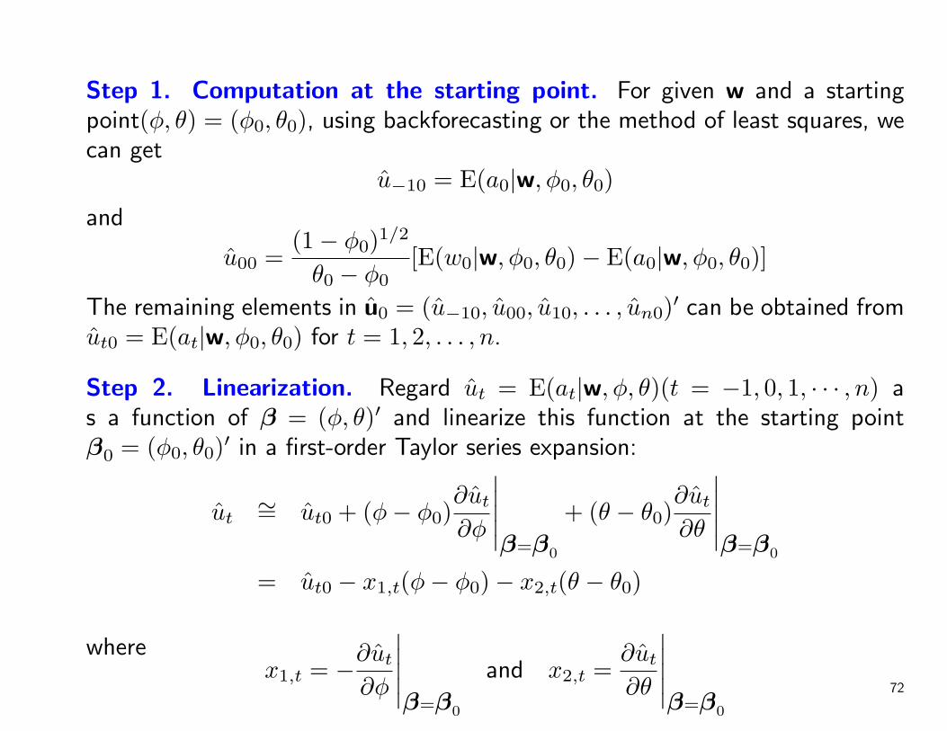
Step 1. Computation at the starting point. For given w and a startingpoint(φ, θ) = (φ0, θ0), using backforecasting or the method of least squares, wecan get
u−10 = E(a0|w, φ0, θ0)
and
u00 =(1− φ0)1/2
θ0 − φ0[E(w0|w, φ0, θ0)− E(a0|w, φ0, θ0)]
The remaining elements in u0 = (u−10, u00, u10, . . . , un0)′ can be obtained fromut0 = E(at|w, φ0, θ0) for t = 1, 2, . . . , n.
Step 2. Linearization. Regard ut = E(at|w, φ, θ)(t = −1, 0, 1, · · · , n) as a function of β = (φ, θ)′ and linearize this function at the starting pointβ0 = (φ0, θ0)′ in a first-order Taylor series expansion:
ut∼= ut0 + (φ− φ0)
∂ut
∂φ
∣∣∣∣∣β=β0
+ (θ − θ0)∂ut
∂θ
∣∣∣∣∣β=β0
= ut0 − x1,t(φ− φ0)− x2,t(θ − θ0)
wherex1,t = −∂ut
∂φ
∣∣∣∣∣β=β0
and x2,t =∂ut
∂θ
∣∣∣∣∣β=β0
72

So we have
ut0 = (x1,t, x2,t)[φ− φ0
θ − θ0
]+ ut
Considering this equation for t = −1, 0, . . . , n, we obtain
u0 = X(β − β0) + u
where u = (u−1, u0, . . . , un)′ and
X =
x1,−1 x2,−1
x1,0 x2,0... ...
x1,n x2,n
The least squares estimate of δ = β − β0 may be obtained from δ =(X ′X)−1X ′u0. Hence we obtain a modified estimator of β as
β1 = β0 + δ
73
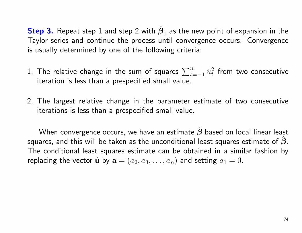
Step 3. Repeat step 1 and step 2 with β1 as the new point of expansion in theTaylor series and continue the process until convergence occurs. Convergenceis usually determined by one of the following criteria:
1. The relative change in the sum of squares∑n
t=−1 u2t from two consecutive
iteration is less than a prespecified small value.
2. The largest relative change in the parameter estimate of two consecutiveiterations is less than a prespecified small value.
When convergence occurs, we have an estimate β based on local linear leastsquares, and this will be taken as the unconditional least squares estimate of β.The conditional least squares estimate can be obtained in a similar fashion byreplacing the vector u by a = (a2, a3, . . . , an) and setting a1 = 0.
74

Standard Errors of the Estimates
Var(β) = σ2(X ′βX β)−1
where the estimate of σ2 is given by
σ2 =S(φ, θ)n
Possible Difficulties in Nonlinear Estimation
• In some cases the convergence to the final estimates can be rather slow. Thiscan be due to poorly chosen Starting values of β0 or to misspecified modelswith too many parameters.
• In some rare case the likelihood function can have more than one maximum,and the estimates can converge to a local maximum rather than a globalone.
75

4.7 Model Checking
• Analysis of residuals at
1. the mean of the residuals should be close to zero,2. the variance of the residuals should be approximately constant,3. the autocorrelation of the residuals should be negligible.
• The sample autocorrelation of the residual
ra(k) =
n∑t=k+1
(at − ¯a)(at−k − ¯a)
n∑t=1
(at − ¯a)2
The standard error of ra(k) is usually approximated as
s[ra(k)] ∼= n−1/2
76
• For small k, the true standard error can be much smaller. In general, thetrue standard error depend on
1. the form of the fitted model,2. the true parameter values,3. the value of k
77

Portmanteau Test
• Under null hypothesis of model adequacy, the large-sample distribution of ra
is multivariate normal and that
Q∗ = nK∑
k=1
r2a(k)
has a large-sample chi-square distribution with K−p− q degrees of freedom.
• For small sample size, this test is quite conservative; that is, the chance ofincorrectly rejecting the null hypothesis of model adequacy is smaller thanthe chosen significance level. The modified test statistics is
Q = n(n+ 2)K∑
k=1
r2a(k)n− k
78
4.8 Examples
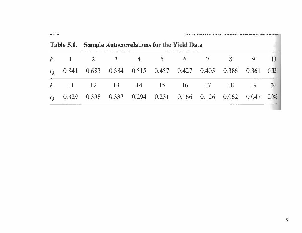
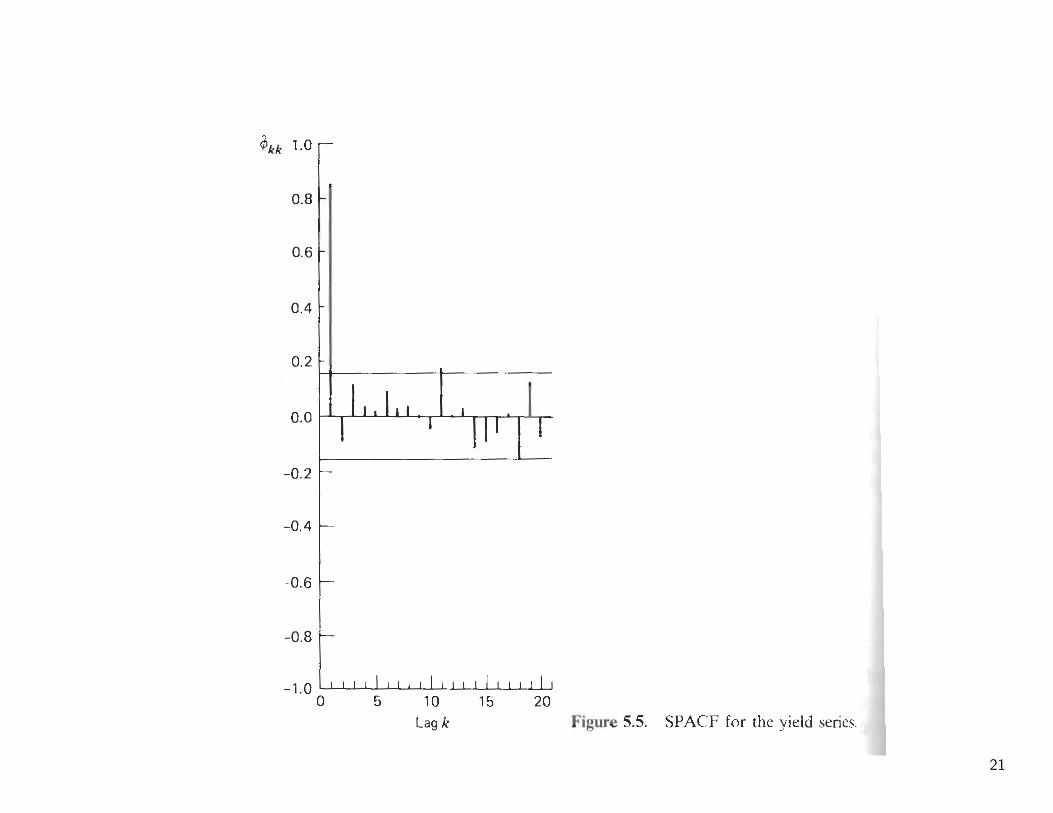
Yield dataThis series consists of monthly differences between the yield on mortgagesand the yield on government loans in the Netherlands from January 1961 toDecember 1973. The observations for January to March 1974 are also available,but they are held back to illustrating the forecasting and updating.
• Figures: Time series plot and SACF
• AR(1) modelzt − µ = φ(zt−1 − µ) + at
The maximum likelihood estimates are
µ = 0.97(0.08), φ = 0.85(0.04), σ2 = 0.024
79

80

• SACF of the residuals
• the Q statistics. Suppose take K = 24. Then
Q = 156×158(
(.09)2
155+
(−.10)2
154+ · · ·+ (.06)2
132
)= 22.4 < χ2
0.05(22) = 33.9
81
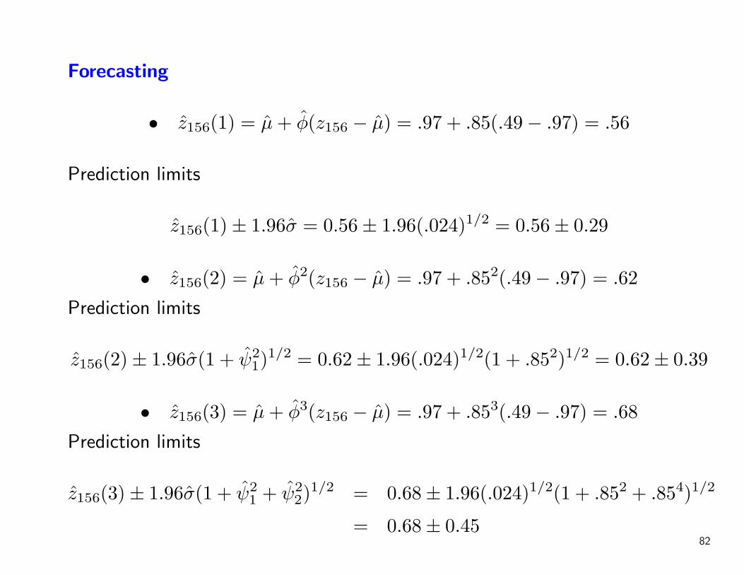
Forecasting
• z156(1) = µ+ φ(z156 − µ) = .97 + .85(.49− .97) = .56
Prediction limits
z156(1)± 1.96σ = 0.56± 1.96(.024)1/2 = 0.56± 0.29
• z156(2) = µ+ φ2(z156 − µ) = .97 + .852(.49− .97) = .62
Prediction limits
z156(2)± 1.96σ(1 + ψ21)
1/2 = 0.62± 1.96(.024)1/2(1 + .852)1/2 = 0.62± 0.39
• z156(3) = µ+ φ3(z156 − µ) = .97 + .853(.49− .97) = .68
Prediction limits
z156(3)± 1.96σ(1 + ψ21 + ψ2
2)1/2 = 0.68± 1.96(.024)1/2(1 + .852 + .854)1/2
= 0.68± 0.4582

Suppose z157 = 0.74 has now become available. Forecasts for z158 and z159are updated according to
• z158 : z157(1) = z156(2) + ψ1[z157 − z156(1)] = 0.62 + .85(.74− .56) = .77
• z159 : z157(2) = z156(3) + ψ2[z157 − z156(1)] = 0.62 + .852(.74− .56) = .81
• The prediction interval for z158 interval for z158 is 0.77± 0.29, and that forz159 is 0.81± 0.39.
83

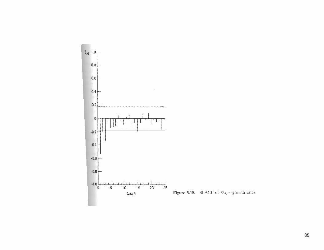
Growth Rates
• Quarterly growth of Iowa nonfarm income from the second quarter of 1948to the fourth quarter of 1978 (N = 123) are shown in Figure 5.8a
• The plot of the series indicates that no variance-stabilizing transformation isnecessary.
• zt is nonstationary and the first difference ∇zt should be analyzed. Thesecond difference is also stationary but would lead to overdifferencing.This is also indicated by the increase in the sample variance [s2(∇zt) =1.58, s2(∇2zt) = 4.82].
• The SACF of ∇zt in Figure 5.11b indicates a cutoff after lag 1. The SPACFin Figure 5.15 shows a rough exponential decay. These patterns lead us toconsider the model
∇zt = θ0 + (1− θB)at
84
85

• The ML estimates and their standard errors are
θ0 = 0.012(.008), θ = 0.92(.04), σ2 = 0.93
• Dropping the insignificant θ0 from the model and reestimating the parametersleads to
θ = 0.88(.04) σ2 = 0.95
• The estimated residual autocorrelations together with their probability limitsare present in Figure 5.16. Q statistic based on the first K = 24autocorrelations (n = 123− 1 = 122)
Q = 122×124(
(−.01)2
121+
(.08)2
120+ · · ·+ (−.09)2
98
)= 20.5 < χ2
0.05(23) = 35.2
Hence we takezt = zt−1 + at − 0.88at−1
as the forecasting model. 86

87

Foreasting
• The predictions z123(`) are described below
z123(`) = z123(1) = z123 − θa123 = 3.38− .88(.718) = 2.75
Note that a123 = .718 is the last residual.
• The estimated variance of the `-step-ahead forecast error is
V [e123(`)] = [1 + (`− 1)(1− θ)2]σ2 = [1 + (`− 1)(1− 0.88)2](.95)
• after a new observation z124 = 1.55 has become available, update the forecast
z124(`) = z123(`+1)+ψ`[z124− z123] = 2.75+(1−0.88)(1.55−2.75) = 2.61
Furthermore, after z125 = 2.93 has become available,
z125(`) = z124(`+1)+ψ`[z125− z124] = 2.61+(1−0.88)(2.93−2.61) = 2.65
88

89

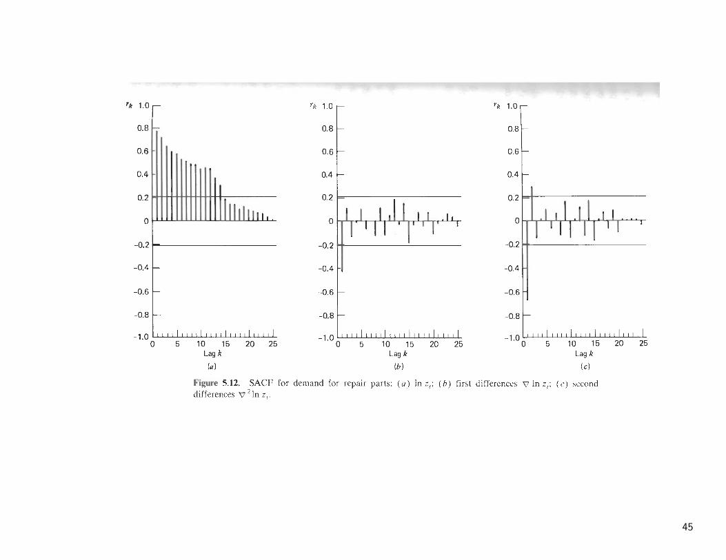
Demand for Pepair Parts This series consists of the monthly demand forrepair parts for a large Midwestern production company from January 1972 toJune 1979 (N = 90). The series is shown in Figure 5.9a.
• A logarithmic transformation need to stabilize the variance and that firstdifferences ∇lnZt are stationary. Further differencing is not necessary sinceit results in an increase in the sample variance [s2(∇zt) = .034, s2(∇2lnzt) =.099]
• The sample autocorrelation and partial autocorrelation are shown in Figure5.12b and 5.17. They indicate a cutoff in the SACF after lag 1 and a roughexponential decay in the SPACF. Thus we consider the ARIMA(0,1,1) model
(1−B)yt = (1− θB)at
where yt = ln zt. The ML estiamtes are
θ = 0.57(.09), σ2 = 0.27
90

91

• A constant θ0 was originally included in the model, but it was found tobe insignificant. The estimated residual autocorrelations , together withtheir probability limits are shown in Figure 5.18. All autocorrelation exceptra(12) are small. The large autocorrelation ra(12) could be due to “seasonalvariation” in the data
• The Q statistic based on the first 24 autocorrelation is given by Q = 37 andis slightly bigger than χ2
0.05(23) = 35.2. This is due mainly to one largeautocorrelation at lag 12.
• It may need to Consider a modification that takes account of the seasonalcomponent.
92

93

Forecasting
• The forecasting model is given in terms of the transformed yt = ln zt. TheMMSE forecasts y(`) and the associated prediction interval c1, c2 for yn+`
can be derive as usual.
• However, to derive the forecasts of original observation zn+` = exp(yn+`),we have to back transform the forecasts and the prediction interval. Theyare given by
zn(`) = exp[yn(`)] and [exp(c1), exp(c2)]
• The forecasts of the transformed series yn+` are MMSE forecasts. However ifthe transformation is nonlinear, as in the case the logarithmic transformation,the MMSE will not preserved for zn(`) = exp[yn(`)].
• Nevertheless, the forecast zn(`) will be the median of the predictivedistribution of zn+`.
94

• For the present example, the prediction y90(`) and the corresponding 95percent prediction limits are given by
y90(`) = y90(1) = y90 − θa90 = 7.864− .57(.234) = 7.731
and
y90(`)±1.96[1+(`−1)(1−θ)2]1/2σ = 7.731±1.96[1+(`−1)(1−.57)2]1/2(.027)1/2.
• Forecasts and 95 percent prediction interval s for y91, y92 and z91, z92 aregiven in Table 5.6.
• The prediction intervals are quite large. This is due partially to the largeuncertainty (σ2) in the past data and partly to the unexplained correlationat lag 12.
95

96