1

4: Speech Compression

Mark Handley

Data Rates Telephone quality voice:

8000 samples/sec, 8 bits/sample, mono 64Kb/s

CD quality audio: 44100 samples/sec, 16 bits/sample, stereo ~1.4Mb/s

Communications channels and storage cost money (although lessthan they used to) What can we do to reduce the transmission and/or storage costs

without sacrificing too much quality?

2

Speech Codec Overview

PCM - send every sample

DPCM - send differences between samples

ADPCM - send differences, but adapt how we code them

SB-ADPCM - wideband codec, use ADPCM twice, once forlower frequencies, again at lower bitrate for upperfrequencies.

LPC - linear model of speech formation

CELP - use LPC as base, but also use some bits to codecorrections for the things LPC gets wrong.

PCM

µ-law and a-law PCM have already reduced the data sent.

Lost frequencies above 4KHz.

Non-linear encoding to reduce bits per sample.

However, each sample is still independently encoded.

In reality, samples are correlated.

Can utilize this correlation to reduce the data sent.

3

Differential PCM Normally the difference between samples is relatively small

and can be coded with less than 8 bits. Simplest codec sends only the differences between

samples.Typically use 6 bits for difference, rather than 8 bits for

absolute value. Compression is lossy, as not all differences can be coded

Decoded signal is slightly degraded.Next difference must then be encoded off the previous

decoded sample, so losses don’t accumulate.

Differential PCMDifference accuratelycodedin 6 bits

max 6 bitdifference

LossyCompression

Code nextdifferenceoff previousdecodedsample

4

ADPCM (Adaptive Differential PCM) Makes a simple prediction of the next sample, based on weighted

previous n samples. For G.721, previous 8 weighted samples are added to make the

prediction. Lossy coding of the difference between the actual sample and the

prediction. Difference is quantized into 4 bits ⇒ 32Kb/s sent. Quantization levels are adaptive, based on the content of the

audio. Receiver runs same prediction algorithm and adaptive quantization

levels to reconstruct speech.

ADPCM

AdaptiveQuantizer

Predictor

++-

Measuredsamples

Transmittedvalues

5

ADPCM Adaptive quantization cannot always exactly encode a difference.

Shows up as quantization noise.

Modems and fax machines try to use the full channel capacity.

If they succeed, one sample is not predictable from the next.

ADPCM will cause them to fail or work poorly.

ADPCM not normally used on national voice circuits, but commonlyused internationally to save capacity on expensive satellite orundersea fibres.

May attempt to detect if it’s a modem, and switch back to regularPCM.

Predictor Error

What happens if the signal gets corrupted while beingtransmitted?

Wrong value will be decoded.

Predictor will be incorrect.

All future values will be decoded incorrectly!

Modern voice circuits have low but non-zero error rates.

But ADPCM was used on older circuits with higher lossrates too. How?

6

ADPCM Predictor Error

Want to design a codec so that errors do not persist.

Build in an automatic decay towards zero.

If only differences of zero were sent, the predictor woulddecay the predicted (and hence decoded) value towardszero.

Differences have a mean value of zero (there are as manypositive differences as negative ones).

Thus predictor decay ensures that any error will alsodecrease over time until it disappears.

ADPCM Prediction Decay

Actual Prediction, p

Decayed Prediction = 0.9p

QuantizedDifferenceTransmitted

7

ADPCM Predictor Error

TransmissionError

Decoderpredictorincorrect

Predictor errordecays away

Sub-band ADPCM Regular ADPCM reduces the bitrate of 8KHz sampled audio (typically

32Kb/s).

If we have a 64Kb/s channel (eg ISDN), we could use the sametechniques to produce better that toll-quality.

Could just use ADPCM with 16KHz sampled audio, but not allfrequencies are of equal importance.

0-3.5KHz important for intelligibility

3.5-7KHz helps speaker recognition and conveys emotion

Sub-band ADPCM codes these two ranges separately.

8

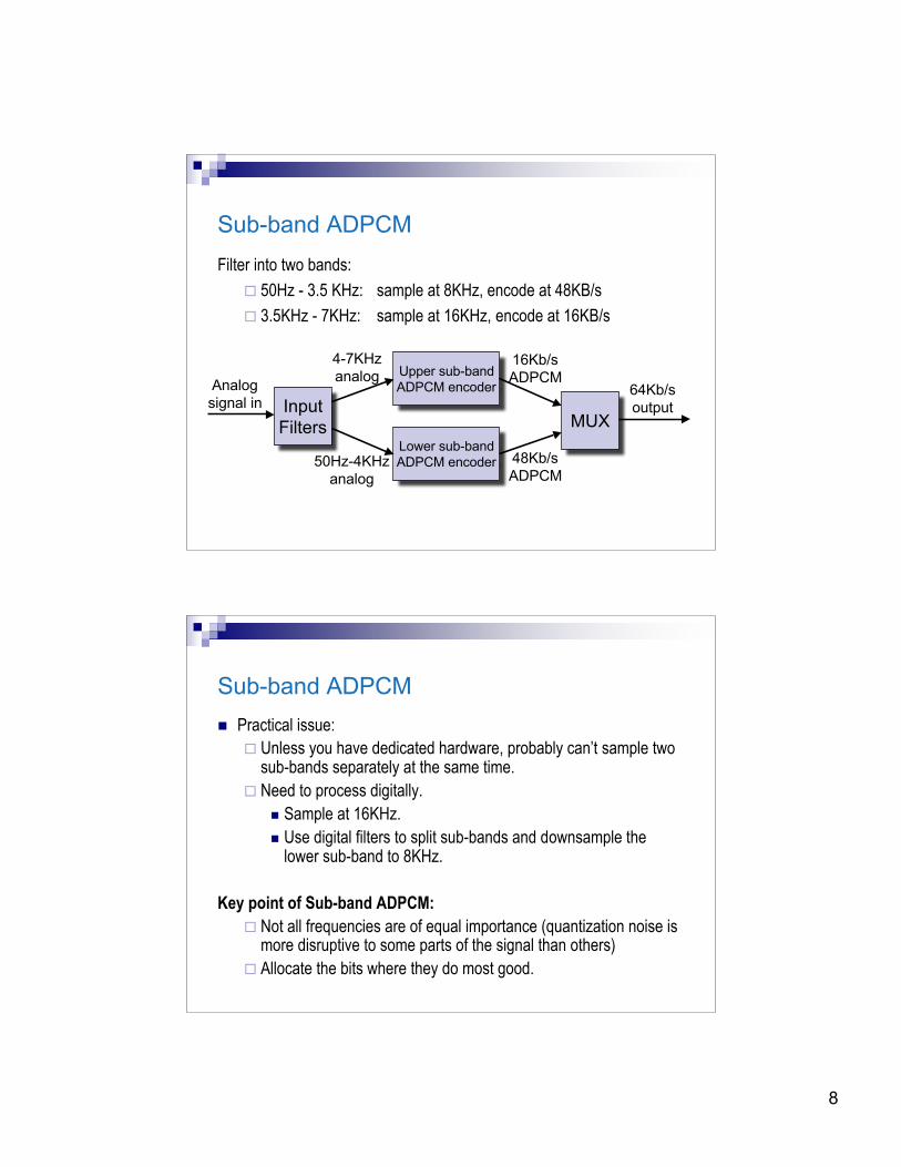
Sub-band ADPCMFilter into two bands:

50Hz - 3.5 KHz: sample at 8KHz, encode at 48KB/s

3.5KHz - 7KHz: sample at 16KHz, encode at 16KB/s

Upper sub-bandADPCM encoder

Lower sub-bandADPCM encoder

InputFilters MUX

Analogsignal in

4-7KHzanalog

50Hz-4KHzanalog

16Kb/sADPCM

48Kb/sADPCM

64Kb/soutput

Sub-band ADPCM Practical issue:

Unless you have dedicated hardware, probably can’t sample twosub-bands separately at the same time.

Need to process digitally. Sample at 16KHz. Use digital filters to split sub-bands and downsample the

lower sub-band to 8KHz.

Key point of Sub-band ADPCM: Not all frequencies are of equal importance (quantization noise is

more disruptive to some parts of the signal than others) Allocate the bits where they do most good.

9

Model-based Coding PCM, DPCM and ADPCM directly code the received audio signal.

An alternative approach is to build a parameterized model of thesound source (ie. Human voice).

For each time slice (eg 20ms):

Analyse the audio signal to determine how the signal wasproduced.

Determine the model parameters that fit.

Send the model parameters.

At the receiver, synthesize the voice from the model and receivedparameters.

Larynx(vocal cords)

Vocal tract(resonance)

Lipsand tongue

Speech formation

Voiced sounds: series of pulsesof air as larynx opens and closes.Basic tone then shaped bychanging resonance of vocal tract.

Unvoiced sounds: larynx heldopen, turbulent noise made inmouth.

10

Linear Predictive Coding (LPC)

Introduced in 1960s.

Low-bitrate encoder:

1.2Kb/s - 4Kb/s

Sounds very synthetic

Basic LPC mostly used where bitrate really matters (egin miltary applications)

Most modern voice codecs (eg GSM) are based onenhanced LPC encoders.

LPC

Digitize signal, and split into segments (eg 20ms)

For each segment, determine:

Pitch of the signal (ie basic formant frequency)

Loudness of the signal.

Whether sound is voiced or unvoiced

Voiced: vowels, “m”, “v”, “l”

Unvoiced: “f”, “s”

Vocal tract excitation parameters (LPC coefficients)

11

LPC Decoder

Voiced orunvoiced

Loudness

Pitch

LPC vocaltract modelcoefficients

LPC Frame

Vocal cordsynthesizer

Unvoicedsynthesizer

GainVocal tract model filter

ReceivedLPCData

Audiooutputsignal

LPC Decoder Vocal chord synthesizer generates a series of impulses.

Unvoiced synthesizer is a white noise source.

Vocal tract model uses a linear predictive filter. nth sample is a linear combination of the previous p samples plus

an error term:xn = a1xn-1 + a2xn-2 + .. + anxn-p + en

en comes from the synthesizer.

The coefficients a1.. ap comprise the vocal tract model, andshape the synthesized sounds.

12

LPC Encoder Once pitch and voice/unvoiced are determined, encoding consists of

deriving the optimal LPC coefficients (a1.. ap) for the vocal tractmodel so as to minimize the mean-square error between thepredicted signal and the actual signal.

Problem is straightforward in principle. In practice it involves:

1. The computation of a matrix of coefficient values.

2. The solution of a set of linear equations.

Several different ways exist to do this efficiently (autocorrelation,covariance, recursive latice formulation) to assure convergenceto a unique solution.

Limitations of LPC Model

LPC linear predictor is very simple.

For this to work, the vocal tract “tube” must not have anyside branches (these would require a more complexmodel).

OK for vowels (tube is a reasonable model)

For nasal sounds, nose cavity forms a side branch.

In practice this is ignored in pure LPC.

More complex codecs attempt to code the residuesignal, which helps correct this.

13

Code Excited Linear Prediction (CELP)

Goal is to efficiently encode the residue signal, improvingspeech quality over LPC, but without increasing the bit ratetoo much.

CELP codecs use a codebook of typical residue values.

Analyzer compares residue to codebook values.

Chooses value which is closest.

Sends that value.

Receiver looks up the code in its codebook, retrieves theresidue, and uses this to excite the LPC formant filter.

CELP (2) Problem is that codebook would require different residue values for

every possible voice pitch. Codebook search would be slow, and code would require a lot of

bits to send. One solution is to have two codebooks.

One fixed by codec designers, just large enough to represent onepitch period of residue.

One dynamically filled in with copies of the previous residuedelayed by various amounts (delay provides the pitch)

CELP algorithm using these techniques can provide pretty goodquality at 4.8Kb/s.

14

Enhanced LPC Usage GSM (Groupe Speciale Mobile)

Residual Pulse Excited LPC 13Kb/s

LD-CELP Low-delay Code-Excited Linear Prediction (G.728) 16Kb/s

CS-ACELP Conjugate Structure Algebraic CELP (G.729) 8Kb/s

MP-MLQ Multi-Pulse Maximum Likelihood Quantization (G.723.1) 6.3Kb/s