4 photoemission from liquids: results and discussion
TRANSCRIPT

42
4 Photoemission from Liquids:
Results and Discussion
4.1 Pure Liquid Water
The electronic structure of liquid water is not well understood even though this property
holds the key to understanding the chemical and physical properties of matter. Furthermore,
the study of the electronic states in hydrogen bonded (H-bonded) systems is of great inter-
disciplinary importance. A well suited technique by which this information may be accessed
is photoelectron spectroscopy [24]. The only valence photoemission experiment from liquid
water reported to date, which extends beyond the top of the valence band [22], was per-
formed with focused HeI (21.2 eV) radiation using a similar microjet setup as in the present
work [28]. With this laboratory photon source the outer three valence orbital energies of
liquid water were measured for the first time, however, on a large background of secondary
electrons [4,26,47]. For the present study the microjet apparatus has been modified for the
use at a synchrotron radiation source (see 3.2.1). This enables for systematic studies of the
dependence of the photoemission spectra on photon energy, flux, and polarization. The wide
tunability of synchrotron radiation allows excitation at maximum photoionization cross sec-
tion, which is particularly advantageous if low-concentration aqueous solutions are examined.
Assessing resonances, e.g. charge-transfer-to-solvent excitation in the case of aqueous ions,
is of great fundamental importance [48, 49, 50]). Furthermore, the use of polarized photons
of tunable energies not only enables to map but also to reasonably interpret photoionization
cross sections.
Here the first full range (inner and outer) valence photoemission spectra of liquid water
will be presented. The photon energy range from 30 to 140 eV enables the investigation of
previously inaccessible electronic structural features. Liquid-specific photoelectron scattering

4.1 Pure Liquid Water 43
1400
1200
1000
800
600
400
200
0
phot
oem
issi
on s
igna
l [ar
b. u
nits
]
-100 -80 -60 -40 -20 0
binding energy [eV]
1b1
3a1
2a11b2
1b1g
2
1'
1
(I) (II) (III)
gas &liquid
hν = 100 eV
Figure 4.1: Photoemission spectrum of pure water obtained after photoexcitation of thewater jet using 100 eV photon energy. The spectrum was optimized for maximum liquid-to-gas-phase intensity ratio (see text). 1b1g refers to the respective gas-phase orbital; the othergas-phase contributions strongly overlap with the liquid features. Labels denote the waterorbitals, single numbers 1, 1’, 2 partly denote the electron energy-loss features (see section4.1.4). The emission between 90 - 100 eV is the low-kinetic energy cutoff region.
processes are addressed, and partial ionization cross sections, dσ/dΩ, of the liquid water
molecular orbitals for some selected photon energies are reported. The role of surface species
and the effect of hydrogen bonding will be discussed.
4.1.1 General Features, Spectral Assignment and Analysis
Fig. 4.1 shows a typical full-range photoemission spectrum from pure liquid water obtained
for 100 eV excitation photon energy (acquisition time was about 30 minutes). The energies
in the figure are binding energies calibrated to the gas-phase water 1b1 orbital 1 ionization
threshold (set to 12.60 eV [51] as discussed below).
Unlike in the case of metal samples where the Fermi energy (EF ) provides an internal
energy reference, in liquids and solutions, energies are related to a reference potential (ref-
1hereafter the 1b1 gas-phase orbital will be denoted 1b1g.

44 4 Photoemission from Liquids: Results and Discussion
erence electrode). In aqueous solutions one typically defines the free energies and enthalpies
of the hydrogen ion, and of the elements in their standard states, as energy zero [52]. This
is technically difficult for the free jet, which may be treated in many respects similarly to
free clusters (which may be of very large size with aggregation states being liquid or solid-
like). In cluster photoemission studies absolute ionization potentials are typically obtained
by calibration using a gaseous species of known threshold energy. Generally not relevant
in cluster studies is the presence of surface potentials caused by oriented surface species,
giving rise to a surface dipole. Whether or not this exists for water is still debated. For the
present case, the 1b1g gas-phase binding energy was chosen as an external energy reference.
Its peak position and width is found to remain constant in the photoemission spectra as the
jet was moved out of the spectrometer acceptance angle by 50 - 100µm. This implies that all
gas-phase water is sampled from the identical potential between the jet and the spectrometer
skimmer, which makes the measured 1b1g energy a convenient and precise reference.
For a more detailed discussion of the photoemission spectrum in Fig. 4.1 it will be useful
to consider the low kinetic energy part (I), the medium range (II), and the valence orbital
region (III) separately. The latter region (III), between ca. 10 - 35 eV binding energy, is
characterized by distinct emission features predominantly arising from the four outer orbitals
of the H2O molecule, 2a1, 1b2, 3a1, 1b1 as introduced in section 2.2. Gas-phase contributions,
denoted by the subscript g in Fig. 4.1, result from the continuous evaporation of the liquid
surface; only 1b1g in labeled since it can be best distinguished (see also Fig. 4.2). Binding
energies and peak width are different for liquid and gas-phase water as will be discussed
in detail below. Broad emission features observed in the center part (II) of the spectrum
(label 2), but also some weaker features at lower binding energy (e.g. features 1, 1’), are in
part assigned to electron energy losses in the liquid. They arise from photoelectrons initially
emitted from the various molecular orbitals of water which subsequently excite the same
transitions known from optical absorption of liquid water [53,54]. This part of the spectrum
also contains rather unspecific electron bulk scattering contributions which give rise to a
broad background.
The assignment of features within the near cutoff region (I) is unclear, and further studies
are required to better understand the issue. In general, this low-kinetic energy region is found
to be extremely sensitive to minor experimental changes (particularly jet position). In fact,
the cutoff features may change considerably from one aligning adjustment to another, at
least, as far as relative intensities are concerned; the energies remain fixed.

4.1 Pure Liquid Water 45
4.1.2 H2O Gas-Liquid Phase Binding Energy Shift
As mentioned in the previous paragraph, quite a large amount of gas-phase water molecules
is detected in the measurement due to the larger focal size of the synchrotron radiation as
compared to the jet diameter. Hence, the analysis of the liquid water properties requires the
separation of the liquid from the gas-phase contributions in the spectra. Fig. 4.2 presents
valence band photoemission spectra of water obtained for 60 eV photons. The abscissa in
gas &liquid
gas
liquid
measured
measured
difference
2a1
1b2
3a1
hν = 60 eV 1b1
10000
8000
6000
4000
2000
0
phot
oem
issi
on s
igna
l [ar
b. u
nits
]
-40 -30 -20 -10 0
binding energy [eV]
1b1g
Figure 4.2: Photoemission spectra sampled for maximum liquid signal (top), from gas-phasewater sampled > 100 µm aside the liquid jet (center), and difference spectrum (bottom),obtained for 60 eV photon energy. Labels denote the water orbitals. From the top spectruma Shirley-type background [55] was subtracted.
the figure is the electron binding energy relative to vacuum and the axis is fixed with respect

46 4 Photoemission from Liquids: Results and Discussion
8000
6000
4000
2000
0
phot
oem
issi
on s
igna
l [ar
b. u
nits
]
-40 -30 -20 -10
binding energy [eV]
2a1
1b2 3a1
1b1g 1b1
(1)
(2)
(3)
(4)
hν = 60 eV
Figure 4.3: Gas-phase subtraction from the measured (maximum liquid) photoemissionspectrum. (1) Photoemission spectrum (background subtracted) obtained for 60 eV pho-ton energy. (2) and (3) exemplify incorrect subtraction, corresponding to too little or toomuch gas-phase subtraction (as judged by the 1b1g peak or dip, respectively). (4) Optimumdifference spectrum.
to the 1b1g (gas phase) molecular orbital (see 4.1.1).
The center spectrum in Fig. 4.2 is a pure gas-phase spectrum (obtained by moving the
jet aside relative to the spectrometer entrance by some hundred microns), and the top
spectrum displays the measured liquid spectrum characterized by a maximum liquid-to-gas
phase intensity ratio. Qualitatively similar results were obtained for other photon energies.
The labels in the figure denote the molecular orbitals (MOs) of the water molecule (see
section 2.2).
Since identical binding energies and peak widths are obtained for the gas-phase lone pair
orbital, 1b1g, for both the (maximum) liquid and the gas-phase photoemission spectra, one
may subtract, with proper scaling of the relative intensities (as illustrated in Fig. 4.3), the gas
from the liquid spectrum. The difference spectrum, bottom curve in Figs. 4.2 and 4.3, is our
best experimental approach to the valence photoemission spectrum from pure liquid water.
The main difference between the pure liquid and the pure gas-phase spectra is a binding
energy shift of the liquid water orbitals to lower values, accompanied by considerable liquid

4.1 Pure Liquid Water 47
5000
4000
3000
2000
1000
0
phot
oem
issi
on s
igna
l [ar
b. u
nits
]
-40 -30 -20 -10
binding energy [eV]
2a1
1b2 3a1
1b1
60 eV
80 eV
100 eV
-12 -11 -10 -9
1b1
Figure 4.4: Gas-phase subtracted photoemission spectra for 60, 80 and 100 eV. Constantpeak positions are indicated by vertical lines. The inset is a zoom into the low binding energyonset of the liquid-water 1b1 emission, showing the ionization threshold.
peak broadening as summarized in Table 4.1. The values in the table result from Gaussian
peak fitting averaged over a number of spectra. No dependence of the excitation photon
energy (60, 80, 100 eV) on both width and binding energy has been observed. Representative
gas-phase subtracted photoemission spectra for 60, 80 and 100 eV are presented in Fig. 4.4.
The spectra are normalized to the 1b1 liquid water feature. Constant peak positions are
indicated by vertical lines. The differences of the relative photoemission intensities, as a
function of the photon energy, are discussed in section 4.1.3, which is concerned with the
relative partial photoionization cross section of liquid water in detail.
Fig. 4.5 is a presentation of the spectral analysis (60 eV photon energy), which was used
to derive both peak energies and widths, shown in Table 4.1. Prior to subtracting the
measured gas-phase spectrum (center Fig. 4.2) from the measured maximum liquid spectrum
(top Fig. 4.2) a background (Shirley-type [55]) was subtracted from the latter. The result
is shown in Fig. 4.5 along with the corresponding Gaussian peak fits. As will be discussed
below (4.1.4), in addition to the main peak for the 2a1 feature, two further peaks of identical
height and width on either side of the main peak were introduced. Also for fitting the 3a1

48 4 Photoemission from Liquids: Results and Discussion
3000
2000
1000
0
phot
oem
issi
on si
gnal
[arb
. uni
ts]
-40 -30 -20 -10
binding energy [eV]
2a1
1b2 3a1
1b160 eV
Figure 4.5: Representative Gaussian peak fitting shown for a photoemission spectrum ofpure liquid water (here obtained for 60 eV photon energy). The extra peaks required forfitting the 2a1 feature account for distinct electron energy losses. A double-peak structurehas been assumed for the 3a1 feature in order to account for possible Davydov splitting.
feature two peaks were used, however, for a different reason (see 4.1.3).
The observed differential gas-liquid peak shifts are 1.72 ± 0.16, 1.46 ± 0.06, 1.34 ± 0.12,
and 1.45 ± 0.05 eV for the 2a1, 1b2, 3a1, and 1b1 orbitals, respectively (see Table 4.1). As the
statistical error is smaller than the mean relative energy differences, the observed differential
shifts are considered to be significant. Notice that simple Gaussian fitting neglects possible
differential shifts due to altered vibronic spectra of liquid water as a consequence of modified
molecular structures.
Origin of gas-liquid energy shift. The observed gas-liquid peak shifts of water are the
net result of different contributions: electronic polarization, surface dipoles, and H-bonding
induced orbital changes. The two former contributions would be expected to make up for
the observed mean shift, which is supposed to be identical for all orbitals. The polarization
term refers to the fact that the emitted photoelectron may sense the fast (on the time scale
of the photoemission process) polarization screening by the (liquid) environment around the
photo-generated charge. Such a final state effect is common in photoemission of condensed
molecular systems, where electron binding energy shifts are on the order of 1 - 2 eV just as
in the present case [57]. For liquids, (fast) polarization screening may be treated similarly
to the static electronic polarization of the solvent [25]. Traditionally, such shifts are derived

4.1 Pure Liquid Water 49
Orbital Eg [eV] Eaq [eV] FWHM [eV] FWHM [eV] Shift(g-l) broadening
MOi Gas Liquid Gas Liquid [eV] factor (liq)
(this work) (this work) (this work)
1b1 12.60 11.16(4) 0.30(1) 1.45(8) 1.45(5) 4.03
0.09 a
3a1 14.84(2) 13.50(10) 1.18(2) 2.52(10) 1.34(12) 2.14
14.85 a 1.03 a
1b2 18.78(2) 17.34(4) 1.74(2) 2.28(8) 1.46(6) 1.31
18.76 a 1.62 a
2a1 32.62(10) 30.90(6) 2.82(4) 3.30(6) 1.72(16) 1.17
32.52 a 2.34 a
Table 4.1: Experimental electron binding energies (Eg, Eaq), peak widths (FWHM) andexperimental gas-to-liquid energy shifts of the four H2O (gas and liquid) valence orbitals.For comparison respective literature high-resolution data for gas-phase water are also shown:a [56]
from the Gibbs free energy of solvation 2 based on the Born equation [12]:
∆GBorn = − Z2e2
8πε0R(1− 1
ε) . (4.1)
The model assumes electronic polarization (typically static polarization) of a continuum
solvent around an ion with charge Ze and radius R; ε0 is the vacuum permittivity and
ε is the relative permittivity of the solvent. For the case of photoemission, only the fast
process contributes, while the rearrangement of the solvation structure can be neglected
[25]. Therefore, the optical macroscopic relative permittivity of liquid water, εopt, is used to
describe the response. This accounts for the electronically polarized but not for reoriented
surrounding in terms of nuclear positions of water molecules. In section 4.2.5 it will be
seen that for aqueous ions, on the other hand, the slow (static) response, εst, is the most
important (see also Fig. 4.38).
Since the solvation process for any solute is its transfer from a fixed point in vacuum to
a fixed point in solution, one can obtain the Gibbs free energy of solvation of an ion from
the difference of the Gibbs energy of the aqueous and of the gaseous ion. As mentioned in
2Terminology varies considerably: Gibbs free energy, Gibbs function or free enthalpy [16,58]. In Ref. [58]
one also finds: ’The partial molar Gibbs free energy G is equivalent to the chemical potential µ’.

50 4 Photoemission from Liquids: Results and Discussion
section 2.3 (see Born cycle diagram; Fig. 2.6), ∆GBorn (equation 4.1) needs to be evaluated
for both the initial and the final state, i.e. for the neutral and the ionized liquid, respectively
(see also section 4.2.5). The ion electron binding energy difference between liquid and gas
phase, which equals the liquid phase shift, is obtained by EBornaq − Eg = ∆G. Here Eg
and Eaq denote the respective gaseous and aqueous electron binding energies, and ∆G =
∆GBornf −∆GBorn
i accounts for the ionization state of the system before (initial) and after
(final) photoionization. It is noted that even though the Born model is primarily applied
for solvated ions (see section 4.2.5), formally the concept may be applicable for the pure
solvent as well. The main difference is the absence of an initial hydration shell for the latter
case, and hence orientational contributions to the gas-liquid phase shift are of no concern.
As we will see below, this also explains the considerably smaller energy shifts observed for
pure water as compared to aqueous ions. Using an effective (theoretical) solute cavity radius
Reff = 2.24 A of pure water [14], and an optical permittivity εopt ' 1.78 [8], one obtains
−∆GBorn = 1.41 eV from equation 4.1 (for removing the outermost electron). The good
agreement with the experimental shift is attributed to the small size of the water molecule
as this allows for the assignment of a well-defined cavity radius [25]. On the other hand,
as no structural details are taken into account in this continuum model, this value only
constitutes a rough estimate. The limits of the model will be discussed in further detail in
section 4.2.5.
As mentioned above, polarization screening is not the only possible contribution to the
measured shifts. The surface potential of water, due to oriented surface dipoles, would also
cause a spectral shift in photoemission. The magnitude of this potential is not well known,
but it is likely to be some ten mV. With a voltaic cell the surface potential of pure water was
determined to be about 25mV [59]. Depending on the detailed structure of the water-vacuum
interface, especially the density and the orientation of the intrinsic water dipole moments at
the surface, the electrostatic contributions to the surface work function could range from a
few meV 3 (moments parallel to the surface) up to approximately 1 eV (assuming the O-H
bond being perpendicular to the surface, which, however, seems unlikely).
3It is interesting to compare this number with surface structural data obtained by vibrational spec-
troscopy of water at the vapor/water interface [60]. With the free OH pointing out of the liquid, the bonded
OH must point into the liquid (H-bonded). In fact the permanent dipoles of water are suggested to lie close
to the surface plane [60]. The result indicated that the surface density of this species is more than 20% of
a full monolayer, i.e. n > 2.7× 1014 cm−2. Based on these data, assuming the OH bond being perpendicular
to the water surface, one obtains m⊥ = 1.13 D for the normal component of the surface dipole per water

4.1 Pure Liquid Water 51
Understanding differential binding energy shifts requires some theoretical treatment of
the electronic structure of bulk liquid water which, however, generally suffers from an in-
adequate description of the H-bonding and the relevant interaction potentials [3]. Most of
present electronic (band) structure theories of liquid water are crude, besides, only a few
reports are available [62,63,64]. In fact, band energy positions of liquid water are still subject
of continuing debate [65] with the only consensus being the assignment of 10.06 eV below
the vacuum level for the top of the valence band [65, 66]. This value has been known from
rather early threshold photoemission experiments using photon energies near 10 eV [22]. A
value of about 9.9 eV is obtained for the onset of the 1b1 photoemission feature as shown in
the inset of Fig. 4.4. The water ionization threshold energy, including the possibility of au-
toionization contributions in the context of the generation of solvated electrons, is discussed
in Refs. [22, 67].
Very recently, evidence for water molecular orbital structural changes, if the water
molecule is brought into the liquid environment, was reported both by experiment [2, 9]
and theory [3]. In the latter study it was found that, with respect to the case of the iso-
lated molecule, in bulk water the lone pair orbitals are pulled out due to the formation of
H-bonds, while the covalent bond orbitals are pulled in. These changes correlate with the
existence of distinct molecular species, characterized by varying H-bonding, and also with an
increase of the average O-H bond length. This increase can be viewed as a charge-transfer
process in which the hydrogen atoms lose electrons in favor of the oxygen atoms [3]. As a
consequence, in the liquid the electronic charge is more spherically distributed around the
oxygen atoms [3]. Regarding the orbital energies, no obvious correlation between measured
binding energy shifts and theoretically expected trends [3] could be found. Presumably, this
reflects the multiple contributions to the experimental gas-liquid binding energy shift. To
make this point more clear, photoemission from liquid water is a much more complex task
than for typical gaseous or solid samples. This is partly due to the nature of volatile liquids;
it is simply impossible to separate liquid water from its vapor. Another difficulty is how to
molecule, which is an upper bound. Using the Helmholz equation [61]:
∆Φ =enm⊥
εrε0, (4.2)
with εr = 1 (in order to account for the liquid/vacuum interface), we obtain 1.14 eV for the work function
change. This value might seem large, but one has to realize that the OH bond being fully perpendicular to
the surface is a rather unrealistic assumption [60]. Clearly, for dipole moments almost in the surface plane
smaller values for ∆Φ would be obtained (some ten meV).

52 4 Photoemission from Liquids: Results and Discussion
account for the role of the surface potential. As mentioned above, this issue still needs to
be understood, and consequently, also for the present results, the mean contributions to the
energy shift by surface dipoles cannot be quantified. The interesting result, at this point, is
the fact that differential contributions in addition to polarization screening and surface po-
tential were identified, which reflects the effect of H-bonding on water’s electronic structure.
In section 4.1.3 it will be argued that the influence of H-bonding is also responsible for the
peculiar behavior of the H2O 1b2 orbital photoionization cross section measured here. In fact
the photoionization cross section appears to be a more sensitive tool for probing differences
of the electronic structure of water in its different aggregation states.
Peak broadening. Peak widths of all valence orbitals are increased as compared to
the gas phase, however, not by the same relative amount as presented in Table 4.1. For
comparison, the table also contains the widths of the respective gas-phase water orbitals of
both the present spectra and high-resolution photoemission studies [56] (see Fig. 4.6). The
latter correspond to the widths of the envelope of the vibrational structure of the bands,
which is not resolved in the present experiment. The differential broadening of the liquid
-22 -20 -18 -16 -14 -12 -10
1b23a1
1b1
40x103
30
20
10
0
phot
oem
issi
on s
igna
l [ar
b. u
nits
]
-60 -50 -40 -30 -20 -10 0
binding energy [eV]
1b22a1
3a1
1b1hν = 100 eV
11'
Figure 4.6: High-resolution photoemission spectra of gas-phase H2O [56] obtained for 100 eVphoton energy. The photoemission spectra in the inset, covering a shorter energy range, wasmeasured at increased resolution. Arrows indicate features the origin of which is discussedin the text.

4.1 Pure Liquid Water 53
Orbital Eice [eV] Eaq [eV] FWHM [eV] FWHM [eV]
MOi Ice Liquid Ice Liquid
(this work) (this work)
1b1 12.3 c,d 11.16(4) 1.3 g 1.45(5)
11.8 e 1.28 h
3a1 14.2 c,d 13.50(10) 2.5-3.0 g,h 2.52(10)
1b2 17.6 c,d 17.34(4) 2.0 g 2.28(8)
18.0 e 1.82 h
2a1 31.0 f 30.90(6) 3.3 f 3.30(6)
Table 4.2: Experimental electron binding energies (Eaq) and peak widths (FWHM) of thefour H2O valence orbitals obtained from liquid water photoemission spectra. For comparisonrespective data for ice (Eice, FWHM) are shown: c [69], d [7], e [70], f [71], g [72], h [73]
with respect to the gas phase peaks is by a factor of about 1.17, 1.31, 2.14 and 4.03 for the
2a1, 1b2, 3a1, and 1b1 orbital, respectively. Hence, also the widths of individual orbitals are
differently affected as the water molecule is brought into the liquid environment. Most likely,
the main broadening effect can be associated with the presence of a distribution of different
local environments (and hence slightly different energies) of a given water molecule within
the H-bonding network [9]. Particularly, structural network differences of surface vs. near-
surface water, located within the first few layers, may be important in our experiment. Also
lifetimes of electronic states are likely to differ for surface water, which could be another
source of peak broadening. Finally, it is pointed out that the measured 1b1 (liquid) peak
width well agrees with the conduction bandwidth of water, 1.45 ± 0.25 eV [68], which would
suggest that the measured value is close to the true intrinsic bandwidth.
The narrowest peak width is observed for the 1b1 orbital of the liquid-water molecule,
which is also true for gas-phase water. In the latter case the small width results from the
non-bonding character of this orbital. Similarly, in liquid water the 1b1 contribution to H-
bonding would seem the smallest among the valence orbitals. In the next section it will
be shown that the broadening of the 3a1 feature correlates with an apparent signal loss as
compared to the gas phase. In fact, this feature needs special consideration as it seems to be
split in two components, which points to the importance of this orbital in H-bonding. Notice
that the 3a1 orbital was predicted to lose its original character [1] as mentioned above.
Liquid water versus ice. As both the liquid and the solid H2O phase structures are

54 4 Photoemission from Liquids: Results and Discussion
governed by hydrogen bonding, the question to be asked is how similar the water and the
ice surfaces actually are. The differences appear to be small as the overall spectral features
of liquid and ice photoemission are very similar as shown in Fig. 4.10 (see next paragraph).
Hence, no clear answer to this question can be given. Yet, electron binding energies tend
to be slightly larger in ice, by about 0.1 - 1.0 eV. The corresponding values, obtained for
adsorbed H2O multilayers on single-crystal surfaces [69, 72, 73, 74, 75] or for crystalline ice
[70,71], are presented in Table 4.2. Regarding the 3a1 and 1b2 orbitals, the observed energy
shifts would be qualitatively consistent with the expected larger O-O and O-H distances
in liquid water [71]. Notice that the 3a1 orbital also plays a central role in bonding water
to single-crystal surfaces (as it does in H-bonding mentioned above), specifically in binding
water to cation sites on oxides [7]. Moreover, the relative orbital binding energy shifts for
adsorbed water correlate with the strength of the adsorption bond to the cation site on the
oxide; consequently the effect decreases for subsequent water layers. The dependence of the
differential binding energy shifts on the nature of the substrate has been evaluated in detail
in Ref. [7].
Linewidth differences for liquid water and ice cannot be discerned. Quantifying this ef-
fect is difficult since experimental widths for ice have generally not been explicitly reported.
Hence, widths for ice, as shown in Table 4.2, are based on a rather crude analysis of pub-
lished spectra (see caption in Table 4.2 for references). Notice also that the assignment of
precise values to the widths is complicated due to substantial band overlap, which partic-
ularly applies to the 3a1 feature. In addition, the latter feature seems to even split in two
components in solid ice. Splitting of this feature in solid ice has in fact been considered
earlier, even though the data were not conclusive [57, 72, 75]. In Ref. [57] it was argued
that for H2O multilayers the broadening, attenuation, and splitting of this peak arise from
H-bonding. For the present case it is also not possible to resolve if this feature is split in two
components for liquid water. Even though it is unclear how to accurately account for both
peak energy and width of this feature, for the analysis of the present photoemission spectra
a two-component feature (of identical peak height and width) consistent with Davydov split-
ting 4 was assumed. This is demonstrated in Fig. 4.5, which represents a typical fit to our
data, and from which the values presented here are inferred. Similarly, in a theoretical study
of the electronic band structure of cubic ice, the splitting of the 3a1 orbital was interpreted
4A given molecular energy level may split into as many components as there are translationally inequiva-
lent molecules per unit cell [76]. This splitting is in addition to the level splitting produced by the interaction
energy between two adjacent identical molecules.

4.1 Pure Liquid Water 55
-80
-70
-60
-50
-40
-30
Li+(1s)
E (eV)
Li+(1s)
Na+(2p)
Na+(2s)
Na+(2p)
Na+(2s)
K+(3s)
K+(3p)
K+(3p)
Cs+(4d)
Cs+(4d)
Cs+(5p)
aq.
aq.
aq.
aq.
aq.
-70
-60
-50
-40
-30
-20
-10
Cl-(3p)
Cl-(3p)
aq. aq. aq.Br-(3d)
Br-(3d)
Br-(4p)
I-(5p)
I-(5p)
I-(5s)
I-(4d)
I-(4d)
-80
-70
-60
-50
-40
-30
Li+(1s)
Na+(2p)
Na+(2s)
Cs+(5p)
Cs+(4d)
K+(3p)
K+(3s)
Li+(1s)
Na+(2p)
Cs+(4d)Cs+(4d)
K+(3p)
Na+(2s)
gas phase liquid
-30
-20
-15
gas phase liquid ice
1b1
3a1
1b2
2a1
E (eV)
-35
Figure 4.7: Comparison of electron binding energies of water orbitals in liquid, gas-phase,and ice. Binding energies for liquid and gas-phase were determined in the present work (seeTable 4.1). Ice values were obtained from the literature (see Table 4.2).
to also arise from the Davydov interaction between two molecules of different orientation
in the unit cell [71]. Considerable energy level splitting has been also found in very recent
calculations of the influence of H-bonding on the local electronic structure [1].
In conclusion, noticeable parallels are found between the bonding of water in bulk water
(H-bonding) as compared to water binding to single crystals. This particularly refers to
the behavior of the water 3a1 orbital. Yet, there might be small binding energy differences,
reflecting electronic structural differences for H-bonded water and ice. Certainly further
experiments, including photoemission from condensed water films, would be useful.

56 4 Photoemission from Liquids: Results and Discussion
4.1.3 Relative Partial Photoionization Cross Sections of Liquid
Water
In the following section the relative partial photoionization cross sections of liquid water
will be discussed. The results for the measured differential relative photoionization cross
sections, dσi/dΩ, are displayed in Table 4.3 for the four water orbitals. Shown are the raw
peak integrals (normalized to the 1b1 liquid feature) as obtained by fitting each (pure liquid)
photoemission spectrum to Gaussians. No attempt was made to determine absolute partial
ionization cross sections in the present work.
The indicated scatter of the values was inferred by comparing different fitting procedures,
i.e. with constant vs. variable peak width at fixed (averaged) orbital binding energy. The
errors obtained for the same method, but evaluating different spectra, are smaller than the
ones given in Table 4.3. Rather large deviations for the 3a1 orbital, in the case of liquid
water, arise from the strong spectral overlap with the 1b1 orbital. The relatively large
uncertainty in determining the 2a1 integral arises from the difficulty to properly account for
the low and high-energy wings of this feature (see sections 4.1.1 and 4.1.4). For reference,
the corresponding gas-phase integrals are displayed in the table as well. These latter values
can be determined more accurately due to both the strongly reduced background and the
fact that the peaks do not overlap.
Orbital Intensity liquid Intensity gas phase
MOi 60 eV 80 eV 100 eV 60 eV 80 eV 100 eV
1b1 1.00 1.00 1.00 1.00 1.00 1.00
3a1 0.96(6) 0.99(6) 1.06(6) 1.16(3) 1.23(3) 1.12(3)
1b2 0.83(3) 0.76(3) 0.80(3) 1.68(4) 1.67(4) 1.50(4)
2a1 0.43(8) 0.38(8) 0.36(8) 0.41(10) 0.40(10) 0.36(10)
Table 4.3: Experimental liquid and gas-phase relative photoemission intensities (as mea-sured) of the four H2O valence orbitals for three photon energies 60, 80, 100 eV, obtained inthe present study.
From Table 4.3 significant differences with respect to the relative intensities for liquid and
gas-phase water can be observed (see Fig. 4.8a). Relative intensity changes are particularly
noticeable for the 1b2 orbital, which is about 50% smaller than in the gas phase. For 3a1
the effect is smaller, but difficult to be quantified due to the peak splitting (see above); the
relative decrease is no more than 10%. This behavior seems to be one of the keys to the

4.1 Pure Liquid Water 57
1.5
1.0
0.5
0.0
mea
sure
d in
tens
ities
[ar
b. u
nits
]
H2Ogas phaseliquid
H2O orbitals
2a1 1b2 3a1 1b1
hν = 60 80 100 eV
1.5
1.0
0.5
0.0
mea
sure
d in
tens
ities
[ar
b. u
nits
]
D2Ogas phase
liquid
D2O orbitals
2a1 1b2 3a1 1b1
hν = 60 80 100 eV
Θ = 90°
Θ = 90°
a)
b)
Figure 4.8: Measured differential partial photoionization cross sections, dσi/dΩ, of waterorbitals for liquid H2O and D2O, obtained for 60, 80, 100 eV photon energies. Data arenormalized to the 1b1 value. The H2O data were taken from Table 4.3, and the data for D2Ofrom Table 4.6. Photoelectron detection is perpendicular to the light polarization vector(Θ = 90 ).

58 4 Photoemission from Liquids: Results and Discussion
Orbital σi liquid σi gas phase
MOi 60 eV 80 eV 100 eV 60 eV 80 eV 100 eV
1b1 1.00 1.00 1.00 1.00 1.00 1.00
3a1 0.69 0.84 0.96 0.84 1.03 1.02
1b2 0.39 0.36 0.41 0.79 0.80 0.78
2a1 0.46 0.47 0.51 0.44 0.50 0.51
Table 4.4: Relative partial photoionization cross sections σi of H2O calculated using datafrom Table 4.3 and 4.5 (gas-phase βi) in equation 4.4.
variation of the water molecular orbital structure due to H-bonding. On the other hand,
oriented species at the water surface might contribute to cross section changes as well. Both
aspects will be discussed in the following.
Photoionization cross section measurements in the gas phase (statistically oriented mole-
cules) are usually performed at the magic angle [43] (see section 3.1.3) as this allows for
determining cross sections independent of the experimental geometry. However, from the
measured quantity dσi/dΩ, obtained for a given geometry, the integrated cross sections
(relative partial photoionization cross sections) σi may be calculated using [41,51] (for linear
polarization):dσi
dΩ=σi
4π[1 +
βi
4(1 + 3P1cos2Θ)] . (4.3)
It will be shown below that this presentation, in fact, better suits the interpretation of the
origin of the different cross sections between liquid and gas-phase water. In equation 4.3,
βi denotes the energy-dependent asymmetry (anisotropy) parameter (2 ≥ β ≥ -1), P1 is
the Stokes parameter (degree of linear polarization), and Θ measures the angle between
the direction of the ejected electron and the polarization of the incident light. For this
experiment P1 = 1 (synchrotron light is 100% horizontally polarized), Θ = 90 (detection
normal to the polarization) and thus from the equation 4.3 one obtains:
σi =4π
(1− βi
2)(dσi
dΩ) . (4.4)
For liquid water one then has two unknown parameters for each orbital; notice that the
βi are known for gas-phase water only. As the present experimental setup did not allow for
measuring photoemission spectra from the liquid jet either at the magic angle or for another
geometry different than depicted in Figs. 3.7 and 3.10, the corresponding βi for liquid water

4.1 Pure Liquid Water 59
Orbital βi liquid βi gas phase
MOi 60 eV 80 eV 100 eV
1b1 — 1.53 1.58 1.59
3a1 — 1.35 1.50 1.55
1b2 — 1.00 1.12 1.21
2a1 — 1.56 1.66 1.71
Table 4.5: Anisotropy parameters βi of gas-phase H2O [51] used in equation 4.4. Data forliquid water are not available.
could not be determined here. Consequently, σi can be calculated for the gas-phase spectra
only; gas-phase βi were taken from Ref. [51] (see Table 4.5). The corresponding plot of
σi for gas-phase water, for the four valence orbitals, is presented as an inset in Fig. 4.9 for
three different photon energies. Values are normalized to σ1b1 ; both sets of gas-phase data
agree well. The main figure (Fig. 4.9) displays calculated σi for liquid water, where the
corresponding dσi/dΩ values together with gas-phase βi have been used in equation 4.4. As
noticed above the relative cross sections σ1b2 (and σ3a1) are found to be smaller. The decrease
is by about 50% (and 10%, respectively), for liquid water. However, with βi for the liquid
being only approximate, the observed changes might principally result from the variation of
σi as well. On the other hand the effect of βi would seem more important, because βi not
only depends on the amplitude but also on the phase shift of the outgoing partial electron
waves. Then, within our simple model, according to equation 4.4, the σ1b2 decrease in Fig. 4.9
can be attributed to a smaller β1b2 for the liquid than for gas-phase water. Apparently the
difference of β1b2 as compared to the other βi, in the gas-phase case 5, is even enhanced in
5Notice that here the change of the β1b2 value was interpreted in terms of a decrease for liquid water. It
is not clear, however, if rather β for the other orbitals decreases or possibly all values change. The answer
to that is difficult as no photoemission investigations of the angular distribution from liquids exist. It is
important to realize that for photoionization of liquids (or solids) photoelectrons experience considerable
inelastic scattering, which reduces the anisotropy of the angular distribution. This may be associated with
a decrease of β. The effect would depend on the probing depth and thus on the photon energy and on the
experimental geometry. In section 4.2.1 it will be shown that considerably intense s photoemission lines can
be observed in the present experiment. This contradicts the expectations for pure atomic s photoionization,
i.e. β = 2, in which case no emission intensity would be detected in the direction perpendicular to the
polarization vector of the synchrotron light (see Fig. 3.5). This shows the importance of determining β
values for liquids using a suitable experimental setup.

60 4 Photoemission from Liquids: Results and Discussion
the presence of H-bonding. In fact this quantity will change if the orbital structure changes.
The reason for the small β1b2 in the gas phase is related to the strong bonding character of
this orbital [51]. As mentioned above, H-bonding affects the covalent bond orbitals causing
a more spherical distribution of electron charge around the oxygen atom [3]. Perhaps this
decreases β1b2 even more for liquid water.
These results show that apparently the relative photoionization cross section is a sensi-
tive probe of water’s molecular changes in the liquid environment which otherwise are very
difficult to be accessed experimentally. Notice that the geometry being used in the present
photoemission experiments (Fig. 3.10) enables the detection of β changes. Specifically, at Θ
= 90 the electron emission probability is about 50% smaller for β = 1.5 than for 1.0.
Possible surface-specific contributions to the cross-sectional behavior will be considered
in the following. This aspect relates to the very surface sensitivity of photoemission for
photoelectron kinetic energies on the order of 20 - 120 eV, which is about the range of the
present experiment. Since the electron mean free path, λe, should be similar for the solid
and the liquid phase, the information depth accessed for pure liquid water is about 2 - 4
layers (see Fig. 3.4), which corresponds to about λe = 1nm assuming the size of a water
molecule being ca. 0.3 nm (see section 4.1.2). Experimental mean free paths for liquid water
have been reported for considerably lower kinetic energies only. The value obtained for 0.1 -
2.0 eV electrons, injected in water, is λe = 3 - 4 nm (or 10 - 15 monolayers of water), which
seems somewhat small according to Fig. 3.4. For low-density amorphous ice theory predicts
values of about 3 - 5 nm for 1 - 20 eV electrons [77], which better agrees with the present
assumption.
The liquid-water surface is assumed to be hydrogen terminated with one free OH project-
ing into the vapor [60]. Also for adsorbed water, for instance on metal surfaces, the first two
layers of water molecules are arranged similarly to the molecules in the most dense layer of
ice [78]. In this structure the higher-lying H2O molecules have one OH bond oriented along
the surface normal and contribute one H atom to the hydrogen bonding network (compare
above discussion on oriented H2O on the liquid water). Notice that for liquid water the OH
axis pointing into the vacuum is likely to be sufficiently inclined towards the surface in order
to stabilize the dipoles within the water surface plane (see discussion footnote, page 50). For
adsorbed water the OH bond may be oriented more upright with respect to the surface. It
then appears feasible that the relative photoemission intensity of a given orbital may vary
based on symmetry arguments and orientational effects. Relative photoemission intensity
differences of the outer valence band orbitals, 1b2, 3a1 and 1b1, have indeed been observed

4.1 Pure Liquid Water 61
2a1 1b2 3a1 1b1
H2O orbitals
1.6
1.4
1.2
1.0
0.8
0.6
0.4
0.2
0.0
rela
tive
part
ial c
ross
sec
tion
[arb
. uni
ts]
0.6
0.2
60hν = 80
100 eV
201510500.0
0.8
0.4
2a1 1b2 3a1 1b1
gasgas Ref. [51]
gasliquid
Figure 4.9: Relative partial photoionization cross section σi of the four water valence orbitalsfor three photon energies, 60, 80, 100 eV (from Table 4.4). Data are presented for liquid andgas-phase water (using gas-phase βi), with the intensities being normalized to the 1b1 value.Also shown are reported gas-phase σi [51] (inset) for comparison.
for monolayer versus multilayer water [72,73,74,75]. This implies that the overall orientation
of water molecules in the monolayer is different from those in the multilayer, consistent with
the influence of surfaces in orienting water monolayers. A quantitative explanation of the
intensity variations has not yet been reported. A striking common feature to all multilayer
studies, but also to results reported for bulk ice, is the relative intensity decrease of the
3a1 orbital [72,73,74,75]. Generally, the multilayer spectra are almost identical irrespective
of the surface used [7, 75], and moreover, the multilayer spectra turn out to exhibit similar
relative intensities as found for liquid water in the present study. This is best confirmed by
comparison with Ref. [73] (see Fig. 4.10), which reports photoemission spectra from 10 bilay-
ers hexagonal ice grown on Pt(111), and using a similar excitation photon energy, 75 eV. In

62 4 Photoemission from Liquids: Results and Discussion
2000
1500
1000
500
0
phot
oem
issi
on s
igna
l [ar
b. u
nits
]
-20 -15 -10 -5
binding energy [eV]
1b23a1
1b1
ice
liquid
75 eV
80 eV
Figure 4.10: Photoemission spectra from 10 bilayers hexagonal ice grown on Pt(111) [73]and liquid water obtained for 75 eV and 80 eV, respectively.
Fig. 4.10 the spectra are normalized to the 1b1 (liquid) peak height, and the binding energy
axis is fixed with respect to the 1b1 (liquid) binding energy.
The present results, in fact agree well with very recent results from a X-ray emission study
of liquid water, in which the character of the 3a1 state was also found to be changed entirely
upon H-bonding [1]. The authors interpret their result in terms of electron density transfer
from the hydrogen site to the oxygen site leading to polarization increase and hybridization
of the 3a1 orbital. The following comment would seem useful in order to not confuse several
aspects of our interpretation. As mentioned above one has to distinguish between relative
intensity changes which correlate with a change of σ, and apparent signal changes associated
with peak splitting, which are not associated with σ changes. To summarize this, the present
data indicate a change of β for the 1b2 orbital.
With respect to the observed cross section variation, the particular geometry of the
present experiment would, however, seem rather unfavorable to detect contributions due to
oriented surface species. Given the curved surface of the microjet such an effect is likely to
average out. As the jet radius is much smaller than both the synchrotron radiation focal
size and the detector entrance of the spectrometer (compare section 3.2.1), the effective

4.1 Pure Liquid Water 63
orientation of water molecules varies by up to 90 with respect to both the polarization
axis of the light and the detection angle. In conclusion, in spite of the inherent surface
sensitivity of photoelectron spectroscopy, the present results suggest that the prevailing
effect responsible for the cross sectional behavior of liquid water is due to the random H-
bonding network. The observed change of σ1b2 for liquid water is proposed to arise from the
decrease of β1b2 relative to the gas-phase values.
H2O versus D2O. The measured relative photoionization cross sections, dσi/dΩ, for
liquid H2O and D2O show no significant differences as can be inferred from Fig. 4.8b. The
figure is a plot of measured dσi/dΩ, normalized to the 1b1 value, for three photon energies
(60, 80, 100 eV). The corresponding data for D2O are shown in Table 4.6. Notice that also
the photoemission spectra are identical for the two isotopes, as shown in the Fig. 4.11.
Orbital Intensity liquid Intensity gas phase
MOi 60 eV 80 eV 100 eV 60 eV 80 eV 100 eV
1b1 1.00 1.00 1.00 1.00 1.00 1.00
3a1 0.90(6) 0.93(6) 0.98(6) 1.15(3) 1.14(3) 1.01(3)
1b2 0.80(3) 0.77(3) 0.83(3) 1.66(4) 1.50(4) 1.38(4)
2a1 0.34(8) 0.35(8) 0.41(8) 0.28(10) 0.41(10) 0.33(10)
Table 4.6: Experimental liquid and gas-phase relative photoemission intensities (as mea-sured) of the four D2O valence orbitals for three photon energies 60, 80, 100 eV, obtained inthe present study.
Thus, within the limits of the present experiment, the electronic structure of liquid H2O
and D2O is indistinguishable.

64 4 Photoemission from Liquids: Results and Discussion
1600
1400
1200
1000
800
600
400
200
0
phot
oem
issi
on s
igna
l [ar
b. u
nits
]
-40 -30 -20 -10
binding energy [eV]
2a1
1b23a1
1b1g 1b1
H2O
D2O
hν = 100 eV
Figure 4.11: Photoemission spectra of liquid H2O and D2O, respectively, obtained for100 eV photon energy. Spectra are as measured.
4.1.4 Electron Energy Losses in Liquid Water
The electronic configuration of the ground state of the H2O molecule is (see section 2.2):
(1a1)2 (2a1)
2 (1b2)2 (3a1)
2 (1b1)2 .
Since the 1b1 and 3a1 orbitals have the lowest and second lowest ionization potentials, the
low-lying excited states are expected to arise from these orbitals [79]. As initially suggested
by Mulliken [80] and confirmed by recent calculations [79], the simplest view of the excited
orbitals is to consider them arising from an n ≥ 3 Rydberg atomic orbital modified by the
molecular field. Thus, the sequence of states obtained by exciting from either the 1b1 or 3a1
is 3s, 3p, 4s, 3d, 4p, 5s, ... with splitting of each degenerate atomic orbital in the molecular
field.
The VUV absorption spectrum of H2O vapor [81,82] shows a first absorption maximum
at around 7.45 eV and an absorption threshold near 6.6 eV. After an absorption minimum
around 8.6 eV, maxima at 9.75, 9.81, 10.0 and 10.17 eV follow. The first band is attributed
to a transition into the 3s Rydberg state 1b1 → 3sa1, while the transition bands near 10 eV
terminate in the 3p Rydberg states (1b1 → 3pb2, 1b1 → 3pb1, 1b1 → 3pa1) or in states arising

4.1 Pure Liquid Water 65
from excitation of an electron from the lower 3a1 orbital (3a1 → 3sa1, 3a1 → 3pb2). At
higher energies 3d, 4p Rydberg states are also attainable [67]. The first band leading to a
3s Rydberg state is structure-less, while the transitions leading to the p - type states exhibit
vibrational and rotational structure [79,81,82].
222 6 10 14 18
photon energy [eV]
cros
s se
ctio
n [1
0-18
cm
2 ]
4
8
12
16
20
24
28
32
5.5 5.9 6.3 6.7 7.1 7.5
10-1
100
101
102
103
104
105
10-2
Figure 4.12: Absorption cross section of liquid water as a function of the incident photonenergy [53]. The inset shows the exponential tail of the lowest transition maximum, whichextends down to about 5.9 eV [63].
In the case of liquid water the absorption bands are considerably broadened and blue-
shifted [66] with respect to the gas-phase spectra. The VUV absorption spectra of liquid
water, as reproduced from Refs. [53, 63], is presented in Fig. 4.12.
The lowest transition maximum appears at 8.2 eV. This is a rather narrow feature having,
however, an exponential tail, which extends down to 5.9 eV [63] (see inset in Fig. 4.12).
Bands at higher energy overlap, but the shoulder at 10 eV indicates that the energies of the
3p Rydberg states are not changed by much. Another band is found at about 14 eV [53],
and largest absorption occurs at 18.5 eV.
The pronounced background in the liquid water photoelectron spectra, which has no
counterpart in the gas phase, immediately points to photoelectron interaction processes
intrinsic to liquid water. High-energy (photo)electrons passing through the liquid medium
appear to excite the molecules through processes similar to photoexcitation [83]; the selection
rules, as far as one is concerned about long-range dipole scattering, have been suggested to
be the same as for optical excitation [67], and the excitation probability is likely to be the

66 4 Photoemission from Liquids: Results and Discussion
2500
2000
1500
1000
500
0
-500
phot
oem
issi
on s
igna
l [ar
b. u
nits
]
-120 -100 -80 -60 -40 -20 0
binding energy [eV]
1b11b1g
3a11b2
2a1
80 eV
120 eV
100 eV
2
1
18 eV
14 eV
8 eV
1'
Figure 4.13: Photoemission spectra of liquid water (as measured) obtained for 80, 100,120 eV photon energy. Electron energy losses, assigned to features 1, 1’, and 2 are character-ized by their constant electron binding energies as a function of the photon energy.
highest in the region of the optical absorption band. Hence, strong optical absorption bands
of liquid water (in the region of 14 eV and above) may be expected to provide efficient
energy-loss channels also for fast electrons [67].
This would be in agreement with the present experimental findings, as best represented
by the broad feature near 50 eV (label 2 in Fig. 4.13) constant binding energy. In the present
experiment, typically using 100 eV photons, a broad distribution of photoelectron kinetic
energies is generated. For instance, photoelectrons generated from 2a1, have about 68 eV
initial kinetic energy, which would give rise to a satellite near 50 eV binding energy due to the
18 eV optical channel. In order to demonstrate that this is a constant binding energy feature
Fig. 4.13 displays the respective photoemission spectra obtained for three photon energies,
80, 100, and 120 eV. As such a specific energy loss appears on a large secondary electron
background from non-specific electron scattering processes (down to the zero kinetic energy
cutoff) the data are once again displayed in Fig. 4.14, however for subtracted background.
Similarly, one might, in part, attribute the wings of the original 2a1 peak (labels 1, 1’
in Figs. 4.13 and 4.14) as well as the large width of the 50 eV feature to the respective

4.1 Pure Liquid Water 67
2500
2000
1500
1000
500
0
phot
oem
issi
on s
igna
l [ar
b.un
its]
-100 -80 -60 -40 -20 0
binding energy [eV]
2a11b2
3a1
1b1g1b1
80 eV
100 eV
120 eV
21'
1
Figure 4.14: Photoemission spectra of liquid water (background subtracted) obtained for80, 100, 120 eV photon energy. Electron energy losses, assigned to features 1, 1’, and 2 arecharacterized by their constant electron binding energies as a function of the photon energy.
energy losses associated with the lower binding water orbitals. I.e., the initial 1b2, 3a1, 1b1
photoelectrons could contribute to the shoulders in the 2a1 region by the same mechanism.
Likewise, are 14 eV losses from initial 2a1 photoelectrons assumed to contribute to the low-
binding energy side of the 50 eV feature, extending up to ca. 54 eV. The various transitions
are indicated in Fig. 4.13 by arrows.
Despite much stronger electron-loss contributions to the photoemission in the case of liq-
uid water a number of features may be of different origin, as they also exist for the gas phase.
This particularly applies to the 2a1 wings, which have been observed for gas-phase water as
well (see Fig. 4.6). Generally, their origin is not well understood [51,82,84]. The feature near
27 eV has been shown to be associated with the 2a1 ionization process [51,84], but its assign-
ment is controversial. Another feature at about 22 eV binding energy has been suggested
to contain contributions from one or more of the 1b2, 3a1, and 1b1 orbitals [84]. Hence, the
lower-energy transitions (for the liquid) proposed here are difficult to be distinguished from
the processes reported for the gas phase. The emission in the near 50 eV range is, however,
likely to arise predominantly from the electron energy losses as discussed here. Notice that a

68 4 Photoemission from Liquids: Results and Discussion
10 20 30 40 50 0
0.2
0.4
0.6
0.8
energy loss [eV]
Im (-
1/ε)
Figure 4.15: The loss function, Im(−1/ε(q, E)), of liquid water for 0.19 ≤ 0.69; q denotesthe momentum and E the energy (from [54]).
deeper discussion of this subject would require a detailed theoretical treatment of the energy
loss function of liquid water, as this is the more relevant quantity to be considered (rather
than the optical absorption). Experimentally, the loss function of liquid water, which is
the imaginary part of the inverse dielectric response function Im(−1/ε(q, E)) 6, has been
determined by optical reflectance measurements [53] and by inelastic X-ray scattering [54].
The latter study reports the loss function for up to 50 eV energy losses as shown in Fig. 4.15
(from Ref. [54]). The important result is the fact that Im(−1/ε) peaks at about 20 eV, but
there is also considerable intensity for larger energies. Values for < 10 eV are much smaller,
by about a factor of five and more. This behavior qualitatively agrees with the occurrence of
the rather distinguished 50 eV binding energy feature in the present photoemission spectra.
One may even speculate if the weak loss feature occurring near 82 eV in Fig. 4.14 correlates
with the shallow hump at ca. 30 eV energy loss of Im(−1/ε) shown in Fig. 4.15.
6The imaginary part of the reciprocal dielectric constant, i.e. -Im(1/ε) = ε2/(ε21+ε22), is called the energy
loss function [85]. Here ε = ε1− iε2 = n2 is the complex dielectric function with ε1 and ε2 being the real and
imaginary part, respectively. n is the complex index of refraction.

4.2 Aqueous Salt Solutions 69
4.2 Aqueous Salt Solutions
It has long been established that water, both the intrinsic liquid and the solvent, is of
complex nature giving rise to some unusual if not unique properties [86]. The complexity of
liquid water is due to a combination of the small size and distinct polar charge distribution
of the water molecules. As mentioned above (see section 2.2) the charge distribution allows
water to form highly organized intermolecular networks through H-bonding and makes it
sufficiently ionic to separate and insulate the cations from corresponding anions producing a
solution. In the case of salt solutions, this typically leads to ions being surrounded by a cage
of water molecules, the solvation (hydration) shell (see section 2.3). Even though research on
hydration of ions has a long history and the field is still very active, the understanding of such
systems is far from being complete [87, 88, 89]. One reason for the difficulties is to correctly
account for the polarizability of water and aqueous systems, including the polarizability of the
solvated ions, as this property is crucial for describing the respective interaction energies [89].
The present experiment is aimed to identify solvation structural changes by both spectral
peak shifts or relative changes of the photoemission spectra. The results will be discussed
in terms of the specific interactions (such as ion pairing) of solvation complexes, in the case
of moderately low to saturation concentrations (i.e. beyond the low-concentration solutions
well described by the Debye-Huckel model [90].)
For the simple solvation, the case of an alkali-halide salt dissolved in water, the situation
is certainly less complex than for the biological molecules but still, it has generally not been
possible to directly measure the electron binding energy of solvated ions in water (compare
section 2.3). The first photoemission studies of inorganic anions and cations in aqueous
solutions were performed by Delahay [91, 92] using a rotating target (see section 3.1.1) and
monochromatized light from a hydrogen lamp (up to 10.5 eV). Lower-vapor-pressure liquid
substitutes were studied primarily by ESCA [24]. Ever since, not much progress in photo-
electron spectroscopy on highly volatile targets has been made. There seem to be two main
reasons for that: the experiments mentioned above are threshold measurements (6.1 < Et <
9.1 eV) in which the total yield for electron photoemission is detected by an electron collector
electrode as a function of the photon energy. Such a method it actually predestinated for
ionization threshold studies since no energy resolution for the electrons is required. In order
to go beyond threshold detection, a method being sufficiently energy-sensitive is needed.
Another major concern is surface contamination.
The only photoemission experiments from water and aqueous salt solutions reported to

70 4 Photoemission from Liquids: Results and Discussion
date, which extend beyond the very threshold photoemission energy, were performed with
focused HeI (21.2 eV) radiation using a similar microjet setup as in the present work [26].
With this source the three outer valence orbital energies of liquid water as well as binding
energies of solvated ions up to ca. 8 eV were measured for the first time [4, 93].
Note that many aqueous cations of interest (released in salt solutions), e.g. solvated alkali
ions with their closed shell configuration, possess electron binding energies larger than 20 eV,
which is on the order of the second ionization potential of their neutral counterpart. Thus
suitable high-energy photon sources are required. The importance of synchrotron radiation
in taking advantage of resonance phenomena has been already addressed in section 4.1.
In this chapter full-range photoemission spectra from aqueous alkali-halide solutions,
aimed to better understand the electronic structure of hydrated anions and cations will be
presented. Photon energies up to 130 eV were used. This energy range not only allows to
determine relatively large binding energies (well beyond the first ionization potential of the
solvated ion) but also to accesses characteristic Auger energies in the liquid environment.
The effect of the counter ion size, charge, and complexity, but also salt concentration, on the
electron binding energy is systematically evaluated. Experimental binding energies will be
discussed within the continuum Born model. In addition, results for aqueous NaI solutions
for near-saturation concentrations will be presented in the context of ion surface vs. bulk
solution concentration, and its implication for solvation structural details at the surface.
Photoexcitation near 100 eV, which corresponds to the maximum of the aqueous I−(4d)
ionization cross section due to a shape resonance [94] (see also section 4.2.4), turns out to
be valuable for investigating iodide (which is one of the central components of this work)
solutions as low as 0.1molal. The remainder of the section is dedicated to hydrophobic
(surface-active) organic salts. The results will be discussed in terms of surface structural
information, including the built-up of an electric double layer at the surface, and ion exchange
phenomena.

4.2 Aqueous Salt Solutions 71
4.2.1 Solvent and Solute Features
Photoelectron spectra of pure liquid water (bottom) and of 1molal 7,8 aqueous NaI solution
(top), are displayed in Fig. 4.16. The spectra were obtained for 100 eV excitation photon
energy. Typical acquisition time per spectrum is about 30 minutes. For clarity the two
spectra are vertically displaced relative to each other, with the intensities being normalized
to the 1b1 (liquid) peak height. The abscissa in the figure is the electron binding energy
relative to vacuum. For solutions one may observe an apparent energy shift of the liquid
features as will be discussed in section 4.3.1. Therefore the solution spectra will be given
with respect to the liquid water 1b1 orbital binding energy, which is 11.16 eV (see section
4.1.2).
Comparing the photoemission spectra obtained for 1m salt solution with the one for pure
water, one can recognize the underlying water features along with the new peaks arising from
the respective alkali-metal and iodide ions. Iodide photoemission gives rise to the weak low-
energy doublet feature at 7.7 ± 0.2 / 8.8 ± 0.2 eV, the strong doublet at 53.8 ± 0.03 / 55.5 ±0.03 eV, and in part, to the broad feature near 68 eV. These peaks can be assigned to I−(5p),
I−(4d5/2, 3/2) direct emission, and Auger electrons (for details see next section), respectively.
The large I−(4d) photoemission signal is due to a shape resonance with maximum near
100 eV, similar to the gas-phase iodide anion [94,95] (to be discussed in section 4.2.4). The
features at 35.4 ± 0.04 eV and at about 68.0 ± 0.15 eV originate from Na+(2p) and Na+(2s)
emission, respectively.
Indicated by dotted vertical lines are the corresponding gas-phase binding energies of the
ions as found in the literature [96,97,98]. Notice that the measured values in the liquid are
shifted, the effect of the solvation being an increase in the anions’ binding energies and a
decrease in the cations’ binding energies. The experimental binding energies are fairly well
reproduced within a simple continuum model (Born continuum model) which accounts for
the difference in total energies of the respective species (neutral, cation, anion) in the liquid
vs. gas phase. Details will be discussed below.
7Molality: the number of moles of a solute dissolved in one kilogram of solvent. For example: preparation
of 1 molal aqueous (water) solution of sodium iodide (NaI) corresponds to adding 1 mole of the solute to
1 kilogram of water. The molar weight for NaI is 149.89 and therefore 149.89 grams of NaI dissolved in 1
kilogram water would result in a 1molal solution of NaCl. For 2molal concentration, the amount of solute
will be doubled, and the number of solute molecule respectively, while the number of water molecules stays
the same. Thus, the relative photoemission signal directly scales with the molal concentration.8hereafter 1 molal will be denoted 1 m.

72 4 Photoemission from Liquids: Results and Discussion
3000
2500
2000
1500
1000
500
0
phot
oem
isio
n si
gnal
[ar
b. u
nits
]
-80 -60 -40 -20 0
binding energy [eV]
I-(AE)
Na+(2p)
I-(4d)
I-(5p)
Na+(2s)
water valence orbitals
pure water
1m NaI
100 eV
1b1g1b1
zoom
-8 -6-10
I-(5p)
Na+(2s)
Na+(2p)
gas
gas
I-(5p)gas
Figure 4.16: Photoemission spectra of pure liquid water (bottom) and of 1 m NaI aqueoussolution (top), obtained for 100 eV photon energy. The vertical dotted lines indicate thebinding energy of the respective gas-phase ion and the arrows indicate the direction of theenergy shift. The emission from ions is labeled. The inset shows a zoom into the I−(5p)region.
The observed larger peak width for solvated ions as compared to gas-phase species (see
Tables 4.8 and 4.9) is thought to arise from the distribution of different environments of the
ions within the complex H-bonding network. No change of the peak width was observed as
a function of excitation photon energy in these experiments.
4.2.2 Electron Binding Energy Dependence on Counter Ion
Alkali-metal halide salts dissociate in water by forming a solvation shell surrounding the ions.
The energetics, i.e. the balance between salt crystal energy and solvation energy, was briefly
addressed in the introduction (see section 2.3). For sufficiently low salt concentrations (very
dilute solutions), the simple ions are in fact known to be completely solvated (hydrated) by
non-shared water molecules, in accord with the Debye-Huckel theory [90]. Yet, as simple as
this may sound, many of the details governing solvation on the microscopic level, particular
for high concentrations, are not well understood. Some of the difficulties are related to
properly accounting for the polarizability of both ions and water in order to describe the
complex interactions eventually stabilizing a specific hydration shell structure. The latter

4.2 Aqueous Salt Solutions 73
itself is the result of a number of competitive interactions including water-ion interaction,
water-water repulsion within the first solvation shell and others [10]. Part of the interest
to this aspect, within the present work, is to investigate whether a change of the solvation
shell structure, for instance induced by a different counter-ion size/charge or by changing
the salt concentration, may be detectable by photoemission (particularly by electron binding
energy shifts). It is anticipated, however, that the counter-ion effect, for a sufficiently dilute
system, would be expected to be small as the interaction of the solvation complexes (for
ions of opposite charge) is small. For very high salt concentrations additional interactions
may occur as a consequence of decreasing distances between solvate complexes (of opposite
charge). One aspect of particular interest concerns the ion concentration profile at the surface
as compared to bulk solution, and related to that the possible consequences for the solvation
shell structure. This will lead to a brief discussion on the possibility of ion pairing for simple
salts, and to the question of how large solvation shells (for simple ions) are.
With that in mind systematic measurements of alkali-halide salt solutions, while keep-
ing either the cation or the anion constant (XCl, XBr, XI, NaX), were performed. In the
same context photoemission spectra of CaI2, MgCl2, MgBr2, Na2CO3 aqueous solutions were
measured as well. As an example of complex ions in solution, sodium hexacyanoferrate (II)
Na4[Fe(CN6)], potassium hexacyanoferrate (II) K4[Fe(CN6)], and potassium hexacyanofer-
rate (III) K3[Fe(CN6)] were chosen.
Aqueous XCl solutions, X = Li, Na, K, Cs. Photoemission spectra of aqueous
solutions of 3m LiCl, 3m NaCl, 3m KCl, and 3m CsCl, respectively, obtained using 100 eV
photons, are displayed in Fig. 4.17. Spectra are vertically displaced relative to each other,
and the intensities are normalized to the 1b1 liquid peak height. In each spectrum shown in
the Fig. 4.17 one clearly recognizes the underlying water features (indicated by dotted lines)
along with the extra peaks arising from the solvated ions. Chloride photoemission gives rise
to a weak feature at about 9.6 ± 0.07 eV, originating from the 3p level. The peak position
could not be precisely determined due to the strong overlap with the 1b1 liquid water orbital.
The features originating from the alkali-metal cations are found at following values:
Li+(1s) emission at 60.4 ± 0.07 eV binding energy, and the two features corresponding to
Na+(2p), Na+(2s) appear at 35.4 ± 0.04 eV and at 68.0 ± 0.15 eV. In the case of aqueous
KCl solution the peak at 22.2 ± 0.06 eV arises from K+(3p). For aqueous CsCl solution the
doublet at 80.6 ± 0.03 /82.9 ± 0.04 eV is assigned to Cs+(4d) emission. The extra features
near 58 eV are attributed to a Cs 4d−5p5p Auger emission process. Here a Cs+(5p) electron
fills the initial Cs+(4d) hole and the simultaneous emission of a 5p electron leads to a two-

74 4 Photoemission from Liquids: Results and Discussion
2500
2000
1500
1000
500
0
phot
oem
issi
on s
igna
l [ar
b. u
nits
]
-80 -60 -40 -20 0
binding energy [eV]
2000
1500
1000
500
0
Li+(1s)
Na+(2p)
K+(3p)
Cs+(4d)
Cs+(AE)
Cl-(3p)
Na+(2s)
water valence orbitals
3m CsCl
3m KCl
3m NaCl
3m LiCl
XCl series 100 eV
1b1g 1b1
-8 -6
Cl-(3p)
-10
Cl-(3p)
Cl-(3p)
Cl-(3p)
Figure 4.17: Photoemission spectra of aqueous alkali-chloride solutions XCl (X = Li, Na,K, Cs) obtained for 100 eV. The concentrations are indicated and characteristic ion emissionis labeled. The inset shows a zoom into Cl−(3p) region.
hole final state. The Auger character is evidenced by varying the excitation energy, 90 eV
vs. 100 eV, as shown in the Fig. 4.18. Note that the Auger signal obtained for 90 eV photons
is lower as compared to the signal obtained for 100 eV photons. This is consistent with the

4.2 Aqueous Salt Solutions 75
7000
6000
5000
4000
3000
2000
1000
0
phot
oem
issi
on s
igna
l [ar
b. u
nits
]
10080604020
kinetic energy [eV]
4d5/2, 3/2
5s
5p
Cs+ Auger
Cs+(AE)
Cs+(4d)
Cl-(3p)
3m CsCl90 eV
100 eV3m CsCl
Cs+(AE)
Cl-(3p)
vac
Figure 4.18: Photoemission spectra of aqueous CsCl solutions (concentration as indicated)for 90 and 100 eV photon energies as labeled. Electron energies are displayed on the kineticenergy scale. Cesium 4d− 5p5p Auger features, at constant kinetic energy (near 40 eV), aremarked by the dashed vertical lines. The inset schematically shows the transitions involvedin the Auger process.
lower Cs+(4d) photoionization cross section in the former case.
It is noted that the relative photoemission intensities for a given solvated ion in Fig. 4.17
directly correlate with the corresponding salt concentration (see footnote on page 71). This
is also true for most of the solutions studied here; exceptions will be discussed.
Aqueous XBr solutions, X = Na, K, Cs. Fig. 4.19 shows photoemission spectra of
solutions of 1m NaBr, 1m KBr and 1m CsBr, respectively, obtained for 100 eV photons,
i.e. similarly to the compounds presented in the previous paragraph, except that the Cl is
replaced by Br. Spectra are vertically displaced relative to each other, and the intensities
are normalized to the 1b1 liquid peak height, as described before. The emission from water
valence orbitals is indicated by dotted lines. The extra peaks at 73.2 ± 0.07 / 74.3 ± 0.09 eV
and 8.8 ± 0.06 eV binding energy arise form the Br−(3d) and Br−(4p), respectively. The
features originating from the Na+, K+ and Cs+ cations are found at the same binding energy
as for XCl aqueous solution series.

76 4 Photoemission from Liquids: Results and Discussion
4000
3000
2000
1000
0
phot
oem
issi
on s
igna
l [ar
b. u
nits
]
-80 -60 -40 -20 0
binding energy [eV]
Cs+(4d)
Br-(4p)
K+(3p)
Na+(2p)
Br-(3d)
1m NaBr
1m KBr
1m CsBr
XBr series 100 eV
water valence orbitals
1b1g 1b1
-10 -5
Br-(4p)
Figure 4.19: Photoemission spectra of aqueous alkali-bromide solutions XBr (X = Na,K, Cs) obtained for 100 eV. The concentrations are indicated and ion emission is labeled.The lower Br−(3d) signal in the center spectrum indicates that the actual concentration wassmaller than labeled. The inset shows a zoom into Br−(4d) region.
Aqueous XI solutions, X = Li, Na, K, Cs. Photoemission spectra of aqueous
solutions of 3m LiI, 3m NaI, 3m KI, and 2m CsI, respectively, obtained for 100 eV photons,
are displayed in Fig. 4.20. Spectra are vertically displaced relative to each other, and the
intensities are normalized to the 1b1 liquid peak height. As specified in the previous section,
iodide photoemission gives rise to the weak low-energy doublet feature at 7.7 ± 0.20 / 8.8
± 0.20 eV, the strong doublet at 53.8 ± 0.03 / 55.5 ± 0.03 eV, and in part, to the broad
feature near 68 eV. These peaks are assigned to I−(5p), I−(4d5/2,3/2) direct emission, and
Auger electrons (AE), respectively. The partial Auger character of the feature near 68 eV
is confirmed by constant kinetic energy contributions as inferred from excitation-energy
variation (100 and 110 eV), see Fig. 4.21.

4.2 Aqueous Salt Solutions 77
Na+(2p)
I-(4d)
Cs+(4d)
Li+(1s)
I-(5p)
I-(AE)
Na+(2s)
XI series 100 eV
1b1g 1b1
6000
5000
4000
3000
2000
1000
0
phot
oem
issi
on s
igna
l [ar
b. u
nits
]
-80 -60 -40 -20 0
binding energy [eV]
water valence orbitals
3m Li I
3m NaI
3m KI
2m CsIK
+(3p)
Figure 4.20: Photoemission spectra of aqueous alkali-iodide solutions XI (X = Li, Na, K,Cs) obtained for 100 eV. The concentrations are indicated and ion emission is labeled.
1200
1000
800
600
400
200
0
phot
oem
issi
on s
igna
l [ar
b. u
nits
]
10080604020
kinetic energy [eV]
I-(4d)
Na+(2s)
Na+(2s)
I-(AE)
I-(5p)
5p
4d5/2, 3/2
5s
I- Auger
I-(AE) Na
+(2p)
Na+(2p)
I-(5p)
2m NaI
2m NaI
100 eV
110 eV
water valence orbitals
vac
Figure 4.21: Photoemission spectra of aqueous NaI solutions (concentrations as shown) for100 and 110 eV photon energies as labeled. Electron energies are displayed on the kineticenergy scale. iodide 4d− 5p5p Auger features (AE), at constant kinetic energy (near 32 eV),are marked by the dashed vertical line. The inset schematically shows the transitions involvedin the Auger process.

78 4 Photoemission from Liquids: Results and Discussion
5000
4000
3000
2000
1000
0
phot
oem
issi
on s
igna
l [ar
b. u
nits
]
-80 -60 -40 -20 0
binding energy [eV]
I-(AE)
I-(5p)
Br-(4p)
Cl-(3p)
Na+(2p)
Br-(3d)
Na+(2s)
Na+(2s)
Na+(2s)
I-(4d) water valence orbitals
3m NaCl
2m NaI
2m NaBr
NaX series 100 eV
1b1g1b1
Figure 4.22: Photoemission spectra of aqueous-sodium halides solutions NaX (X = Cl, I,Br) obtained for 100 eV. The concentrations are indicated and ion emission is labeled.
The Auger process is assigned to the filling of the I−(4d) hole by a I−(5p) electron, and
simultaneous emission of a 5p electron leading to a two-hole final state (4d−5p5p, see sketch
in the inset Fig. 4.21). The constant binding energy contribution was attributed to Na+(2s)
emission. The alkali-metal ion derived features (see Fig. 4.20) are found at the same binding
energies as for the XCl and XBr aqueous solution series as summarized in Table 4.8. The
additional weak features in the CsI spectrum near 58 eV binding energy is attributed to an
Cs 4d− 5p5p Auger emission process, being described above; see Fig. 4.18.
Aqueous NaX solutions, X = Cl, Br, I. Fig. 4.22 displays photoemission spectra
of 3 m NaCl, 2m NaBr and 2m NaI salt solutions obtained for 100 eV photon energy. As
opposed to the preceding aqueous-solution spectra, this time the anions are exchanged,
while the cation is the same. The figure is thus a different presentation of the respective
NaX spectra from Figs. 4.17, 4.19, 4.20 in order to emphasize that there is also no shift of
the alkali cation binding energy as a function of the counter anion.

4.2 Aqueous Salt Solutions 79
Photoemission threshold energies for aqueous halide anions. Threshold ioniza-
tion energies, Et, for halide ions solvated in water have been known for a long time [91,92].
Note that Et corresponds to the low-binding-energy onset of the photoemission feature. To
compare the measured values with the respective literature ones, a blow-up of the low bind-
ing energy region of Fig. 4.22 is displayed in the Fig. 4.23. The threshold energies are inferred
from Fig. 4.23 by linear extrapolation (compare caption Table 4.7). The obtained values are
summarized in Table 4.7 along with the respective values reported in the literature [91].
500
400
300
200
100
0
phot
oem
issi
on s
igna
l [ar
b. u
nits
]
-25 -20 -15 -10 -5 0
binding energy [eV]
I-(5p)
Br-(4p)
Cl-(3p)
3m NaCl
2m NaBr
2m NaI
Figure 4.23: Zoom into the photoemission spectra shown in Fig. 4.22. Photoemission thresh-old energies for halide ions solvated in water are indicated by arrows.
ANION Cl−(3p) Br−(4p) I−(5p)
Et [eV] 8.7 ± 0.1 8.1 ± 0.1 7.3 ± 0.1
Et [eV] [91] 8.77 7.95 7.21
Table 4.7: Photoemission threshold energies for halide ions solvated in water (from Fig. 4.23)compared with literature values [91]. Experimental values were obtained by simple linearextrapolation of the rising low-binding energy edge from Fig. 4.23.

80 4 Photoemission from Liquids: Results and Discussion
3000
2500
2000
1500
1000
500
0
phot
oem
isio
n si
gnal
[ar
b. u
nits
]
-60 -40 -20 0
binding energy [eV]
I-(4d)
I-(AE)
Na+(2p)
I-(AE)
I-(5p)
I-(5p) & Ca(3d)
Na+(2s)
2m NaI
2m CaI2
water valence orbitals 100 eV
1b1g 1b1
Figure 4.24: Photoemission spectra of 2m NaI and 2 m CaI2 aqueous solutions obtained for100 eV. There is reason to believe that the CaI2 concentration was considerably lower than2.0m (see text). The spectra are normalized to the 1b1 liquid water emission intensity. Ionemission is labeled.
Divalent ions. The following paragraph addresses the effect of a counter cation other
than an alkali-metal ion on the respective anion binding energies. Specifically, aqueous CaI2,
MgCl2, MgBr2, Na2CO3 have been chosen as representative test cases for divalent cations.
Typical photoemission spectra of the respective salt solutions are shown in Figs. 4.24, 4.25,
4.26 and 4.27. For comparison photoemission spectra of a suitably chosen alkali-metal halide
aqueous solution are also presented. Fig. 4.24 displays the photoemission spectra of a 2m
CaI2 (bottom) along with 2m NaI (top) aqueous solutions. The spectra were obtained for
100 eV photon energy. Emission from aqueous Ca2+ contributes weakly in the region of the
2a1 water orbital. The identical binding energy for aqueous I− is measured in both spectra,
within the limit of the experiment, which implies an identical structure of the iodide-anion
solvation complex in NaI as compared to aqueous CaI2 solution. The noticeable observation
about Fig. 4.24 is almost identical intensity of the I−(4d) peak. For the CaI2 solution this
peak should be about twice as large. The reason for this discrepancy is not understood;
it may be that this particular solution was of lower concentration than assumed. Fig. 4.25
compares the photoemission spectra of 3m MgCl2 and 3m NaCl aqueous solutions, both

4.2 Aqueous Salt Solutions 81
4000
3000
2000
1000
0
phot
oem
issi
on s
igna
l [ar
b. u
nits
]
-80 -60 -40 -20 0
binding energy [eV]
Na+(2p)
Na+(2s)
Cl-(3p)
Cl-(3p)
Mg+(2p)
water valence orbitals
3m NaCl
3m MgCl2
100 eV
1b1g1b1
Figure 4.25: Photoemission spectra of 3 m NaCl and 3 m MgCl2 aqueous solutions obtainedfor 100 eV. The concentrations are indicated and ion emission is labeled.
3000
2500
2000
1500
1000
500
0
phot
oem
issi
on s
igna
l [ar
b. u
nits
]
-80 -60 -40 -20 0
binding energy [eV]
Mg+(2p)Br
-(3d)
Br-(4p)
Na+(2p)
Br-(3d)
Br-(4p)
2m NaBr
3m MgBr2
water valence orbitals 100 eV
1b1g1b1
Figure 4.26: Photoemission spectra of 2m NaBr and 3 m MgBr2 aqueous solutions obtainedfor 100 eV. The concentrations are indicated and ion emission is labeled.
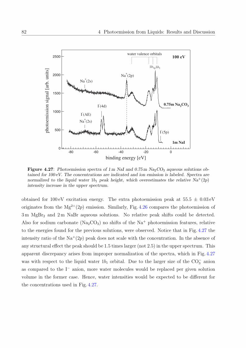
82 4 Photoemission from Liquids: Results and Discussion
2500
2000
1500
1000
500
0
phot
oem
issi
on s
igna
l [ar
b. u
nits
]
-80 -60 -40 -20 0
binding energy [eV]
0.75m Na2CO3
Na+(2p)
Na+(2s)
I-(AE)
Na+(2s)
I-(5p)
I-(4d)
1m NaI
water valence orbitals100 eV
1b1g1b1
Figure 4.27: Photoemission spectra of 1 m NaI and 0.75 m Na2CO3 aqueous solutions ob-tained for 100 eV. The concentrations are indicated and ion emission is labeled. Spectra arenormalized to the liquid water 1b1 peak height, which overestimates the relative Na+(2p)intensity increase in the upper spectrum.
obtained for 100 eV excitation energy. The extra photoemission peak at 55.5 ± 0.03 eV
originates from the Mg2+(2p) emission. Similarly, Fig. 4.26 compares the photoemission of
3 m MgBr2 and 2m NaBr aqueous solutions. No relative peak shifts could be detected.
Also for sodium carbonate (Na2CO3) no shifts of the Na+ photoemission features, relative
to the energies found for the previous solutions, were observed. Notice that in Fig. 4.27 the
intensity ratio of the Na+(2p) peak does not scale with the concentration. In the absence of
any structural effect the peak should be 1.5 times larger (not 2.5) in the upper spectrum. This
apparent discrepancy arises from improper normalization of the spectra, which in Fig. 4.27
was with respect to the liquid water 1b1 orbital. Due to the larger size of the CO−3 anion
as compared to the I− anion, more water molecules would be replaced per given solution
volume in the former case. Hence, water intensities would be expected to be different for
the concentrations used in Fig. 4.27.

4.2 Aqueous Salt Solutions 83
2500
2000
1500
1000
500
0
phot
oem
issi
on s
igna
l [ar
b. u
nits
]
-80 -60 -40 -20 0
binding energy [eV]
Na+(2p)
Na+(2s)
I-(AE)
I-(4d)
0.6m Na4[Fe(CN)6]
I-(5p)
Fe2+
1m NaI
water valence orbitals 100 eV
1b1g1b1
Figure 4.28: Photoemission spectra of 1 m NaI and 0.6m Na4[Fe(CN)6] aqueous solutionsobtained for 100 eV. The concentrations are indicated and ion emission is labeled.
Salts with complex structure. Na4[Fe(CN)6], K4[Fe(CN)6], and K3[Fe(CN)6] were
chosen as representatives of bulky and complex anions ([Fe(CN)6]4−, [Fe(CN)6]
3−) in solu-
tions. Moreover, these systems were proposed to not fully dissociate in water. The interesting
question is whether the solvated alkali cation would sense the different environment. Pho-
toemission spectra of the respective aqueous solutions (almost saturation) are presented in
Figs. 4.28 and 4.29. In Fig. 4.28 the photoemission spectra of 0.6m Na4[Fe(CN)6] and 1m
NaI aqueous solution are compared. The Na+(2p) intensities are consistent with the number
of Na atoms per water molecules, i.e. 0.0432 in latter solution, and 0.018 in the former. As
for other salts, no binding energy shift of the Na+(2p) line can be observed in the experiment.
Fig. 4.29 compares the photoemission spectrum from 0.5m K4[Fe(CN)6] solution with 1m
K3[Fe(CN)6] and 3m KI aqueous solutions. Signal from Fe2+ and Fe3+ in [Fe(CN)6]4− and
[Fe(CN)6]3− gives rise to small features at 6.2 ± 0.03 eV and 7.5 ± 0.03 eV, respectively. The
important information from both figures is that identical binding energies, within 0.03 eV,
are observed for both aqueous Na+ and K+, respectively, as indicated by the dashed vertical
lines. This result suggests that, within the limit of this experiment, identical hydration shells
exist for Na+ /K+ in NaI /KI and in Na4[Fe(CN)6] /K4[Fe(CN)6]/K3[Fe(CN)6] aqueous so-

84 4 Photoemission from Liquids: Results and Discussion
2000
1500
1000
500
0
phot
oem
issi
on s
igna
l [ar
b. u
nits
]
-40 -30 -20 -10 0
binding energy [eV]
1m K3[Fe(CN)6]
0.5m K4[Fe(CN)6]
K+(3p)
Fe3+
I-(5p)
Fe2+
3m KI
water valence orbitals 100 eV
1b1g1b1
Figure 4.29: Photoemission spectra of 3m KI, 1 m K3[Fe(CN)6] and 0.5 m K4[Fe(CN)6]aqueous solutions obtained for 100 eV. The concentrations are indicated and ion emission islabeled.
lutions. Furthermore, the absence of any extra feature in the upper spectrum suggests that
non-dissociated species either do not exist or their number is negligibly small.
In conclusion, the constant electron binding energy of aqueous iodide in different alkali-
metal salt solutions, but also in the case of a divalent ion or the more complex sodium
ferricyanide ion, is consistent with the absence of structural changes of the solvation com-
plex. The same result was inferred by different experimental methods [88, 99] as well. The
results also suggest that the solvating water molecules efficiently shield any ion-ion inter-
actions. Concerning the water binding energies, no significant effect of the interaction of
a solvating water molecule with the ion could be inferred. Thus within the limits of the
present experiment (30meV), the electronic structure is indistinguishable for solvate water
(both anion and cation solvation) and bulk water. It is worthwhile to mention that the
potential barrier between the energy well of the hydration shell and the bulk is rather low
so that it can be surmounted by the thermal energy of water molecules [87]. This together
with the continuous breaking and making of H-bonds within the H-bonding network in water
would in fact suggest only small differences of the electronic structure between hydrate and

4.2 Aqueous Salt Solutions 85
bulk water. This result matches the observation made in section 4.1.3, where it has been
shown that also the electronic structure of D2O water is not distinguishable from H2O water.
Summary of electron binding energies of aqueous cations and anions. Tables 4.8
and 4.9 summarize the measured electron binding energies and peak widths for cations and
anions, obtained for the various salt solutions discussed in this paragraph. Also contained are,
for comparison, the relevant gas-phase energies (electron binding energies of both neutrals
and the respective ions) as reported in the literature. Literature data include the first
(X0 + hν → X+ + e−) and second (X+ + hν → X2+ + e−) ionization potential (IP) of the
corresponding gas-phase alkali atom X0 (see Table 4.8). The relevant quantity for the halides
would be the first IP of the respective negative atom, Y− (Y− + hν → Y0 + e−; see Table
4.9). Finally the energy required to remove a deeper electron from the respective singly
charged atom, i.e. from X+ and Y− if available, was included. Notice that the experimental
binding energies of aqueous ions to be reported in the following result from individual Gauss-
500
400
300
200
100
0
phot
oem
issi
on s
igna
l [ar
b. u
nits
]
-80 -60 -40 -20
binding energy [eV]
I-(AE)
Na+(2p)
I-(4d)
I-(5p)
Na+(2s)
water valence orbitals
100 eV4m NaI
-40 -35 -30
binding energy [eV]
Na+(2p)
-60 -55 -50
binding energy [eV]
I-(4d)
Figure 4.30: Gauss fits to I−(4d) and Na+(2p) emission features for 4 m NaI aqueoussolution.

86 4 Photoemission from Liquids: Results and Discussion
ATOM X Eg(X0) [eV] Eg(X
+) [eV] Eaq(X+) [eV] FWHM [eV]
2s 5.39 — — —
Li 1s a 64.42 75.64 e 60.4 ± 0.07 1.4 ± 0.20
66.31
3s 5.14 — — —
2p b 37.98 47.28 e 35.4 ± 0.04 1.1 ± 0.03
Na 38.07 47.45 e
38.14
38.45
2s 71.03 80.07 e 68.0 ± 0.15 3.1 ± 0.50
4s 4.34 — — —
3p b 24.48
K 24.57 31.62 e 22.2 ± 0.06 1.4 ± 0.20
24.81 31.89 e
24.97
3s c 41.00 47.81 e — —
6s 3.89 — — —
5p 17.23 23.14 f — —
17.64
Cs d 19.06
19.12
5s 30.65 — — —
4d5/2 82.74 88.55 f 80.6 ± 0.03 1.1 ± 0.05
4d3/2 85.01 82.9 ± 0.04 1.3 ± 0.06
Table 4.8: Electron binding energies for aqueous cations obtained from the present pho-toemission study (Eaq), and the corresponding gas-phase values (Eg), as reported in theliterature. a [100], b [96], c [101], d [56], e [102], f [103]. Indicated errors are statistical errors.

4.2 Aqueous Salt Solutions 87
-80
-70
-60
-50
-40
-30
Li+(1s)
E (eV)
Li+(1s)
Na+(2p)
Na+(2s)
Na+(2p)
Na+(2s)
K+(3s)
K+(3p)
K+(3p)
Cs+(4d)
Cs+(4d)
Cs+(5p)
aq.
aq.
aq.
aq.
aq.
-70
-60
-50
-40
-30
-20
-10
Cl-(3p)
Cl-(3p)
aq. aq. aq.Br-(3d)
Br-(3d)
Br-(4p)
I-(5p)
I-(5p)
I-(5s)
I-(4d)
I-(4d)
-80
-70
-60
-50
-40
-30
Li+(1s)
Na+(2p)
Na+(2s)
Cs+(5p)
Cs+(4d)
K+(3p)
K+(3s)
Li+(1s)
Na+(2p)
Cs+(4d)
K+(3p)
Na+(2s)
gas phase liquid
-90
Figure 4.31: Comparison of electron binding energies for a given solvated cation Eaq(X+),with the respective gas-phase binding energy, Eg(X+). Binding energies of the solvatedspecies were determined in the present work (see Table 4.8). Gas-phase values were obtainedfrom the literature (see Table 4.8).
peak fitting averaged over a number of spectra. A typical fit, exemplified for Na+ and I−
features in the case of 4m aqueous NaI solution, is presented in Fig. 4.30. Binding energy
errors given in Tables 4.8 and 4.9 are statistical errors. These numbers are smaller than
the overall experimental resolution of the present experiment, which is about 200meV (see
section 3.2.1).
The experimental binding energies reported here are independent of the excitation photon
energy used (typically 60, 80, 100 eV). Furthermore, identical energies have been confirmed
irrespective of the salt concentration. Also the binding energies of the solvated ions were
found to be independent of the counter ion. For solvated alkali cations the observed energies
exhibit solvation energy shifts up to 16 eV towards lower binding energies as compared to
the gas-phase singly charged cations (column 4 vs. 3 in Table 4.8). Contrary, the halide
anion binding energies are shifted in solution towards higher energy by ca. 3 eV with respect
to the corresponding gas-phase value (column 4 vs. 3 in Table 4.9). The different behavior
of electron binding energies of gas-phase vs. aqueous species, for cations and anions, is

88 4 Photoemission from Liquids: Results and Discussion
ATOM Y Eg(Y0) [eV] Eg(Y
−) [eV] Eaq(Y−) [eV] FWHM [eV]
3p a 12.96 3.61 f 9.6 ± 0.07 0.6 ± 0.20
Cl 13.82
3s a 24.54
25.33
4p b 11.81 3.36 f 8.8 ± 0.06 0.9 ± 0.20
12.20
12.29
13.31
Br 15.27
4s c 23.77
24.06
24.24
25.86
3d5/2 — — 73.2 ± 0.07 1.2 ± 0.10
3d3/2 — — 74.3 ± 0.09 1.1 ± 0.10
5p d 10.50 3.06 f 7.7 ± 0.20 0.8 ± 0.30
11.31 8.8 ± 0.20 1.1 ± 0.30
I 12.17
14.11
5s d 20.80 15.10∗ — —
21.30
4d5/2e 57.83 57.41∗ 53.8 ± 0.03 1.0 ± 0.02
4d3/2 59.73 55.5 ± 0.03 1.0 ± 0.03
Table 4.9: Electron binding energies for halide anions in water obtained from the presentphotoemission study (Eaq), and the corresponding gas-phase values (Eg), as reported inthe literature. a [104], b [105], c [102], d [97], e [98], f [8]. The values marked with ∗ arecalculated [94]. Indicated errors are statistical errors.

4.2 Aqueous Salt Solutions 89
-70
-60
-30
-20
-10
Cl-(3p)
Cl-(3p)
aq. aq. aq.
Br-(3d)
Br-(3d)
Br-(4p)
I-(5p)
I-(5p)
I-(5s)
I-(4d)
I-(4d)
E (eV)
-70
-60
-50
-20
-10
I -(4d)
Br -(3d)
Br -(4p) I -(5p)
Cl -(3p)
Br -(4p) I -(5p)Cl -(3p)
I -(5s)
I -(4d) ?
liquidgas phase
Figure 4.32: Comparison of electron binding energy for a given solvated anion Eaq(Y −) withthe respective gas-phase binding energy Eg(Y −). Binding energies of the solvated specieswere determined in the present work (see Table 4.9). Gas-phase values were obtained fromliterature (see Table 4.9). No experimental gas-phase values reported for I−(4d).
displayed within an energy level diagram in Figs. 4.31 and 4.32, respectively (with the values
from Tables 4.8 and 4.9). In conclusion, no electron binding energy shifts, which could be
correlated with a change of the solvation shell structure, were observed as a function of the
counter ion size, charge and complexity. Since the ions considered here can be assumed to
be completely solvated by water molecules, expected energy changes should in fact be small.
One might argue that the effect is on the order of the spectral width of the ionic feature. In
other words, the observed peak width may well reflect a distribution of solvation situations,
which energetically differ by no more than the peak width. In section 6.1 it will be shown
that I−(4d) electron binding energy changes can be observed for the I−3 aqueous complex.
A comparison of the values reported here with the values predicted within a continuum
model (Born model) will be presented in section 4.2.5.

90 4 Photoemission from Liquids: Results and Discussion
4.2.3 Selected Data of Gas-Phase Alkali Halides
The following described gas-phase experiments on alkali-halide salts were motivated by var-
ious aspects. A first idea was to compare electron binding energies and Auger energies of
free molecules/atoms with the respective solvated ions. The subject is also concerned with
energy shifts of the photoemission lines as a function of the ionic character of a given bond
(molecule). The latter is known to vary with different environments of the atom (chemi-
cal shift). This aspect is, however, beyond the main line of the present work and it will
be touched upon only briefly. In addition, these gas-phase measurements also allow for a
comparison of shape resonances of a given atom/ion (iodine) in the gas phase vs. aqueous
solution.
The gas-phase spectra presented here were obtained at the U125/2-SGM beamline at
BESSY II. The alkali-halide salt was evaporated from a metal crucible heated at tempera-
tures between 400 - 600 C. Electrons were detected with a Scienta SES-2002 hemispherical
analyzer mounted at the magic angle [43] with respect to the polarization axis of the syn-
chrotron light. For monitoring the photofragments (charge-to-mass ratio) a time-of-flight
ion spectrometer was used.
Gas-phase CsX photoemission, X = F, Cl, Br, I. Similar to aqueous solutions (see
section 4.2.2), photoemission spectra of a gas-phase salt series (CsX) were measured. The
spectra from free Cs atoms and Cs halide salts obtained for 100 eV photons are displayed
in Fig. 4.33. The halogen ion derived features (at about 10 eV binding energy) are assigned
to F−(2p), Cl−(3p), Br−(4p), I−(5p) emission. Peaks correspond to the p shell spectra of
the isoelectronic rare gases, but they are noticeably broader due to the highly dissociative
nature of these ionized molecular states [106]. The strong intensity of the I−(4d) emission is
due to a shape-resonance enhancement (see section 4.2.4).
The Cs(5p) feature, in the case of atomic Cs, reveals a richer structure than the simple 2P
doublet as one would expect for p6 ionization. This results from the strong interaction in the
final state, involving the configurations 5p57s, 5p56s and 5p55d [107]. The Cs+(4d) emission
is entirely core like and therefore exhibits two features, 4d3/2 and 4d5/2. The splitting has a
constant value of 2.3 eV for all investigated species.
The only experimental data available for the free Cs+ ions is the 5p ionization energy of
23.14 eV [108]. Based on a simple model, Benson et al. [103] calculated a value of 23.13 eV
for Cs+(5p), which is in good agreement with the experimental finding. Applying the same
model for the 4d level a value of 88.55 eV was obtained.

4.2 Aqueous Salt Solutions 91
600x103
500
400
300
200
100
0
phot
oem
issi
on s
igna
l [ar
b. u
nits
]
-80 -60 -40 -20 0
binding energy [arb. units]
I-(4d)
Cs (4d)
I-(5p)
Br-(4p)
Cl-(3p)
F-(2p)
Cs (5p)Cs
(AE)
Cs+(AE)
I (AE)
Br-(3d)
Cs
CsI
CsBr
CsCl
CsF
Cs (5s)
100 eV
Figure 4.33: Photoemission spectra of Cs and Cs halides (CsF, CsCl, CsBr, CsI) in thegas phase obtained for 100 eV photon energy. These high-resolution spectra of the gas-phase molecules were obtained using a separate apparatus equipped with a Scienta electronanalyzer [56]; see text.

92 4 Photoemission from Liquids: Results and Discussion
CATION aq Cs+ Cs0 Cs+gas (CsF)gas (CsCl)gas (CsBr)gas (CsI)gas
Cs(4d5/2) 80.6 82.74 88.55 b 81.96 82.71 82.86 83.01
Cs(4d3/2) 82.9 85.01 84.31 85.01 85.16 85.28
Cs(5p) — 17.23 a 23.14 b 16.76 17.41 18.13 18.45
Table 4.10: Cs(4d) and Cs(5p) electron binding energies measured for various gas-phaseCs halides as inferred from Fig. 4.33. Cs(4d) gas-phase values are reported in the literaturea [56], b [103]. The measured value for aqueous Cs+ is also shown.
It is noted that the binding energy of the Cs(5p) and (4d) states slightly increases with
decreasing electronegativity of the halogen anion, but the values are very close to those of
the free atomic Cs0 (see Table 4.10). This might imply that in the gas phase the positive
charge of the Cs+ is being compensated by the halogen ion in such a way that the influence
on the electron binding energy is almost nonexistent. The same behavior was previously
reported for ionization of the metal cation in alkali halides molecules [103].
Gas vs. liquid photoemission spectra: Cs, (CsI)gas, (CsI)aq. Auger ener-
gies. Photoemission spectra of atomic Cs (top), gas-phase CsI (center) and aqueous solution
CsI (bottom) obtained for 100 eV photons are shown in Fig. 4.34. The energy scale is with
respect to the vacuum level; notice that all spectra align at the 1b1g water gas-phase emission
feature indicated by the dashed line. The assignment of the Cs spectrum follows the one
given in [107]; electron binding energies are in complete agreement.
The important information inferred from Fig. 4.34, as it concerns the binding energies,
is that the Cs(4d) photoemission lines from aqueous CsI shifts by ca. 2.5 eV towards lower
binding energy as compared to the gas-phase values. On the other hand, the values for
atomic Cs and gas-phase CsI are almost identical (see Fig. 4.33).
Another aspect of the gas phase-liquid comparison is the Auger emission. For both ions,
Cs+ and I−, this process was assigned to a 4d− 5p5p transition. The main observation from
Fig. 4.34 is that Auger energies are lower in the gas phase as compared to the corresponding
liquid-phase values. The effect is more pronounced for Cs, ca. 5 eV; however, the direct
comparison is hampered by the broadening of the liquid photoemission features.

4.2 Aqueous Salt Solutions 93
400x103
300
200
100
0
phot
oem
issi
on s
igna
l [ar
b. u
nits
]
-80 -60 -40 -20 0
binding energy [eV]
Cs (4d)
I-(4d)
Cs (AE)
Cs+(AE)
I (AE)
1b1g
Cs+(AE)
I-(AE)
Cs+(4d)
Cs
CsI
CsI
5ssatellite
5psatellite
gas
gas
aq
100 eV
Figure 4.34: Photoemission spectra of atomic Cs (top), gas-phase CsI (center), and aqueoussolution CsI (bottom) obtained for 100 eV photon energy. The high-resolution gas-phasespectra were obtained using a separate apparatus equipped with a Scienta electron analyzer[56]; see text.

94 4 Photoemission from Liquids: Results and Discussion
350x103
300
250
200
150
100
50
0
phot
oem
issi
on s
igna
l [ar
b. u
nits
]
-80 -60 -40 -20 0
binding energy [eV]
I-(4d)
Na+(2p)
Cs+(4d)
I-(AE)
I-(AE)
Cs+(AE)
(NaI)2
(NaI)2
Na+(2p)
I-(4d)
I-(AE)
Na+(2s)
I-(5p)
I-(5p)
5ssatellite
5psatellite
CsI
NaI
NaIaq
gas
gas
1b1g
100 eV 350x103
300
250
200
150
100
50
0
phot
oem
issi
on s
igna
l [ar
b. u
nits
]
-80 -60 -40 -20 0
binding energy [eV]
I-(4d)
Na+(2p)
Cs+(4d)
I-(AE)
I-(AE)
Cs+(AE)
(NaI)2
(NaI)2
Na+(2p)
I-(4d)
I-(AE)
Na+(2s)
I-(5p)
I-(5p)
5ssatellite
5psatellite
NaI
NaIaq
gas
1b1g
100 eV
Figure 4.35: Photoemission spectra of gas-phase CsI (top), NaI (center), and aqueoussolution NaI (bottom) obtained for 100 eV photon energy. These high-resolution gas-phasespectra were obtained using a separate apparatus equipped with a Scienta electron analyzer[56]; see text.
Gas vs. liquid photoemission spectra: (CsI)gas , (NaI)gas, (NaI)aq. Fig. 4.35 dis-
plays the photoemission spectra of gas-phase CsI, NaI, and aqueous NaI, obtained for 100 eV
photon energy. The relevant binding energies are summarized in Table 4.11. The doublet
character of the I−(4d) feature for NaI (center spectrum) results from dimer contributions;
about 25 % of the vapor is known to contain dimers [56]. An interesting result of this com-
parison is that the I−(4d) electron binding energy of aqueous I−(4d) and of the XI gas-phase
molecule is almost identical. However, probably more important is the question how these
energies relate to the I−(4d) gas-phase value. As mentioned, no reliable value has been re-
ported in the literature, which leaves open how the alkali atom affects the I−(4d) electron
binding energy. At the end of section 4.2.5, the origin of the different direction of gas-liquid
electron binding energy shifts for anions vs. cations will be discussed.

4.2 Aqueous Salt Solutions 95
ANION aq I− I0 I−gas (NaI)gas (CsI)gas
I(4d5/2) 53.8 57.83 a 57.41∗ 54.10 53.40
I(4d3/2) 55.5 59.73 a 55.84 55.10
Table 4.11: I(4d) electron binding energies measured for gas-phase CsI, NaI, and aqueousNaI as inferred from Fig. 4.35. I 0(4d) value is found in the literature a [98]. The value markedwith ∗ is calculated [94].
4.2.4 Iodide 4d Shape Resonance: Effect of Molecular Environ-
ment
It has been known for some time that the photoabsorption cross section of atoms with a closed
4d subshell, namely Xe, Cs, and Ba, are dominated by a resonance positioned above the 4d
threshold [94]. Experiments and theory show that I and I− exhibit the same behavior, i.e. a
pronounced resonance. The maximum of the resonance has been calculated to be positioned
at almost the same energy in I−, I, and I2+, near 96 eV [94]. The present experiment provides
the possibility to measure this resonance also for solvated I−.
Generally, the analysis of such resonances accounts for the competition between contin-
uum transitions 4d → εf and discrete 4d → 4f transitions [109]. A decisive part in this
competition is played by the 4f electrons, which move in an effective double-well potential
given by the sum of a Coulombic term and an angular momentum dependent term. De-
pending on the shape of the effective potential (for l ≥ 2 a potential barrier is formed),
the continuum wave function can exhibit a resonance behavior called shape resonance [110].
For low kinetic energies, the continuum function can hardly penetrate the potential bar-
rier. However, for sufficiently high kinetic energies (amounting to the height of the barrier)
the continuum function has a large amplitude in the region of the 4d orbital, which results
in a strong enhancement of the photoionization cross section. Due to the potential bar-
rier the maximum of the resonance lies several eV above the ionization threshold, resulting
in a delayed onset. For higher kinetic energies, the wave function starts to oscillate in the
atomic region, and due to resulting positive and negative portions of the radial dipole matrix
element, the cross section decreases [111].
In order to map the resonance behavior of the I−(4d), photoemission spectra of 2 m NaI
aqueous solution were measured for several photon energies, covering a range of 70 - 135 eV.
The I−(4d) photoemission intensity as a function of photon energy is displayed in Fig. 4.36

96 4 Photoemission from Liquids: Results and Discussion
5
4
3
2
1
0
rela
tive
cros
s se
ctio
n [a
rb. u
nits
]
140120100806040
photon energy [eV]
I
I+
I2
NaI (aqueous solution)
NaI (gas phase)
58.8 eV
54.8 eV
55 eV
58 eV
Figure 4.36: Partial relative cross section for aqueous I−(4d), and total relative cross sectionfor gas-phase NaI [56], I2 [112], I and I+ [95]. Arrows mark the photoionization threshold.
(top); prior to the analysis, all the spectra were normalized to the photon flux. Since the
present experimental setup did not permit measuring photoemission spectra at the magic
angle (see 4.1.3), our data had to be corrected for changes of the anisotropy parameters βi
(compare also discussion on page 59). Again, with the βi not known for the solution, one
can only use the gas phase values. For the present analysis βi values for I(4d) in molecular
CH3I were used [113]. These values turned out to be consistent with an atomic-like nature
of the I atom in the molecule; the measured anisotropy parameter of the I(4d) subshell
is presented in Fig. 4.37 [113]. In Fig. 4.36 the corrected relative cross section for aqueous
I−(4d) is displayed along with the total relative cross section for gas-phase NaI [56] and for

4.2 Aqueous Salt Solutions 97
1.5
1.0
0.5
0.0
-0.5
asym
met
ry p
aram
eter
β
30025020015010050
photon energy [eV]
Figure 4.37: Angular-distribution asymmetry parameter of the I(4d) subshell in CH3I [113].
gas-phase I2 [112], I, and I+ [95], respectively. The indicated error bars also account for the
different ionization threshold of CH3I and aqueous NaI.
Arrows mark the photoionization threshold of the respective species. The main observa-
tion from Fig. 4.36 is that the energy spacing between the 4d threshold and the resonance
maximum is rather similar for I2, I, and I+, but it gets larger for gas-phase NaI and even
larger for aqueous NaI. The resonance behavior of the wave function depends on the shape
of the 4d atomic potential; thus a change in the potential, by a different environment for
instance, might cause a change of the resonance. The data actually suggest an increase of
the potential barrier height, which would result in a larger delayed onset. It has to be em-
phasized that the present analysis of the I−(4d) shape resonance for aqueous solution may
considerably suffer from an inappropriate choice of the gas phase βi. Certainly, measuring
solution βi would be highly desirable in order to correctly interpret the data.

98 4 Photoemission from Liquids: Results and Discussion
4.2.5 Estimation of Electron Binding Energies of Aqueous Ions:
Born Solvation Model
Interpretation of photoemission data. The present experiment is concerned with re-
lating measured peak positions in a liquid photoemission experiment to electron binding
energies of the aqueous species. As in aqueous salt solutions ions are solvated, one needs to
correlate the free energy of solvation to the change of the ionization energy of the respective
ion. The situation is different as compared to photoemission from pure water, considered
in 4.1.2, where no solvation shell exists prior to the photoemission process, and furthermore
any re-orientation of the water structure (in terms of nuclear position) about the ionized
species is negligible on the time scale of the photoemission process. In the previous section
(4.2.2) it was shown that hydrated alkali cations exhibit solvation energy shifts towards lower
binding energies, while for anions the shift is towards higher binding energies. These shifts
are relative to the respective gas-phase ions, i.e. alkali X+ and halide Y−, respectively. They
are usually referred to as the liquid-phase binding-energy shift [25], which can be derived
from the Gibbs free energy of solvation, based on the Born equation [12]:
∆GBorn = − Z2e2
8πε0R(1− 1
εst) . (4.5)
As outlined above in the liquid water section (4.1.2), in this model the ion is considered as a
sphere with a point charge in its center and the solvent as a dielectric continuum with static
(relative) permittivity εst; Z, e, R and ε0 denote the charge of the ion, the unit charge, the
ion radius and the vacuum permittivity, respectively (compare also section 2.3).
Equation 4.5 generally overestimates the magnitude of the experimental solvation free
energy, which has lead to numerous modifications of the expression as has been discussed in
detail [15,24,88]. The main shortcoming of this continuum model arises from the fact that the
Born equation is valid for distances r R only. For distances r comparable to R the strength
of interaction of a water molecule with the ion exceeds that of its interaction with any other
single water molecule and consequently the preferred orientation of the water molecules
need to be accounted for [114]. A model that appears to better meet the requirements, by
accounting for the interaction with immobilized water molecules within the first hydration
shell, has been proposed by Y. Marcus [13]. This model explicitly accounts for different
interactions by not only allowing for contributions to the free energy from inside the ion
radius but also from the first hydration layer with the thickness depending on the electrostatic
field of the ion Ze/r. Specifically, the model involves (i) the cavity in which the ion is located

4.2 Aqueous Salt Solutions 99
in the water, (ii) a completely immobilized first hydration shell, and (iii) surroundings. For
the latter region the Born term is applied using the permittivity of bulk water (εst = 81.1
[16]), while ε = 1 is assumed for the first hydration shell (dielectric saturation due to strong
orientation of the water molecules). The ion radius related with region (i) can be defined
as Rion = dion−water − Rwater, where dion−water is the shortest distance between the ion and
the oxygen atoms of the water molecules in their first hydration shell (as derived from the
first minimum of the pair-correlation function gij(r)9) [88]. Rwater is an appropriate distance
that characterizes the radius of a water molecule; the average of reported values is Rwater =
0.142 nm [88]. Various simplified, rather empirical expressions for Rion have been proposed
as well, which in fact turn out to be quite useful for discussing the experimental binding
energies for aqueous ions obtained in this study. The concept followed here to calculate
∆GBorn is based on modelling the solvent molecular effects in the immediate vicinity of the
charged solute using an effective ion radius, Reff . It thus accounts, yet in a much simpler
way, also for different interactions of water very near the ion and far away. Reff was found
to be well approximated by Rcrystalion and the solvation radius Rgmax according to [15]:
Reff =Rcrystal
ion +Rgmax
2, (4.6)
where Rcrystalion is the crystal ionic radius, and Rgmax = dion−water (see above). Values for
Rcrystalion and dion−water used with equation 4.6 are presented in Table 4.12 (from Ref. [88]).
One now needs to relate the Gibbs free energy ∆GBorn, equation 4.5, to the measured
electron binding energies of solvated ions. I.e., one likes to interpret the photoemission
experiment, which involves ionization of solvated ions giving rise to a change of the ion’s
charge state (q → q ± 1), in terms of the change of the solvation free energy for the initial
and final state solvate. Then, for aqueous cations and anions, the relevant processes can be
expressed by:
X+aq + hν → X2+
aq + e−(vac), (4.7)
Y −aq + hν → Y 0
aq + e−(vac) (4.8)
Since the photoemission process is much faster than the time scale required to reorganize
the initial solvation shell, the detected photoelectron carries only the information of the orig-
inal configuration (the reorientation of the solvent molecules in terms of nuclear positions
9The distance r of the first peak in the dependence of gij(r) on r gives the shortest interatomic (inter-
nuclear) distance dij between two particles i and j.

100 4 Photoemission from Liquids: Results and Discussion
ATOM Eg(X+) Eaq(X
+) EBornaq (X+) Rcrystal
ion Rgmax Reff
X [eV] [eV] [eV] [A] [A] [A]
Li 2s — — — 0.74 c 2.08 c 1.41
1s 75.64 a 60.4 ± 0.07 60.50
3s — — —
Na 2p 47.28 a 35.4 ± 0.04 34.65 1.02 c 2.36 c 1.69
2s 80.07 a 68.0 ± 0.15 67.44
4s — — —
K 3p 31.62 a 22.2 ± 0.06 21.41 1.38 c 2.80 c 2.09
3s 47.81 a
6s — — —
5p 23.14 b — 14.32
Cs 5s 1.70 c 3.14 c 2.42
4d5/2 88.55 b 80.6 ± 0.03 79.73
4d3/2 82.9 ± 0.04
Table 4.12: Comparison between measured (Eaq) and calculated (EBornaq ) electron binding
energies using the Born continuum model. Gas-phase values are also included ( a [102],b [103]). Rcrystal
ion ( c [88]) is the crystal ionic radius, Rgmax ( c [88]) is the shortest ion-oxygenatom distance and Reff is the effective radius as defined in equation 4.6.
can be neglected due to the fast time scale [25]). In other words the energy required for
reactions 4.7 and 4.8 is the vertical ionization energy, which can be determined by photoe-
mission. The calculated electron binding energies, EBornaq , presented in the Table 4.12 were
obtained using equation 4.5 in
EBornaq = Eg + ∆G , (4.9)
with
∆G = ∆GBornf −∆GBorn
i . (4.10)
∆GBorni and ∆GBorn
f are the solvation energies for the respective initial and final state of
a given anion or cation in solution. Hence, determination of EBornaq requires to calculate
the net energy change associated with the water solvation-shell rearrangement that follows
the ionization of an ion 10. Within this simple continuum consideration, the solvation en-
10Of course, no reorientation occurs on the time scale of photoemission process. One thus calculates ∆G

4.2 Aqueous Salt Solutions 101
ATOM Eg(Y−) Eaq(Y
−) EBornaq (Y−) Rcrystal
ion Rgmax Reff
Y [eV] [eV] [eV] [A] [A] [A]
Cl 3p 3.61 a 9.6 ± 0.07 6.46 1.81 b 3.19 b 2.50
3s
4p 3.36 a 8.8 ± 0.06 6.02
Br 4s 1.96 b 3.37 b 2.67
3d5/2 73.2 ± 0.07
3d3/2 74.3 ± 0.09
5p 3.06 a 7.7 ± 0.20 5.49
8.8 ± 0.20
I 5s 15.10∗ — 17.53 2.20 b 3.65 b 2.93
4d5/2 57.41∗ 53.8 ± 0.03 59.84∗
4d3/2 55.5 ± 0.03
Table 4.13: Comparison between measured (Eaq) and calculated (EBornaq ) electron binding
energies using the Born continuum model. Gas-phase values are also included ( a [8]). Rcrystalion
( b [88]) is the crystal ionic radius, Rgmax ( b [88]) is the shortest ion-oxygen atom distanceand Reff is the effective radius as defined in equation 4.6. The asterisk for iodide indicatesthat experimental values are not available, and theoretical values were used instead [94].
ergy around a neutral atom is assumed to be negligible. A cartoon depicting the different
situations is presented in Fig. 4.38.
Since the present liquid photoemission experiment accesses vertical electron binding en-
ergies of aqueous ions (no reorientation of the water molecules on the time scale of the
photoemission process) the relevant reactions for determining ∆GBorn are equations 4.7 and
4.8. Specifically, from equation 4.10 one obtains:
∆GBorn(cation) = ∆GBorn(X2+aq )−∆GBorn(X+
aq), (4.11)
∆GBorn(anion) = ∆GBorn(Y 0aq)−∆GBorn(Y −
aq ) (4.12)
for cations and anions, respectively.
With equations 4.11 and 4.12 the observed larger binding-energy shift towards lower
for solvating the initial ion of charge q and the product ion (after photoemission) of charge (q − 1). Notice
that one may also use thermodynamically measured values (if available) of the solvation energy for cations
and anions as discussed in Ref. [24].

102 4 Photoemission from Liquids: Results and Discussion
e-
hν
Neutral water
no initial polarization about charge
t < 0 (before PE) t > 0 (time scale of PE)
ε ~ εopt
∆GfBornelectr.
EaqNeutralEgNeutral
+ 2+
e-
Hydrated cation X+aq EaqCation
∆GfBorn
∆GiBorn
EgCation
X2+
X+ already max. polarized ε is max. ~ εst
εeff = εopt+ εst
X0
X+
hν
εopt' < εeff < εst
-
e-
Hydrated anion Y-aq EaqAnion
∆GiBornY-
Y0
EgAnion
hν
already max. polarized ε is max. ~ εst
+
shift ~ - ∆GBornelectr.
shift ~ - 3∆GBorn
shift ~ ∆GBorn
E gas liquid
(more favorable in terms of H-bonding)
E
E
εopt' < εeff < εst
Figure 4.38: Schematic depicting the polarization effects for ion solvation relevant for thephotoemission process. The ovals containing arrows represent oriented and polarized watermolecules. The energy level diagrams (right side) illustrate the liquid-phase binding energyshifts in terms of the solvation free energy (∆G) relative to the respective gaseous ion. Eg
and Eaq are the electron binding energies of the gas-phase species and the hydrated species,respectively. The different direction of gas-liquid shifts for solvated anions vs. cations can bedirectly inferred from the lengths of the arrows labeled Eaq relative to Eg. The cartoons alsoindicate that shifts are larger for the case of cations.

4.2 Aqueous Salt Solutions 103
values and the smaller shift in the opposite direction for cations and anions, respectively,
can be directly explained. From equation 4.11 and equation 4.5, i.e. for the case of cations
one obtains:
∆GBorn(cation) = − 3e2
8πε0Reff
(1− 1
εst) . (4.13)
For anions, using equation 4.12 and equation 4.5 one obtains:
∆GBorn(anion) =e2
8πε0Reff
(1− 1
εst) . (4.14)
Notice that equations 4.13 and 4.14 differ by a factor of -3. Consequently, for anions the
net energy difference between the final and initial state in the liquid is on the order of
∆GBorn(anion) larger than in the gas phase, while for cations the total energy difference
between the final and initial state is smaller by about 3 ·∆GBorn(anion) as compared to the
gas phase. Hence, the anion peaks in the photoemission spectra of solution are expected to
appear at increased binding energy, whereas the cation peaks occur at lower binding energy
with the shift being larger in the latter case.
As presented in Tables 4.12 and 4.13, calculated and experimental electron binding ener-
gies, EBornaq and Eaq, respectively, agree within about 1 eV for cations. For anions the values
differ by about 2 - 6 eV. The reason for better reproducing the former values is assumed
to partly result from the fact that the total gas-liquid shift is larger in that case. Then,
any other contributions to the peak shift such as polarization screening (see 4.1.2) would
be rather negligible as they are small. This is not true for the case of anions, where this
competitiveness is of a larger concern.
It is noteworthy to mention that classical continuum dielectric models have also been
proven useful for modelling ion solvation in large (water) clusters (e.g. [115]); these systems
are of great significance to the understanding of the solvation phenomena in bulk solutions.
For I−(H2O)n clusters experimental electron binding energies were in fact shown to fit an
analogous model where the anion is solvated at the surface of the solvent cluster [116].
Photoelectron spectra of I−(H2O)n, n ≤ 60, are shown in Fig. 4.39, which was adapted from
Ref. [115]. The strong initial changes of electron binding energies up to six water molecules,
followed by reduced changes for subsequent addition of a water molecule, indicates the
formation of the first solvation shell with a coordination number of six. In 4.2.6 the relevance
of these data for the interpretation of the present results will be discussed in the context of I−
and Na+ solvation at near saturation concentration. Cluster studies of solvated alkali atoms,
e.g. Cs(H2O)n [117] and Na(H2O)n [118], indicate that for the alkali atom surrounded by

104 4 Photoemission from Liquids: Results and Discussion
1
n=0
2
3
4
5
6
7
8
9
10
15
20
25
30
40
44
49
53
60
35
binding energy [eV]6.5 5.5 4.5 3.5 2.5
Figure 4.39: Photoemissionspectra of I−(H2O)n clusters[115]. The excitation photonenergy was 7.1 eV.
more than four water molecules the ionization potential does not depend on the metal atom
but on the solvent species. In the latter work the sodium atom was proposed to spontaneously
ionize with the emitted electron getting solvated (compare 5.2.1). As opposed to the anionic
solvation these cation results are difficult to be compared with the present photoemission
data in which case electron binding energies of the solvated cation have been directly accessed
(ca. 81 and 35 eV for Cs+(4d) and Na+(2p), respectively; see Table 4.8).
In this section it has been shown that the Born continuum model can quite accurately
describe certain trends in the energetics of ion solvation. Yet, it is not an exact theory as it
does not consider any microscopic details of the solvation shell structure. It may therefore
surprise that the model works so well. There is no doubt, however, that the specific molecular
interactions between water molecules and ions of different charge and size must hold the key
to the very different solvation behavior of the different ions. Particularly this immediate

4.2 Aqueous Salt Solutions 105
(contact) interaction is barely included in the Born description, and even worse, the Born
model is strictly applicable only for distances considerably larger than the ion radius (see
section 2.3).
In the following I will touch upon some of the aspects that seem importantly related
to the microscopic solvation process. Notice that there is little input from theory yet. An
interesting question is how one can understand the different gas-liquid shifts (just discussed
above) for solvated anions vs. cations in a microscopic picture. This must have got to do
with specifically distinct interactions of a water molecule with the two types of ions. An
obvious difference is role of the H-bonding. Differences also exist for ion/atom solvation in
small water clusters as mentioned above. For cationic solvation the O-H groups will point
away from the ion (then the oxygen atom points to the ion; compare Fig. 2.5) in order to
form O-H· · ·O hydrogen bonds with bulk water molecules at the solvation shell boundary.
Notice that this is less destructive to the bulk water structure [2]. For anions, the water
molecules are bound by directional O-H· · ·Y− hydrogen bonds. For Y− = Cl−, Br−, I−,
the O-H· · ·Y− hydrogen bond is in fact observed to be weaker than the O-H· · ·O hydrogen
bond between two water molecules, and is observed to become weaker within the halogenic
series [2]. This may well have an effect on the effective dipole moment associated with
stabilizing the solvation shell. Moreover, partial charge transfer between solvent molecules
and the solute ion will be different for the two solvation situations. At present, the issue is
far from being understood, but it may be worthwhile discussing some of the observations for
gas-phase alkali halides (presented in 4.2.3) in that context. In Table 4.10 the Cs electron
binding energy (in gas-phase Csδ+Yδ−) can be seen to decrease within the halogenic series.
Even though these results await theoretical analysis in terms of charge transfer and its
dependence on the halide counter anion, it seems that alkali halide systems may be useful
to also understanding some of the electronic interactions in ion solvation by water. The
interesting result from Table 4.10 is that the measured electron binding energy for aqueous
Cs+(4d), which is ca. 82 eV, is quite similar to the Cs+(4d) energies in gas-phase CsY, being
83.5 eV (averaged over different co-ions and peak splitting). To what extend this result may,
however, answer the above question is not clear at present. As pointed out above (section
4.2.3; Table 4.11) also the I−(4d) electron binding energy is found to be very similar for
aqueous I−(4d) and for the XI gas-phase molecule, but a precise value for the I−(4d) gas-
phase energy is missing. Hence, the effect of the alkali atom on the I−(4d) binding energy
remains unclear. For the same reason it remains an open question to what extend studies
of gas-phase alkali halides may provide information to better understand ion solvation by

106 4 Photoemission from Liquids: Results and Discussion
water.
4.2.6 High-Concentration Aqueous NaI Solutions
Using 100 eV photon energy, which corresponds to the shape resonance maximum of aqueous
iodide (Fig. 4.36), it is possible to detect the I−(4d) photoemission signal for a concentration
as low as 0.1 m (e.g. in aqueous NaI). This allows the investigation of solution properties
from moderately low to saturation concentration. A particularly interesting aspect concerns
the atmospheric reactivity of aqueous sea-salt microparticles for which a relative chloride ion
surface excess was proposed by theory [119]. One then would like to better understand the
interaction between solvate complexes. It seems feasible that for sufficiently high density
of solvate complexes the latter may attract each other, and, for a given case, the simple
solvation shell might be no longer energetically favorable. In fact, the assumption of perfectly
separated ions by the polar solvent molecules (Debye-Huckel model for electrolytes [90])
has been known to fail for high salt concentrations [119, 120]. Several mechanisms have
been suggested, including ion association (ion pairing) with various forms of solvation shell
sharing [87,121]. Clearly, investigating such processes by the surface-sensitive photoemission
may provide useful information on structural details of the solvation complexes.
Near saturation limit. Figs. 4.40 and 4.41 display photoemission spectra of aqueous
NaI solutions for the low and the high salt concentration range, respectively, obtained for
100 eV photons. Fig. 4.40 covers the 0.1 to 1.0m range, and Fig.4.41 shows spectra for 0.5 to
12.0 m NaI concentration. The highest concentration investigated here corresponds to nearly
saturation. With a solubility of 184 g/cm3, saturation occurs at about 13m concentration.
Since experimental handling of such high concentrations in terms of crystallization rate and
potential changes (compare section 4.3) is difficult, the highest concentration investigated
here was 12.0m. The spectra in Figs. 4.40 and 4.41 are vertically displaced relative to each
other, and normalized with respect to the synchrotron flux. The spectral assignments was
adapted from the preceding paragraphs. Great care was taken to maintain constant experi-
mental conditions for obtaining all spectra in each figure, as this is important for accessing
absolute signal attenuation/increase for varying salt concentration. In order to follow the
emission intensities of both ions as a function of concentration, the corresponding peak in-
tegrals (based on Gaussian peak fitting) of the I−(4d) and the Na+(2p) features have been
evaluated. The result is presented in Fig. 4.42. The main figure shows the photoemission in-
tensities for both anions and cations over the full concentration range, and the inset presents

4.2 Aqueous Salt Solutions 107
3000
2000
1000
0
phot
oem
issi
on s
igna
l [ar
b. u
nits
]
-100 -80 -60 -40 -20 0
binding energy [eV]
I-(4d)
I-(AE)
Na+(2p)
I-(5p)
Na+(2s)
0.1m NaI
0.2m NaI
0.4m NaI
0.6m NaI
1.0m NaI
water valence orbitals100 eV
1b1g1b1
Figure 4.40: Photoemission spectra of NaI aqueous solution obtained for different saltconcentrations as labeled. Intensities were normalized to the synchrotron photon flux. Theexcitation photon energy was 100 eV.
data for the lower concentrations only. Obviously, the data show no evidence for any dif-
ferential surface effect for anions vs. cations; intensities for both ions behave identically.
Hence, no anion surface excess can be inferred from the data (see below). However, the
present study clearly shows that for concentrations larger than 2m NaI the ion signals in-
crease no longer linearly (Fig. 4.42). In order to also quantify the water signal attenuation
in Fig. 4.43 the dependence of the water photoemission intensity as a function of the salt
concentration is presented. The decrease of the water signal can be qualitatively explained
by water molecules being replaced by salt ions.
From the ion signal plot as a function of the concentration (Fig. 4.42), and being aware of
the surface sensitivity of the present photoemission study, one concludes that for sufficiently
large salt concentration, ion densities must be lower at the surface than in the bulk solution.
Such a depletion may simply reflect that for near-saturation a larger number of ions can be
stabilized by solvation shells in the bulk, as compared to the surface. High concentrations
of ions may only exist in the bulk as all inter-complex dipoles average out, while unbalanced
dipoles in the case of a surface are energetically unfavorable. Compare also the discussion of

108 4 Photoemission from Liquids: Results and Discussion
8000
6000
4000
2000
0
phot
oem
issi
on s
igna
l [ar
b. u
nits
]
-80 -60 -40 -20 0
binding energy [eV]
Na+(2p)
Na+(2s)
I-(AE)
I-(4d)
I-(5p)
0.5m NaI1m NaI2m NaI4m NaI6m NaI8m NaI
10m NaI12m NaI
water valence orbitals
water
100 eV
1b1g 1b1
700
500
300
100-70 -60 -50 -40 -30
12m NaI
0.5m NaI
I-(4d)
Na+(2p)
Figure 4.41: Photoemission spectra of NaI aqueous solution obtained for different saltconcentrations as labeled. Intensities were normalized to the synchrotron photon flux. Theexcitation photon energy was 100 eV. The inset displays the spectra of lowest and highestsalt concentration on top of each other, but scaled to have identical intensities. From thiscomparison constant electron binding energies of both I−(4d) and Na+(2p) as a function ofsalt concentration are inferred.
the iodide signal for the surface-active tetrabutylammoniumiodide (But4NI) in section 4.3.
Peak positions of both Na+ and I− features are found to be constant for all concentrations
studied. This has been indicated in the inset of Fig. 4.41 for 0.5 and 12m NaI concentration.
Fig. 4.44 displays I−(4d) electron binding energies, as obtained by careful Gaussian peak
fitting (compare Fig. 4.30), as a function of the NaI concentration. Statistical errors are
indicated; systematic errors are not accounted for. From Fig. 4.44 it is concluded that
binding energy shifts are no larger than ca. 30 meV, and also no obvious trend as to the
direction of a peak shift can be inferred. The fact that the electron binding energy not even
changes for near-saturation concentration may surprise. In section 4.3.1 two principle sources
for peak shifts will be discussed in detail. One results from the decreasing coordination

4.2 Aqueous Salt Solutions 109
I-(4d)
Na+(2p)
concentration [NaI/H2O]3.6 7.2 10.8 14.4 18.8 21.6 x10⁻²
1.00.80.60.40.20.0ar
ea [
arb.
uni
ts]
concentration [mol/kg]
4000
3000
2000
1000
0
area
[ar
b. u
nits
]
121086420
concentration [mol/kg]
Figure 4.42: Increase of the I−(4d) and Na+(2p) photoemission signal as a function of theNaI concentration (based on peak fitting and integration of spectra in Figs. 4.40 and 4.41).The inset presents data for low concentrations. The sub-linear increase for concentrationslarger than 2 m is attributed to surface depletion of bulk ions, i.e. relatively lower ion densityas compared to the bulk solution.
(solvation) number (smaller shell as there are fewer water molecules available), and the
other is associated with surface dipoles due to an electric double layer. The latter effect
would cause the I−/Na+ ion intensity ratio to change, which is not the case here. Hence, the
present results are in disagreement with previous theoretical results [89] according to which
the large anion, favors an asymmetric location in the solvation cage (which would give rise
to an anion surface excess).
It is interesting to note that for the 12m concentration, the ratio of water molecules
to salt molecules (about 5:1) implies that the solvation structure must be different than in
the Debye-Huckel limit, where each ion is individually solvated. This raises the question
whether or not this experiment is sensitive to solvation structural changes (e.g. ion pairing
and the related propensity for surface anion excess). It certainly should be, unless the
effect is compensated by other contributions. At this point a comparison with respective
cluster studies would seem interesting as these systems may be considered valuable models

110 4 Photoemission from Liquids: Results and Discussion
1.0
0.9
0.8
0.7
0.6
0.5
area
1b 1
[arb
. uni
ts]
121086420
concentration [mol/kg]
water signal attenuation
Figure 4.43: Decrease of the 1b1 liquid water photoemission signal as a function of NaIconcentration.
providing microscopic details of the ion-solvent and solvent-solvent interaction. Studies of
larger clusters, here we are concerned with halide anions solvated in water clusters, containing
tens of solvent molecules or even more, may elucidate the evolution of solvation layers in
confined environments, and their convergence to bulk properties [115] (compare to section
4.2.5). The particular interest here is in the experimental electron binding energy obtained
for I−(H2O)n and the related dependence on n. It has to be pointed out, however, that for
clusters surface solvation has been proposed to be energetically favorable (see page 103).
Notice that the comparison with cluster studies may provide information on the distance
over which the water feels the ion. 11
As opposed to clusters, in macroscopic systems surface solvation might be prevented. If
surface anions, solvated by incomplete shells, would exist one would have expected to at least
observe a change of the electron binding energy. In fact the absence of surface solvation for
bulk NaI aqueous solution would be consistent with the existence of the depletion layer in
which full-shell solvation is maintained by keeping ions away from the very liquid/vacuum
11The situation may be more complicated as in the cluster studies particularly ion-ion interactions are
absent.

4.2 Aqueous Salt Solutions 111
-54.22
-54.20
-54.18
-54.16
-54.14
-54.12
-54.10I- (4
d) p
ositi
on [
eV]
121086420
concentration [mol/kg]
I-(4d5/2) position
Figure 4.44: Experimental I−(4d5/2) electron binding energies as a function of the NaI con-centration. Data result from fitting the spectra shown in Fig. 4.41. No statistically significantbinding energy shifts can be inferred.
boundary. It is interesting to note that cluster studies yield identical electron binding energies
(7.7 eV) for n ' 100 (extrapolated from Ref. [115], see Fig. 4.39) as obtained for the bulk
solution. Whether this information is useful for the interpretation of the present data is
difficult to judge. It should be pointed out that fundamental differences exist between liquid
phase and cluster solvation. In the latter case three extra solvation contributions have to
be considered: (i) the formation of a spherical cavity in the solvent continuum, (ii) the
introduction into this cavity of an ion-solvent molecule cluster performed in vacuum, and
(iii) the rearrangement of the solvent molecule in the vicinity of the cluster [10].

112 4 Photoemission from Liquids: Results and Discussion
4.3 Surface Segregation
A special property of hydrogen bonding (H-bonding) in water is the hydrophobicity which
causes non-polar molecules such as hydrocarbon chains to associate with each other in an
aqueous environment. Here, water ’squeezes’ non-polar molecules together, and as a con-
sequence the dissociated hydrophobic ions will be non-uniformly distributed in the solvent.
Often, considerable surface accumulation occurs, which is referred to as surface activity.
The focus of this section is on the surface-active tetrabutylammoniumiodide (C4H9)4NI
(But4NI) dissolved in water. The But4N+ cation is one of the most efficient and intensively
investigated phase-transfer catalysts 12 [122] by numerous methods. But4NI in formamide
is known to form a surface layer of about 1 nm thickness which roughly corresponds to the
diameter of the But4N+ ion [123,124].
Given the high surface sensitivity of photoemission, the method would seem predestinated
to investigate the nature of such a surface-active system. Specifically, one should be able to
identify surface iodide and particularly the existence of an electric double layer (see below)
by spectral changes of the photoemission spectra. This would include both peak shifts
and relative signal variations. Detailed analysis of the spectra might even allow to infer
information on the microscopic structure of the segregation layer. The only photoemission
study of But4N+I− aqueous solution was performed by Watanabe [125]. He used a rotating
target and monochromatized light from a hydrogen lamp, the experiment was, however,
limited to photoionization threshold (see also section 4.2). But4N+I− dissociates in water
and the large hydrophobic But4N+ cations segregate at the surface. For electrostatic reasons
surface But4N+ ions are always accompanied by their counter ion, iodide [123, 124]. The
surface activity of the But4NI was shown to correlate with a decrease of surface tension, as
this minimizes the energy of the system [126]. Angle-resolved X-ray spectroscopy (ARXPS)
revealed no relative ion surface excess, i.e. no differential segregation between the cations
But4N+ and anions I− within the depth resolution of few A [127]. The existence of iodide
in the topmost layer, giving rise to an electric double layer, was confirmed by metastable
induced electron spectroscopy (MIES) [128]. These previous spectroscopic techniques were
12Phase transfer catalysis is a concept that relates to chemical reactions where the reactants are in two
separate phases. In such cases, the rates and yields are very often limited by the slow transport of reactants
from one phase to another. Phase transfer catalysts were found to be useful in transporting the reactants,
thus increasing yields and rates, and facilitating reactions which are otherwise not feasible or very difficult
to carry out.

4.3 Surface Segregation 113
exclusively performed for organic solvents, often formamide, as such an organic solvent can
be easier handled under high-vacuum conditions. Hydrophobic effects are expected, however,
to be more pronounced for water.
Other investigations of But4N+I− dissolved in water, e.g. measurements of osmotic and
activity coefficients, have shown that the surface activity increases for increasing alkyl chain
length [126]. Furthermore, But4NI surface segregation strongly depends on the counter ion;
it decreases in the order I− > Br− > Cl− [126]. This behavior was explained in terms of
the so called solvent structure-enforced ion pairing [123, 129]. The model assumes that the
total disturbance of the water structure, by both the anions and the cations, is minimized if,
e.g. But4N+ and I− are put in the same cavity of the disturbed water structure. Then, for a
smaller radius, i.e. for a better dissolvable ion, the tendency for ion pairing is reduced. Notice
that this pairing mechanism would also allow for a higher surface concentration as compared
to the case of unpaired ions due to the more compact solvate complex structure [123].
Here, photoemission spectra from But4NI aqueous solution as a function of the salt
concentration are reported. Particular focus is on the identification of the completed seg-
regated surface layer by following the relative intensity changes of the photoemission signal
of the iodide anion as a function of the salt concentration. Furthermore, another question
is whether changes of the hydration shell structure (solvent coordination), particularly for
surface vs. deeper ions, may be identified by different electron binding energies. Finally,
results on the exchange of iodide located within the segregation layer with bulk solution
bromide are presented. The experiments were performed in order to elaborate on the effect
of the anion size, specifically on the reluctance of the large I− anion to exchange with the
smaller Br− anion. Photoemission spectra are presented for But4NI dissolved in aqueous
XBr solutions, X = Na, K, Cs. The effect of the counter cation will be addressed as well.

114 4 Photoemission from Liquids: Results and Discussion
4.3.1 Identification of the Completed Tetrabutylammoniumiodide
(But4NI) Monolayer on the Water Surface
Photoemission spectra of pure water, 2m NaI, and 0.025m But4NI aqueous solutions ob-
tained for 100 eV photon energy are displayed in Fig. 4.45. The spectra are vertically dis-
placed with respect to each other, and relative intensities are properly matched. Scaling was
5000
4000
3000
2000
1000
0
phot
oem
issi
on s
igna
l [ar
b. u
nits
]
-80 -60 -40 -20 0
binding energy [eV]
1b1g 1b1
100 eV I-(4d)
+
Na+(2p)
I-(AE)
I-(5p)
I-(5p)
I-(AE)
Na+(2s)
2m NaI
0.025m But4NI
water valence orbitals
But4N
water
Figure 4.45: Photoemission spectra of pure water, 1 m NaI, and 0.02 m But4NI aqueoussolutions, respectively. For normalization procedure see text. I−(4d) intensities are almostidentical even though the concentrations differ by a factor of 80. This is a direct evidence forBut4NI surface segregation.
done with reference to Fig. 4.46 (see below) in order to account for the relative photoemis-
sion signal attenuation of the water 1b1 (liquid) emission by the overlayer. The energy axis
refers to electron binding energies with respect to 1b1g, as described above (section 4.1.1).
In the photoemission spectra from aqueous But4NI and NaI solutions (top and center spec-
tra in Fig. 4.45) one can recognize the underlying H2O molecular orbital features, 2a1, 1b2,
3a1, 1b1 (see 4.1.1). The features from the Na+ and I− emission are labeled according to
the previous spectra. Although the concentrations are completely different, the I−(4d) peak
is found to be of almost identical intensity for both solution spectra. This directly points
to substantial But4N+I− surface segregation, assuming that anions and cations segregate

4.3 Surface Segregation 115
pair-wise (see below). With the I−(4d) iodide signal ratio I−(But4NI)/I−(NaI) being 0.9, as
inferred from Fig. 4.45, and an iodide concentration ratio of 1/80, one obtains an effective
segregation factor of about 70 for the given concentrations. It is useful to now estimate the
fraction of iodide ions residing at the surface vs. the number of ions inside the bulk solution
volume as this would be a more meaningful quantity (relative segregation). For a given salt
(But4NI) concentration this fraction may be obtained by comparing the total volume of ions
in the solution, and the volume available at the surface. Certainly the result depends on the
particular geometry. For 0.02m But4NI solution, one obtains a relative surface segregation
factor of > 100. 13
Further information on surface structural details may be obtained from the evolution
of the photoemission signal as a function of the But4NI concentration. Selected spectra of
different concentrations, 0.005, 0.015, 0.025, 0.030, 0.040m But4NI in water are displayed in
Fig. 4.46 together with a reference water spectrum. The intensities in the figure are normal-
ized with respect to the ring current, hence relative intensity changes directly correlate with
true relative variations of the emission signal. For the purpose of displaying the evolution of
emission intensities, the But4NI solution spectra in Fig. 4.46 have all been energy-shifted in
order to align at the liquid water 1b1 feature (at 11.16 eV binding energy, see section 4.1.2).
The amount and the origin of these differential peak shifts will be addressed below. The
main result from Fig. 4.46 is that the I−(4d) signal steadily increases up to about 0.02m
But4NI concentration, which corresponds to 33.3% of maximum solubility, and levels off
for larger concentrations. The water signal, on the other hand, is attenuated as the over-
layer grows. For a more quantitative analysis the iodide signal increase as a function of the
But4NI concentration is displayed in Fig. 4.47a. Each data point represents the integral of
the I−(4d) emission feature assuming Gaussians on a constant background. Indicated errors
are statistical errors. Two regimes of different slopes may be clearly identified, and the
break near 0.02m But4NI concentration might be attributed to the completion of the salt
monolayer on top of the water surface. A similar behavior is known for adsorbate systems, if
growth proceeds layer-by-layer as, for instance, C60/Ni [130]. This is the first time that the
layer completion on a solution surface was probed by photoemission. In adsorbate/crystal
13Consider an outer shell volume Vsurf of the liquid (thickness 1 nm, which is the diameter of But4N+
cation). With r the jet radius, l the jet length, and R the ion radius, Vsurf = 4πRl(r−R). The total volume
of the jet is Vjet = πr2l and thus the ratio Vjet/Vsurf = 4R/r. For R = 5 A and r = 3 µm, one obtains a
ratio of volume sites vs. surface sites of 1.5 × 10³. For 0.02 m But4NI concentration, the effective number
ratio of volume vs. surface ions is ca. 10, which is an enormous effect yielding a segregation factor > 100.

116 4 Photoemission from Liquids: Results and Discussion
I-(4d)
I-(AE)
I-(5p)
TBAI+
5000
4000
3000
2000
1000
0
phot
oem
issi
on s
igna
l [ar
b. u
nits
]
-80 -60 -40 -20 0
binding energy [eV]
I-(4d)
I-(5p)
But4N+I
-(AE)
0.005m
0.015m
0.025m
0.030m
0.040m
water valence orbitals
water
1b1g1b1
100 eV
Figure 4.46: Photoemission spectra of But4NI aqueous solution obtained for different saltconcentrations, as labeled. Intensities are normalized to the synchrotron photon flux. Theexcitation photon energy was 100 eV. For the purpose of comparing relative intensities smallspectral shifts have been compensated for (see text).
systems one typically observes several linear, equally spaced segments in the uptake, where
each break correlates with the completion of a different layer. Only one break is observed
in the present experiment since only one single monolayer can be formed by the surfactant.
This, in a simple picture, reflects the low salt solubility and the fact that once the layer is
saturated no additional But4N+ can be stabilized at the surface. Moreover, the mere exis-
tence of a break in the uptake in Fig. 4.47a confirms that the salt concentration must change
significantly just below the overlayer. The almost constant signal for concentrations above
0.02m But4NI is another corroboration of rather insignificant ion enrichment (second layer)
next to the dipole layer. In fact, any slight signal increase may be identified with the filling
of the still remaining surface sites.
Identifying 0.02m concentration with the surface monolayer coverage in the present jet
experiment would imply that at the point where the synchrotron light intersects the jet
(1mm after the nozzle, which corresponds to 10−5 s travel time) a sufficiently large number
of bulk solution molecules had diffused to the surface. From Fick’s law of diffusion the mean

4.3 Surface Segregation 117
1.0
0.9
0.8
0.7
0.6
area
2a 1
[arb
. uni
ts]
0.040.030.020.010
concentration [mol/kg]
water signal attenuation
1600
1400
1200
1000
800
600
400
200
0
area
I- (4
d) [
arb.
uni
ts]
0.040.030.020.010
concentration [mol/kg]
25
20
15
10
area
2a 1
[arb
. uni
ts]
40x10-3
3020100
concentration [mol/kg]
concentration [But4NI/H2O]
400
300
200
100
0
area
I- (4
d) [
arb.
uni
ts]
40x10-3
3020100
concentration [mol/kg]
0 2 4 6 8 x10⁻⁴
N+
CH3
CH3
H3C
H3C I-
N But
But
But
But+
I-
area I-(4d)
8 x10⁻⁴
6420
-
1600
1200
800
400
0
area
I(4
d) [
arb.
uni
ts]
0.040.030.020.010concentration [mol/kg]
a)
b)
Figure 4.47: (Top) Increase of the I−(4d) photoemission signal as a function of the But4NIconcentration (based on peak fitting and integration of spectra in Fig. 4.46). The straight line(no fit) at lower concentrations suggests the successive completion of the surface segregationlayer. The break off near 0.02 m concentration characterizes the onset of electron emissionthrough the completed segregation layer. The inset presents a fit to the data using (1−e−ax)where a is a fit parameter. Notice that the fit poorly reproduces the signal intensities inthe saturation regime as it does not account for the varying information depth. (Bottom)Analogue analysis and plot for the liquid-water signal (2a1) decrease.

118 4 Photoemission from Liquids: Results and Discussion
distance L over which an ion travels through a liquid medium can be expressed as [46]:
L =√
4Dt , (4.15)
where D is the diffusion constant and t is the time. For D = 0.52×10⁻⁵ cm2/s and t = 10−5 s
one obtains a diffusion length of ca. 140 nm, which corresponds to about 450 monolayers of
water. Hence, only molecules within a 140 nm thick outer shell are able to diffuse to the
surface. Clearly, diffusion from deeper locations would be possible if the experiment was
performed at a distance farther than 1mm downstream from the nozzle. For the present
experimental conditions one can estimate that indeed at a concentration of about 0.02m
But4NI sufficient salt molecules exist in the outer layer of the jet. Hence, the travelling
time of the jet and the diffusion constant just match in a way to allow for the formation
of a full But4NI surface monolayer. 14 One may consider this result to also support the
interpretation of the data in Fig. 4.47a in terms of linear segments, but still, this is not fully
conclusive. For that reason the inset in Fig. 4.47a presents a fit, which models the formation
of the segregation layer up to saturation. Here the build up is assumed to be proportional
to (1− e−ax), where a is a fit parameter representing the concentration with respect to the
saturation concentration. Even though the experimental data can be fit reasonably well, the
simple model cannot account for any effect of the photoelectron information depth, which
inherently leads to relative signal attenuation. In fact the linear segments fit the data better,
particularly in the saturation regime.
Qualitatively similar information can be inferred by analyzing the attenuation of the
water signal for increasing But4NI coverage. The corresponding plot is presented in Fig. 4.47b
for the 2a1 water orbital. As before, data points represent integrals based on Gaussian peak
fitting on a constant background. Also the water attenuation behavior can be interpreted
to reflect the completion of the segregation surface layer near 0.02m concentration. This is
suggested by the straight lines (no fit). Notice that the values in the case of water are not
as accurate as for the iodide signal presented in the top figure. Clearly the latter signal is
the more reliable probe in the present experiments due to the intense I−(4d) doublet peak
on a smooth background.
14Consider an outer shell volume V of the liquid jet (thickness 140 nm) which contains N = cNAV
molecules. The volume of these N molecules is Vmolec = 4πR3
3 N . Equating Vmolec with the surface vol-
ume (volume of one surface monolayer), Vsurf = 4πRl(r − R), one calculates the concentration being
c = 3r/πNAR2L(2r − L). With the Avogadro number NA = 6.02 × 10²³mol−1, the ion radius R = 0.5 nm,
the jet radius r = 3 µm, and the diffusion length L = 140 nm one obtains a concentration of 0.023 mol/kg.

4.3 Surface Segregation 119
The water signal attenuation is related to the solute layer thickness d and the electron
mean free path λe by the following expression [40]:
Iad = I0 exp(−d
λe
) . (4.16)
Here I0 and Iad denote the photoemission intensity of the uncovered (pure) water and the
salt-covered water, respectively. Hence, assuming λe = 3 - 4 nm for 90 eV electrons 15 (see
Fig. 3.4) equation 4.16 may be used to cross-check the segregation layer thickness. According
to Fig. 4.47b, at 0.02m But4NI concentration, the water signal is being reduced by about
32% with respect to its intensity for pure water. Then equation 4.16 yields d = 1.2 nm which
is close to the expected value of 1.0 nm [123].
Regarding the iodide intensities it is interesting to compare the data for NaI (Fig. 4.42)
and for But4NI (Fig. 4.47) aqueous solutions. Since the concentrations used for these two
situations were very different, Fig. 4.48 presents the I−(4d) intensities for both experiments
vs. the logarithm of the concentration. Relative intensities were inferred from the previous
spectra, and the I−(4d) intensity for the saturated But4NI solution has been set to unity. For
the highest NaI concentration, 12m, the iodide signal is about a factor of 4 larger than for the
But4NI solution at saturation coverage, which at a first glance may be a surprise. The main
reason for this intensity ratio is the size of the corresponding ions. As depicted in the simple
cartoon in Fig. 4.48, at the surface, assuming close packing and neglecting solvation shells,
the ratio of But4NI surface sites vs. NaI surface sites is about 1 : 2.3. This corresponds to the
ratio of the respective ion radii, 5 A vs. 2.2 A [10, 88]. Radii in the cartoons (Fig. 4.48) are
drawn to scale. Notice that the point at which the I−(4d) signal from NaI solution gets near
2.5 times the intensity of I−(4d) from saturated But4NI just corresponds to the concentration
at which the I−(4d) begins deviating from the linear increase (Fig. 4.48). This might well
corroborate the earlier interpretation of maximum accommodation of solvated ions near the
surface. The signal increase beyond a factor of 2.5 must be attributed to the emission
contributions from deeper layers. As depicted in the cartoons of Fig. 4.48 contributions from
deeper layers in the But4NI case are negligible because of the low concentration of But4N+
and I− ions everywhere in the bulk. Notice that the electron mean free path is, however,
larger than the segregation layer thickness. Hence, in the case of NaI solution, where the ions
are homogeneously dispersed throughout the bulk solution, I−(4d) photoelectrons can also
15Notice that this time (compare page 60 for water) the thickness of one monolayer corresponds to ca. 1
nm, which is the size of the But4N+ ion. In Ref. [123] λe was found to be ca. 2.5 nm, which is somewhat
smaller than the value assumed here.

120 4 Photoemission from Liquids: Results and Discussion
Figure 4.48: Comparison of the relative I−(4d) emission intensity obtained for But4NI andNaI aqueous solutions as a function of the respective salt concentrations. The concentration ispresented on a logarithmic scale since very different concentrations are required to obtain ei-ther identical photoemission signal intensity or saturation concentration (compare Figs. 4.42and 4.47). Notice, that about the 80 times higher NaI salt concentration corresponds tothe But4NI maximum signal (for saturation coverage). The cartoons illustrate the differentstructural character of the near surface region of the two solutions. For But4NI, near satura-tion, the large anion-cation ’pairs’ form the segregation layer while the bulk concentration iscomparably low. I.e., within the range of detection, the maximum electron mean free pathλe (as indicated), signal contribution from any deeper layers is negligible. In contrary, forNaI solutions the ions are almost homogeneously dispersed, and photoemission signal fromdeeper layers will considerably contribute to the total signal, which is about 4 times larger(for saturation) as compared to But4NI. Large, medium and small circles represent But4N
+,I− and Na+ ions. The ion radii are 5 A, 2.2 A and 1 A for But4N
+, I− and Na+, respectively.In this simple cartoon no solvation shells were taken into account.
contribute from larger distances. In fact assuming a layer thickness d = 4.4 A (which is the
I− diameter), and using equation 4.16 one calculates that the measured total I−(4d) signal is
effectively generated by photoelectrons originating from within the first 3 - 4 layers. 16 This
16From Fig. 4.48 maximum signal for the But4N+ monolayer is 1. For the I− ion being two times smaller,
the corresponding signal would be I0 = 2. Accounting for contributions originating from deeper layers, the

4.3 Surface Segregation 121
5000
4000
3000
2000
1000
0
phot
oem
issi
on s
igna
l [ar
b. u
nits
]
-100 -80 -60 -40 -20 0
binding energy [eV]
I-(AE)
I-(4d)
But4N+
I-(5p)
water
0.005m
0.015m
0.030m
water valence orbitals100 eV
1b1g1b1
Figure 4.49: Full-range photoemission spectra, including the cutoff region, from aqueousBut4NI obtained for different concentrations (selection from Fig. 4.46). Spectra are displayedas measured, i.e. the indicated peak shifts correspond to true apparent binding energy dif-ferences (see text). Notice that all spectra are characterized by the identical cutoff (compareFig. 4.50). The initial shift of the liquid main features to nominally higher binding energies(for the lowest concentration) is considered an experimental artifact. The successive energyshifts to lower binding energy for higher concentrations is largely assigned to a change of thesolution work function due to an increasing molecular surface dipole density.
is a reasonable value for 50 eV electrons (see Fig. 3.4).
The other important result obtained from the segregated But4NI is the spectral energy
shift shown in Fig. 4.49. The figure displays a selection of photoemission spectra (from
Fig. 4.46) as measured, i.e. without any energy offset, but including the low kinetic energy
cutoff region. One observes that all distinct liquid features of a given spectrum are uniformly
shifted for different concentrations as indicated by vertical lines. The 1b1g water gas-phase
peak also shifts, however, by a smaller amount. Rigid shifts can be attributed to work
function changes, ∆Φdipole, associated with the molecular surface dipoles within the electric
double layer. In the present experiment, however, additional effects have to be accounted
maximum signal can be expressed by the following sum: I = I0 + I0exp(− 2dλ ) + I0exp(− 3d
λ ). Then, for d =
4.4 A and a mean free path λ ' 30 A, one obtains I = 4.7, which is somewhat larger than the actual value
of 3.8 in Fig. 4.48.

122 4 Photoemission from Liquids: Results and Discussion
Concentration Measured peak positions [eV]
[mol/kg] 1b1 (liq) I−(4d) I−(5p) [125] I−(4d) - 1b1 (liq)
0 11.28(4) — — —
0.005 11.67(5) 54.25(3) 6.60 42.58(8)
0.015 11.06(5) 53.72(3) 6.30 42.66(8)
0.025 10.88(4) 53.41(3) 6.20 42.53(7)
0.030 10.83(4) 53.37(3) 6.24 42.54(7)
0.040 10.78(4) 53.28(3) 6.20 42.53(7)
Table 4.14: Experimental peak positions (apparent electron binding energies), with respectto the water 1b1g orbital (12.6 eV), for But4NI aqueous solutions as a function of the saltconcentration. The right column is the energy difference between the I−(4d) and the 1b1
(liquid) peak position. This value is almost constant, which rules out any true electronbinding energy shifts (for instance due to relative dehydration).
for since liquid and gas-phase features shifts are not identical. These extra potentials are
artifacts caused by salt adsorption on the surface of the analyzer skimmer. Distinguishing the
effect quantitatively from the actual surface potential shift is difficult and further experiments
need to be performed. Here this artifact will not be considered in further detail. Notice that
also the large energy shift towards nominally higher binding energies with respect to the
liquid water features, for the lowest But4NI concentration, is considered an artifact. A rough
estimation of the surface dipole contribution to the shift may be obtained by considering the
peak shifts with respect to the water 1b1g gas-phase binding energy. In paragraph 4.1.1 this
energy was shown to be a well-defined external reference, which may be not necessarily true
in the presence of extra potentials. Table 4.14 presents apparent binding energy shifts of the
water 1b1 (liquid), I−(4d), and I−(5p) [125] orbitals inferred by fixing the respective water
1b1g gas-phase feature at 12.6 eV. The table also includes the energy spacing between I−(4d)
and 1b1 (liquid) peaks. The fact that this spacing (or any other between liquid features) is
independent of the concentration implies that no differential binding energy changes occur
for the liquid features. This conclusion contradicts a previous report [125], which attributes
the observed spectral shifts to dehydration effects of surface iodide, but entirely neglects
surface dipole effects. Obviously this discrepancy arises from the fact that the study in
Ref. [125] reports mere threshold energies, and is lacking a well-defined reference energy,
evidently leading to a misinterpretation of the data.
This aspect will be considered in further detail by discussing the spectral cutoff, which

4.3 Surface Segregation 123
pure water 'segregated' surface dipole
Ekin
Φ (IP)
hν
Evac
Φ' (IP')
∆Φdipole
BE
BEEF (HOMO)
E'kin=Ekin + ∆Φdipole
+-
+-
a)
b)
spectral shift
msurface
∆E
Figure 4.50: a) Schematic energy level diagram illustrating the origin of the observed (rigid)spectral energy shifts for the But4NI solution. In the absence of surface dipoles (pure water;Fig. 4.44 left) the measured electron kinetic energy, Ekin, is given by Ekin = hν − BE − Φ,where hν is the excitation photon energy, BE is the electron binding energy, and Φ denotesthe work function. The presence of surface dipoles (direction as shown in Fig. 4.44b; right)causes a decrease of the work function, ∆Φdipole, which for level alignment with respect tothe vacuum level, leads to a larger maximum kinetic energy measured in the photoemissionspectra. This is accompanied by a larger width of the entire spectrum (as experimentallyobserved; see Fig. 4.49). Full and open circles denote electrons and holes, respectively. b)Cartoon of the location and the orientation of the But4N
+I− molecular surface dipole.
is inherently related to the sample work function. Apparently, for the liquid jet the orbital
energies are pinned to the vacuum level. (Only) in this case a change of the liquid-sample
work function would result in an increase/decrease of the measured maximum kinetic energy
of the photoelectrons, which is accompanied by a decrease/increase of the width of the
photoemission spectrum by ∆E = hν − ∆Φdipole. Notice that for alignment at the Fermi

124 4 Photoemission from Liquids: Results and Discussion
54.2
54.0
53.8
53.6
53.4
53.2
bind
ing
ener
gy [
eV]
40x10-3
3020100
But4NI concentration [mol/kg]
1b1 (liquid)
I-(4d)
Figure 4.51: Experimental I−(4d) and 1b1 (liquid) relative peak shifts, with respect to thewater 1b1g orbital (12.6 eV) observed for But4NI aqueous solutions of different concentrations.The decrease of the energy shifts is assumed to largely reflect work function changes of thesolution due to an increasing number of surface dipoles. Almost identical shifts are observedfor different liquid features implying negligible differential electron binding energy effects.
energy (as is typically the case for adsorbate systems) any work function change would result
in a shift of the cutoff energy (which is not the case here). The present spectra (Fig. 4.49)
exhibit identical cutoff energies; only the width and hence the maximum kinetic energy of
the photoelectrons varies. This situation is sketched in the energy level diagram in Fig. 4.50,
where hν denotes the excitation photon energy and Φ is the work function (or ionization
potential) of the liquid. A decrease of the work function, i.e. negative ∆Φdipole, is associated
with a dipole layer with negative charge in the liquid substrate and positive charge on the
surface. Hence, an emitted electron is being accelerated within this dipole field, leading to a
larger kinetic energy. The orientation of the dipole would be consistent with the hydrophobic
But4N+ cation located at the very surface and the anions being accommodated within a
second layer (together forming the electric double layer). This is the commonly assumed
structure of the But4N+I− segregation layer [123,124].
I conclude with a comment on the evolution of spectral shifts (due to work function
changes) as a function of the salt concentration and by also estimating the expected work

4.3 Surface Segregation 125
function changes based on But4NI surface dipole density. From the graphical presentation
of the energy shifts shown in Fig. 4.51 (as derived from Table 4.14) it can be seen that
the work function strongly decreases from 0.005 to 0.025m But4NI concentration. This
behavior is consistent with an increasing surface dipole density, and there seems to be no
obvious indication for dipole orientation changes until the monolayer is completed. For
higher concentrations additional dipole-dipole interactions associated with denser surface
packing may be responsible for the slight peak shifts observed for > 0.025m concentration.
With the total number of surface But4N+ being ca. 1.3 × 1014 cm−2 [123] and the dipole
moment of But4NI being m = 13D 17 using [61]:
∆Φdipole =enm
εrε0, (4.17)
one obtains a work function change of about 1 eV and 5 eV for 0.005 and 0.025m But4NI,
respectively. In equation 4.17, m denotes the dipole moment 18, and n is the surface density
of segregated dipoles. εr has been assumed unity in order to account for the liquid/vacuum
interface, see footnote page 50. The poor agreement with the experimental values is probably
not only due to the crude value for the But4NI dipole moment. Further experiments are
required to determine the energy shifts more accurately.
In summary, the observed spectral rigid shifts indicate the importance of work function
changes ∆Φdipole rather than dehydration effects in But4NI aqueous solutions. Quantifying
∆Φdipole in the present experiment was complicated due to the presence of extra potentials.
In order to assess surface dipoles more quantitatively, further experiments are required to
better understand the origin of the energy shifts of the photoemission spectra.
17Determined from density functional formalism (m = 13.2 D) and semi-empirical (AM1) calculations
(11.8 D) for the isolated molecule, i.e. not accounting for solvation [131].18The dipole is assumed perpendicular to the surface, hence the normal component m⊥ = m.

126 4 Photoemission from Liquids: Results and Discussion
4.3.2 Effect of the Alkyl Chain Length: But4NI vs. Prop4NI
In the following the effect of a smaller chain length on the surface segregation will be con-
sidered. For that reason photoemission experiments were also performed for tetrapropylam-
moniumiodide, Prop4NI, which has one carbon atom less per chain as compared to But4NI.
The photoemission spectra obtained for several concentrations, using 100 eV photon energy,
are displayed in Fig. 4.52. Intensities are normalized to the ring current, and spectral peak
positions appear as measured. Rigid shifts of the entire spectrum are observed; they are
smaller as compared to the But4NI case (Fig. 4.49), but they are assumed to be of the same
origin. A quantitative analysis of these shifts will not be given since the interpretation of
the data would rely on similar considerations mentioned for But4NI aqueous solutions. For
comparison only the evolution of the iodide I−(4d) photoemission intensity as a function of
the Prop4NI concentration is shown in Fig. 4.53.
6000
5000
4000
3000
2000
1000
0
phot
oem
issi
on s
igna
l [ar
b. u
nits
]
-80 -60 -40 -20 0
binding energy [eV]
I-(4d)
I-(AE)
Prop4N+
I-(5p)
water valence orbitals
0.01m
0.02m
0.04m
0.06m
0.08m
0.12m
0.14m
0.18m
0.20m
water
Figure 4.52: Photoemission spectra of Prop4NI aqueous solutions obtained for different saltconcentrations, as labeled. Intensities are normalized to the synchrotron photon flux. Theexcitation photon energy was 100 eV.
The behavior considerably differs from that observed for But4NI. In Fig. 4.53 no sudden
saturation is found, hence Prop4N+ ions are not as spatially confined at the surface as
But4N+. This reflects the reduced surface activity of the molecule having the shorter chains,

4.3 Surface Segregation 127
800
600
400
200
0
area
I- (4
d) [
arb.
uni
ts]
0.200.150.100.050.00
concentration [g/mol]
800
600
400
200
0
area
I- (4
d) [
arb.
uni
ts]
0.200.150.100.050.00
concentration [mol/kg]
area I-(4d)
N Prop
Prop
Prop
Prop+
I-
Figure 4.53: I−(4d) signal increase as a function of the Prop4NI concentration (based onpeak fitting and integration of spectra in Fig. 4.52).
which in turn allows the ions to more evenly spread into the bulk liquid. This also implies
a reduced surface density, and thus the (net) surface dipole is smaller than for the But4NI
case, which explains the above mentioned smaller energy shifts.
4.3.3 Anion Exchange at Surface
In addition to studying the But4NI concentration dependence, the effect of co-ions on the
segregation layer was investigated. The main objective was to investigate to what extent the
large surface I− anion would exchange with the smaller Br− anion. Specifically, photoemis-
sion spectra were measured for 0.02m But4NI aqueous solution dissolved in 1.0m XBr (X =
Na, K, Cs) aqueous solution. The former concentration just warrants a complete overlayer,
as described in the previous section, while the latter concentration was chosen as it provides
reasonably intense solute photoemission signal of these non surface-active alkali-halide salts.
Results are shown in Figs. 4.54, 4.55, and 4.56 for 100 eV photons. In each figure the top and
the center panels display the spectra for 0.02m But4NI in both aqueous solution and in 1.0m
XBr solution, respectively. The bottom panels present the spectrum of the respective 1.0m

128 4 Photoemission from Liquids: Results and Discussion
2500
2000
1500
1000
500
0
phot
oem
issi
on s
igna
l [ar
b. u
nits
]
-80 -60 -40 -20 0
binding energy [eV]
I-(AE)
I-(4d)
Br-(3d)
Na+(2p)
I-(5p)
Br-(4p)
I- & Br
-
But4N+
0.02m But4NI0.02m But4NI @ 1m NaBr1m NaBr
100 eV
60%
40%100%
Figure 4.54: Photoemission spectra of 1m NaBr (bottom), 0.02 m But4NI @ 1 m NaBr(center) and 0.02 m But4NI (top) aqueous solutions. Excitation energy was 100 eV. For themixed solution the I−(4d) signal can be seen to decrease while the Br−(3d) signal increasesrelative to the NaBr solution.
XBr substrate solution. Intensities were normalized to the photon flux. Each set of data has
been acquired within two subsequent ring fillings (injections) as alignment variations during
the experiment must be avoided if one attempts to determine differences in absolute signal
intensity.
Photoemission peaks are labeled according to the spectra presented in section 4.2.2. The
larger intensity of the water features in the bottom spectra of each figure is due to the
larger absolute emission from water in the absence of a salt overlayer (compare Figs. 4.46
and 4.47b). For the same reason is the alkali-cation intensity lower for the mixed solution.
The most noticeable result from Figs. 4.54, 4.55, and 4.56 is the decrease of the I−(4d)
signal which is accompanied by an increase of the bromide co-anion signal, Br−(3d). Numbers
in the figure indicate the absolute intensity increases and decreases with respect to the mono-
salt solutions. The effect is seen to weakly, but not systematically, depend on the size of the
co-cation. Such intensity variations must be due to an anion exchange, as illustrated in the
cartoon on Fig. 4.58. The replacement of surface iodide by bulk bromide may surprise since
But4NI is known to be more surface-active than But4NBr [123, 126]. Considering, however,

4.3 Surface Segregation 129
1200
1000
800
600
400
200
0
phot
oem
issi
on s
igna
l [ar
b. u
nits
]
-80 -60 -40 -20 0
binding energy [eV]
I-(AE)
I-(4d)
Br-(3d)
K+(3p)
I-(5p)
I- & Br
-
Br-(4p)
But4N+
0.02m But4NI0.02m But4NI @ 1m KBr1m KBr
100 eV
70%
90% 15%
Figure 4.55: Photoemission spectra of 1 m KBr (bottom), 0.02 m But4NI @ 1 m KBr (center)and 0.02 m But4NI (top) aqueous solutions. Excitation energy was 100 eV. For the mixedsolution the I−(4d) signal can be seen to decrease while the Br−(3d) signal increases relativeto the KBr solution.
the large bromide ion excess (1.0m XBr vs. 0.02m But4NI), the results show in fact a
strong reluctance of the larger iodide ion for bulk-bromide exchange. I.e., the ca. 60% effect
observed here simply reflects the probability of a relatively low number of bromine ions to
diffuse to the surface. Since the present experiment barely detects But4N+, one cannot rule
out salt concentration changes at the surface of the mixed solution, which would contrast
the simple replacement of an iodide anion near its But4N+ cation by a bromide anion. On
the other hand, the surface activity for But4NI is larger than for But4NBr [123, 126]. Thus
an increase of the But4N+ surface concentration would seem unlikely.
The comparison of data for different X in XBr shows that the exchange does depend on
the counter cation. For instance in But4NI/CsBr solution, the relative iodide signal decrease
and the bromide increase are by the same amount, 70%. In But4NI/NaBr and But4NI/KBr,
the corresponding ratio is 1:1.7 and 1:1.3, respectively, suggesting some additional mechanism
to be effective. The attenuation of the co-cation signal is by about 40 - 60% for NaBr and
CsBr substrate solutions. The smaller value for KBr, 15%, correlates with a larger error of
this number due to the small signal.

130 4 Photoemission from Liquids: Results and Discussion
3500
3000
2500
2000
1500
1000
500
0
phot
oem
issi
on s
igna
l [ar
b. u
nits
]
-80 -60 -40 -20 0
binding energy [eV]
I-(AE)
I-(4d) I
-(5p)
I- & Br
-
Br-(4p)
Br-(3d)
Cs+(4d)
Cs+(AE)
But4N+
0.02m But4NI0.02m But4NI @ 1m CsBr1m CsBr
100 eV
70%
70%
60%
Figure 4.56: Photoemission spectra of 1m CsBr (bottom), 0.02 m But4NI @ 1m CsBr(center) and 0.02 m But4NI (top) aqueous solutions. Excitation energy was 100 eV. For themixed solution the I−(4d) signal can be seen to decrease while the Br−(3d) signal increasesrelative to the CsBr solution.
The reason for these latter observations is unclear, and I like to conclude with the follow-
ing quote: ”Qualitatively, the tendency of an anion to segregate towards the surface will be
a competition between the solvation forces and the ion pairing tendency at the surface. It
is not obvious which of these factors will be dominant in a given case” [122]. A detailed dis-
cussion of structural details in terms of different coexisting ion pair situations is presented in
Ref. [122]. The classical treatment of electron-solution interfaces, where the electric double
layer is considered as being composed of a closely bound inner and outer Helmholtz layer as
well as the diffuse Gouy-Chapman layer, can be found in Refs. [10, 16,46].
Finally, Fig. 4.57 presents the result on the ion exchange for the less hydrophobic Prop4NI
in 1.0m NaBr aqueous solution. Due to the higher solubility of Prop4NI and its lower
surface activity, 0.14m Prop4NI solution could be used (as compared to 0.02m But4NI).
The percentage of surface iodide that exchange with bulk bromide is reduced to about 30%
instead of ca. 60% in the case of But4NI. This again is consistent with the segregation layer
being dispersed into the bulk solution. The smaller concentration gradient also reduces any
need for diffusion to the surface.

4.3 Surface Segregation 131
2500
2000
1500
1000
500
0
phot
oem
issi
on s
igna
l [ar
b. u
nits
]
-80 -60 -40 -20 0
binding energy [eV]
I-(4d)
Br-(3d) Na
+(2p)
I-(AE)
I-(5p)
Prop4N+
I- & Br
-
Br-(4p)
0.14m Prop4NI0.14m Prop4NI @ 1m NaBr1m NaBr
100 eV
30%
50% 40%
Figure 4.57: Photoemission spectra of 1 m NaBr (bottom), 0.14 m Prop4NI @ 1 m NaBr(center) and 0.14m Prop4NI (top) aqueous solutions. Excitation energy was 100 eV. For themixed solution the I−(4d) signal can be seen to decrease while the Br−(3d) signal increasesrelative to the NaBr solution.
In conclusion, the present results show that photoelectron spectroscopy can be used to
study the exchange of surface iodide by bulk excess bromide ions. As expected this is not
a favorable process as But4NY surface segregation is increased for the larger counter anion.
Furthermore, the strong alkali ion emission intensity from bulk solvation is a confirmation
that the probing depth in the present experiments clearly exceeds one monolayer of But4N+.
This is important information regarding the interpretation of ion signal as a function of salt
concentration discussed in sections 4.2.6 and 4.3.1.

132 4 Photoemission from Liquids: Results and Discussion
Figure 4.58: Cartoon depicting the exchange of the I− anion, paired with the surfaceBut4N
+ cations, with Br− anions in the bulk solution. Circles represent ion radii to scale:5 A (But4N
+), 2.2 A (I−), 1.96 A (Br−), and 0.96 A (Na+) [10].