4 data wrangling tasks in r for advanced beginnersduspviz.mit.edu/resources/r/r for advanced...

by Sharon Machlisedited by Johanna Ambrosio

4 data wrangling

tasks in R for advanced beginnersLearn how to add columns,

get summaries, sort your results and reshape your data.

4 data wrangling tasks in R for advanced beginners

2

C O M P U T E R W O R L D . C O M

With great power comes not only great respon-sibility, but often great complexity — and that sure can be the case with R. The open-source R Project for Statistical Computing offers immense capabilities to investigate, manipulate and analyze data. But because of its sometimes-

complicated syntax, beginners may find it challenging to improve their skills after they’ve gotten the basics down.

If you’re not even at the stage where you feel comfortable doing rudimentary tasks in R, we recommend you head right over to Computerworld’s Beginner’s Guide to R. But if you’ve got some basics down and want to take another step in your R skills development — or just want to see how to do one of these four tasks in R — please read the guide below.

Among the skills you’ll learn in the more advanced guide:4 Add a column to an existing data frame

n Syntax 1: By equation

n Syntax 2: R’s transform() function

n Syntax 3: R’s apply function

n Syntax 4: mapply()

10 Getting summaries by data subgroups

16 Grouping by date range

17 Sorting your results

19 Reshaping: Wide to long

25 Reshaping: Long to wide

http://www.computerworld.com

http://www.computerworld.com/article/2497143/business-intelligence-beginner-s-guide-to-r-introduction.html


3


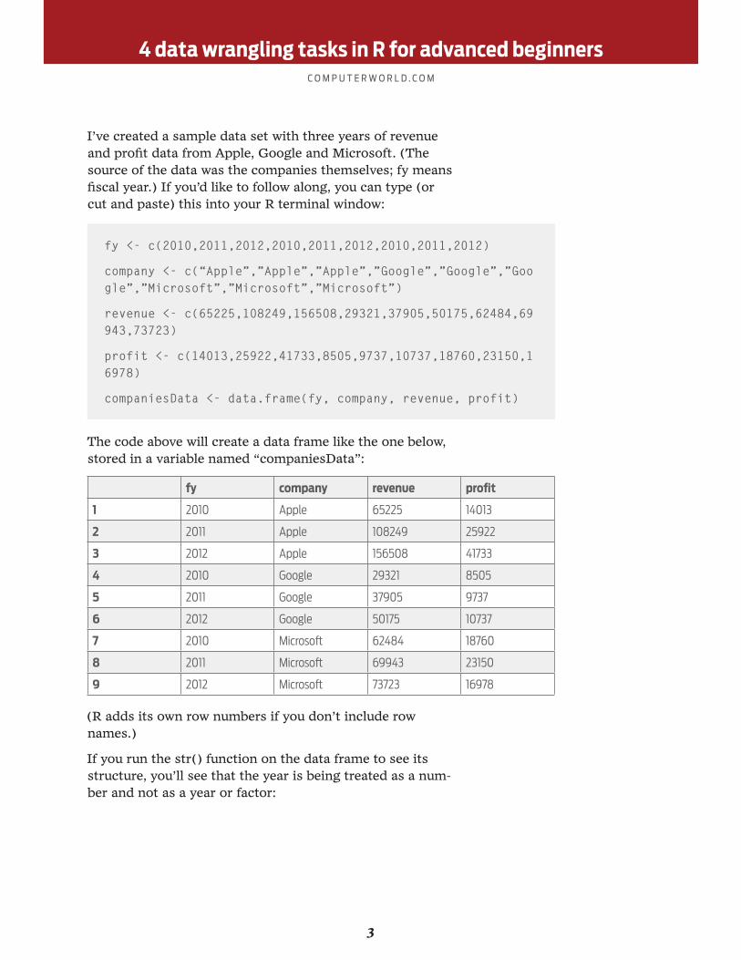
I’ve created a sample data set with three years of revenue and profit data from Apple, Google and Microsoft. (The source of the data was the companies themselves; fy means fiscal year.) If you’d like to follow along, you can type (or cut and paste) this into your R terminal window:

fy <- c(2010,2011,2012,2010,2011,2012,2010,2011,2012)

company <- c(“Apple”,”Apple”,”Apple”,”Google”,”Google”,”Google”,”Microsoft”,”Microsoft”,”Microsoft”)

revenue <- c(65225,108249,156508,29321,37905,50175,62484,69943,73723)

profit <- c(14013,25922,41733,8505,9737,10737,18760,23150,16978)

companiesData <- data.frame(fy, company, revenue, profit)

The code above will create a data frame like the one below, stored in a variable named “companiesData”:

fy company revenue profit

1 2010 Apple 65225 14013

2 2011 Apple 108249 25922

3 2012 Apple 156508 41733

4 2010 Google 29321 8505

5 2011 Google 37905 9737

6 2012 Google 50175 10737

7 2010 Microsoft 62484 18760

8 2011 Microsoft 69943 23150

9 2012 Microsoft 73723 16978

(R adds its own row numbers if you don’t include row names.)

If you run the str() function on the data frame to see its structure, you’ll see that the year is being treated as a num-ber and not as a year or factor:



4


str(companiesData)

‘data.frame’: 9 obs. of 4 variables:

$ fy : num 2010 2011 2012 2010 2011 ...

$ company: Factor w/ 3 levels “Apple”,”Google”,..: 1 1 1 2 2 2 3 3 3

$ revenue: num 65225 108249 156508 29321 37905 ...

$ profit : num 14013 25922 41733 8505 9737 ...

I may want to group my data by year, but don’t think I’m going to be doing specific time-based analysis, so I’ll turn the fy column of numbers into a column that contains R categories (called factors) instead of dates with the follow-ing command:

companiesData$fy <- factor(companiesData$fy, ordered = TRUE)

Now we’re ready to get to work.

Add a column to an existing data frameOne of the easiest tasks to perform in R is adding a new column to a data frame based on one or more other col-umns. You might want to add up several of your exist-ing columns, find an average or otherwise calculate some “result” from existing data in each row.

There are many ways to do this in R. Some will seem overly complicated for this easy task at hand, but for now you’ll have to take my word for it that some more complex options can come in handy for advanced users with more robust needs.

Syntax 1:

Simply create a variable name for the new column and pass in a calculation formula as its value if, for example, you want a new column that’s the sum of two existing columns:

dataFrame$newColumn <- dataFrame$oldColumn1 + dataFrame$oldColumn2



5


As you can probably guess, this creates a new column called “newColumn” with the sum of oldColumn1 + oldColumn2 in each row.

For our sample data frame called data, we could add a column for profit margin by dividing profit by revenue and then multiplying by 100:

companiesData$margin <- (companiesData$profit / companiesData$revenue) * 100

That gives us:

fy company revenue profit margin

1 2010 Apple 65225 14013 21.48409

2 2011 Apple 108248 25922 23.94664

3 2012 Apple 156508 41733 26.66509

4 2010 Google 29321 8505 29.00651

5 2011 Google 37905 9737 25.68790

6 2012 Google 50175 10737 21.39910

7 2010 Microsoft 62484 18760 30.02369

8 2011 Microsoft 69943 23150 33.09838

9 2012 Microsoft 73723 16978 23.02945

Whoa — that’s a lot of decimal places in the new margin column.

We can round that off to just one decimal place with the round() function; round() takes the format:

round(number(s) to be rounded, how many decimal places you want)

So, to round the margin column to one decimal place:

companiesData$margin <- round(companiesData$margin, 1)

And you’ll get this result:



6



1 2010 Apple 65225 14013 21.5

2 2011 Apple 108248 25922 23.9

3 2012 Apple 156508 41733 26.7

4 2010 Google 29321 8505 29.0

5 2011 Google 37905 9737 25.7

6 2012 Google 50175 10737 21.4

7 2010 Microsoft 62484 18760 30.0

8 2011 Microsoft 69943 23150 33.1

9 2012 Microsoft 73723 16978 23.0

Syntax 2: R’s transform() function

This is another way to accomplish what we did above. Here’s the basic transform() syntax:

dataFrame <- transform(dataFrame, newColumnName = some equation)

So, to get the sum of two columns and store that into a new column with transform(), you would use code such as:

dataFrame <- transform(dataFrame, newColumn = oldCol-umn1 + oldColumn2)

To add a profit margin column to our data frame with trans-form() we’d use:

companiesData <- transform(companiesData, margin = (profit/revenue) * 100)

We can then use the round() function to round the column results to one decimal place. Or, in one step, we can create a new column that’s already rounded to one decimal place:

companiesData <- transform(companiesData, margin = round((profit/revenue) * 100, 1))

One brief aside about round(): You can use negative num-bers for the second, “number of decimal places” argument. While round(73842.421, 1) will round to one decimal, in this case 73842.42, round(73842.421, -3) will round to the near-est thousand, in this case 74000.

Syntax 3: R’s apply() function

As the name helpfully suggests, this will apply a function to a data frame (or several other R data structures, but we’ll



7


stick with data frames for now). This syntax is more com-plicated than the first two but can be useful for some more complex calculations.

The basic format for apply() is:

dataFrame$newColumn <- apply(dataFrame, 1, function(x) { . . . } )

The line of code above will create a new column called “newColumn” in the data frame; the contents will be what-ever the code in { . . . } does.

Here’s what each of those apply() arguments above is doing. The first argument for apply() is the existing data frame. The second argument — 1 in this example — means “apply a function by row.” If that argument was 2, it would mean

“apply a function by column” — for example, if you wanted to get a sum or average by columns instead of for each row.

The third argument, function(x), should appear as written. More specifically the function( ) part needs to be written as just that; the “x” can be any variable name. This means

“What follows after this is an ad-hoc function that I haven’t named. I’ll call its input argument x.” What’s x in this case? It’s each item (row or column) being iterated over by apply().

Finally, { . . . } is whatever you want to be doing with each item you’re iterating over.

Keep in mind that apply() will seek to apply the function on every item in each row or column. That can be a problem if you’re applying a function that works only on numbers if some of your data frame columns aren’t numbers.

That’s exactly the case with our sample data of financial results. For the data variable, this won’t work:

apply(companiesData, 1, function(x) sum(x))

Why? Because (apply) will try to sum every item per row, and company names can’t be summed.

To use the apply() function on only some columns in the data frame, such as adding the revenue and profit columns together (which, I’ll admit, is an unlikely need in the real world of financial analysis), we’d need to use a subset of the data frame as our first argument. That is, instead of using apply() on the entire data frame, we just want apply() on the revenue and profit columns, like so:



8


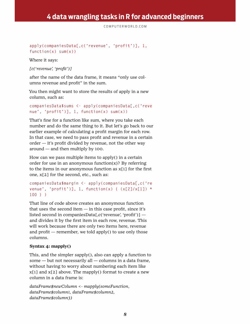
apply(companiesData[,c(‘revenue’, ‘profit’)], 1, function(x) sum(x))

Where it says:

[c(‘revenue’, ‘profit’)]

after the name of the data frame, it means “only use col-umns revenue and profit” in the sum.

You then might want to store the results of apply in a new column, such as:

companiesData$sums <- apply(companiesData[,c(‘revenue’, ‘profit’)], 1, function(x) sum(x))

That’s fine for a function like sum, where you take each number and do the same thing to it. But let’s go back to our earlier example of calculating a profit margin for each row. In that case, we need to pass profit and revenue in a certain order — it’s profit divided by revenue, not the other way around — and then multiply by 100.

How can we pass multiple items to apply() in a certain order for use in an anonymous function(x)? By referring to the items in our anonymous function as x[1] for the first one, x[2] for the second, etc., such as:

companiesData$margin <- apply(companiesData[,c(‘revenue’, ‘profit’)], 1, function(x) { (x[2]/x[1]) * 100 } )

That line of code above creates an anonymous function that uses the second item — in this case profit, since it’s listed second in companiesData[,c(‘revenue’, ‘profit’)] — and divides it by the first item in each row, revenue. This will work because there are only two items here, revenue and profit — remember, we told apply() to use only those columns.

Syntax 4: mapply()

This, and the simpler sapply(), also can apply a function to some — but not necessarily all — columns in a data frame, without having to worry about numbering each item like x[1] and x[2] above. The mapply() format to create a new column in a data frame is:

dataFrame$newColumn <- mapply(someFunction, dataFrame$column1, dataFrame$column2, dataFrame$column3)



9


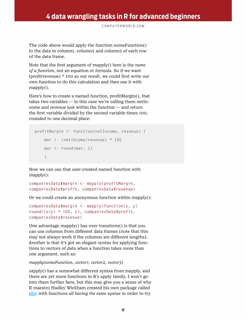
The code above would apply the function someFunction() to the data in column1, column2 and column3 of each row of the data frame.

Note that the first argument of mapply() here is the name of a function, not an equation or formula. So if we want (profit/revenue) * 100 as our result, we could first write our own function to do this calculation and then use it with mapply().

Here’s how to create a named function, profitMargin(), that takes two variables — in this case we’re calling them netIn-come and revenue just within the function — and return the first variable divided by the second variable times 100, rounded to one decimal place:

profitMargin <- function(netIncome, revenue) {

mar <- (netIncome/revenue) * 100

mar <- round(mar, 1)

}

Now we can use that user-created named function with mapply():

companiesData$margin <- mapply(profitMargin, companiesData$profit, companiesData$revenue)

Or we could create an anonymous function within mapply():

companiesData$margin <- mapply(function(x, y) round((x/y) * 100, 1), companiesData$profit, companiesData$revenue)

One advantage mapply() has over transform() is that you can use columns from different data frames (note that this may not always work if the columns are different lengths). Another is that it’s got an elegant syntax for applying func-tions to vectors of data when a function takes more than one argument, such as:

mapply(someFunction, vector1, vector2, vector3)

sapply() has a somewhat different syntax from mapply, and there are yet more functions in R’s apply family. I won’t go into them further here, but this may give you a sense of why R maestro Hadley Wickham created his own package called plyr with functions all having the same syntax in order to try


http://plyr.had.co.nz/


10


to rationalize applying functions in R. (We’ll get to plyr in the next section.)

For a more detailed look at base R’s various apply options, A brief introduction to ‘apply’ in R by bioinformatician Neil Saunders is a useful starting point.

Update: dplyr

Hadley Wickham’s dplyr package, released in early 2014 to rationalize and dramatically speed up operations on data frames, is another worthy option worth learning. To add a column to an existing data frame with dplyr, first install the package with install.packages(“dplyr”) — you only need to do this once — and then load it with library(“dplyr”). To add a column using dplyr:

companiesData <- mutate(companiesData, margin = round((profit/revenue) * 100, 1))

There will be more on the handy dplyr package to come.

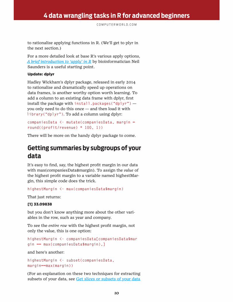
Getting summaries by subgroups of your dataIt’s easy to find, say, the highest profit margin in our data with max(companiesData$margin). To assign the value of the highest profit margin to a variable named highestMar-gin, this simple code does the trick.

highestMargin <- max(companiesData$margin)

That just returns:

[1] 33.09838

but you don’t know anything more about the other vari-ables in the row, such as year and company.

To see the entire row with the highest profit margin, not only the value, this is one option:

highestMargin <- companiesData[companiesData$margin == max(companiesData$margin),]

and here’s another:

highestMargin <- subset(companiesData, margin==max(margin))

(For an explanation on these two techniques for extracting subsets of your data, see Get slices or subsets of your data


http://nsaunders.wordpress.com/2010/08/20/a-brief-introduction-to-apply-in-r/

http://www.computerworld.com/article/2598083/app-development-beginner-s-guide-to-r-easy-ways-to-do-basic-data-analysis.html?page=4


11


from the Beginner’s guide to R: Easy ways to do basic data analysis.)

But what if you want to find rows with the highest profit margin for each company? That involves applying a function by groups — what R calls factors.

The plyr package created by Hadley Wickham considers this type of task “split-apply-combine”: Split up your data set by one or more factors, apply some function, then com-bine the results back into a data set.

plyr’s ddply() function performs a “split-apply-combine” on a data frame and then produces a new separate data frame with your results. That’s what the first two letters, dd, stand for in ddply(), by the way: Input a data frame and get a data frame back. There’s a whole group of “ply” functions in the plyr package: alply to input an array and get back a list, ldply to input a list and get back a data frame, and so on.

To use ddply(), first you need to install the plyr package if you never have, with:

install.packages(“plyr”)

Then, if you haven’t yet for your current R session, load the plyr package with:

library(“plyr”)

The format for splitting a data frame by multiple factors and applying a function with ddply would be:

ddply(mydata, c(‘column name of a factor to group by’, ‘col-umn name of the second factor to group by’), summarize OR transform, newcolumn = myfunction(column name(s) I want the function to act upon))

Let’s take a more detailed look at that. The ddply() first argument is the name of the original data frame and the second argument is the name of the column or columns you want to subset your data by. The third tells ddply() whether to return just the resulting data points (summarize) or the entire data frame with a new column giving the desired data point per factor in every row. Finally, the fourth argu-ment names the new column and then lists the function you want ddply() to use.

If you don’t want to have to put the column names in quotes, an alternate syntax you’ll likely see frequently uses a dot before the column names:


http://www.computerworld.com/article/2598083/app-development-beginner-s-guide-to-r-easy-ways-to-do-basic-data-analysis.html

http://www.computerworld.com/article/2598083/app-development-beginner-s-guide-to-r-easy-ways-to-do-basic-data-analysis.html


12


myresult <- ddply(mydata, .(column name of factor I’m split-ting by, column name second factor I’m splitting by), summa-rize OR transform, newcolumn = myfunction(column name I want the function to act upon))

To get the highest profit margins for each company, we’re splitting the data frame by only one factor — company. To get just the highest value and company name for each com-pany, use summarize as the third argument:

highestProfitMargins <- ddply(companiesData, .(company), summarize, bestMargin = max(margin))

(Here we’ve assigned the results to the variable highestProfitMargins.)

Syntax note: Even if you’ve only got one factor, it needs to be in parentheses after that dot if you’re using the dot to avoid putting the column name in quotes. No parentheses are needed for just one factor if you’re using quotation marks:

highestProfitMargins <- ddply(companiesData, ‘company’, summarize, bestMargin = max(margin))

Either way, you’ll end up with a brand new data frame with the highest profit margin for each company:

company bestMargin

1 Apple 26.7

2 Google 29.0

3 Microsoft 33.1

Summarize doesn’t give any information from other col-umns in the original data frame. In what year did each of the highest margins occur? We can’t tell by using summarize.

If you want all the other column data, too, change “sum-marize” to “transform.” That will return your existing data frame with a new column that repeats the maximum margin for each company:

highestProfitMargins <- ddply(companiesData, ‘company’, transform, bestMargin = max(margin))



13


fy company revenue profit margin bestMar-gin

1 2010 Apple 65225 14013 21.5 26.7

2 2011 Apple 108248 25922 23.9 26.7

3 2012 Apple 156508 41733 26.7 26.7

4 2010 Google 29321 8505 29.0 29.0

5 2011 Google 37905 9737 25.7 29.0

6 2012 Google 50175 10737 21.4 29.0

7 2010 Microsoft 62484 18760 30.0 33.1

8 2011 Microsoft 69943 23150 33.1 33.1

9 2012 Microsoft 73723 16978 23.0 33.1

Note that this result shows the profit margin for each com-pany and year in the margin column along with the best-Margin repeated for each company and year. The only way to tell which year has the best margin is to compare the two columns to see where they’re equal.

ddply() lets you apply more than one function at a time, for example:

myResults <- ddply(companiesData, ‘company’, transform, highestMargin = max(margin), lowestMargin = min(margin))

This gets you:

fy company revenue profit margin highest-Margin

lowestMar-gin

1 2010 Apple 65225 14013 21.5 26.7 21.5

2 2011 Apple 108248 25922 23.9 26.7 21.5

3 2012 Apple 156508 41733 26.7 26.7 21.5

4 2010 Google 29321 8505 29.0 29.0 21.4

5 2011 Google 37905 9737 25.7 29.0 21.4

6 2012 Google 50175 10737 21.4 29.0 21.4

7 2010 Microsoft 62484 18760 30.0 33.1 23.0

8 2011 Microsoft 69943 23150 33.1 33.1 23.0

9 2012 Microsoft 73723 16978 23.0 33.1 23.0

In some cases, though, what you want is a new data frame with just the (entire) rows that have the highest profit mar-



14


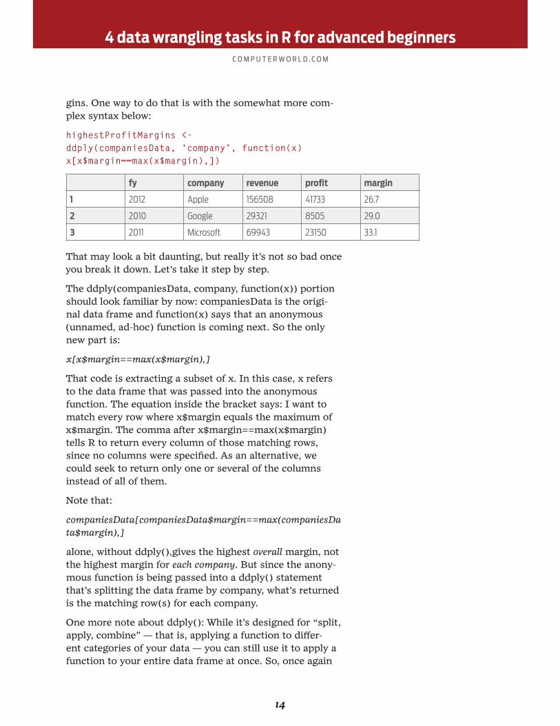
gins. One way to do that is with the somewhat more com-plex syntax below:

highestProfitMargins <- ddply(companiesData, ‘company’, function(x) x[x$margin==max(x$margin),])


1 2012 Apple 156508 41733 26.7

2 2010 Google 29321 8505 29.0

3 2011 Microsoft 69943 23150 33.1

That may look a bit daunting, but really it’s not so bad once you break it down. Let’s take it step by step.

The ddply(companiesData, company, function(x)) portion should look familiar by now: companiesData is the origi-nal data frame and function(x) says that an anonymous (unnamed, ad-hoc) function is coming next. So the only new part is:

x[x$margin==max(x$margin),]

That code is extracting a subset of x. In this case, x refers to the data frame that was passed into the anonymous function. The equation inside the bracket says: I want to match every row where x$margin equals the maximum of x$margin. The comma after x$margin==max(x$margin) tells R to return every column of those matching rows, since no columns were specified. As an alternative, we could seek to return only one or several of the columns instead of all of them.

Note that:

companiesData[companiesData$margin==max(companiesData$margin),]

alone, without ddply(),gives the highest overall margin, not the highest margin for each company. But since the anony-mous function is being passed into a ddply() statement that’s splitting the data frame by company, what’s returned is the matching row(s) for each company.

One more note about ddply(): While it’s designed for “split, apply, combine” — that is, applying a function to differ-ent categories of your data — you can still use it to apply a function to your entire data frame at once. So, once again



15


here’s the ddply() statement we used to get a summary of highest profit margin for each company:

highestProfitMargins <- ddply(companiesData, ‘company’, summarize, bestMargin = max(margin))

To use ddply() to see the highest margin in the entire data set, not just segmented by company, I’d enter NULL as the second argument for factors to split by:

highestProfitMargin <- ddply(companiesData, NULL, summarize, bestMargin = max(margin))

That’s obviously a much more complicated way of doing this than max(companiesData$margin). But you neverthe-less may find plyr’s “ply” family useful at times if you want to apply multiple functions on an entire data structure and like the idea of consistent syntax.

Update with dplyr: Performing these operations with dplyr is considerably faster than with plyr — not an issue for a tiny data frame like this, but important if you’ve got data with thousands of rows. In addition, dplyr syntax is more read-able and intuitive — once you get used to it.

To add the two columns for highest and lowest margins by company:

myresults <- companiesData %>%

group_by(company) %>%

mutate(highestMargin = max(margin), lowestMargin = min(margin))

and to create a new data frame with maximum margin by company:

highestProfitMargins <- companiesData %>%

group_by(company) %>%

summarise(bestMargin = max(margin))

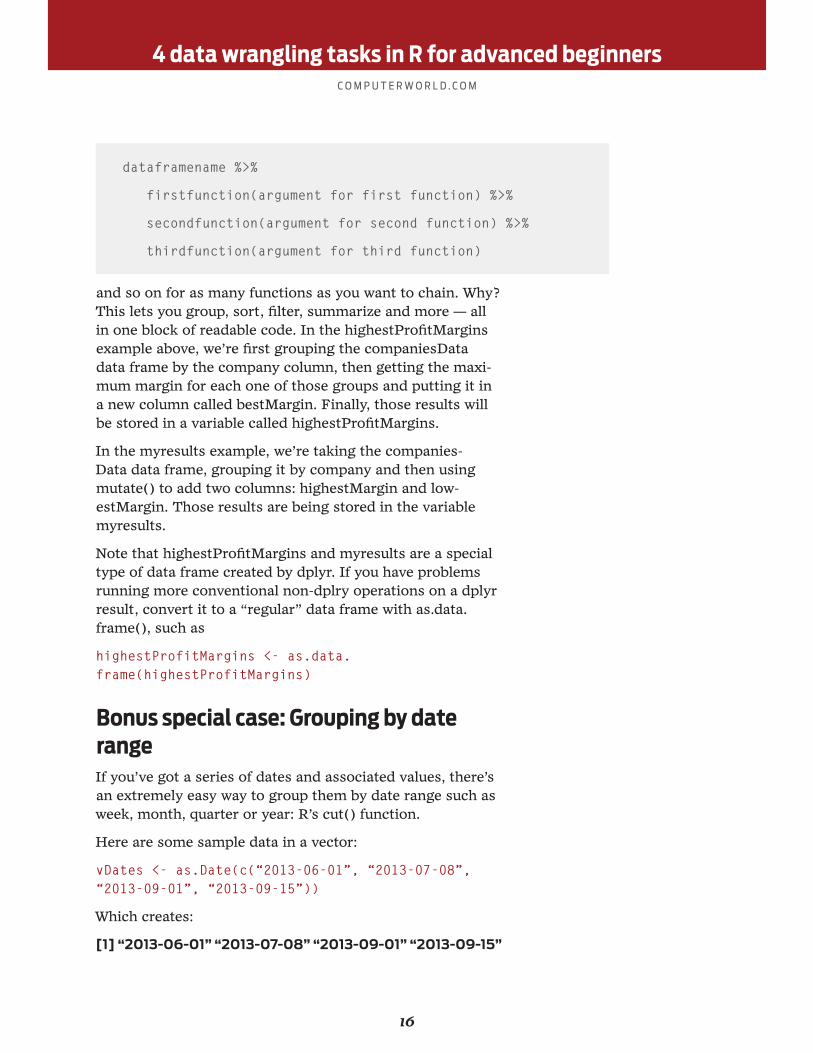
The %>% is a “chaining” operation that allows you to string together multiple commands on a data frame. The chaining syntax in general is:



16


dataframename %>%

firstfunction(argument for first function) %>%

secondfunction(argument for second function) %>%

thirdfunction(argument for third function)

and so on for as many functions as you want to chain. Why? This lets you group, sort, filter, summarize and more — all in one block of readable code. In the highestProfitMargins example above, we’re first grouping the companiesData data frame by the company column, then getting the maxi-mum margin for each one of those groups and putting it in a new column called bestMargin. Finally, those results will be stored in a variable called highestProfitMargins.

In the myresults example, we’re taking the companies-Data data frame, grouping it by company and then using mutate() to add two columns: highestMargin and low-estMargin. Those results are being stored in the variable myresults.

Note that highestProfitMargins and myresults are a special type of data frame created by dplyr. If you have problems running more conventional non-dplry operations on a dplyr result, convert it to a “regular” data frame with as.data.frame(), such as

highestProfitMargins <- as.data.frame(highestProfitMargins)

Bonus special case: Grouping by date rangeIf you’ve got a series of dates and associated values, there’s an extremely easy way to group them by date range such as week, month, quarter or year: R’s cut() function.

Here are some sample data in a vector:

vDates <- as.Date(c(“2013-06-01”, “2013-07-08”, “2013-09-01”, “2013-09-15”))

Which creates:

[1] “2013-06-01” “2013-07-08” “2013-09-01” “2013-09-15”



17


The as.Date() function is important here; otherwise R will view each item as a string object and not a date object.

If you want a second vector that sorts those by month, you can use the cut() function using the basic syntax:

vDates.bymonth <- cut(vDates, breaks = “month”)

That produces:

[1] 2013-06-01 2013-07-01 2013-09-01 2013-09-01

Levels: 2013-06-01 2013-07-01 2013-08-01 2013-09-01

It might be easier to see what’s happening if we combine these into a data frame:

dfDates <- data.frame(vDates, vDates.bymonth)

Which creates:

vDates vDates.bymonth

1 2013-06-01 2013-06-01

2 2013-07-08 2013-07-01

3 2013-09-01 2013-09-01

4 2013-09-15 2013-09-01

The new column gives the starting date for each month, making it easy to then slice by month.

Ph.D. student Mollie Taylor’s blog post Plot Weekly or Monthly Totals in R introduced me to this shortcut, which isn’t apparent if you simply read the cut() help file. If you ever work with analyzing and plotting date-based data, this short and extremely useful post is definitely worth a read. Her downloadable code is available as a GitHub gist.

Sorting your resultsFor a simple sort by one column, you can get the order you want with the order() function, such as:

companyOrder <- order(companiesData$margin)

This tells you how your rows would be reordered, producing a list of line numbers such as:

6 1 9 2 5 3 4 7 8

Chances are, you’re not interested in the new order by line number but instead actually want to see the data reordered.


http://www.mollietaylor.com/2013/08/plot-weekly-or-monthly-totals-in-r.html

http://www.mollietaylor.com/2013/08/plot-weekly-or-monthly-totals-in-r.html

https://gist.github.com/mollietaylor/5846843


18


You can use that order to reorder rows in your data frame with this code:

companiesOrdered <- companiesData[companyOrder,]

where companyOrder is the order you created earlier. Or, you can do this in a single (but perhaps less human-read-able) line of code:

companiesOrdered <- companiesData[order(companiesData$margin),]

If you forget that comma after the new order for your rows you’ll get an error, because R needs to know what columns to return. Once again, a comma followed by noth-ing defaults to “all columns” but you can also specify just certain columns like:

companiesOrdered <- companiesData[order(companiesData$margin),c(“fy”, “company”)]

To sort in descending order, you’d want companyOrder to have a minus sign before the ordering column:

companyOrder <- order(-companiesData$margin)

And then:

companiesOrdered <- companiesData[companyOrder,]

You can put that together in a single statement as:

companiesOrdered <- companiesData[order(-companiesData$margin),]


8 2011 Microsoft 69943 23150 33.1

7 2010 Microsoft 62484 18760 30.0

4 2010 Google 29321 8505 29.0

3 2012 Apple 156508 41733 26.7

5 2011 Google 37905 9737 25.7

2 2011 Apple 108249 25922 23.9

9 2012 Microsoft 73723 16978 23.0

1 2010 Apple 65225 14013 21.5

6 2012 Google 50175 10737 21.4

Note how you can see the original row numbers reordered at the far left.



19


If you’d like to sort one column ascending and another col-umn descending, just put a minus sign before the one that’s descending. This is one way to sort this data first by year (ascending) and then by profit margin (descending) to see which company had the top profit margin by year:

companiesData[order(companiesData$fy, -companiesData$margin),]

If you don’t want to keep typing the name of the data frame followed by the dollar sign for each of the column names, R’s with() function takes the name of a data frame as the first argument and then lets you leave it off in subsequent arguments in one command:

companiesOrdered <- companiesData[with(companiesData, order(fy, -margin)),]

While this does save typing, it can make your code some-what less readable, especially for less experienced R users.

Packages offer some more elegant sorting options. The doBy package features orderBy() using the syntax

orderBy(~columnName + secondColumnName, data=dataFrameName)

The ~ at the beginning just means “by” (as in “order by this”). If you want to order by descending, just put a minus sign after the tilde and before the column name. This also orders the data frame:

companiesOrdered <- orderBy(~-margin, companiesData)

Both plyr and dplyr have an arrange() function with the syntax

arrange(dataFrameName, columnName, secondColumnName)

To sort descending, use desc(columnName))

companiesOrdered <- arrange(companiesData, desc(margin))

Reshaping: Wide to long (and back)Different analysis tools in R — including some graphing packages — require data in specific formats. One of the most common — and important — tasks in R data manipu-



20


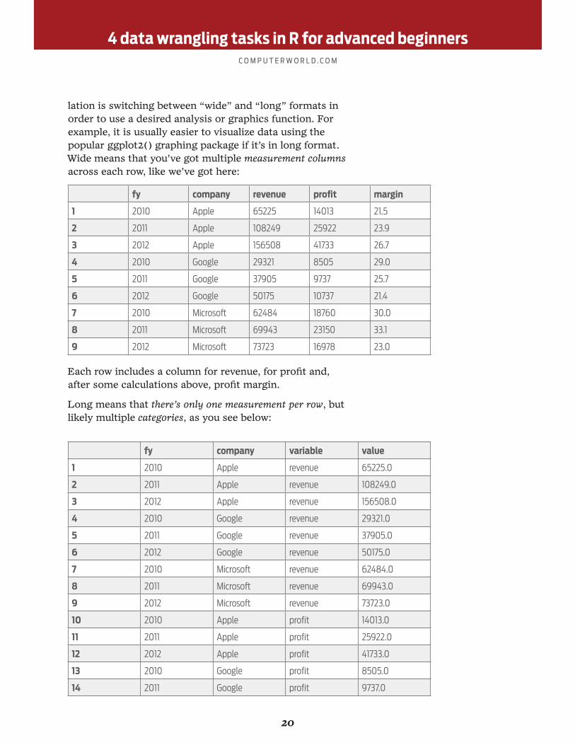
lation is switching between “wide” and “long” formats in order to use a desired analysis or graphics function. For example, it is usually easier to visualize data using the popular ggplot2() graphing package if it’s in long format. Wide means that you’ve got multiple measurement columns across each row, like we’ve got here:


1 2010 Apple 65225 14013 21.5

2 2011 Apple 108249 25922 23.9

3 2012 Apple 156508 41733 26.7

4 2010 Google 29321 8505 29.0

5 2011 Google 37905 9737 25.7

6 2012 Google 50175 10737 21.4

7 2010 Microsoft 62484 18760 30.0

8 2011 Microsoft 69943 23150 33.1

9 2012 Microsoft 73723 16978 23.0

Each row includes a column for revenue, for profit and, after some calculations above, profit margin.

Long means that there’s only one measurement per row, but likely multiple categories, as you see below:

fy company variable value

1 2010 Apple revenue 65225.0



4 2010 Google revenue 29321.0



7 2010 Microsoft revenue 62484.0



10 2010 Apple profit 14013.0

11 2011 Apple profit 25922.0

12 2012 Apple profit 41733.0

13 2010 Google profit 8505.0




21



16 2010 Microsoft profit 18760.0



19 2010 Apple margin 21.5



22 2010 Google margin 29.0



25 2010 Microsoft margin 30.0



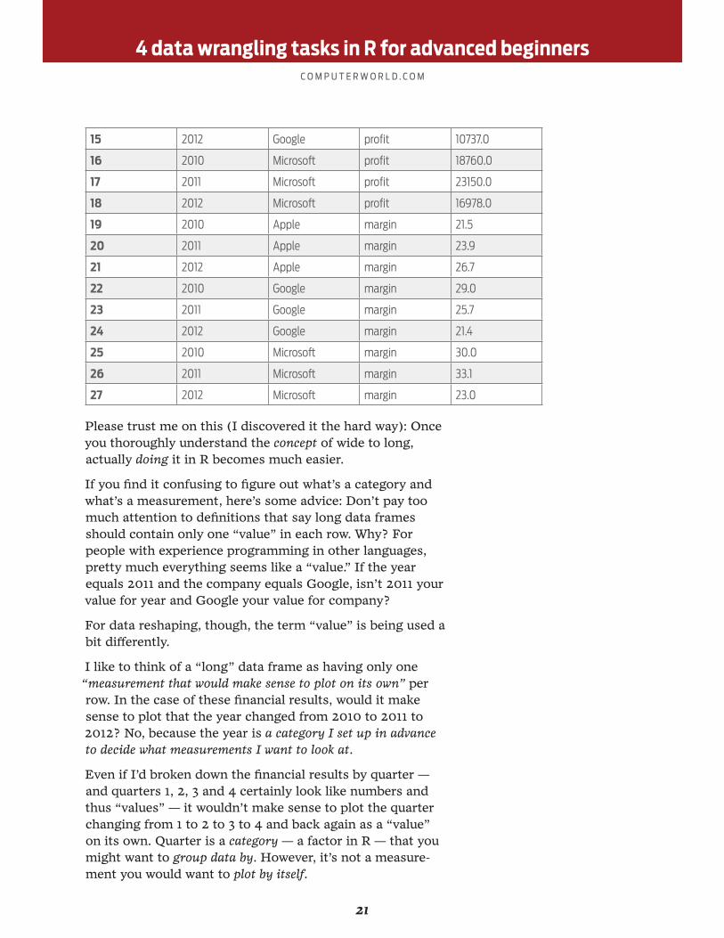
Please trust me on this (I discovered it the hard way): Once you thoroughly understand the concept of wide to long, actually doing it in R becomes much easier.

If you find it confusing to figure out what’s a category and what’s a measurement, here’s some advice: Don’t pay too much attention to definitions that say long data frames should contain only one “value” in each row. Why? For people with experience programming in other languages, pretty much everything seems like a “value.” If the year equals 2011 and the company equals Google, isn’t 2011 your value for year and Google your value for company?

For data reshaping, though, the term “value” is being used a bit differently.

I like to think of a “long” data frame as having only one “measurement that would make sense to plot on its own” per row. In the case of these financial results, would it make sense to plot that the year changed from 2010 to 2011 to 2012? No, because the year is a category I set up in advance to decide what measurements I want to look at.

Even if I’d broken down the financial results by quarter — and quarters 1, 2, 3 and 4 certainly look like numbers and thus “values” — it wouldn’t make sense to plot the quarter changing from 1 to 2 to 3 to 4 and back again as a “value” on its own. Quarter is a category — a factor in R — that you might want to group data by. However, it’s not a measure-ment you would want to plot by itself.



22


This may be more apparent in the world of scientific experi-mentation. If you’re testing a new cholesterol drug, for example, the categories you set up in advance might look at patients by age, gender and whether they’re given the drug or a placebo. The measurements (or calculations resulting from those measurements) are your results: Changes in overall cholesterol level, LDL and HDL, for example. But whatever your data, you should have at least one category and one measurement if you want to create a long data frame.

In the example data we’ve been using here, my categories are fy and company, while my measurements are revenue, profit and margin.

And now here’s the next concept you need to understand about reshaping from wide to long: Because you want only one measurement in each row, you need to add a column that says which type of measurement each value is.

In my existing wide format, the column headers tell me the measurement type: revenue, profit or margin. But since I’m rearranging this to only have one of those numbers in each row, not three, I’ll add a column to show which measure-ment it is.

I think an example will make this a lot clearer. Here’s one “wide” row:


2010 Apple 65225 14013 21.48409

And here’s how to have only one measurement per row — by creating three “long” rows:

fy company financialCategory value

2010 Apple revenue 65225

2010 Apple profit 14013

2010 Apple margin 21.5

The column financialCategory now tells me what type of measurement each value is. And now, the term “value” should make more sense.

At last we’re ready for some code to reshape a data frame from wide to long! As with pretty much everything in R, there are multiple ways to perform this task. To use



23


reshape2, first you need to install the package if you never have, with:

install.packages(“reshape2”)

Load it with:

library(reshape2)

And then use reshape2’s melt() function. melt() uses the following format to assign results to a variable named longData:

longData <- melt(your original data frame, a vector of your category variables)

That’s all melt() requires: The name of your data frame and the names of your category variables. However, you can optionally add several other variables, including a vector of your measurement variables (if you don’t, melt() assumes that all the rest of the columns are measurement columns) and the name you want your new category column to have.

So, again using the data frame of sample data, wide-to-long code can simply be:

companiesLong <- melt(companiesData, c(“fy”, “company”))

This produces:

fy company variable value










10 2010 Apple profit 14013.0

11 2011 Apple profit 25922.0

12 2012 Apple profit 41733.0





24















It’s actually fairly simple after you understand the basic concept. Here, the code assumes that all the other columns except fy and company are measurements — items you might want to plot.

You can be lengthier in your code if you prefer, especially if you think that will help you remember what you did down the road. The statement below lists all the column in the data frame, assigning them to either id.vars or measure.vars, and also changes the new column names from the default

“variable” and “value”:

I find it a bit confusing that reshape2 calls category vari-ables “id.vars” (short for ID variables) and not categories or factors, but after a while you’ll likely get used to that. Mea-surement variables in reshape2 are somewhat more intui-tively called measure.vars.

companiesLong <- melt(companiesData, id.vars=c(“fy”, “company”), measure.vars=c(“revenue”, “profit”, “margin”), variable.name=”financialCategory”, value.name=”amount”)

This produces:



25


fy company financialCat-egory

amount










10 2010 Apple profit 14013.0

11 2011 Apple profit 25922.0

12 2012 Apple profit 41733.0
















Reshaping: Long to wideOnce your data frame is “melted,” it can be “cast” into any shape you want. reshape2’s dcast() function takes a “long” data frame as input and allows you to create a reshaped data frame in return. (The somewhat similar acast() func-tion can return an array, vector or matrix.) One of the best



26


explanations I’ve seen on going from long to wide with dcast() is from the R Graphics Cookbook by Winston Chang:

“[S]pecify the ID variables (those that remain in col-umns) and the variable variables (those that get

‘moved to the top’). This is done with a formula where the ID variables are before the tilde (~) and the variable variables are after it.”

In other words, think briefly about the structure you want to create. The variables you want repeating in each row are your “ID variables.” Those that should become column headers are your “variable variables.”

Look at this row from the original, “wide” version of our table:


2010 Apple 65225 14013 21.5

Everything following fiscal year and company is a measure-ment relating to that specific year and company. That’s why fy and company are the ID variables; while revenue, profit and margin are the “variable variables” that have been

“moved to the top” as column headers.

How to re-create a wide data frame from the long version of the data? Here’s code, if you’ve got two columns with ID variables and one column with variable variables:

wideDataFrame <- dcast(longDataFrame, idVariableColumn1 + idVariableColumn2 ~ variableColumn, value.var=”Name of column with the measurement values”)

dcast() takes the name of a long data frame as the first argument. You need to create a formula of sorts as the sec-ond argument with the syntax:

id variables ~ variable variables

The id and measurement variables are separated by a tilde, and if there are more than one on either side of the tilde they are listed with a plus sign between them.

The third argument for dcast() assigns the name of the col-umn that holds your measurement values to value.var.

So, to produce the original, wide data frame from compa-niesLong using dcast():


http://shop.oreilly.com/product/0636920023135.do


27


companiesWide <- dcast(companiesLong, fy + company ~ financialCategory, value.var=”amount”)

To break that down piece by piece: companiesLong is the name of my long data frame; fy and company are the col-umns I want to remain as items in each row of my new, wide data frame; I want to create a new column for each of the different categories in the financialCategory column — move them up to the top to become column headers, as Chang said; and I want the actual measurements for each of those financial categories to come from the amount column.

Update: Hadley Wickham created the tidyr package to per-form a subset of reshape2’s capabilities with two main func-tions: gather() to take multiple values and turn them into key-value pairs and spread() to go from long to wide. I still use reshape2 for these tasks, but you may find tidyr better fits your needs.

Wrap-upHopefully instructions for these data-wrangling tasks have helped you solve a particular problem and/or continue on the journey of mastering R for data work. To learn more about R, see Computerworld’s 60+ R resources to improve your data skills.


https://github.com/hadley/tidyr

http://www.computerworld.com/article/2497464/business-intelligence-60-r-resources-to-improve-your-data-skills.html

http://www.computerworld.com/article/2497464/business-intelligence-60-r-resources-to-improve-your-data-skills.html

4 data wrangling tasks in r for advanced beginnersduspviz.mit.edu/resources/r/r for advanced...

Documents