3D Tomographic Study of Mid-latitude Sporadic-E Irregularities

in Japan from GNSS-TEC Data

by

Ihsan Naufal Muafiry

A thesis submitted in partial fulfillment

of the requirements for the degree

of Master of Science

2

Table of Contents

Acknowledgements .................................................................................................................. 3

Abstract ..................................................................................................................................... 5

Chapter 1 .................................................................................................................................. 7

1.1 Sporadic-E .......................................................................................................................... 7

1.2. Total Electron Content (TEC) ............................................................................................. 8

1.3. GNSS-TEC technique ......................................................................................................... 9

1.4. Ionosphere 3D Tomography.............................................................................................. 10

Chapter 2 ................................................................................................................................ 12

2.1. Dataset............................................................................................................................... 12

2.2. Method .............................................................................................................................. 12

Chapter 3 ................................................................................................................................ 17

3.1. Resolution tests ................................................................................................................. 17

3.2. Multi GNSS assessment and finding the best constraint .................................................. 21

Chapter 4 ................................................................................................................................ 25

4.1. Es 3D-Tomography result ................................................................................................. 25

4.2. Horizontal drift of Es patches and its vertical structure .................................................... 27

4.3. Accuracy of tomography result ......................................................................................... 28

Chapter 5 ................................................................................................................................ 31

5.1. Conclusions ....................................................................................................................... 31

References ............................................................................................................................... 32

3

Acknowledgements

First of all, I praise to Allah subhanahuwata’ala for the things He has given to me.

Since this two years period of my study is not only a journey of achieving a higher degree,

but also is becoming my greatest experience ever in my life. Indeed, the second place for all

of these, I would acknowledge my parents who have always been supporting and praying for

me to go further just for the sake of knowledge. Third place is without a doubt, I thank to my

little family (my wife and my son) who have been accompanying and supporting my journey

in Japan as well as coloring my new life.

Over the last couple of years, an incredible number of people have been helping me a

lot in my journey. They deserve the gratitude of a thousand pages. First, I would like to

express my sincere gratitude to Prof. Kosuke Heki, my supervisor, who has given me

opportunity to become a great and smart researcher. I learned many lessons and all of those

are really valuable for my carrier path. He taught me about programming with its technical

aspects, making a presentation, presenting slides, writing a scientific paper, and gave me

chances to speak at international conferences. Sensei inspires me, and I could not have

written this thesis without that inspiration. Thanks again sensei as always.

My sincere gratitude to Prof. Masato Furuya, Prof. Kiyoshi Yomogida, Prof. Kazunori

Yoshizawa, and Dr. Yoichiro Takada for the advices delivered to my study during weekly

solid-earth science seminar or after the seminar. Those are definitely encouraging me to

become better and better in scientific field. Also, my colleagues at Space Geodesy and

Seismology Laboratories. I received many new perspectives of earth-sciences after discussing

with them.

To Geospatial Survey Information Authority of Japan (GSI) for providing GNSS data

from GEONET online. Thank you very much. And finally, to Indonesian Endowment Fund

for Education (LPDP) who supports me financially during my master study in Hokkaido

4

University. A huge thank you to directors, LPDP’s staffs and all elements for accepting and

supporting me as an awardee.

5

Abstract

Three-dimensional (3D) structures of five midlatitude sporadic-E (Es) ionospheric

irregularities are studied by using total electron content (TEC) observations with a dense

array of Global Navigation Positoning System (GNSS) in Japan called GEONET (GNSS

Earth Observation Network). Here I follow pioneering studies of Es in 2D method and

analyze the 3D structures of several cases.

In Chapter 2, we try to apply the 3D tomography technique as a new method for Es

cases studied earlier over the Kanto and Kyushu Districts, Japan. We used the slant TEC

residuals from reference curves as the input, and estimated the electron density anomalies

within >2000 small blocks with dimensions of 20-30 kilometers covering the region as large

as 300 x 500 km. We applied a continuity constraint to stabilize the solution, and performed

resolution tests with synthetic data, to assess the accuracy of the results.

In Chapter 3, I show the results of the two kinds of reliability test. First is the classical

checkerboard-test and the second is the test by assuming a realistic Es-like anomaly pattern. I

assumed that horizontal structure of our tomography result can be recovered pretty well

above the land area, but resolution is not good above ocean region and at high altitudes. I

found serious smearings in the latitudinal-height sections, which implies that we should be

careful in discussing the 3D structures of Es patches based on our tomography results. Here I

also discuss the impact of using multi GNSS on the quality of the solution.

In Chapter 4, I study three dimention morphological characteristics of Es patches. The

tomography results showed that the positive electron density anomalies occured at the E

region height, ~100 km above ground, with morphology and dynamics consistent with earlier

studies. Assessment to the accuracy of the tomography results is done by two statistical

approaches, i.e. by looking at the formal errors and by comparing the raw observation data

6

with the post-fit residuals. We confirmed that our tomography has the best accuracy on land

and at lower heights.

7

Chapter 1

1.1 Sporadic-E

Sporadic-E (Es) occurs as a patch of thin layer of anomalously high ionization at altitudes

~100 km (E-region) of the Earth’s ionosphere. It causes irregular long-distance propagation

of radio signals and often degrade the navigation accuracy of Global Navigation Satellite

System (GNSS). Es occurs at low-latitude (Jayachandran et al., 1999; Resende and Denardini,

2012), mid-latitude (Maeda and Heki, 2014; Wakabayashi et al., 2005), and high-latitude

(Kirkwood and Nilsson, 2000) regions, and is widely believed to be generated by the vertical

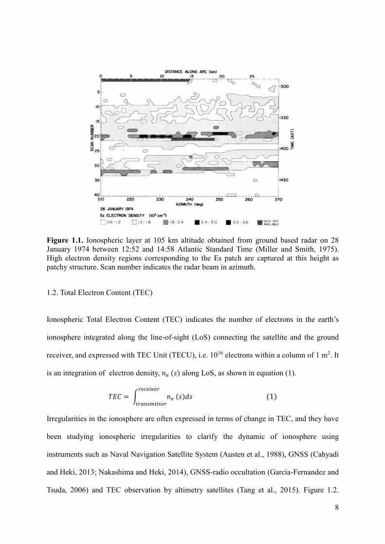
shear of zonal winds (Whitehead, 1970). Ground-based radars, such as ionosonde, revealed

that Es irregularities have horizontally patchy structures (Figure 1.1) done by Miller and

Smith (1975, 1978).

In addition to studies with numerical simulation approaches (Yokoyama et al., 2005),

sounding rockets were launched to the height of several hundred kilometers to study Es

(Yamamoto and Ono, 1998; Wakabayashi et al., 2005; Bernhardt et al., 2005; Kurihara et al.,

2010). Using a magnesium ion imager on-board a rocket, Kurihara et al. (2010) succesfully

imaged the patchy frontal structures of Es by scanning the magnesium ion distribution within

the layer.

Maeda & Heki (2014; 2015) used the dense array made of ~1200 GNSS receivers in

Japan, GEONET (GNSS Earth Observation Network), and to reveal the horizontal structure

and time evolution of daytime Es irregularities over Japan. They found that Es patches with

foEs (frequency of Es) exceeding 20 MHz present clear signatures in GNSS-TEC data,

recognized as short-term localized enhancements in TEC. They found that Es usually shows

frontal structure extending hundreds of kilometers dominantly in east-west. A dramatic

improvement in spatial resolution, furthermore, has been realized by joint observations of Es

with GNSS and interferometric Synthetic Aperture Radar (InSAR) (Maeda et al., 2016).

8

Figure 1.1. Ionospheric layer at 105 km altitude obtained from ground based radar on 28

January 1974 between 12:52 and 14:58 Atlantic Standard Time (Miller and Smith, 1975).

High electron density regions corresponding to the Es patch are captured at this height as

patchy structure. Scan number indicates the radar beam in azimuth.

1.2. Total Electron Content (TEC)

Ionospheric Total Electron Content (TEC) indicates the number of electrons in the earth’s

ionosphere integrated along the line-of-sight (LoS) connecting the satellite and the ground

receiver, and expressed with TEC Unit (TECU), i.e. 1016 electrons within a column of 1 m2. It

is an integration of electron density, 𝑛𝑒 (𝑠) along LoS, as shown in equation (1).

𝑇𝐸𝐶 = ∫ 𝑛𝑒 (𝑠)𝑑𝑠 (1)𝑟𝑒𝑐𝑒𝑖𝑣𝑒𝑟

𝑡𝑟𝑎𝑛𝑠𝑚𝑖𝑡𝑡𝑒𝑟

Irregularities in the ionosphere are often expressed in terms of change in TEC, and they have

been studying ionospheric irregularities to clarify the dynamic of ionosphere using

instruments such as Naval Navigation Satellite System (Austen et al., 1988), GNSS (Cahyadi

and Heki, 2013; Nakashima and Heki, 2014), GNSS-radio occultation (Garcia-Fernandez and

Tsuda, 2006) and TEC observation by altimetry satellites (Tang et al., 2015). Figure 1.2.

9

shows the GNSS-TEC technique.

Figure 1.2. An illustration showing the concept of the GNSS-TEC technique. It measures

number of electrons integrated along the LoS connecting the satellite and the ground receiver.

1.3. GNSS-TEC technique

GNSS-TEC technique is now extensively used for sounding the ionosphere penetrated

by LoS connecting the satellites and the stations. The pioneering work of this method was

done by Calais and Minster (1995), who studied ionospheric perturbations by an earthquake.

Further explanations of this method will be given in Chapter 2.

The original purpose of GNSS is not ionospheric observations but crustal deformation

studies. Nevertheless, GNSS-TEC technique has increased the versatility of GNSS as a multi-

purpose tool. Numbers of papers have been published using this method to investigate

ionospheric disturbances. They include those by volcanic eruptions, e.g. Heki (2006) and

Dautermann et al. (2009). They observed atmospheric waves reaching ionosphere right after

the 2004 explosion of the Asama Volcano, Central Japan, and the 2009 eruption of the

Soufriere Hills volcano, in the Lesser Antilles, respectively. Targets of the GNSS-TEC studies

also include human-induced phenomena such as Ozeki and Heki (2010) and Nakashima and Heki

(2014). They focused on the change of ionospheric TEC before and after the launches of ballistic

10

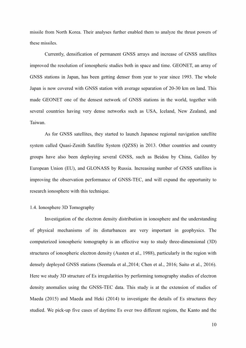
missile from North Korea. Their analyses further enabled them to analyze the thrust powers of

these missiles.

Currently, densification of permanent GNSS arrays and increase of GNSS satellites

improved the resolution of ionospheric studies both in space and time. GEONET, an array of

GNSS stations in Japan, has been getting denser from year to year since 1993. The whole

Japan is now covered with GNSS station with average separation of 20-30 km on land. This

made GEONET one of the densest network of GNSS stations in the world, together with

several countries having very dense networks such as USA, Iceland, New Zealand, and

Taiwan.

As for GNSS satellites, they started to launch Japanese regional navigation satellite

system called Quasi-Zenith Satellite System (QZSS) in 2013. Other countries and country

groups have also been deploying several GNSS, such as Beidou by China, Galileo by

European Union (EU), and GLONASS by Russia. Increasing number of GNSS satellites is

improving the observation performance of GNSS-TEC, and will expand the opportunity to

research ionosphere with this technique.

1.4. Ionosphere 3D Tomography

Investigation of the electron density distribution in ionosphere and the understanding

of physical mechanisms of its disturbances are very important in geophysics. The

computerized ionospheric tomography is an effective way to study three-dimensional (3D)

structures of ionospheric electron density (Austen et al., 1988), particularly in the region with

densely deployed GNSS stations (Seemala et al.,2014; Chen et al., 2016; Saito et al., 2016).

Here we study 3D structure of Es irregularities by performing tomography studies of electron

density anomalies using the GNSS-TEC data. This study is at the extension of studies of

Maeda (2015) and Maeda and Heki (2014) to investigate the details of Es structures they

studied. We pick-up five cases of daytime Es over two different regions, the Kanto and the

11

Kyushu Districts, Japan (Fig. 1.3.), studied by Maeda and Heki (2014; 2015). We try to

constrain the height of Es in a robust way, and explore possible 3D structures of Es

irregularities. Another purpose of this research is to test the capability of 3D tomography for

future studies of fine spatial structures of various ionospheric disturbances other than Es.

Figure 1.3. Maps showing the distribution of GNSS stations (red dots) and the blocks set up

above the Kanto (a) and the Kyushu (b) Districts, Japan. Blocks extend upward covering the

altitudes from 60 to 270 km above the surface.

12

Chapter 2

2.1. Dataset

I downloaded the RINEX (Receiver Independent Exchange format) raw data files of

all the GEONET stations with recording intervals of 30 seconds from the server

(terras.gsi.go.jp) of GSI (Geospatial Information Authority of Japan), an organization

maintaining the network. I used data from hundreds of receivers for the two studied regions.

The receivers tracked only the GPS satellites before July 2012, but increasing number of

receivers track the GLONASS satellites after 2012. From past studies by Maeda & Heki

(2014; 2015), we select five cases, i.e. Case 1 (Kanto, ~8 UT on 14 May 2010), Case 2

(Kanto, ~8 UT on 21 May 2010), Case 3 (Kanto, ~9 UT on 13 May 2012), Case 4 (Kyushu,

~03 UT on 22 May 2010), and Case 5 (Kyushu, ~02 UT on 9 June 2013). We used both GPS

and GLONASS data for Case 5, and only GPS data were used for the other cases.

Table 1. The number of GPS and GLONASS satellites used in this study.

Case GPS Sat GLONASS Sat

1 14,16,29,30,31,32 -

2 14,16,29,30,31 -

3 3,6,21,23,13,16 -

4 9,12,14,15,18,21,22,24,26,27,30 -

5 12,14,18,22,25,31 41,48,50,51

2.2. Method

We set up blocks with the dimension 0.16o in north-south, 0.20o in east-west, and 30

km in up-down directions, over the two studied regions (Fig. 1.3.). The change in slant TEC

(STEC) is derived from the change in the phase differences L4 (expressed in length)

between L1 ( f1 =~1.5 GHz) and L2 ( f2 =~1.2 GHz) microwave carriers,

(2)

This STEC represents the number of electrons along the line-of-sights (LoS). We model

∆ 𝑇𝐸𝐶 = (1

40.308 ) 𝑓1

2𝑓22/(𝑓1

2−𝑓12)∆𝐿4

13

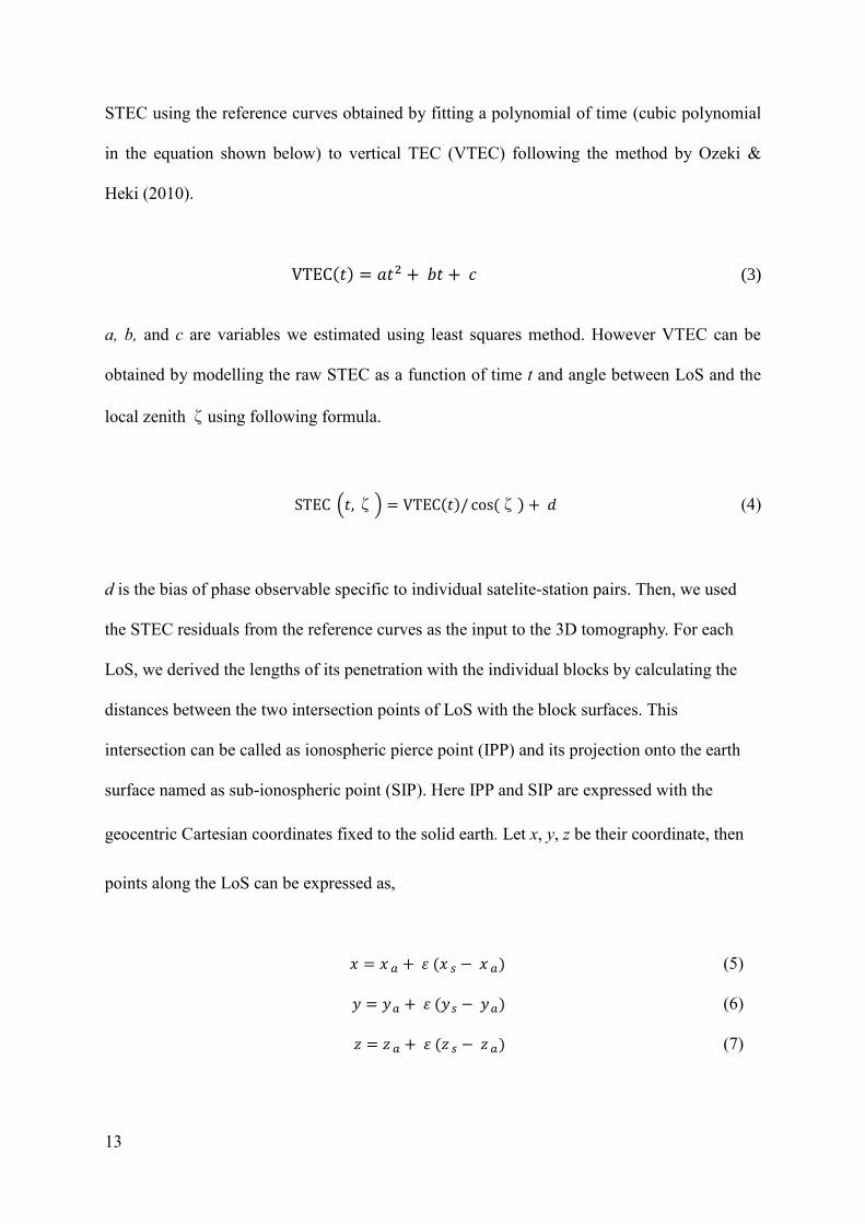
STEC using the reference curves obtained by fitting a polynomial of time (cubic polynomial

in the equation shown below) to vertical TEC (VTEC) following the method by Ozeki &

Heki (2010).

VTEC(𝑡) = 𝑎𝑡2 + 𝑏𝑡 + 𝑐 (3)

a, b, and c are variables we estimated using least squares method. However VTEC can be

obtained by modelling the raw STEC as a function of time t and angle between LoS and the

local zenith ζusing following formula.

STEC (𝑡,ζ) = VTEC(𝑡)/ cos(ζ) + 𝑑 (4)

d is the bias of phase observable specific to individual satelite-station pairs. Then, we used

the STEC residuals from the reference curves as the input to the 3D tomography. For each

LoS, we derived the lengths of its penetration with the individual blocks by calculating the

distances between the two intersection points of LoS with the block surfaces. This

intersection can be called as ionospheric pierce point (IPP) and its projection onto the earth

surface named as sub-ionospheric point (SIP). Here IPP and SIP are expressed with the

geocentric Cartesian coordinates fixed to the solid earth. Let x, y, z be their coordinate, then

points along the LoS can be expressed as,

𝑥 = 𝑥 𝑎 + 𝜀 (𝑥 𝑠 − 𝑥 𝑎) (5)

𝑦 = 𝑦 𝑎 + 𝜀 (𝑦 𝑠 − 𝑦 𝑎) (6)

𝑧 = 𝑧 𝑎 + 𝜀 (𝑧 𝑠 − 𝑧 𝑎) (7)

14

where xa, ya, za represent the receiver coordinate, xs, ys, zs represent the satellite coordinate.

The parameter, 𝜀, changes over a range from zero to one (0 < 𝜀 < 1), i.e. (x, y, z) signify the

receiver and satellite coordinates when is 0 and 1, respectively. Coordinates of points on the

up-down, east-west, and north-south surfaces of the block satisfy the following three

equations, respectively.

x2 + y2 + z2 = (R+H)2 (8)

y/x = tan 𝜑 (9)

z2/(x2+y2) = tan2 𝜃 (10)

There, R is the radius of the Earth, H, 𝜑, 𝜃 are the height, longitude and latitude of the

horizontal, vertical (north-south), vertical (east-west) surfaces of a block. The coordinates of

the LoS penetration points with these surfaces could be obtained by substituting x, y, z in (8)-

(10) with those in (5)-(7), and solving them for . After determining , we check the

penetration of LoS with blocks by examining the coordinates of the penetration points. Fig.

2.1 shows the geometry of LoS penetrating the blocks for Case 1 and 4.

By assuming electron density anomalies are uniform within individual blocks, the i-th

STEC anomaly yi can be modeled as the sum of the products of the electron density

anomalies of the j-th blocks Lj and the penetration lengths Aij, and the measurement error ei,

i.e.

𝑦𝑖 = ∑ 𝐴𝑖𝑗𝐿𝑗𝑗 + 𝑒𝑖 (11)

The set of equation (11) for all the LoS is written in a matrix form as

y = Ax + e (12)

where y is the vector composed of STEC anomalies yi, A is the Jacobian matrix composed of

Aij, x is the vector composed of unknown parameters xj (electron density anomalies of

15

individual blocks), and e is the errors. We estimated x by solving the normal equation

x = (AT A )-1 AT y (13)

after the Cholesky’s decomposition, i.e. by decomposing the normal matrix AT A into lower

triangular matrix L and its transpose.

AT A = L LT (14)

Although there are many LoS (Fig. 2.1), there are still blocks not penetrated by any

LoS. In this case, we need to regularize the normal matrix by certain numerical techniques.

Here, I applied the continuity constraint, i.e. we assume that neighboring blocks have the

same electron density anomalies with a certain allowance for the difference. Suppose block

number j is at the east side of block number i, then we assume xi and xj, the electron density

anomalies of these blocks, satisfy 𝑥𝑖 − 𝑥𝑗 = 0. One block normally has six neighboring

blocks (up, down, north, south, east, and south), and all these pairs are added to the normal

matrix as virtual observations (Nakagawa and Oyanagi, 1982). I did not constrain the block

pairs that are not juxtaposed.

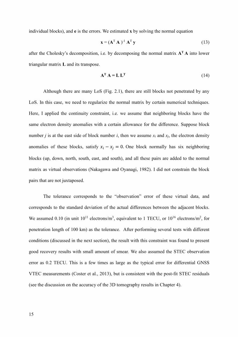
The tolerance corresponds to the “observation” error of these virtual data, and

corresponds to the standard deviation of the actual differences between the adjacent blocks.

We assumed 0.10 (in unit 1011 electrons/m3, equivalent to 1 TECU, or 1016 electrons/m2, for

penetration length of 100 km) as the tolerance. After performing several tests with different

conditions (discussed in the next section), the result with this constraint was found to present

good recovery results with small amount of smear. We also assumed the STEC observation

error as 0.2 TECU. This is a few times as large as the typical error for differential GNSS

VTEC measurements (Coster et al., 2013), but is consistent with the post-fit STEC residuals

(see the discussion on the accuracy of the 3D tomography results in Chapter 4).

16

Figure 2.1. Line-of-sight (LoS) distribution of the satellite-station pairs used for 3D

tomography for Case 1 above Kanto (a), and Case 4 above Kyushu (b).

17

Chapter 3

3.1. Resolution tests

A standard way to investigate the reliability of the 3D tomography solution is the

checkerboard resolution test. We assume Case 1, the Es patch over the Kanto District on 14

May 2010, and synthesized the LoS STEC anomaly data assuming the checkerboard-like

distributions of electron density anomalies with 0.60 and -0.60 TECU/100 km (Figure 3.1.)

and real satellite/station geometry at the time of Es appearance. We did not add artificial

noises to the synthetic data. Figure 3.2. shows the checkerboard-pattern distribution for Case

4, the Es patch over Kyushu District on 22 May 2010.

Figure 3.1. The 3D pattern of electron density anomalies used for the checkerboard

resolution test assuming Case 1 in the Kanto District. The result is given in Figure 3.3. We

gave alternating patterns of positive and negative anomalies as strong as ± 0.60 x

1011electrons/km3 (0.60 TECU/100 km) at low (a) and high (b) altitudes. We show the

vertical profiles at latitude 34.8 o (c) and 36.0 o (d), and longitude 138.6 o (e).

18

Figure 3.2. The 3D pattern of electron density anomalies for the checkerboard resolution test

assuming Case 4 in the Kyushu District, on 22 May 2010. We gave alternating patterns of

positive and negative anomalies as strong as ±0.60 x 1011 electrons/km3 at low (a) and high

(b) altitudes. We show the vertical profiles at latitude 30.5 o (c) and 32.0 o (d) and longitude

130.7 o (e).

Fig. 3.3. shows the distribution of the anomalies recovered using the synthetic data. It

suggests that we could well resolve structures as shown in Fig. 3.1. By comparing those two

map views, we see that the resolution at higher altitude (~255 km) is slightly poorer than that

in the lower height (~100 km). This reflects the better coverage (more penetration) of LoS for

lower blocks. They also suggest that the resolution is higher above land area and poorer

above the ocean. The result for Case 4 (Fig. 3.4.) is slightly worse, i.e. recovered blocks in

oceanic area show diagonal stripes, reflecting poor resolutions along the NE-SW axis.

Figure 3.3. Results of the checkerboard resolution test of the pattern shown in Figure 3.1. We

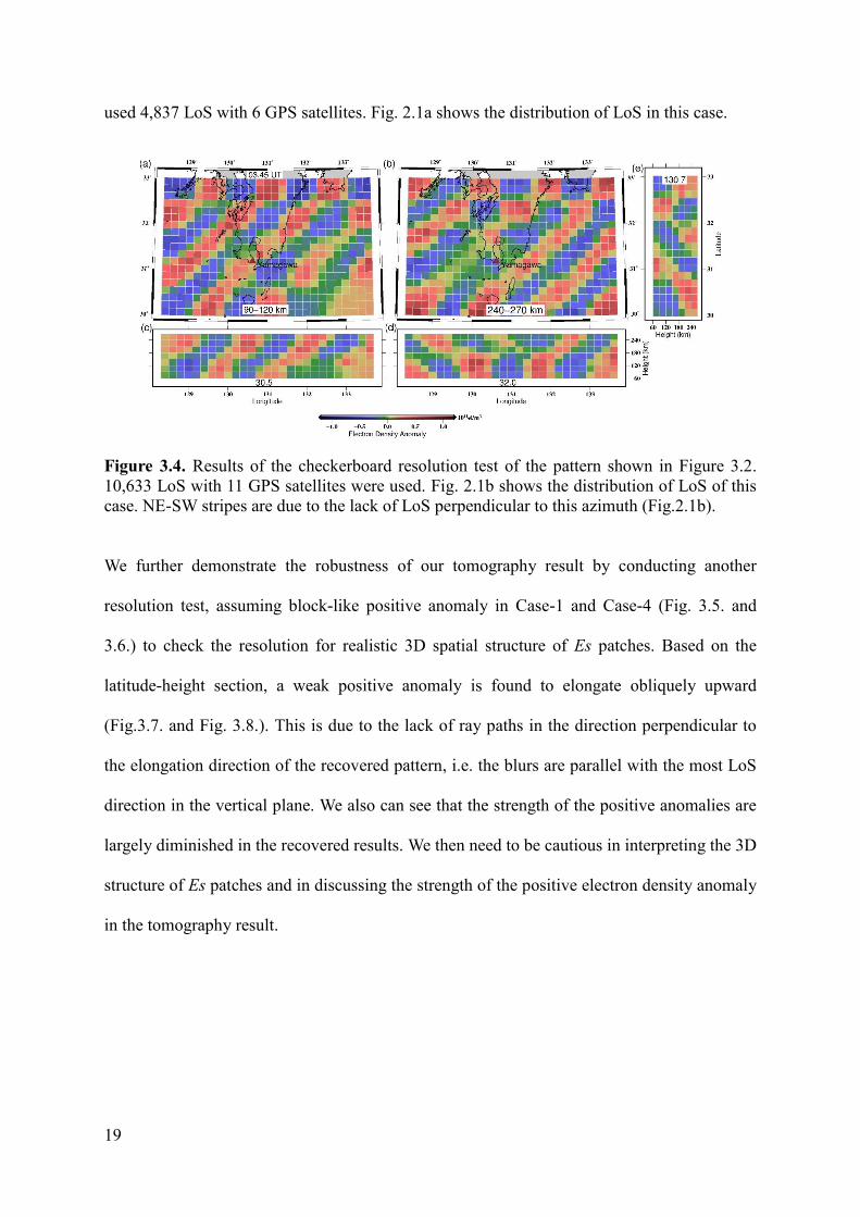
19

used 4,837 LoS with 6 GPS satellites. Fig. 2.1a shows the distribution of LoS in this case.

Figure 3.4. Results of the checkerboard resolution test of the pattern shown in Figure 3.2.

10,633 LoS with 11 GPS satellites were used. Fig. 2.1b shows the distribution of LoS of this

case. NE-SW stripes are due to the lack of LoS perpendicular to this azimuth (Fig.2.1b).

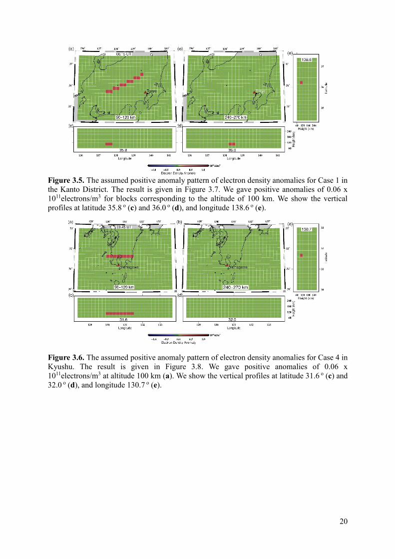
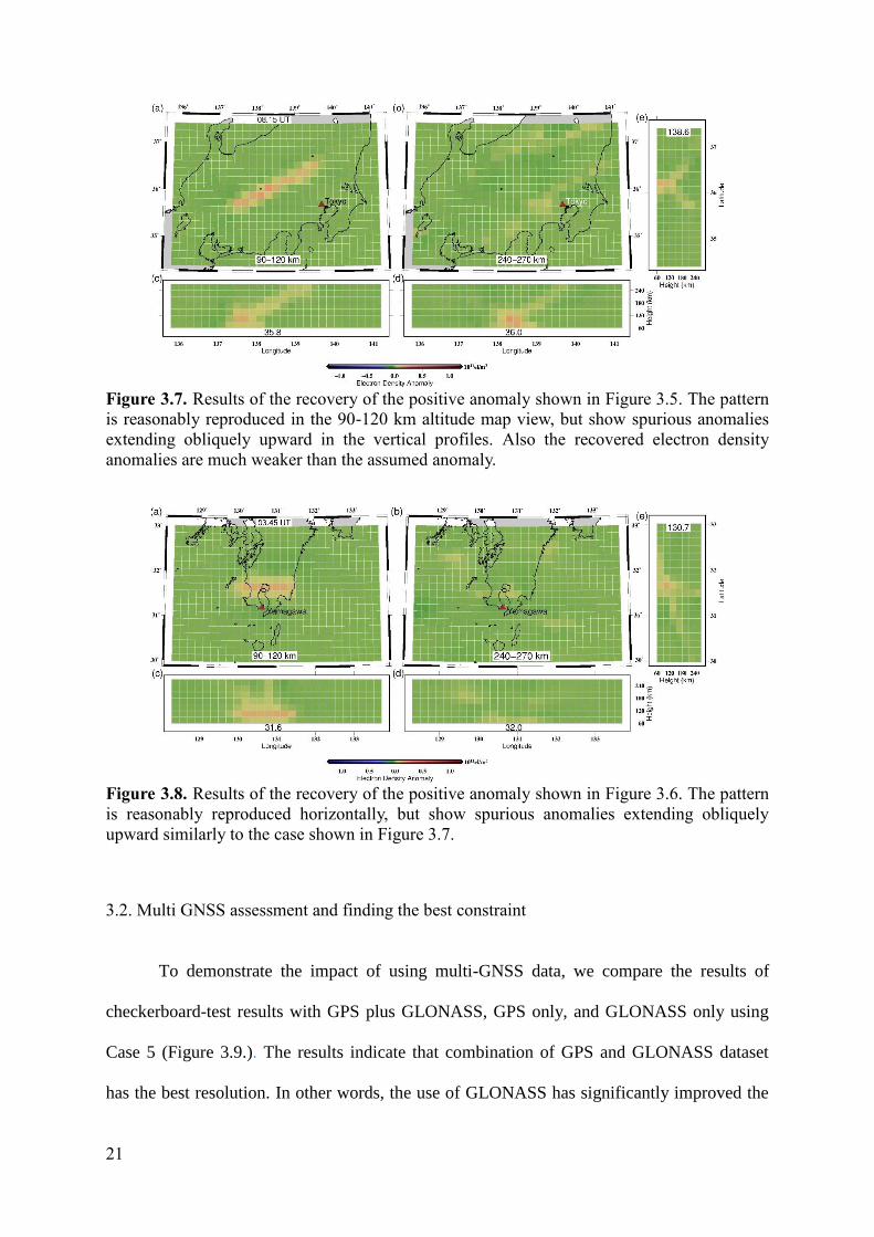
We further demonstrate the robustness of our tomography result by conducting another

resolution test, assuming block-like positive anomaly in Case-1 and Case-4 (Fig. 3.5. and

3.6.) to check the resolution for realistic 3D spatial structure of Es patches. Based on the

latitude-height section, a weak positive anomaly is found to elongate obliquely upward

(Fig.3.7. and Fig. 3.8.). This is due to the lack of ray paths in the direction perpendicular to

the elongation direction of the recovered pattern, i.e. the blurs are parallel with the most LoS

direction in the vertical plane. We also can see that the strength of the positive anomalies are

largely diminished in the recovered results. We then need to be cautious in interpreting the 3D

structure of Es patches and in discussing the strength of the positive electron density anomaly

in the tomography result.

20

Figure 3.5. The assumed positive anomaly pattern of electron density anomalies for Case 1 in

the Kanto District. The result is given in Figure 3.7. We gave positive anomalies of 0.06 x

1011electrons/m3 for blocks corresponding to the altitude of 100 km. We show the vertical

profiles at latitude 35.8 o (c) and 36.0 o (d), and longitude 138.6 o (e).

Figure 3.6. The assumed positive anomaly pattern of electron density anomalies for Case 4 in

Kyushu. The result is given in Figure 3.8. We gave positive anomalies of 0.06 x

1011electrons/m3 at altitude 100 km (a). We show the vertical profiles at latitude 31.6 o (c) and

32.0 o (d), and longitude 130.7 o (e).

21

Figure 3.7. Results of the recovery of the positive anomaly shown in Figure 3.5. The pattern

is reasonably reproduced in the 90-120 km altitude map view, but show spurious anomalies

extending obliquely upward in the vertical profiles. Also the recovered electron density

anomalies are much weaker than the assumed anomaly.

Figure 3.8. Results of the recovery of the positive anomaly shown in Figure 3.6. The pattern

is reasonably reproduced horizontally, but show spurious anomalies extending obliquely

upward similarly to the case shown in Figure 3.7.

3.2. Multi GNSS assessment and finding the best constraint

To demonstrate the impact of using multi-GNSS data, we compare the results of

checkerboard-test results with GPS plus GLONASS, GPS only, and GLONASS only using

Case 5 (Figure 3.9.). The results indicate that combination of GPS and GLONASS dataset

has the best resolution. In other words, the use of GLONASS has significantly improved the

22

accuracy of the result of the 3D tomography on land. However, diagonal patterns appearing

in the areas far from the land are not much improved.

Figure 3.9. Results of the checkerboard-test for Case 5 using both GPS and GLONASS data

(top), GPS data only (middle), and GLONASS data only (bottom). With only GLONASS, the

23

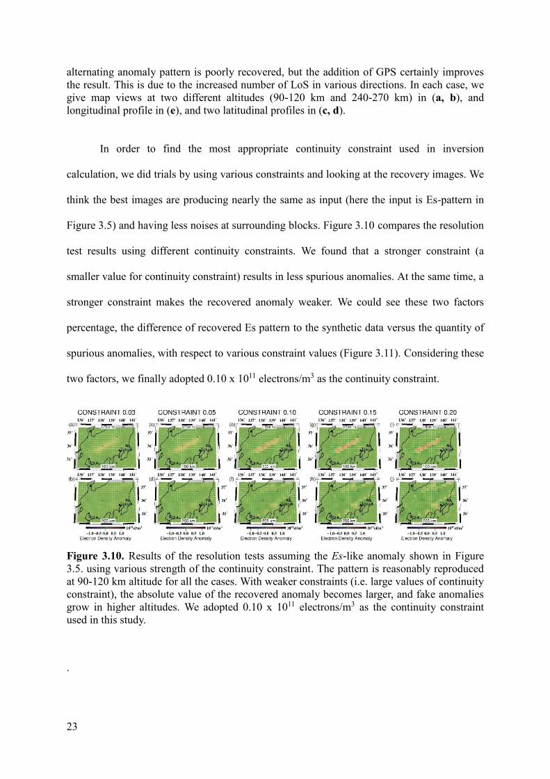
alternating anomaly pattern is poorly recovered, but the addition of GPS certainly improves

the result. This is due to the increased number of LoS in various directions. In each case, we

give map views at two different altitudes (90-120 km and 240-270 km) in (a, b), and

longitudinal profile in (e), and two latitudinal profiles in (c, d).

In order to find the most appropriate continuity constraint used in inversion

calculation, we did trials by using various constraints and looking at the recovery images. We

think the best images are producing nearly the same as input (here the input is Es-pattern in

Figure 3.5) and having less noises at surrounding blocks. Figure 3.10 compares the resolution

test results using different continuity constraints. We found that a stronger constraint (a

smaller value for continuity constraint) results in less spurious anomalies. At the same time, a

stronger constraint makes the recovered anomaly weaker. We could see these two factors

percentage, the difference of recovered Es pattern to the synthetic data versus the quantity of

spurious anomalies, with respect to various constraint values (Figure 3.11). Considering these

two factors, we finally adopted 0.10 x 1011 electrons/m3 as the continuity constraint.

Figure 3.10. Results of the resolution tests assuming the Es-like anomaly shown in Figure

3.5. using various strength of the continuity constraint. The pattern is reasonably reproduced

at 90-120 km altitude for all the cases. With weaker constraints (i.e. large values of continuity

constraint), the absolute value of the recovered anomaly becomes larger, and fake anomalies

grow in higher altitudes. We adopted 0.10 x 1011 electrons/m3 as the continuity constraint

used in this study.

.

24

Figure 3.11. The percentage of two factors, fake anomalies in a higher altitude (orange, right

y-axis) and difference of recovered Es pattern from the model (blue, left y-axis), used in

estimating the best value for the continuity constraint. I adopted 0.10 x 1011 electrons/m3

(TECU/100km) considering both factors, i.e. less fake anomalies and more consistency to the

assumed anomalies.

25

Chapter 4

4.1. Es 3D-Tomography result

In Figs. 4.1 and 4.2., we show results of 3D tomography for Case 1 and 4,

respectively. We performed the inversion at three time epochs (8:21, 8:23, 8:25 in Fig. 4.1.,

and 3:51, 3:53, 3:55 in Fig. 4.2.), and calculated their averages to reduce the random noise.

Considering the horizontal drift of these Es patches (Maeda and Heki, 2015), we think it is

not appropriate to increase the stacking period, i.e. the travel distance of Es patches may

exceed the block size for longer periods.

One of the purposes of this study is to justify the estimated heights of the Es

irregularities in previous studies (Maeda and Heki, 2014; 2015). The tomography results

shown in Figs. 4.1.a and 4.2.a clearly show that the high electron density anomalies mainly

reside in the 2nd layers from the bottom. Their height is 90-120 km, and corresponds to the E

region (unfortunately, 30 km is the height resolution of our 3D tomography, thus we cannot

discuss the Es patch thickness). At the same time, the positive anomalies do not appear in the

higher layers, e.g. at the F-region altitude of 180-210 km (Figure 4.1.b and 4.2.b). Es patches

are also recognized by latitudinal profiles (35.6 o N for the Kanto and 31.8 o N for the Kyushu

cases). These results are consistent with Maeda and Heki (2014) who inferred the Es lies at

height ~100 km. In Figs. 4.1.e and 4.2.e, we plotted time series of VTEC changes at stations

shown with black squares in Figs. 4.1.a and 4.2.a. We can see that the VTEC shows pulse-like

TEC enhancements when SIPs (sub-ionospheric point, assuming 100 km ionospheric height)

overlap with the Es patches recovered by 3D tomography.

26

Figure 4.1 a-d. Results of 3D tomography (average of the results at 8:21, 8:23, 8:25 UT) of

Case 1 Es patch that occurred on 14 May 2010 above the Kanto District, see Figure 4b of Maeda

and Heki (2014). We used 6 satellites and 4,828 LoS. Black curves in a describe the tracks

(moving northward) of the intersection of LoS with a thin layer at 90-120 km altitude (red

circles show the positions at 8:23 UT) for the station-satellite pairs shown in e. We show the

map views at altitudes 90-120 km (a) and 180-210 km (b), latitudinal profiles at 35.6 o N (c) and

35.9 o N (d). Black dashed lines in b indicate the latitudes for the profiles. Time series (red

curves) of VTEC residuals 7:50-9:00 UT from reference curves, observed at eleven GNSS

stations (black rectangle in a) with GPS satellite 29, show typical Es signatures as short-period

positive pulse around 8.5 UT (e).

Figure 4.2 a-d. Results of 3D tomography (average of 3:51, 3:53, 3:55 UT) of Case 4 Es patch

that occurred on 22 May 2010 above the Kyushu District, see Figure 1d of Maeda and Heki

(2015). We used 11 satellites and 10,547 LoS. Black curves in a describe the tracks (moving

southward) of the intersection of LoS with a thin layer at 90-120 km altitude (red circles show

the positions at 3:42 UT) for the station-satellite pairs shown in e. We show the map views at

altitudes 90-120 km (a) and 180-210 km (b), latitudinal profiles at 31.8 o N (c) and 32.0 o N (d).

Black dashed lines in b indicate the latitudes for the profiles. Time series (red curves) of vertical

TEC changes 2.5-4.5 UT, observed at ten stations (black rectangles in a), using GPS satellite 24

are shown in e. Clear Es signals are seen 3:30-3:45 UT as positive pulses.

27

4.2. Horizontal drift of Es patches and its vertical structure

We study the horizontal drift of Es patches by comparing the tomography results at

two time epochs separated by 15 minutes. Figs. 4.3 and 4.4. show the three cases in Kanto

(Cases 1-3) and two cases in Kyushu (Cases 4,5), respectively. In Case 1 and 2, the Es moves

southward, while in Case 3, 4, 5 they move northward, maintaining their altitude of ~100 km,

with speeds (30-100 m/s) consistent with the earlier report by Maeda and Heki (2015).

Figure 4.3. Horizontal drifts of three Es patches (Case 1: 14 May, 2010, Case 2: 21 May,

2010, and Case 3: 13 May 2012) above the Kanto District inferred by comparing the

snapshots at the first epoch (a, c, and e) and 15 minutes later (b, d, and f). At each epoch, we

show the map view (left) and the longitudinal profile (right). Black dashed lines indicate the

longitudes for the profiles.

28

Figure 4.4. Horizontal drifts of two Es patches (Case 4: 22 May 2010, and Case 5: 9 June

2013) above the Kyushu District inferred by comparing the snapshots at the first epoch (a, c)

and 15 minutes later (b, d). At each epoch, we show the map view (left) and the longitudinal

profile (right). Black dashed lines indicate the longitudes for the profiles.

In the longitudinal profiles of the results (Figures 4.3., 4.4.), we often see faint

positive anomalies continue obliquely upward from their Es irregularities at ~100 km

altitude. One might think that they represent real plasma density anomaly structure extending

from the main bodies of Es. However, similar pattern also appears in the resolution test

results with the Es-like structures (Figs. 3.7 and 3.8.), which suggests that they are artifacts

due to the lack of data with LoS perpendicular to the direction of the fake structure

elongation.

4.3. Accuracy of tomography result

In order to assess our tomography accuracy result, we show two quantities. First we

show formal errors, i.e. the square-root of the diagonal components of the covariance matrix,

the inverse of the normal matrix. It gives the idea about the non-uniform distribution of the

accuracy of the tomography results. Figures 4.5., 4.6. show relatively high accuracy for

29

blocks at lower altitude (90-120 km) above land, and lower accuracy for high altitude blocks

(240-270 km) over the ocean. This is consistent with the results of the classical checkerboard

test discussed earlier (Figs. 3.3, 3.4.). Secondly we compare the distributions of post-fit

residuals of STEC (Figures 4.7. bottom panels) with the raw observations (Figures 4.7. upper

panels). In each case, the post-fit residual show much smaller dispersion, and its standard

deviation is similar to the assumed STEC observation errors (0.2 TECU).

Figure 4.5. Formal error distribution of the 3D tomography result of Case 1 (14 May 2010)

for boxes at altitude 90-120 km (a) and 240-270 km (b). We also show the latitudinal profiles

at 35.6 o (c) and 35.0 o (d) and longitudinal profile at 138.6 o (e). They are obtained as square-

root of the diagonal components of the inverse of the normal matrix. We can see the errors

are uniform in most of the region, with degradation in the top layer and along the rim.

30

Figure 4.6 Formal error distribution of tomography result for Case 4 (22 May 2010) for

boxes at altitude 90-120 km (a) and 240-270 km (b). We also show the latitudinal profiles at

31.5 o (c) and 32.0 o (d) and longitudinal profile at 130.7 o (e). We can see that errors are

significantly larger above ocean.

Figure 4.7 The distribution of the input STEC anomalies (orange) and post-fit residuals

(blue) for Cases 1-5. The residuals become smaller than the observations, suggesting that the

tomography results reasonably reproduced the observations.

31

Chapter 5

5.1. Conclusions

We studied five cases of daytime mid-latitude Es irregularities with the 3D

tomography technique using STEC residual data from GEONET GNSS stations. We

estimated the electron density anomalies in the boxes set up in a 3D space above the Kanto

and the Kyushu districts by using linear least-squares inversion technique stabilizing the

solution by introducing continuity constraints. We also confirmed the performance of our

tomography result by two kinds of resolution test, i.e. the classical checkerboard test and the

other test assuming Es-like structures.

By performing the 3D tomography for the five cases of Es appearances selected from

earlier studies (Maeda and Heki, 2014; 2015), we confirmed that the Es patches lie at altitude

~100 km. We also confirmed the earlier reports that Es patches show frontal shape elongated

in E-W and drift horizontally with the speed consistent with Maeda and Heki (2015). We

found faint positive anomalies extending obliquely upward from the main body of Es, but we

confirmed that they are artifacts caused by lack of LoS perpendicular to the fake 3D structure.

32

References

Austen J R, Franke J, Liu C H (1988) Ionospheric imaging using computerized tomography.

Radio Sci. 23: 299–307.

Bernhardt P A, Selcher C A, Siefring C, Wilkens M, Compton C, Bust G, Yamamoto M,

Fukao S, Ono T, Wakabayashi M, Mori H (2005) Radio Tomographic Imaging of

Sporadic-E layers during SEEK-2. Ann. Geophys., 23:2357–2368.

Cahyadi M N , Heki K (2013) Ionospheric disturbances of the 2007 Bengkulu and the 2005

Nias earthquakes, Sumatra, observed with a regional GPS network. J. Geophys. Res. Sp.

Phys. 118, 1777–1787. doi:10.1002/jgra.50208

Chen C H, Saito A, Lin C H, Yamamoto M, Suzuki S, Seemala G K (2016) Medium‑ scale

traveling ionospheric disturbances by three‑dimensional ionospheric GPS tomography.

Earth, Planets Space, 68:32. doi:10.1186/s40623-016-0412-6.

Coster A, Williams J, Weatherwax A, Rideout W, Herne D (2013) Accuracy of GPS total

electron content: GPS receiver bias temperature dependence. Radio Sci. 48: 190–196.

doi:10.1002/rds.20011.

Dautermann T, Calais E, Lognonne P, Mattioli G S (2009a) Lithosphereatmosphere-

ionosphere coupling after 2003 explosive eruption of the Soufriere Hills Volcano,

Montserrat. Gephysical Journal International 179: 1527-1546.

Garcia-Fernandez M, Tsuda T (2006) A global distribution of sporadic E events revealed by

means of CHAMP-GPS occultations. Earth Planets Space 58: 33–36.

Heki K (2006) Explosion energy of the 2004 eruption of the Asama Volcano, central Japan,

inferred from ionospheric disturbances. Geophysical Research Letters 33: L14303,

http://dx.doi.org./10.1029/2006GL026249.

Jayachandran P T, Ram P S, Rao P V S R, Somayajulu V V (1999) Sequential sporadic-E

layers at low latitudes in the Indian sector. Ann. Geophy., 17:519–525.

33

Kirkwood S, Nilsson H (2000) High-latitude sporadic-e and other thin layers – the role of

magnetospheric electric fields. Space Sci. Rev. 91:579–613.

Kurihara J, Kurihara Y K, Iwagami N, Suzuki T, Kumamoto A, Ono T, Nakamura M, Ishii M,

Matsuoka A, Ishisaka K, Abe T, Nozawa S (2010) Horizontal structure of sporadic E

layer observed with a rocket ‐ borne magnesium ion imager. J. Geophys. Res. 115: 2–7.

doi:10.1029/2009JA014926.

Maeda J, Heki K (2015) Morphology and dynamics of daytime mid-latitude sporadic-E

patches revealed by GPS total electron content observations in Japan. Earth Planets

Space 67(1): 89. doi:10.1186/s40623-015-0257-4.

Maeda J, Heki K (2014) Two-dimensional observations of midlatitude sporadic e

irregularities with a dense GPS array in Japan. Radio Sci. 49(1): 28–35.

doi:10.1002/2013RS005295.

Maeda J, Suzuki T, Furuya M, Heki K (2016) Imaging the midlatitude sporadic E plasma

patches with a coordinated observation of spaceborne InSAR and GPS total electron

content. Geophys. Res. Lett, 43:1419–1425. doi:10.1002/2015GL067585.

Nakagawa T, Oyanagi Y (1982) Observation data analysis with the least-squares method, UP

Applied Mathematics Series Vol.7, Tokyo University Press, pp. 216. (in Japanese)

Nakashima Y, Heki K (2014) Ionospheric hole made by the 2012 North Korean rocket

observed with a dense GNSS array in Japan. Radio Sci. 49, 497–505.

doi:10.1002/2014RS005413

Ozeki M, Heki K (2010) Ionospheric holes made by ballistic missiles from North Korea

detected with a Japanese dense GPS array. J. Geophys. Res. 115, 1–11.

doi:10.1029/2010JA015531.

Resende L C A, Denardini C M (2012) Equatorial sporadic E -layer abnormal density

enhancement during the recovery phase of the December 2006 magnetic storm : A case

34

study, Earth Planets Space, 64: 345–351. doi:10.5047/eps.2011.10.007.

Seemala G K, Yamamoto M, Saito A, Chen C H (2014) Three-dimensional GPS ionospheric

tomography over Japan using constrained least squares. J. Geophys., Res. Space

Physics, 119:3044-3052. doi:10.1002/2013JA019582.

Saito S, Suzuki S, Yamamoto M, Chen C H, Saito A (2016) Real-time Ionosphere Monitoring

by Three-dimensional Tomography Over Japan. Proc. 29th Int. Tech. Meeting, Satellite

Division of the Institute of Navigation (ION GNSS+ 2016), Portland, Oregon. pp:706-

713.

Tang J, Yao Y, Zhang L, Kong J (2015) Tomographic reconstruction of ionospheric electron

density during the storm of 5-6 August 2011 using multi-source data. Nat. Publ. Gr. 1–

11. doi:10.1038/srep13042

Yamamoto M, Ono T, Oya H, Tsunoda R T, Larsen M F, Fukao S, Yamamoto M (1998)

Structures in sporadic-E observed with an impedance probe During the SEEK campaign:

Comparisons with neutral-wind and radar-echo observations, Geophys. Res. Lett, 25:

1781–1784.

Wakabayashi M, Ono T, Mori H, Bernhardt P A (2005) Electron density and plasma waves in

mid-latitude sporadic-E layer observed during the SEEK-2 campaign, Ann. Geophys.,

23:2335–2345.

Whitehead J D (1970) Production and Prediction of Sporadic E. Rev. Geophys. Space Phys.

8:65-144.

Yokoyama T, Yamamoto M, Fukao S, Takahashi T, Tanaka M (2005) Numerical simulation of

mid-latitude ionospheric E-region based on SEEK and SEEK-2 observations, Ann.

Geophys., 23:2377–2384.