3D SOFTWARE SIMULATIONS COMPARED WITH EXPERIMENTAL DATA FOR THE

INTERFERENCE BETWEEN A CATHODICALLY PROTECTED UNDERGROUND STORAGE TANK

(UST) AND A CONCRETE FOUNDATION

B. Van den Bossche, M. Purcar, L. Bortels, A. Dorochenko Elsyca N.V.

Kranenberg 6, 1731 Zellik Belgium

J. Deconinck Vrije Universiteit Brussel

Department IR\ETEC Pleinlaan 2, 1050 Brussels

Belgium

ABSTRACT

This paper presents a 3D software tool for the design and optimization of cathodic protection systems

for buried and submerged structures. It provides the corrosion engineer an intelligent tool for managing

operational costs, significantly reducing expensive commissioning surveys and costly repairs, adding

major value to the cathodic protection business.

In this paper, simulations are compared to experimental data obtained by the Nederlandse Gasunie.

The case that has been investigated is the interference between a cathodically protected underground

storage tank (UST) and a concrete foundation. Experiments show that the protection level at the side of

the UST near the concrete foundation is only –600 to –700 mV versus CSE, while the far field potential

is about -1200 mV. The interference can be mitigated by putting a PVC screen between the UST and

the concrete fundation. This increases the protection level on the tank with about -200 mV at the

foundation side, while the potential at the other side of the tank is hardly affected. The agreement

between the experimental data obtained on site and numerical simulations, using a two-layer model

that accounts for the ground water level, is very good.

Keywords: cathodic protection simulations, advanced software package, multi-layer model

INTRODUCTION

Cathodic Protection (CP) systems are widely applied to buried tank and pipeline structures, as they

compensate (by electrochemical means) for the loss in physical protection due to the degradation of

tank coatings over time. Most often, these CP systems contain a series of impressed current anode

ground beds (though sacrificial anodes can also be used), placed at a remote distance from the pipes

and tanks. The entire configuration of the CP system and the buried structures has particular

characteristics that necessitate and justify the use of numerical simulations.

First, the hidden character and low accessibility of these structures make installation, maintenance and

repair very expensive. Also, the geometry of most steel structures that are subject to cathodic

protection is too complex to allow analytical or even empirical estimations for the determination of the

local protection level.

Numerical modeling provides significant relieve by pointing out insufficiently protected regions -

possibly subject to corrosion, and overprotected regions - subject to hydrogen evolution and hence

coating delamination or hydrogen embrittlement. As a consequence, numerical modeling allows

simplification and optimization of installation, maintenance and repair. Moreover, models provide

reference values for measurements on operational sites, enabling the user to trace and solve any

possible anomaly.

Most of the publications dealing with the computation of the CP of buried or submerged structures are

based on the well known Boundary Element Method (BEM) [1]. Orazem et al. [2,3] use a 3D BEM

approach to compute the protection level of large coating defects on pipelines. Results are presented

for a pipe segment of limited length (10 feet), in presence of a parallel anode system. Riemer and

Orazem [4] produced results for a longer pipeline (> 6 km) with coating defects of varying size and

investigated the ability of coupons in the vicinity of the defects to measure off-potentials. Adey [5]

applied a full 3D approach to calculate the potential field in the neighborhood of jacket joints under

cathodic protection of sacrificial anodes. The present authors [6] used a 3D coupled multi-domain BEM

approach to simulate the protection level of a buried pipe segment surrounded by a concrete vault.

The simulations presented in this paper are obtained using a software package [7] with fundamentals

as decribed in the next section.

MATHEMATICAL MODEL

The software is entirely CAD integrated offering a user-friendly interface for the CP design, including file

import from numerous other CAD packages. The mathematical model is based on the potential model

and includes the key features listed below:

• Parameterisation of all geometrical dimensions

• Simulation of 3D CP-configurations with arbitrary complexity

• Interference from 3rd party CP-systems

• Ohmic drop effects in the soil or water

• Anodic and cathodic reaction polarization behavior

• Impressed current and sacrificial ground beds / anodes

• Floating (not contacted) electrodes (for example casings)

• Multi-layered soils with varying resistivity

• Local metal dissolution calculation based on Faraday’s law.

The resulting non-linear system equations are solved using a Newton-Raphson iterative method [8],

combined with an advanced linear solver to solve the linear system of equations that appears during

each iteration in the Newton-Raphson procedure. An automated hybrid grid generator is used to

produce the high quality meshes that are required for the computations [9]. Full details can be found in

reference [6].

DESCRIPTION OF THE PROBLEM

The configuration of interest consists of a buried tank with concrete foundation (the latter assumed to

be non-conducting) and part of steel reinforced concrete foundation of a neighbouring building (Figure

1). The foundation is electrically connected to the CP system, hence exhibits a negative impact on the

protection level of the tank surface. An insulating screen is installed between the tank and the

foundation in order to limit the impact of the concrete foundation.

FIGURE 1 - configuration of tank, foundation, screen and surrounding computational domain

(front and back side not shown - dimensions in mm)

The tank has a diameter of 1.3 m, 4 m length and is positioned about 0.9 m below the earth surface

(Figure 2). For computational purposes, a sufficiently large box has been defined that surrounds the

configuration of interest, the top plane coinciding with the earth surface and the side wall opposite to

the tank being identified with the far field. Also a series of small cubes has been defined, representing

possible positions of the reference electrode in perforated probe tubes. These small cubes are

considered insulating, hence do not affect the current density distribution in the soil, they simply take

the potential of the surrounding soil.

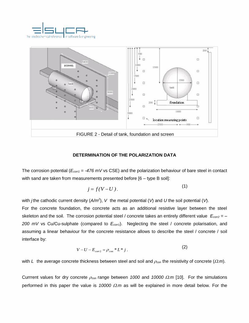
FIGURE 2 - Detail of tank, foundation and screen

DETERMINATION OF THE POLARIZATION DATA

The corrosion potential (Ecorr1 = -476 mV vs CSE) and the polarization behaviour of bare steel in contact

with sand are taken from measurements presented before [6 – type B soil]:

)UV(fj . (1)

with j the cathodic current density (A/m2), V the metal potential (V) and U the soil potential (V).

For the concrete foundation, the concrete acts as an additional resistive layer between the steel

skeleton and the soil. The corrosion potential steel / concrete takes an entirely different value Ecorr2 = –

200 mV vs Cu/Cu-sulphate (compared to Ecorr1). Neglecting the steel / concrete polarisation, and

assuming a linear behaviour for the concrete resistance allows to describe the steel / concrete / soil

interface by:

jLEUV concorr **2 . (2)

with L the average concrete thickness between steel and soil and con the resistivity of concrete (.m).

Currrent values for dry concrete con range between 1000 and 10000 .m [10]. For the simulations

performed in this paper the value is 10000 .m as will be explained in more detail below. For the

coated tank, it is assumed that the resistance of the coating is in series with the polarization resistance

of the system steel/sand:

)*( jLUVfj coat . (3)

The value of L coat is not known a priori. It can be calculated from the fact that a current density j of -

5.0E-6 A/m2 is needed [10] to obtain a minimum protection level V-U of –850 mV vs CSE. As a result a

value of L coat = 80.000 . m2 is obtained. The curve presented by equation (3) exhibits a linear

behaviour due to the high value for the coating resistance.

RESULTS

Model with uniform resistivity

The computational domain surrounding the tank and foundation is taken big enough in order to ensure

that the side walls and bottom can be considered as ”far field”. The far field potential has been taken

from measurements [11] and yields 1984 mV (average of two measurements (2011 and 1958 mV).

The measured soil resistivity [11] is 780 .m (average value at different depths). The values for the

resisitivity and characteristic thickness of the concrete around the rebar are tuned based on comparison

between measured and simulated tank-to-soil potentials at the earth surface (situation with screen).

Measured values for the tank-to-soil potentials [11] are about -700 mV (vs CSE) for the foundation side

of the tank and about -1200 mV (vs CSE) for the far field side, as measured with respect to the

perforated measurement tubes. This results in the following values: con = 10000 .m and L = 10 cm.

Results are presented in Figure 3 for one of the trajectories which data have been measured. The

distance between the concrete foundation (left) and the far field (right) is 30 m.

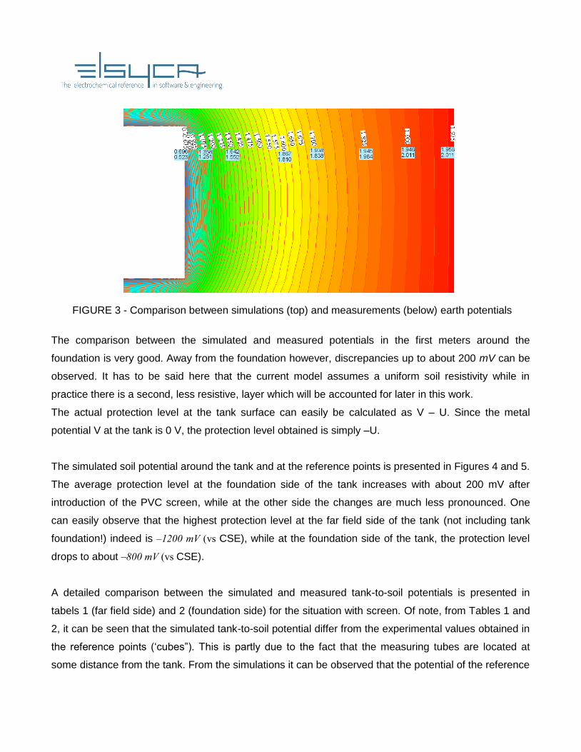
FIGURE 3 - Comparison between simulations (top) and measurements (below) earth potentials

The comparison between the simulated and measured potentials in the first meters around the

foundation is very good. Away from the foundation however, discrepancies up to about 200 mV can be

observed. It has to be said here that the current model assumes a uniform soil resistivity while in

practice there is a second, less resistive, layer which will be accounted for later in this work.

The actual protection level at the tank surface can easily be calculated as V – U. Since the metal

potential V at the tank is 0 V, the protection level obtained is simply –U.

The simulated soil potential around the tank and at the reference points is presented in Figures 4 and 5.

The average protection level at the foundation side of the tank increases with about 200 mV after

introduction of the PVC screen, while at the other side the changes are much less pronounced. One

can easily observe that the highest protection level at the far field side of the tank (not including tank

foundation!) indeed is –1200 mV (vs CSE), while at the foundation side of the tank, the protection level

drops to about –800 mV (vs CSE).

A detailed comparison between the simulated and measured tank-to-soil potentials is presented in

tabels 1 (far field side) and 2 (foundation side) for the situation with screen. Of note, from Tables 1 and

2, it can be seen that the simulated tank-to-soil potential differ from the experimental values obtained in

the reference points (‘cubes”). This is partly due to the fact that the measuring tubes are located at

some distance from the tank. From the simulations it can be observed that the potential of the reference

points differs about 100 mV from the actual soil potential near the tank. This means that the measured

value at the far field of the tank are too optimistic while at the other side of the tank, the values are too

pessimistic.

FIGURE 4 - Soil potential (V) around tank (situation without screen)

FIGURE 5 - Soil potential (V) around tank (situation with screen).

TABLE 1

Tank-to-soil potential (mV vs CSE) at the far field side (single layer model) for all reference

locations. Measured values in black (left) – simulated values in red (right)

Depth [mm] Left Middle Right

-500 -1289 -1285 -1277

-1000 -1474 -1295 -1489 -1291 -1500 -1288

-1500 -1484 -1303 -1493 -1300 -1505 -1297

-2000 -1492 -1309 -1500 -1309 -1515 -1307

-2500 -1510 -1318 -1519 -1315 -1535 -1312

-3000 -1515 -1328 -1529 -1322 -1540 -1319

TABLE 2

Tank-to-soil potential (mV vs CSE) at the foundation side (single layer model) for all reference

locations. Measured values in black (left) – simulated values in red (right)

Depth [mm] Left Middle Right

-500 -1059 -1059 -1056

-1000 -1228 -1083 -1202 -1084 -1177 -1079

-1500 -1255 -1101 -1228 -1103 -1208 -1100

-2000 -1276 -1125 -1253 -1126 -1244 -1124

-2500 -1310 -1146 -1298 -1156 -1280 -1152

-3000 -1324 -1163 -1305 -1165 -1290 -1161

Two-layer model

In the previous section it has been observed that the simulated potential at the earth surface at larger

distances from the foundation differed +/- 200 mV from the measured data (see Figure 3). This

discrepancy in results is due to the fact that the soil resistivity has been assumed to be uniform.

In this section, a two-layer model will be introduced. The top layer has a uniform soil resistivity with the

same value as before (i.e. 780 m). The thickness and resistivity of the second, less resistive layer

(accounting for the ground water), will be tuned in order to match the measured potential values at the

earth surface with the simulations. The resistivity of the second layer can be used to fine-tune the

potential near the concrete foundation while the starting depth of the ground water level allows to fit the

potentials at larger distances.

From this it turns out that a resistivity value for the second layer of about 150 m, starting from a depth

of about 5 m, yields a very good agreement between the measured and simulated earth potentials over

the complete trajectory (30 m in length).

0

0.5

1

1.5

2

2.5

0 5 10 15 20 25 30 35

afstand tot betonnen fundering / m

bo

dem

po

ten

tia

al la

ng

s m

aa

ivel

d / V

Figure 6 - Earth potential (in V) as a function of distance (in m) to foundation. Measured values

(), single layer model simulations with = 780 m (bottom curve), double layer

model simulations with = 780 m/150 m (top curve)

A detailed comparison between the simulated and measured tank-to-soil potentials for the two layer

model is presented in tabel 3 (far field side) and 4 (foundation side) for the situation with screen. It can

be seen that the agreement between both values is very good for the first 1.5 m while for the reference

points at deeper locations the discrepancy is a little higher. This suggests that it is close to the optimal

combination for the start point and resistivity of the second layer.

Distance to foundation [m]

Ea

rth

pote

ntia

l [V

]

TABLE 3

Tank-to-soil potential (mV vs CSE) at the far field side (two layer model)

for all reference locations. Measured values in black (left) – simulated values in red (right).

Depth [mm] Left Middle Right

-500 -1509 -1506 -1506

-1000 -1474 -1523 -1489 -1522 -1500 -1520

-1500 -1484 -1539 -1493 -1540 -1505 -1539

-2000 -1492 -1561 -1500 -1563 -1515 -1560

-2500 -1510 -1582 -1519 -1584 -1535 -1584

-3000 -1515 -1600 -1529 -1606 -1540 -1606

TABLE 4

Tank-to-soil potential (mV vs CSE) at the foundation side (two layer model)

for all reference locations. Measured values in black (left) – simulated values in red (right).

Depth [mm] Left Middle Right

-500 -1193 -1203 -1197

-1000 -1228 -1239 -1202 -1254 -1177 -1251

-1500 -1255 -1285 -1228 -1302 -1208 -1299

-2000 -1276 -1333 -1253 -1352 -1244 -1352

-2500 -1310 -1392 -1298 -1422 -1280 -1422

-3000 -1324 -1438 -1305 -1455 -1290 -1456

CONCLUSIONS

In this paper a 3D software tool for the design and optimisation of cathodic protection systems for

buried and submerged structures has been presented. The integration of the package in a professional

CAD environment, allows the user to optimize the cathodic protection configuration (e.g. size and

location of PVC screen, anode location) in a fast and flexible manner.

Using the software package, the interference between a cathodically protected underground storage

tank (UST) and a concrete foundation has been investigated. The resistivity of the concrete has been

tuned such that the measured and simulated ground level potentials match. A first set of simulations,

based on a uniform soil resistivity, predicts that the presence of a PVC screen between tank and

foundation increases the protection level of the tank at the foundation side with about 150 to 200 mV.

The measured and simulated values show a discrepancy of about 150 mV which already manifests

itself in the far field region. This suggests the presence of a multi-layer soil with varying resistivity,

coupled with the ground water level.

A second set of simulations based on a two layer model, with the second layer being much less

resistive, shows very good agreement between the measured and simulated earth level potentials.

Comparison between measured and simulated tank potentials suggests that the chosen values are

close to the optimal combination for the start point and resistivity of the second layer.

ACKNOWLEDGEMENTS

The authors wish to thank Ir. Pieter Stehouwer, Ir. Ing. Arie Dam and Ir. Kees Dijkstra, Nederlandse

Gasunie, Groningen, Nederland for their excellent help in providing and discussing the experimental

data.

REFERENCES

1. C.A. Brebbia, Boundary Element Techniques – Theory and Applications in Engineering, Springer-

Verlag Berlin, Heidelberg, 1983.

2. M.E. Orazem, J.M. Esteban, K.J. Kennelley, R.M. Degerstedt, Corrosion 53 (1997) 427.

3. M.E. Orazem, J.M. Esteban, K.J. Kennelley, R.M. Degerstedt, Corrosion 53 (1997) 264.

4. D.P. Riemer, and M.E. Orazem, Corrosion 56(2000)794.

5. R.A. Adey, Topics in Boundary Element Research, vol. 7, Electrical Engineering Applications,

chapter 3, Springer-Verlag Berlin, Heidelberg 1990.

6. M. Purcar, B. Van den Bossche, L. Bortels, J. Deconinck, P.Wesselius, Corrosion 59 (2003)

1019.

7. Elsyca CPMasterV1.0, User Manual, www.elsyca.com.

8. J. Deconinck, Current distributions and Electrode Shape Changes in Electrochemical Systems,

Lecture Notes in Engineering 75, Springer Verlag Berlin, ISBN 3-540-55104-2, 1992.

9. Athanasiadis A.N., Deconinck H., Int. J. Numer. Meth. Eng. 58 (2003) 301

10. Gasunie, OSB Voortgangsrapportage-001 (Internal Report), 30 January 2004.

11. Hommema, (Internal Report), 27 May 2005.