3d shape analysis: construction, classification and matching
TRANSCRIPT

3D SHAPE ANALYSIS: CONSTRUCTION, CLASSIFICATION ANDMATCHING
DISSERTATION FOR THE DEGREE OF
DOCTOR OF PHILOSOPHY IN SYSTEM ENGINEERING
SHAOJUN LIU
OAKLAND UNIVERSITY
2007

3D SHAPE ANALYSIS: CONSTRUCTION, CLASSIFICATION AND MATCHING
by
SHAOJUN LIU
A dissertation submitted in partial fulfillment of therequirements for the degree of
DOCTOR OF PHILOSOPHY IN SYSTEM ENGINEERING
2007
Oakland UniversityRochester, Michigan
APPROVED BY:
Jia Li, Ph.D., Chair Date
Ishwar K. Sethi, Ph.D. Date
Laszlo Liptak, Ph.D. Date
Andrzej Rusek, Ph.D. Date

c© Copyright by SHAOJUN LIU, 2007All rights reserved
ii

To My Father and Mother
iii

ACKNOWLEDGMENTS
Here I would like to thank my advisor Dr. Jia Li for her support and guidence
throughout my Ph.D. research. Starting from research ABC, she lead me into this
challenging area of 3D shape analysis. As an active researcher herself, she pointed me
to promising directions and we frequently discussed various problems together. I
benefit enormously from her insight and rich knowledge in this area. She is also a
friend in life. Her kind support enables me to devote myself to research
whole-heartly. Without the favorable environment she created, it would be
impossible for me to do Ph.D. research.
I sincerely thank my Ph.D. advisory committee members, Dr. Ishwar K.
Sethi, Dr. Laszlo Liptak, and Dr. Andrzej Rusek. Their insightful suggestions and
teaching helped me to accomplish this Ph.D. research. Special thanks to Dr. Sethi
for inviting me to his lab meetings and introducing me into a summer project on
fetal imaging in Beaumont hospital.
I am grateful to Dr. Wesley Lee, Dr. Russel Deter and Ms. Beverley Mc Nie
for their support on the fetal imaging project. I wish to express my gratitude to Dr.
Mingkun Li, Dr. Jun Tan and Dingguo Chen for their help on pattern recognition
techniques, and REU students Bryan Bonvallet and Nikolla Griffins for their
enlightening discussions on 4D hyperspherical harmonics. I appreciate my colleague
Weihong Niu for assisting me with lab environments, and Chiayang Hung in
programming issues.
Last I thank my parents and my dear wife for their love, support and
sacrifices on my Ph.D. research.
SHAOJUN LIU
iv

ABSTRACT
3D SHAPE ANALYSIS: CONSTRUCTION, CLASSIFICATION AND MATCHING
SHAOJUN LIU
Chair: Jia Li, Ph.D.
Surface construction is a widely studied topic in computer graphics and vi-
sion. Polygonal meshes generated by surface construction process are extensively
used in various graphic areas, such as scene rendering and texture mapping. March-
ing Cubes (MC) method is the most popular method in surface construction. Exist-
ing MC methods require sample values at cell vertices to be non-zero after thresh-
olding or modify them otherwise. The modification may introduce problems to a
constructed surface, such as topological changes, representation error, and preference
to positive or negative values. This dissertation presents a generalized MC algorithm
for surface construction. It constructs surface patches by exploring cycles in cells
without changing sample values at vertices, thus allows cell vertices with zero sam-
ple values to lie on the constructed surface. The simulation results show that the
proposed Zero-Crossing MC (ZMC) method better preserves topologies of implicit
surfaces that pass through cell vertices and represents the surfaces more accurately.
Its efficiency is comparable to existing MC methods in constructing surfaces.
As available 3D models on the Internet increase dramatically, efficiently search-
ing relevant shape models is requested by many applications such as computer ani-
mation, computer aided design (CAD) and protein matching. Shape-based retrieval
of 3D data has been an active research area in disciplines such as computer vision,
mechanical engineering and chemistry. The performance of 3D shape search engine,
however, is far behind that of text, such as Google search engine. A new method for
v

three dimensional (3D) genus-zero shape classification is proposed. It conformally
maps a 3D mesh onto a unit sphere and uses normal vectors to generate a spherical
normal image (SNI). Unlike Extended Gaussian Image (EGI) which has an ambigu-
ity problem, SNI is unique for each shape. Spherical harmonics coefficients of SNIs
are used as feature vectors and self-organizing map is adopted to explore the struc-
ture of a shape model database. Since the method compares only SNIs of different
objects, it is computationally more efficient than methods that compare multiple
2D views of 3D objects. The experimental results show that the proposed method
can discriminate collected 3D shapes very well, and is robust to mesh resolution and
pose difference.
For general shape classification and matching, rotation invariant methods
based on concentric spheres model (CSM) cut 3D objects along radii. As a result,
components with internal rotation yield the same shape descriptor. To solve this
ambiguity, we proposed a new shape descriptor using 4D hyperspherical harmonics
(HSH). It maps a 3D object onto a 4D unit hypersphere without cutting the ob-
ject. We adopt support vector machine (SVM) in shape classification process and
integrate classification predictions into distance weights to improve shape matching
performance. Experiments show that the proposed 4D HSH shape desciptor has bet-
ter shape classification and matching performance over CSM descriptors at the same
vector length.
vi

TABLE OF CONTENTS
ACKNOWLEDGMENTS iv
ABSTRACT v
LIST OF TABLES xi
LIST OF FIGURES xii
CHAPTER 1INTRODUCTION 1
1.1 Motivation 1
1.1.1 Surface Construction 2
1.1.2 Shape Classification and Matching 2
1.2 Related Work 3
1.2.1 Surface Construction 3
1.2.2 Shape Classification and Matching 7
1.3 Contributions 10
1.4 Organization of Dissertation 11
CHAPTER 2SURFACE CONSTRUCTION 13
2.1 Introduction 13
2.1.1 Marching Cubes 14
2.1.2 Ambiguous Cases 15
2.2 Zero-Crossing Marching Cubes (ZMC) 16
2.2.1 Background 17
2.2.2 ZMC Procedure 18
vii

TABLE OF CONTENTS—Continued
2.3 ZMC Ambiguous Cases 19
2.3.1 Bilinear Cases 21
2.3.2 Zero Edge Cases 23
2.3.3 Zero Face Cases 27
2.4 Non-manifold Surface 29
2.5 Experiments and Discussions 32
2.5.1 Case Verification 32
2.5.2 Non-manifold Surface 35
2.5.3 Synthetic Data 36
CHAPTER 3VISUALIZING IMAGE SEGMENTATION 38
3.1 Level Set Method 38
3.2 Intensity and Gradient Combined Level Set 40
3.3 Experimental Results and Analysis 45
3.3.1 Visualize Segmentation Results 45
3.3.2 Performance Comparison 48
CHAPTER 4SPHERICAL NORMAL IMAGE 51
4.1 Pose Alignment 51
4.2 Conformal Mapping 54
4.3 Spherical Normal Image 55
4.4 Spherical Harmonic Representation 57
viii

TABLE OF CONTENTS—Continued
4.5 Self Organizing Map 61
4.6 Experiments and Discussions 62
CHAPTER 5GENERAL SHAPE ANALYSIS 67
5.1 Introduction 67
5.1.1 Shape Distribution 68
5.1.2 Concentric Spheres Model (CSM) 69
5.2 4D Spherical Harmonics Model 70
5.2.1 Voxelization 71
5.2.2 Coordinates Conversion 73
5.2.3 Feature Exaction using 4D HSH 73
5.3 Support Vector Machine (SVM) 75
5.4 Shape Matching 77
5.5 Experiments and Discussions 79
5.5.1 Rotation Invariant 79
5.5.2 Shape Classification 79
5.5.3 Shape Matching 82
CHAPTER 6CONCLUSION AND FUTURE WORK 90
6.1 Surface Construction 90
6.2 Shape Classification and Matching 91
APPENDICES 92
ix

TABLE OF CONTENTS—Continued
A. Procedure to Solve Zero Edge Cases 93
B. Proof of the Theorem of Vertex Degree 97
C. Complexity of Online Computing for SphericalHarmonics Coefficients 100
D. Computing 4D Hyerspherical Harmonics (HSH)Coefficients 103
REFERENCES 106
PUBLICATIONS 113
x

LIST OF TABLES
Table 3.1 Running time of ZMC and Lewiner’s Implementa-tion. Time are in seconds. 49
Table 4.1 The feature vectors of a ball, cube and bunny withK = 1 59
Table 5.1 HSH of bunny in different rotations. The highestdegree of HSH K = 8. (To be continued.) 88
Table 5.2 (Continue) HSH of bunny in different rotations. Thehighest degree of HSH K = 8. 89
xi

LIST OF FIGURES
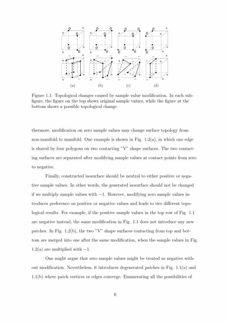
Figure 1.1 Topological changes caused by sample value modifi-cation. In each subfigure, the figure on the top showsoriginal sample values, while the figure at the bottomshows a possible topological change. 6
Figure 1.2 Topologies inconsistency caused by modifying samplevalues at contact points from zero to negative inexisting MC method. 7
Figure 2.1 15 cases in original marching cubes where dotsrepresent cell vertices with different sign, figure from[1]. 14
Figure 2.2 A hole between two adjacent cells. The figure is from[2]. 15
Figure 2.3 Two cases of a cell face with diagonal positive verticesand diagonal negative vertices. 15
Figure 2.4 Possible tunnel connection within a cell. The figure isfrom [2]. 16
Figure 2.5 An example of one possible way to find 2 patches in acell by exploring cycles. 18
Figure 2.6 13 cases of squares with zero cell vertices. 20
Figure 2.7 Bilinear interpolation results of 13 cases in Fig. 2.6 21
Figure 2.8 15 cases in original MC method can be solved byZMC correctly. 22
Figure 2.9 Solving zero edges. Four cell faces are unfolded withpossible zero edges on a cell face A. 24
Figure 2.10 Solving ambiguities in case 4, 8 and 11 of Fig. 2.6.Two cell faces incident on the zero edge are unfolded,in which solid line stands for patch edge while dottedline for undecided patch edge. 25
Figure 2.11 Solving ambiguities in case 12 of Fig. 2.6. Solid anddotted lines stand for patch edge. 26
xii

LIST OF FIGURES—Continued
Figure 2.12 Insert a zero face between two adjacent cells repre-sented by the shaded region. 28
Figure 2.13 An example of volume and surface. 30
Figure 2.14 Case 10 initially has 8 possible ways to connect patchedges. 31
Figure 2.15 One original case Q = 227 and its corresponding caseswith zero vertices. 33
Figure 2.16 Topologies comparison on case 12 in Fig. 2.6: (a)Original topology (b) ZMC (c) Modified ZMC (d)Lewiner’s implementation. 34
Figure 2.17 Topologies comparison between ZMC and theLewiner’s MC implementation on cases 2 in Fig.2.7(a). 35
Figure 2.18 Depicting non-manifold surfaces by existing MCmethods. 36
Figure 2.19 Examples constructed by ZMC. 37
Figure 3.1 Instable segmentation results in (b) and (d), resultedfrom Two estimation of intensity distribution of a3D image in (a) and (c) respectively. The blue line isthe intensity histogram while red line the estimationresult. 41
Figure 3.2 One slice at z = 10 in the 3D image in Fig. 3.1. 42
Figure 3.3 Final 3D segmentation results by combining gradientinformation and intensity distribution on the slice atz = 10. 44
Figure 3.4 Segmentation results of a 3D lung image data. 3Dboundary surface reconstructed. 45
Figure 3.5 Segmentation results: 2D contour on one slice atz = 26 in blue lines. 46
xiii

LIST OF FIGURES—Continued
Figure 3.6 Segmentation results on nodule slices at z = 24and 33. (a) and (d) are the segmentation results byintensity distribution; (b) and (e) are the gradient;And (c) and (f) are the final result by the proposedmethod in blue lines. The red lines are the nodulecores manually marked by physicians. 47
Figure 3.7 Percentage of the 13 cases in one experiment. Theother cases include case 4 0.18%, case 7 0.02%, case8 0.01%, case 9 0.08%, case 10 0.28%, case 11 0.06%,case 12 0.0004% and case 13 0.39%. 50
Figure 4.1 The procedure of genus-zero shape classification. 52
Figure 4.2 A non-convex object maps to the same EGI as aconvex object, shown in 2D contour. 56
Figure 4.3 Original Models and their SNI. 57
Figure 4.4 The amplitudes of SH function for K = 0, 1, 2, 3 [3]. 58
Figure 4.5 Two abstraction levels of SOM method. The firstlevel is the set of prototype vectors. Using SOM tocluster the first level to get the second level. [4] 61
Figure 4.6 Shape classification result by SOM. 63
Figure 4.7 The 3D models in the prototypes. 64
Figure 4.8 SCI (top) and SGI (bottom). 65
Figure 4.9 The pose alignment results of cuboids. 65
Figure 4.10 Bunnies with different resolutions. 66
Figure 5.1 The procedure of general shape classification using 4DHSH and SVM. 68
Figure 5.2 Shape distribution of 5 tanks (gray) and cars (black).The figure is from [5]. 69
xiv

LIST OF FIGURES—Continued
Figure 5.3 The voxelization and intersection procedure ofconcentric spheres model (CSM). Figure on the leftis the original surface based model, while that in themiddle is voxel based model. And the figure on theright is the result after intersection with concentricspheres model. The figure is from [6]. 70
Figure 5.4 The right object is obtained by applying a rotation tothe inter part of the plane on the left. The figure isfrom [7]. 71
Figure 5.5 Surface based models and voxel based models. 72
Figure 5.6 (a) A separating hyperplane with a small margin.(b) A separating hyperplane with a larger margin.Solid dots and squares represent data in two classes.Dotted lines stand for the hyperplane boundary [8]. 76
Figure 5.7 The procedure of general shape matching using 4DHSH. 77
Figure 5.8 Bunny in three rotations. 79
Figure 5.9 Classification performance on random, concentricspheres model (CSM), and 4D HSH shape descriptors.Y axis indicates correct classification rate in percents.
81
Figure 5.10 An input model and its top 11 matched models. Theupper left with green frame is the input model, whilethe others are retrieved from database. Retrievedmodels with blue frame are in the same class as theinput model, while those with red frame are not. 82
Figure 5.11 Recall and Precision curve of random, concentricspheres model (CSM), and 4D HSH shape descriptorsfor the vehicle class in Set 2. X axis is recall while Yaxis indicates precision. 83
xv

LIST OF FIGURES—Continued
Figure 5.12 Recall and Precision curve of random, concentricspheres model (CSM), and 4D HSH shape descriptorsfor all classes average. X axis is recall while Y axisindicates precision. 84
Figure 5.13 Recall and Precision curve of for all classes withimprovement by pose alignment. X axis is recallwhile Y axis indicates precision. 85
Figure 5.14 Recall and Precision curve of random, concentricspheres model (CSM), and 4D HSH shape descriptorsfor shapes in Set 1. X axis is recall while Y axisindicates precision. 86
Figure 5.15 An input model and its top 19 matched models. Theupper left with green frame is the input model, whilethe others are retrieved from database. Retrievedmodels with blue frame are in the same class as theinput model, while those with red frame are not. 89
xvi

CHAPTER 1
INTRODUCTION
1.1 Motivation
With the increasing computing power of modern computers, 3D graphics
technologies find more and more applications in various fields. For example, 3D ani-
mation techniques can produce spectacular movie scenes that are difficult if not im-
possible by traditional techniques. Virtual reality graphics can help to train pilots
for planes or space shuttles. In computer aided diagnose, surface construction meth-
ods can render a 3D view of specific organs based on a series of CT scans to help
physicians evaluate the symptoms intuitively. The shape of physical objects can be
digitalized by laser scans into shape database, from which engineers design various
components using computer aided design (CAD) software.
3D graphics research covers broad areas including surface construction, shape
modeling, scene rendering, animation, user interaction, shape classification and match-
ing. 3D graphics technologies are popular topics in many subjects such as computer
graphics and vision, computational geometry and image processing.
3D shape analysis is the basis for many 3D graphics technologies. For exam-
ple, only with correct 3D shape model can one render a real sensed scene. This dis-
sertation focuses on 3D surface construction, shape classification and matching in
shape analysis. We will also discuss involved supporting technologies such as image
segmentation, conformal mapping and pattern recognition.
1

1.1.1 Surface Construction
Surface construction refers to the process in which an implicit surface is con-
structed from 3D volumetric data. It is an inevitable step for 3D data, such as seg-
mentation results on 3D image, to be evaluated intuitively by human eyes. Surface
construction is a widely studied topic in computer graphics and computer vision.
Polygonal meshes representing constructed surfaces are widely used in various ar-
eas, such as scene rendering and texture mapping. After surface construction we can
derive many geometric features, such as genus, curvature, surface area and volume,
which are basis for shape analysis.
An ideal surface construction should meet many requirements due to its im-
portance. First, the original topology of an implicit surface should be preserved. In
other words, the connectivity of surface parts should not be changed. Secondly, no
ambiguous surface should be generated, i.e. one and only one surface can be deter-
mined from a set of volumetric data. Thirdly, the generated surface is desired to be
adaptive to surface details. In other words, relative flat surface is represented by a
small number of big polygons while cute or detail rich surface is constructed by more
small polygons. Finally, surface construction method should be highly efficient for
large volumetric data.
Many surface construction methods have been proposed, but none meets all
the above requirements. Among them, marching cubes (MC) method, proposed by
Lorensen and Cline in 1987, is the most popular due to its efficiency in constructing
high resolution surfaces and simplicity in implementation [1]. But it also has defects,
such as topological ambiguities and representation inaccuracy. Surface construction
methods are being improved to meet its requirements.
1.1.2 Shape Classification and Matching
We can get 3D models through surface construction or through digitalization
of physical objects by laser scan techniques. The generated 3D models are widely
2

used in many fields of computer graphics, such as objects in animation scenes, com-
ponents in computer aided design (CAD), or protein chain in matching database. As
available 3D models on the Internet increase dramatically, efficiently searching rele-
vant shape models is desired by many applications.
Ideal shape classification and matching method should meet following require-
ments. Firstly, the method should find as many as possible 3D models similar to in-
put shape and exclude dissimilar ones. Secondly, it should eliminate variance from
pose difference of 3D models, such as shift, scale and rotation. Thirdly, retrieval re-
sults should be insensitive to noise, disturbance, and mesh resolutions of 3D models.
Finally, a hierarchical approach is desired for 3D models in multiple resolutions. In
other words, the method adopts coarse classification and matching for models in low
resolution, while fine classification and matching for those in high resolution.
Shape-based retrieval of 3D data has been an active research area in disci-
plines such as computer vision, mechanical engineering and chemistry. The perfor-
mance of 3D shape search engine, however, is far behind that of text, such as Google
search engine.
1.2 Related Work
1.2.1 Surface Construction
Among many existing surface construction methods, we only review those rel-
evant in our research in Marching Cubes (MC) methods. In the original MC method,
proposed by Lorensen in 1987, Nielson and Hamann reported an ambiguous case on
a cube face with two diagonally opposite positive vertices and two diagonally oppo-
site negative vertices [1][9]. They proposed an asymptotic decider to solve the am-
biguity. Chernyaev and Natarajan independently found an internal ambiguous case
under trilinear interpolation in a cube interior [2][10]. Chernyaev used 33 configura-
tions to discriminate the ambiguous cases, while Natarajan used the value of a body
saddle point to solve the ambiguity. Matveyev also addressed the internal ambigu-
3

ity by analyzing the types of surface intersections with a cube diagonal [11]. Nielson
made a comprehensive analysis of trilinear interpolation of isosurfaces, in which 56
ambiguous cases were characterized and classified into three levels [12]. And 9 cases
contain triangles entirely on a cell face, which may lead to non-manifold surfaces. In
the context of this dissertation, the term surface and isosurface are exchangeable to
each other.
To improve representation accuracy, Lopes and Brodlie added a small number
of key points in a cell interior [13]. These critical points help to represent different
surface topologies including tunnels inside a cell. Theisel used cubic Bezier patches
to represent exact contours of piecewise trilinear interpolation [14]. The exact con-
tours were then modified to be globally G1 continuous. To reduce representation
error around sharp geometric features, Kobbelt et al. proposed an extended MC
method by using extra information of normals [15]. And the extended MC method
was adopted in adaptive grids by Ju et al. in [16]. The adaptive approaches, such as
octree based methods, use a small step size around sharp geometric features while
reduce the number of polygons overall [17][18][19]. For the same purpose, Montani et
al. proposed a discretized MC method that merges small facets into large coplanar
polygons [20][21]. And Cuno et al. adopted a hierarchical approach based on radial
basis functions [22].
The MC method was originally applicable only to manifold surfaces, which
are locally homomorphic to a two dimensional disk everywhere. A polygonal mesh
representing a manifold surface should satisfy the continuity condition that a poly-
gon edge should be shared by exactly two polygons, or lie in an external face of the
entire volume [23]. Non-manifold surfaces, such as contacting or intersecting sur-
faces, contain edges of degree three, four or more. Bloomenthal and Ferguson pro-
posed to polygonize non-manifold surfaces by decomposing a cell into tetrahedras,
which requires multiple intersections per cell edge [24]. Hubeli and Gross extended
fairing operations on non-manifold models in a multiresolution approach [25]. In the
4

context of MC method, Hege et al. used a probability interpolation model to polygo-
nize non-manifold surfaces [26]. Their look-up table was adopted by Yamazaki et al.
in a MC method based on discontinuous distance field for non-manifold surfaces [27].
However, one of the original MC assumptions, in which sample values should
be nonzero after thresholding, has not been addressed by existing MC methods. In
other words, it is assumed cell vertices lie either inside or outside an isosurface, not
on the isosurface. Even in MC methods of non-manifold surfaces that contain mul-
tiple regions, an isosurface is still not assumed to pass through cell vertices. The
assumption was introduced to ensure that the number of cases an isosurface inter-
sects a cell could be easily enumerated. Otherwise, case enumeration in existing MC
methods are incomplete and too many cases need to be added. This assumption,
however, does not hold in some situations. For example, volumetric data generated
by level set method may contain zero sample values, i.e. isosurface of level sets pass
through grids. Integer-valued isosurfaces of integer-valued data sets or synthetic data
may also meet zero sample values. In one of our experiments in the later chapter
of this dissertation, the cases with zero sample values take up to 7% of total cases.
Actually, the assumption to exclude zero sample values is regarded as a technical
problem in [23], and one of the several major artifacts in most existing isocontour
software in [28]. Zero sample values are also discussed in [29], but no specific MC
method was proposed.
To handle the situation with zero samples, many existing MC methods mod-
ify zero sample values. For example, when level sets pass through grids, Han et al.
changed sample values at such grid points from zero to negative [28]. This kind of
modification has defects from following aspects.
First, it may introduce obvious topological changes or representation error
to an isosurface, as shown in Fig. 1.1. Changing zero sample values in the top row
of Fig. 1.1 to negative introduces patches as shown in the bottom row of Fig. 1.1.
Thick lines in the figure represent intersections of isosurfaces and a cell face. Fur-
5
0
+
++
+
−−
−−
0
0
+
++
+
0
(a)
−
0
0
+
+ 0
0
0
+
+
+
+
− −−
−
(b)
0
+
+
− −
−−
−
−
0
0
+
+ 0
00
(c)
−
00
00
++
+
+
++
+
+−−
−(d)
Figure 1.1: Topological changes caused by sample value modification. In each sub-figure, the figure on the top shows original sample values, while the figure at thebottom shows a possible topological change.
thermore, modification on zero sample values may change surface topology from
non-manifold to manifold. One example is shown in Fig. 1.2(a), in which one edge
is shared by four polygons on two contacting ”V” shape surfaces. The two contact-
ing surfaces are separated after modifying sample values at contact points from zero
to negative.
Finally, constructed isosurface should be neutral to either positive or nega-
tive sample values. In other words, the generated isosurface should not be changed
if we multiply sample values with −1. However, modifying zero sample values in-
troduces preference on positive or negative values and leads to two different topo-
logical results. For example, if the positive sample values in the top row of Fig. 1.1
are negative instead, the same modification in Fig. 1.1 does not introduce any new
patches. In Fig. 1.2(b), the two ”V” shape surfaces contacting from top and bot-
tom are merged into one after the same modification, when the sample values in Fig.
1.2(a) are multiplied with −1.
One might argue that zero sample values might be treated as negative with-
out modification. Nevertheless, it introduces degenerated patches in Fig. 1.1(a) and
1.1(b) where patch vertices or edges converge. Enumerating all the possibilities of
6

0
−
−
+
−
+
+ −
−
−
0
+− −
−
− −
−
−
+
−
+
+ −
−
−
−
+
(a)
+ −
−
−
+
+
++
+
+
+
0
0
−
+−
+
−−+
+
+
++
−
−
+
−
(b)
Figure 1.2: Topologies inconsistency caused by modifying sample values at contactpoints from zero to negative in existing MC method.
degenerated patches in MC cases is also tedious. And it still brings obvious topologic
changes to Fig. 1.1(b), 1.1(c) and 1.1(d).
This dissertation proposes a more general MC method that does not mod-
ify sample values. It constructs isosurfaces by exploring cycles in two dimensions to
avoid enumerating all the cases directly [30]. We adopt bilinear interpolation and in-
troduce zero vertex, zero edge and zero face to solve ambiguous cases. The proposed
method is also applicable to some non-manifold surfaces.
1.2.2 Shape Classification and Matching
The comparison of shape similarity is the basis for shape recognition, classi-
fication and matching. In retrospect, similarity comparison methods have evolved
from 2D to 3D. 2D methods discriminate shapes based on 2D contours obtained at
different viewing angles. Most of them can not be generalized to 3D shape matching
directly. On the other hand, 3D methods extract shape features from 3D models to
match similar models [31]. Many survey papers summarized the development of 3D
7

shape comparison techniques [32][31][33]. As a large mount of 3D methods exist and
belong to various classes, we just mention a few related to our research.
Methods based on shape distribution enjoy the benefits of invariant proper-
ties and distinguish models in broad categories well. For example, shape distribution
method, proposed by Osada et al., is robust to translations, rotations, scales, mir-
rors, and tessellations [5]. However, they are not good at discriminating shapes that
have similar gross shape but vastly different detailed shape properties as indicated in
[31].
Spatial map based methods use map representation, which corresponds to
the physical locations of an object, and preserve the relative positions of features in
the object. They are able to capture detailed shape properties and have shown good
retrieval results [31]. For example, Hebert et al. used a deformed spherical mesh,
which was wrapped onto the 3D shape, and compared the shape similarity based
on geometric features on the sphere [34]. The method handles complex curved sur-
faces and supports partial matching. Nevertheless, it uses an expensive registration
step, in which data structures of all possible rotation of samples in the library are
pre-generated and stored. Moreover, shape estimation error was introduced during
reconstruction of original surface.
Among the spatial map based methods, spherical harmonic (SH) represen-
tation has been used in 3D shape modeling and retrieval [35][36]. Kazhdan et al.
used a rotation invariant SH representation based concentric spheres model (CSM)
in shape classification [7]. And Vranic proposed to use multiple radial distances in-
stead of volumetric values to preserve more surface details [37].
Methods based on 2D visual similarity require multiple views of a 3D ob-
ject [38]. Gu et al. proposed a 2D geometry image to represent a 3D mesh [39]. It
cuts the 3D mesh open and maps it onto a unit square. Based on geometry images,
Laga et al. proposed a shape matching method to save comparison of multiple 2D
views [40]. However, similar 3D shape models are not guaranteed to have the same
8

cut since there are multiple choices of cutting paths. As a result their geometry im-
ages may be quite different due to different cutting, adding variance to the similarity
comparison based on geometry images.
Extended Gaussian Images (EGI) uses normal vectors as geometric features
to compare shape similarity [41]. However, EGI is not unique to non-convex objects,
referred as an ambiguity problem, and EGI does not incorporate local spatial maps
either.
We propose a new shape similarity comparison method based on spherical
normal images (SNI). Normal vectors are stored in the conformal map of a 3D mesh
over a unit sphere, which is one to one mapping without cutting the 3D mesh open.
The overall approach follows the sequence of pose alignment, conformal mapping,
feature extraction, and similarity search. We use self-organizing map to classify 3D
models collected from the Internet. The proposed method applies to genus-zero ob-
jects that are sphere-like without holes or handles.
For general shape classification and matching, geometric features or processes
should not be limited to specific classes of shapes. For example, as object volume ap-
plies to only closed shapes, methods involving volumes need to convert open shapes
to closed shapes [42].
As for feature extraction processes, graph based methods represent geometric
features using a graph, such as model graphs, reeb graphs and skeletons [43]. As effi-
cient comparison of general 3D shapes using graph metrics is very difficult, they are
not suitable in our context [31].
The rotation invariant shape descriptors based on CSM cut a 3D object along
radii [7]. If internal components of the object rotate around the mass center, which
results a different object, the shape descriptor will not reflect this change. In other
words, the CSM shape descriptor is ambiguous to objects that differ in internal com-
ponents rotation. To solve this problem, we propose a new shape descriptor based
on 4D hyperspherical harmonics (HSH). It maps a 3D object directly onto a unit hy-
9

persphere without cut. The shape and matching processes using 4D HSH descriptor
involve voxelization, conversion from Cartesian coordinates to Polar coordinates, fea-
ture extraction, classification and matching.
1.3 Contributions
In this dissertation we proposed a new generalized marching cubes method
for isosurface construction.
• It allows zero values to prevail cell vertices after thresholding. Therefore the
proposed method best preserves the original topology and improves represen-
tation accuracy of isosurfaces that pass cell vertices, since it does not modify
sample values.
• By constructing isosurfaces with cycles in cells, it avoids enumerating a large
number of cases introduced by zero cell vertices.
• And the efficiency of the proposed ZMC method is comparable to that of exist-
ing MC methods in constructing isosurfaces.
We also proposed a new approach for 3D shape classification based on spheri-
cal normal images (SNI).
• The SNI incorporates local features by conformal mapping over a unit sphere
and is unique to each shape without ambiguity.
• The proposed method using SNI can discriminate collected shapes very well
and performs better than that using spherical curvature images or spherical
geometry images.
• The SNI based method is also robust to mesh resolution and pose variance.
• And we used the SVD method to compute SH offline to shorten the response
time of online retrieval.
10

For general shape classification and matching, we proposed a rotation invari-
ant shape descriptor based on 4D hyperspherical harmonics (HSH).
• The 4D HSH shape descriptor maps a 3D object onto a 4D unit hypersphere
without cut along radii, thus avoid the ambiguity introduced by components
with internal rotation.
• At the same vector length, the proposed 4D HSH descriptor performs better
than those based on concentric spheres model (CSM) in shape classification
and matching.
• We adopted support vector machine (SVM) in shape classification and inte-
grate classification predictions into shape distance weights in similarity com-
parison. Experiments show the distance weights improved shape matching per-
formance.
• We also used the SVD method to compute HSH offline to facilitate online re-
trieval response.
1.4 Organization of Dissertation
This dissertation is organized as follows. In Chapter 2, we briefly introduce
background information of marching cubes (MC), propose a new isosurface construc-
tion method, zero-crossing marching cubes (ZMC) and solve its ambiguous cases.
We also discuss non-manifold surfaces in this chapter. Then we verify ZMC cases
by experiments. Synthetic data is used in a series experiments to demonstrate the
correctness of ZMC method. Chapter 3 presents an application of ZMC method
on measured data, 3D image segmentation results. And we also compare its perfor-
mance with existing MC methods.
In Chapter 4 we discuss shape classification methods. The background of
pose alignment and spherical conformal mapping of a 3D meshes are briefly described
in Chapter 4. Then we propose a new feature, spherical normal image (SNI), for
11

shape classification. Spherical harmonic representation (SH) of SNI and self-organizing
map (SOM) is used in the proposed approach, which are discussed in following sec-
tions of Chapter 4. We also present experimental results and analysis.
Chapter 5 discusses general shape classification and matching. We briefly re-
view some popular shape classification and matching methods. Then we propose a
new shape descriptor based on 4D hyperspherical harmonics (HSH). We use support
vector machine (SVM) as the classifier and present experimental results and analysis
on classification and matching.
Chapter 6 concludes the proposed methods for surface construction, shape
classification and matching. We also discuss directions of future work related to this
research.
12

CHAPTER 2
SURFACE CONSTRUCTION
2.1 Introduction
Surface construction is a crucial step to analyze volumetric data. Even 3D
models represented by voxels in volume graphics needs surface construction to be
appreciated by human eyes.
The object of surface construction is to generate a mesh representing an iso-
surface. A mesh M is a pair (K, V ), where K is a simplicial complex representing
the connectivity of the vertices, edges and faces, thus determining the topological
type of the mesh, and V = v1, . . . , vm, vi ∈ ℜ3 is a set of vertex coordinates defin-
ing the shape of the mesh in ℜ3.
The input of surface construction is volumetric data, which has a sample
value associated with each grid point. Eight adjacent data samples enclose a cubi-
cal region, called a cell or unit cube. Cell corners are called cell vertices or grid
points. Samples at cell vertices are thresholded before surface construction. Here-
after sample value is referred as that minus a threshold. And we call a cell vertex
with positive/negative/zero sample value a positive/negative/zero cell vertex, which
lies outside/inside/on the implicit surface respectively.
In this chapter we discuss methods to construct a surface, the basis for shape
analysis in the later part of this dissertation. We begin with the most popular sur-
face construction method, Marching Cubes (MC), and elaborate our improvement on
MC methods. Various ambiguous cases and non-manifold surfaces are discussed.
13

2.1.1 Marching Cubes
If sample values are either positive or negative, the isosurface is limited to
intersect a cell in 28 = 256 ways since each of the eight cell vertices can lie either
inside or outside the isosurface. Under this assumption, zero sample values are either
avoided by carefully selected threshold or modified into small positive or negative
values.
By exploiting the symmetries in the 256 ways, Lorensen et al. summarized
the cases into 15 patterns, as shown in Fig. 2.1, in the original Marching Cubes
(MC) method [1]. Each case is encoded and stored in a lookup table. For a given
cell, it is classified into one of these 15 patterns based on its sample values. And a
piece of isosurface is generated from the lookup table. The whole isosurface is con-
structed piecewise after processing all the cells.
Figure 2.1: 15 cases in original marching cubes where dots represent cell verticeswith different sign, figure from [1].
14

2.1.2 Ambiguous Cases
Nielson et. al reported that a surface hole may be generated between two ad-
jacent cells as shown in Fig. 2.2 [9]. The hole is due to different connections of ver-
tices on the common cell face in the two adjacent cells. The cell face with two diag-
onal positive vertices and two diagonal negative vertices has ambiguous connections.
They proposed an asymptotic decider to solve this ambiguity.
Figure 2.2: A hole between two adjacent cells. The figure is from [2].
Let φ00, φ01, φ10 and φ11 represent sample values at the four corners of a
cell face. Value at a logical coordinate (u, v) is obtained by bilinear interpolation,
φ(u, v) = φ00(1 − u)(1 − v) + φ01(1 − u)v
+φ10u(1 − v) + φ11uv. (2.1)
−
+
+
−
(a)
−
+
+
−
(b)
Figure 2.3: Two cases of a cell face with diagonal positive vertices and diagonalnegative vertices.
15

From (2.1) it is easy to get that curve φ(u, v) = 0 is a hyperbola on a cell face
with diagonal positive vertices and diagonal negative vertices, as shown in Fig. 2.3.
We then compute the interpolation value at the intersection point of the hyperbola
asymptotes,
φ(u0, v0) =φ00φ01 − φ10φ11
φ00 + φ01 − φ10 − φ11. (2.2)
If φ(u0, v0) > 0 then positive cell vertices are connected as Fig. 2.3(a); Otherwise
they are separated as Fig. 2.3(b). As a result, 29 ambiguous cases are found and
solved with equation (2.2) in case 3, 6, 7 12 and 13 of Fig. 2.1 [9].
Chernyaev found that, if a cell interior is estimated by trilinear interpolation,
internal ambiguity, i.e. tunnel connection, may exist as shown in Fig. 2.4 [2].
Figure 2.4: Possible tunnel connection within a cell. The figure is from [2].
A squared inequality was proposed to detect whether tunnel connection exists or
not. And Chernyaev found 23 internal ambiguous cases in case 3, 4, 6, 7, 10, 12 and
13 of Fig. 2.1 [2].
2.2 Zero-Crossing Marching Cubes (ZMC)
16

2.2.1 Background
If sample value at a cell vertex is allowed to be zero, then each of the eight
cell vertices has three instead of two possible positions relative to an isosurface, i.e.
inside, outside or on the isosurface. Thus the isosurface intersects a cell in a total of
38 = 6561 ways. To enumerate all these cases and reduce their symmetries manu-
ally, as what has been done in [1], are extremely tedious and error-prone to human.
Without modifying sample values we are going to eliminate the original assumption
of excluding zero vertices, which is used by existing MC methods. To avoid enumer-
ating all the 6561 cases directly, we go back to check two dimensional cases instead.
We name the proposed method zero-crossing MC method (ZMC).
A vertex in the mesh of an isosurface is the intersection point of the isosur-
face and a cell edge. The vertex position is obtained by linearly interpolating sample
values of adjacent cell vertices so that the constructed isosurface is close to the de-
sired object boundary. Vertices at two ends of a cell edge are adjacent. ZMC method
starts from two basic assumptions as following.
Separation Assumption If two adjacent cell vertices are positive and negative re-
spectively, an isosurface passes between them once. The two cell vertices are sepa-
rated.
Connection Assumption If two adjacent cell vertices are both positive or nega-
tive, an isosurface does not pass between them. The two cell vertices are connected.
Theoretically, an isosurface can pass through two adjacent cell vertices with
opposite sign in odd number of times. We introduce the above two assumptions to
ensure smoothness of the isosurface. As for a zero cell vertex, the isosurface may or
may not pass through it. An isolated zero cell vertex can be regarded as a degener-
ated isosurface. We will discuss zero cell vertices later.
17

For convenience of discussion, we define some terms that will be used fre-
quently in the discussion. A patch is the close intersection of an isosurface and a
cell, a polygon formed by connecting adjacent surface mesh vertices. A patch edge is
the intersection of an isosurface with a cell face, whose end points are two adjacent
surface mesh vertices on the cell edge. And a vertex degree is the number of patch
edges incident on the surface vertex within one cell. Note the vertex degree here is
different from typical definitions of the vertex degree, which is the total number of
patch edges incident on the vertex. The vertex degree here only counts patch edges
in one cell.
The definition of topology can be found in [44]. In this paper we use topology
to abstract inherent connectivity of objects depicted by their boundaries or isosur-
faces. Modifying zero sample values or regarding them as positive or negative ones,
as shown in Fig. 1.1 and 1.2, may change this connectivity property.
2.2.2 ZMC Procedure
(1) (2) (3)
(4) (5) (6)
Figure 2.5: An example of one possible way to find 2 patches in a cell by exploringcycles.
18

As mentioned in Section 2.2.1, a cell may hold patches in 6561 different ways
if taking zero cell vertices into consideration without excluding symmetric cases. In-
stead of enumerating all these cases, we go back to two dimensions to examine all
the possible cases of how an isosurface may intersect a cell face, i.e. how a patch
edge may be created. As a patch is enclosed by patch edges, the enclosure forms a
graph cycle that uses each graph edge exactly once. This suggests patches in a cell
can be found by exploiting cycles in the cell. The basic idea of ZMC method is fol-
lowing. We start from any of the surface vertices, find another coface surface vertex
if possible, draw a patch edge between them, and continue with the found vertex un-
til we return to the original vertex. After one cycle, or a patch, is completed, repeat
the process until all the patch vertices in the cell have been visited. Then we find
all the patches in the cell. An example of one possible way to find 2 patches is illus-
trated in Fig. 2.5.
However the procedure brings two questions. The first one is, how to guar-
antee the procedure will return to the origin vertex? In other words, how to avoid
dangling edges? The second question is, how many ways there are to define patch
edges on a cell face and how to make our choice? As more than two surface vertices
may lie on a cell face, there are multiple ways to define the patch edges, in which the
constructed patches in the cell would be completely different.
2.3 ZMC Ambiguous Cases
To answer the first question, we check the cycles that form patches in a cell.
The cycles are separated without sharing common cell vertices since patches do not
intersect with each other in the cell. Obviously the cycles are a simple kind of Eule-
rian circuits. According to the Eulerian circuit condition, a graph has Eulerian cir-
cuits if and only if it has no graph vertices of odd degree. In other words, to ensure
that patches found by ZMC method are complete, the degree of surface vertex in
the cell should be even. We prove later that ZMC method generates even number of
19

(13)
++
+ +
(1)++
+ −
(3)
++
0 −
(5)++
− −
(6)
++
0 0
(4)
0+
0 +
0+
0 0
(7) (8)
++
+ 0
(2)
(9)0+
0 − 0
(11)(10)0+
−
0+
− + 0 0
(12)00 −+
− +
Figure 2.6: 13 cases of squares with zero cell vertices.
patch edges incident on each surface vertex in one cell. For the second question, we
use the result by Banks et al. in counting cases to produce substitopes in MC meth-
ods [29]. They enumerated 13 distinct cases in two dimensions with zero cell vertices
as shown in Fig 2.6, in which symmetries between positive and negative cell vertices
have been eliminated. Hereafter, we refer case number to that in Fig. 2.6, unless the
case number is explicitly stated otherwise. Many of these cases, however, allow am-
biguous ways to connect patch edges. We will discuss these ambiguous cases in the
following sections. Below is a summary of our algorithm.
1. Use bilinear interpolation on a cell face to determine patch edges for 9 of 13
cases in Fig. 2.6.
2. Define zero edge in the rest 4 cases, i.e. case 4, 8, 11 and 12 in Fig. 2.6. And
solve ambiguity using two cell faces incident on the zero edge.
(a) Enumerate all the combinations of case 4, 8 and 11 for the two cell faces,
and determine patch edges based on the assumptions of separation and
connection.
(b) For case 12, use symmetry to reduce the number of configurations to 13,
and solve them using previous results and the two assumptions.
20

3. Define zero face and determine when to insert a zero face for cases involving
case 11 and 12.
2.3.1 Bilinear Cases
If the underlying functions of an isosurface are known, we can easily deter-
mine the correct topology of the isosurface and the corresponding patch edges. In
case that sampled data is obtained through physical measurements, it is often im-
possible to know its true topology. And various methods have been proposed to
solve the ambiguity of the topology.
We first adopt bilinear interpolation as in (2.1) to solve the ambiguity [9]. It
satisfies the separation and connection assumptions and solves most cases in Fig.
2.6, as shown in Fig. 2.7(a). The choice between ambiguous sub-cases 13.a and 13.b
can be made according to (2.2) by the asymptotic decider method proposed in [9].
Hereafter sub-case of a case is indexed by an alphabetic letter attached to the case
number.
(2)++
+ +
++
+ 0
+
+
(3)+
−
0+
0 −
(9)0+
0 +
(7) (10)0+
+−
(13.a)−+
− +
++
0 −
(5)++
− −
(6)
(13.b)−+
− +
(1)
(a) 10 successful cases.
+
0
(11)0+
− 0 0
(12)00+
0 0
(4)0+
0 0
(8)
(b) 4 unsuccessful cases.
Figure 2.7: Bilinear interpolation results of 13 cases in Fig. 2.6
21

(0) (1) (2) (3)
(4) (5) (6) (7)
(8) (9) (10) (11)
(12) (13) (14)
Figure 2.8: 15 cases in original MC method can be solved by ZMC correctly.
Case 1, 3, 6, 13.a and 13.b of Fig. 2.7(a) correspond to all the 15 cases in the
original MC method [1]. To show that the proposed method covers all the cases of
the original MC method, we use the 15 cases in the original MC method as input of
ZMC method and get the same patches in Fig. 2.8 as those in Fig. 2.1 , though the
triangulation is different. ZMC method also generates the same results for all the
possible configurations with ambiguous faces as those in [9]. Due to page limit, we
do not list the result here.
Note that the proposed method uses bilinear interpolation to determine ver-
tices connections by patch edges on a cell face. It finds patches by cycles without
specifying underline functions inside a cell and constructs isosurfaces piecewise. ZMC
22

method does not use trilinear interpolation, by which an internal ambiguity might
exist with a tunnel connection inside a cell [2].
With the bilinear interpolation of cell faces, we have the following case rule
for cases with zero cell vertices.
Case Rule of Bilinear Interpolation Using Fig. 2.7(a), we can determine the
patch edges of case 1,2,3,5,6,7,9,10 and 13.
2.3.2 Zero Edge Cases
However, ambiguities in case 4, 8, 11 and 12 are not solved well by the bilin-
ear interpolation, as shown in Fig. 2.7(b). In case 11, one patch edge intersects an-
other between its endpoints, resulting in a discontinuous isosurface. And patch edges
between two adjacent zero cell vertices, which are called zero edges, are not ensured
to lie on the boundary of two regions with different signs.
To avoid separating two regions with the same sign, both cell faces incident
on a possible zero edge should be checked. For example, to connect a zero edge α on
a cell face A, as shown in Fig. 2.9, we need to check both the cell face A and B in-
cident on α. The zero edge in case 11 is converted to either an edge β or γ to avoid
self-intersection, where β or γ separates a positive or negative cell vertex from the
rest of a cell face. To restate the problem, let SF (e) represents the set of face con-
figurations, in which a cell face F contains a patch edge e. We need to solve SA(α),
SA(β) and SA(γ) for case 4, 8, 11 and 12.
According to the definitions of α, β, and γ, we have the following properties.
Property 1 SA(α) = SB(α).
Property 2 SA(α)∩SA(β) = Ø, SA(α)∩SA(γ) = Ø, and SA(β)∩SA(γ) = Ø.
Property 3 SA(β) ∩ SB(γ) = Ø and SA(γ) ∩ SB(β) = Ø.
Property 1 indicates criteria to draw a zero edge α is equivalent in the adjacent cell
faces A and B incident on α. According to Property 2, α, β and γ are repulsive to
23

0
0
A B CD
x3
β
γα δ
x2
y2
x1
y1 y3
Figure 2.9: Solving zero edges. Four cell faces are unfolded with possible zero edgeson a cell face A.
each other, i.e. at most one of them appears on a cell face. If A and B are of case
11, as shown in Property 3, they both separate positive cell vertices or negative cell
vertices.
If we regard cell vertices at the two sides of a zero edge adjacent, we can de-
cide patch edges based on the separation and connection assumptions in Section
2.2.1. We only need to check the combinations of adjacent cell faces of case 4, 8, 11,
and 12 incident on α.
2.3.2.1 Case 4, 8 and 11
The results for the combinations of case 4, 8, and 11 are shown in Fig. 2.10,
with symmetries between positive and negative vertices eliminated. Only the two
cell faces incident on a zero edge among the six cell faces are used in solving zero
edges. For simplicity, we unfold the two cell faces incident on the zero edge and enu-
merate their cases in 2D. For example, case 4 has five sub-cases from 4.a to 4.e with
regard to cell faces incident on a possible zero edge. Note a case with two different
ambiguous faces are indexed by two labels accordingly. For example, the second sub-
figure in Fig. 2.10 contains cell faces of case 4 and case 8, which is indexed by 4.b or
8.a respectively. As each of the sub-cases of case 8 has two potential zero edges, we
need to check two combinations of the adjacent cell faces incident on the two poten-
tial zero edges respectively.
24

For ambiguous sub-cases 11.c.1, 11.c.2, 11.e.1 and 11.e.2, we want positive
vertices to be connected if positive sample values take dominance. Therefore, if the
absolute product of positive sample values is no less than that of negative ones, we
choose 11.c.1 and 11.e.1, otherwise 11.c.2 and 11.e.2.
(11.e.1)
(8.e) (8.f)(11.e.2) (8.g) (8.h)
00
+ 0
−0
00
+ 0
0−
00
+
+
0
0
00
+
+
0
0
00
+
+
−
−
00
+
+
−
0
00
+
+
−
−
(11.b,8.c) (11.c.1)
00
+
+
−
−
00
+
+
−
0
(11.c.2) (11.d,8.d)
00
+
+
−
−
00
+ +
+ 0
00
+ +
+ +
(4.a)
00
+ +
+ −
(4.b,8.a) (4.c,11.a)
00
+ +
0 −
00
+ +
− −
(4.d,8.b) (4.e)
Figure 2.10: Solving ambiguities in case 4, 8 and 11 of Fig. 2.6. Two cell faces inci-dent on the zero edge are unfolded, in which solid line stands for patch edge whiledotted line for undecided patch edge.
2.3.2.2 Case 12
The results for the combinations with case 12 are shown in Fig. 2.11. Due
to symmetry, the other eight cell vertices in the cell consist of 13 distinct configura-
tions as shown in Fig. 2.6, we only need to solve these 13 configurations and illus-
trate them directly in 3D. Fig. 2.11 shows patch edges for the twelve sub-cases of
case 12 in 3D. Note sub-case 12.a represents the configurations in which the other
25

eight vertices in the cell are of the case 1, 2, 4, 7, 8 or 12 in Fig. 2.6. To select be-
tween ambiguous sub-cases, we want positive vertices to be connected or take more
space if positive sample values take dominance. Therefore, if the absolute product of
positive sample values is no less than that of negative ones, we choose 12.d.1, 12.e.1,
12.g.1 or 12.h.1, otherwise 12.d.2, 12.e.2 or 12.g.2 or 12.h.2.
−
00
00
+
−−
+
00
00
−−
++
0
00
+0
0−
00
0 00
+0
−
00
000
+0
−
00
00
+0
+−
00
000
−
+0
00
00
−+
+−
(12.d.1)
(12.f)
(12.h.2)
(12.a)0
0
00
0/+
0/+0/+
(12.d.2)
(12.g.1)
0/+
(12.b)0
0
00
+
−+
(12.e.1)
(12.g.2)
+
(12.c)0
0
00
++
0−
(12.e.2)
(12.h.1)
0
0
00 +
+−
Figure 2.11: Solving ambiguities in case 12 of Fig. 2.6. Solid and dotted lines standfor patch edge.
The procedure to get the results in Fig. 2.10 and 2.11 is presented in Ap-
pendix A. We get the following case rule.
Case Rule of Zero Edge Case 4, 8, 11 and 12 with zero edges can be solved ac-
cording to Fig. 2.10 and 2.11.
For previous example in section 1.2.1, Fig. 1.1(a) corresponds to case 7 in
Fig. 2.7(a) and case 4.a in Fig. 2.10. Fig. 1.1(b) corresponds to case 7 in Fig. 2.7(a),
26

case 8.a and 8.f in Fig. 2.10. Fig. 1.1(c) corresponds to case 8.f in Fig. 2.10. Fig.
1.1(d) corresponds to 12.a in Fig. 2.11. They generate no patches within the cell.
By solving all the 13 cases of Fig. 2.6 according to the case rules of bilin-
ear interpolation and zero edge, we can decide patch edges for all the 6561 cases in
3D. This answers the second question. To ensure that ZMC method can find all the
patches by exploiting the cycles in the cell, we have the following theorem.
Theorem If patch edges are determined by the case rules of bilinear interpolation
and zero edge, the degree of a surface vertex is either zero or two.
The proof is shown in Appendix B. Since a vertex degree is at most two, ZMC pro-
cedure visits a vertex at most once. In other words, midway vertices besides an ori-
gin vertex do not form any loops. So we can stop searching when all the surface ver-
tices in a cell have been visited. The surface vertex of zero degree is regarded as iso-
lated and simply ignored. This can answer the first question.
2.3.3 Zero Face Cases
In the case rules of bilinear interpolation and zero edge, an isosurface inter-
sects a cell face with zero cell vertices, or zero edges. Nevertheless, the intersection
may be a face, i.e. an entire patch lies on the cell face, which is called zero face.
Zero faces happen on cell faces of case 12, or cell faces of case 11 with different patch
edges in two adjacent cells. Similar to zero edges, to ensure a zero face is on the
boundary of two regions with different signs, two adjacent cells incident on the zero
face need to be checked. If we treat cell vertices in the two cells incident on a zero
face adjacent, we can derive the following case rule from the separation and connec-
tion assumptions in Section 2.2.1.
Case Rule of Zero Face
27

1. If a zero face of case 12 separates two regions of different signs, a patch is in-
serted between the two adjacent cells as illustrated by Fig. 2.12(a); Otherwise,
no patch is inserted.
2. If a cell face of case 11 results in a different patch edge in two adjacent cells, a
patch is inserted as shown in Fig. 2.12(b).
In Fig. 2.12(a), if the right cell contains all zero vertices, the zero face is not solved
in two cells. In such an extreme case with regions of zero vertices, we ”shift” the left
cell to right until the zero face can be solved. By inserting a zero face between two
adjacent cells, we avoid the duplication from generating a zero face in each cell. And
the zero face inserted between adjacent cells does not affect the theorem of vertex
degree in Section 2.3.2.
−
0
0
0
0++
++
−
−
−
(a) Case 12
0
0+
+
++
−
−
−
−
+
−
(b) Case 11
Figure 2.12: Insert a zero face between two adjacent cells represented by the shadedregion.
The orientation of patch vertices is adjusted to keep the patch normal point-
ing outward the isosurface consistently. Once all the patches are found, we complete
the whole front isosurface. As triangular meshes are extensively used in graphics ap-
plications, we triangulate patches by converting polygons to triangles. To avoid self-
intersections between patches within one cell [23], we add a new vertex, the average
28

of patch vertices, as a common triangle vertex for a polygon with more than three
edges.
Banks and Linton also counted cases with zero cell vertices in three dimen-
sions in MC methods by numerical algorithms [29]. They found 147 cases in total
with the symmetries between positive and negative vertices eliminated. However, it
is unrealistic to manually verify this result by comparing the 147 found cases with
the 6561 original cases. And they did not specify how to generate meshes for the
147 cases or their ambiguous cases. Hege et al. found 58 different topological cases
if a cell vertex belongs to three different types that are symmetric to each other
[26]. Nevertheless, zero vertex is not symmetric to positive or negative vertex. Their
enumeration does not cover cases with zero vertices as Banks and Linton do. And
Hege’s method does not include ambiguous cases either. The advantage of ZMC
method is to generate meshes by exploring cycles without enumerating all the 6561
cases. In Fig. 2.7(b), Fig. 2.10 ∼ Fig. 2.12, ZMC has 39 cases including ambiguous
cases, much less than the 147 cases by Banks and Linton.
2.4 Non-manifold Surface
Isosurfaces constructed by existing MC methods typically separate regions
with positive vertices from those with negative vertices. In other words, it is a bi-
nary space partition that generates only manifold surfaces. By modifying zero sam-
ple values into positive or negative values, existing MC methods convert a possible
non-manifold surface into a manifold surface. As shown in Fig. 1.2, contacting im-
plicit surfaces are either separated or merged if constructed by existing MC methods.
ZMC method is able to depict this type of non-manifold surfaces correctly
by preserving zero cell vertices. One example of volume and surface is shown in Fig.
2.13(a). At intersection A, the space is partitioned into four parts. ZMC method
depicts the intersecting sphere and square without separating or merging the two
surfaces.
29

A +−+0 0
− + −
(a) A sphere and a square of four space partitions.
A++
+ +0 0−
(b) A sphere and a square of three space partitions.
Figure 2.13: An example of volume and surface.
In the case rule of zero face, we insert no zero face between two adjacent cells
when cell vertices at two sides of a zero face are of the same sign. Consequently two
contacting surfaces with a common surface are merged into one. Nevertheless, the
merging effect may be not desirable in some applications. For example, when two
individual parts are assembled together, it would be better to keep their common
mating face in the mesh representation. This requires partitioning a space into three
regions. ZMC method can easily realize the partition by modifying the case rule of
zero face a little bit. We insert a zero face between two adjacent cells incident on a
zero face of case 12, regardless of the signs of cell vertices at two sides of the zero
face. To illustrate, we still use the sphere and square example in Fig. 2.13(b), in
which the square is viewed as a mating face of two parts. At the intersection A, the
space is partitioned into three parts. And the sphere in Fig. 2.13(b) is connected in-
stead of being separated by the square in the middle in Fig. 2.13(a).
30

(8)
0+
+−
0+
+−
0+
+−
0+
+−
0+
+−
0+
+−
0+
+−
0+
+−
(1) (2) (3) (4)
(5) (6) (7)
Figure 2.14: Case 10 initially has 8 possible ways to connect patch edges.
The limit of ZMC method in constructing non-manifold surfaces is inherited
from the separation and connection assumptions in Section 2.2.1. For example, case
10 initially allows 8 ambiguous ways to connect patch edges as shown in Fig. 2.14.
Way 1, 3 and 4 disobey the separation assumption, and way 5, 6 and 8 disobey the
connection assumption. Using bilinear interpolation, ZMC method only validates
way 2. Like most of existing MC methods, ZMC method prohibits edges from in-
tersecting inside cell face and solves ambiguous cases by manifold surface patches.
While existing MC methods modify zero sample values to convert non-manifold sur-
faces into manifold ones, ZMC depicts the original non-manifold topology correctly
using zero vertices, zero edges and zero faces. Due to the connectivity of volumetric
data, with zero vertices only ZMC method supports at most 2 contacting surfaces in-
cident on a zero vertex, such as Fig. 2.17(a). With both zero vertices and zero edges,
ZMC supports partitioning a space into at most 4 parts incident on a zero edge, such
as Fig. 1.2. And with zero vertices, zero edges and zero faces, ZMC can partition
a space into at most 8 parts with 12 zero faces incident a zero vertex, such as Fig.
2.19(d).
ZMC method supports less non-manifold surfaces than MC methods for non-
manifold surfaces [24][26]. Nevertheless, ZMC method keeps zero vertices to repre-
sent an isosurface more accurately than existing MC methods when the isosurface
31

passes through cell vertices. And ZMC method preserves the non-manifold topology
when surfaces intersect or contact at cell vertices.
2.5 Experiments and Discussions
In previous sections we presented the zero-crossing marching cubes (ZMC)
method, and discussed various ambiguous cases and non-manifold surfaces. We proved
in theory that ZMC method can solve all the ambiguous cases of cells with positive,
negative and zero vertices. In this section, we use simulations to test all the ambigu-
ous cases and prove the correctness of ZMC method in a series of experiments on
synthetic data. We will present experiments on measured data at next chapter.
2.5.1 Case Verification
The theorem of vertex degree in Section 2.3.2 guarantees that we can find
patch edges for all 6561 cases with zero vertices by exploiting cycles in one cell. In
the experiments we verify the result of ZMC method on the 6561 cases. Each case is
indexed by P =7∑
i=03i · pi, where pi = 0, 1, 2 (i = 0, 1, ..., 7) corresponds to zero,
positive and negative sample values respectively. The generated mesh for case P ,
ranging from 0 to 6560, is then rendered by Matlab and saved as pictures in JPEG
files, which are available online [45]. Although generating meshes for the 6561 cases
is very tedious for human, checking the pictures by hand is still doable. In each case,
the generated mesh satisfies the separation and connection assumptions without dan-
gling edges. ZMC method generates patches for the 6561 cases correctly.
To show the advantage of the proposed ZMC method, we compare it with an
existing MC method implemented by Lewiner et al. [46]. Lewiner’s implementation
is based on Chernyaev’s technique to solve the ambiguity problem on the cell face
[2]. It modifies zero sample values at cell vertices to small positive values, which con-
verts a case with zero vertices into one of the 256 original cases. The complete map-
ping relationship between the 256 original cases and the 6561 cases with zero vertices
is presented in [45], in which the original 256 cases are indexed in the way similar to
32

P . Let qi = 0, 1 (i = 0, 1, ..., 7) corresponds to negative and positive sample values
respectively. The 256 original cases are indexed by Q =7∑
i=02i · qi. For example,
case Q = 227 may be converted from 31 cases with zero cell vertices, 7 of which are
shown in Fig. 2.15 along with the original case Q = 227. The mesh presentation of
the case Q = 227 changes obviously after the modification on zero sample values. It
illustrates representation error of existing MC methods on implicit manifold surfaces
that pass cell vertices.
(a) Q = 227
−
0
0
0
−
0
0
−
(b) P = 234 (c) P = 235 (d) P = 2422
(e) P = 2424 (f) P = 481 (g) P = 2664 (h) P = 1206
Figure 2.15: One original case Q = 227 and its corresponding cases with zero ver-tices.
We also check ZMC method over ambiguous cases that are solved by compar-
ing the product of positive and negative sample values in case 11, 12 or 13. Based
on the comparison result, we choose from two possible results of an ambiguous face.
Let ri = 0, 1 (i = 0, 1, ..., 5) represents the two results of an ambiguous face i. The
index number R =5∑
i=02i · ri ranges from 0 to 63. For example, case P = 2422 in
Fig. 2.15(d) has two ambiguous faces of case 11 and 13. To enumerate its ambiguous
cases, let the two positive sample values be D1, D2 or D3, and the three negative
sample values be −D1, −D2 or −D3, where D3 > D2 > D1 > 0. With 32+3 = 243
33

enumerations, we find 2 ambiguous cases for case P = 2422. For the 6561 cases with
zero vertices, we find total 8447 ambiguous cases, which are indexed by P and R
[45].
−
0
0 0
0
−
−
−
−
−− −
0
+ +
++
+ +
++
0
0 0
(a) (b) (c) (d)
Figure 2.16: Topologies comparison on case 12 in Fig. 2.6: (a) Original topology (b)ZMC (c) Modified ZMC (d) Lewiner’s implementation.
For the case rule of zero face, we test ZMC method by enumerating all the
different combinations of two adjacent cells incident on the cell face of case 11 or
case 12 in Fig. 2.6. ZMC method works correctly on all these enumerations with re-
sults in [45]. On example of two cells incident on a cell face of case 12, is shown in
Fig. 2.16. ZMC method gives no zero face since the zero face are not on the bound-
ary of two regions with different signs. For the modified case rule of zero face in Sec-
tion 2.4, ZMC generates one zero face. ZMC method gives consistent results when
the cell vertices besides the zero face in the two adjacent cells are positive or nega-
tive. In comparison, Lewiner’s MC implementation outputs two planes for the top
case of Fig. 2.16. But it generates no plane when the sample values are multiplied
by −1 in the bottom case of Fig. 2.16. It shows preference to positive values since it
changes zero sample values to positive ones.
34

2.5.2 Non-manifold Surface
We compare Lewiner’s implementation and ZMC method over the cases in
Fig. 2.17. For the case shown in top row of Fig. 2.17, Lewiner’s method reports
eight times of case 2 of Fig. 2.8 and generates 16 triangles. When the sample values
are multiplied by −1 as shown in the bottom case of Fig. 2.17, Lewiner’s method
reports eight times of case 1 of Fig. 2.8 and generates 8 triangles. To illustrate, we
enlarge its small positive value to 0.05 and get the result in Fig. 2.17(c). Note this
enlargement does not change the topologies of constructed meshes or the number of
generated triangles. The proposed ZMC method consistently preserves the original
topology as shown in Fig. 2.17(b).
−
+
+
− −
− −
−−
−
0
+
0
+−
−
+ +
+
+
+
(a) Original Topology (b) ZMC (c) Existing MC
Figure 2.17: Topologies comparison between ZMC and the Lewiner’s MC implemen-tation on cases 2 in Fig. 2.7(a).
The example of non-manifold surfaces in Fig. 2.13, volume and square, are
constructed by Lewiner’s implementation in Fig. 2.18. Comparing with Fig. 2.13(a),
the sphere is converted into a bowl and a half sphere in Fig. 2.13(a). And the square
in Fig. 2.13(b) is removed in Fig. 2.18(b). Note the enlargement causes coarse sphere
35
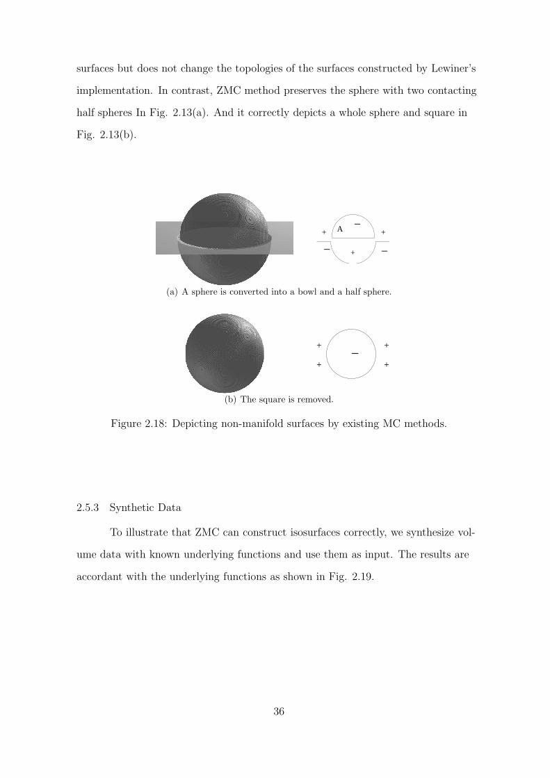
surfaces but does not change the topologies of the surfaces constructed by Lewiner’s
implementation. In contrast, ZMC method preserves the sphere with two contacting
half spheres In Fig. 2.13(a). And it correctly depicts a whole sphere and square in
Fig. 2.13(b).
+−A
+− −
+
(a) A sphere is converted into a bowl and a half sphere.
++
+ +−
(b) The square is removed.
Figure 2.18: Depicting non-manifold surfaces by existing MC methods.
2.5.3 Synthetic Data
To illustrate that ZMC can construct isosurfaces correctly, we synthesize vol-
ume data with known underlying functions and use them as input. The results are
accordant with the underlying functions as shown in Fig. 2.19.
36

(a) Three torus (b) Four spheres
(c) Drip (d) Case
Figure 2.19: Examples constructed by ZMC.
37

CHAPTER 3
VISUALIZING IMAGE SEGMENTATION
In Chapter 2, we presented the ZMC method and verify it on simulated cases
and synthetic data. In this chapter we apply ZMC method on measured data, 3D
image segmentation results. ZMC method was motivated by the need to visualize
3D image segment results from our new level set method. As level sets may pass
through grids, or cell vertices, existing methods modify zero-valued data [28], which
introduces topological changes as discussed in Section 1.2.1. Without changing data
values, ZMC method preserves original topology better and exhibits comparable per-
formance with existing MC methods on large volumetric data set.
In this chapter, we briefly introduce the background of an extensively used
image segmentation method, level set, and our improved 3D level set method. To
visualize 3D segmentation results, we apply ZMC method and conduct a series of
experiments to compare its performance with existing MC methods.
3.1 Level Set Method
Propelled by growing computing power, 3D image processing techniques find
increasing applications in medical domain, such as computer aided diagnose (CAD)
and computer aided surgery. As a key technology, 3D image segmentation became
a popular topic of medical image processing. Accurate 3D geometric information of
organic structures is crucial for early disease diagnose and treatment. However, seg-
mentation of some organic structures, such as lung bronchia and nodules, is a chal-
lenging task due to their complex topologies. We proposes a new automatic 3D im-
age segmentation method for these structures based on level set method.
38

Level set method, proposed by Osher and Sethian, has been extensively stud-
ied and widely used in image segmentation [47]. Many variations have been proposed
to improve the level set method. One branch of level set methods, fused the various
regional statistics like intensity distribution, can enhance segmentation capabilities.
For example, Baillard et al. incorporated pixel-classification based on intensity dis-
tribution into the level set speed function [48]. Their automatic method gave impres-
sive segmentation results on brain images. To estimate distribution of incomplete
data, Dempster et al. proposed an expectation-maximization (EM) framework [49],
which has been adopted in many later approaches such as [50]. And a stochastic EM
(SEM) algorithm, was proposed by Masson and Pieczynski to reduce the dependence
on initialization of the EM method [51]. However, both the EM and SEM method
do not guarantee the global optimal estimation and or eliminate the dependency of
estimation results on initialization. The estimation error in intensity distribution can
make segmentation results instable as shown in the later sections of this chapter. We
investigate the effects of the estimation error and propose a new calibrating mecha-
nism to combine gradient information and intensity distribution into segmentation
process. By searching the maximal overlap of image gradient with the boundaries
determined by intensity distribution, the proposed method can locate the boundaries
of interested objects more stably.
The central idea of level set is to represent boundaries of different regions by
a moving front γ(t), which converges to the desired boundaries from its initial po-
sition. The moving front γ(t) is a zero level set of a higher dimensional function
ψ(x, t), x ∈ ℜN , and represents a closed hyper-surface. It is propagated along its
normal direction by updating ψ(x, t) according to some criteria. The ℜN space is
then divided by the moving front, into the region Ω enclosed by γ(t) and the outside
region Ω, which satisfy: ψ(x, t) < 0, x ∈ Ω;ψ(x, t) = 0, x ∈ γ(t);ψ(x, t) > 0, x ∈ Ω.
The evolution equation for ψ(x, t) is given as
39

ψt + F |∇ψ| = 0, (3.1)
where F is the speed function of the moving front. A typical speed function is in the
form of:
F = kI (FA + FG), (3.2)
where kI = 1/(1 + |∇Gσ ∗ I(x)|m) reflects the stopping criteria by image gradient,
FA is an advection term independent of the moving front’s geometry, and FG is a
speed term dependent on the geometry such as local curvature.
The speed function should decrease to zero quickly when the front meets ob-
ject boundaries. It suggests a large m in kI if using image gradient as the only stop-
ping criteria. Nevertheless, with a large m the front is likely to stop at regions with
middle gradient, which may be noise or textures, instead of object boundaries in an
image. On the other side, with a small m level set may leak into object boundaries
whose gradient is low.
3.2 Intensity and Gradient Combined Level Set
Using intensity distribution into the level set speed function, instead of image gra-
dient, eliminates the need to adjust m, thus makes segmentation automatic. It can
detect object boundaries with low gradient or reduce noise effect in gradient. How-
ever, an accurate and stable estimation of intensity distribution is difficult to get
from a finite set of 3D image data. The EM or SEM method does not guarantee
convergence, or find the global optimum, whose results depend on the initialization.
Consequently, the segmentation result based on intensity distribution may be insta-
ble. For example, by running the SEM algorithm twice on a 3D lung image of size
80 × 80 × 28, we get two estimation results of its intensity distribution, as shown in
Fig. 3.1(a) and 3.1(c). Note the estimation results around the left peak are differ-
40

0 50 100 150 200 250 3000
0.01
0.02
0.03
0.04
0.05
0.06
0.07
0.08
0.09
0.1
(a) (b)
0 50 100 150 200 250 3000
0.01
0.02
0.03
0.04
0.05
0.06
0.07
0.08
0.09
(c) (d)
Figure 3.1: Instable segmentation results in (b) and (d), resulted from Two estima-tion of intensity distribution of a 3D image in (a) and (c) respectively. The blue lineis the intensity histogram while red line the estimation result.
ent in the two figures. Fig. 3.1(b) and 3.1(d) show the corresponding results of the
level set segmentation on a slice at z = 10. The inside region in Fig. 3.1(d) ”shrinks”
compared with that in Fig. 3.1(b), resulting some structures to break or disappear.
The original image of the slice and its gradient are shown in Fig. 3.2(a) and Fig.
3.2(b) for reference. Checking intensity values of different parts in Fig. 3.1, we find
the left peak corresponds largely to the background, the right two peaks correspond-
ing to lung walls, and the middle flat part corresponding to the organic structures
we are interested on, such as bronchia, vessels and the boundaries of lung walls. As
their intensity values are not distinctive from those of the background, a small dis-
turbance on the estimation result of intensity distribution, will change the segmenta-
tion result of the low intensity structures obviously.
To reduce the ”shrink” or ”expand” effect on segmentation results, we pro-
pose to use gradient information to calibrate the estimation of intensity distribu-
tion in the following. We compute the overlap of image gradient with the boundaries
determined by intensity distribution through introducing a probability offset to in-
41

tensity distribution. The maximum overlap indicates the optimal boundaries of the
interested objects.
(a) Original Image (b) Gradient
Figure 3.2: One slice at z = 10 in the 3D image in Fig. 3.1.
To restate the problem without losing generality, here we use a mixed Gaus-
sian distribution model,
P (u) =n
∑
k=1πkP (u
∣
∣
∣λk;µk, σk ), (3.3)
where πk is the prior probability of class λk withn∑
k=1πk = 1, and µk, σk are the
mean and variance of the Gaussian distribution of the intensity. We then get the
intensity distribution inside the region Ω,
Pin(u) =∑
k|λk∈Ω
πkP (u∣
∣
∣λk;µk, σk) . (3.4)
And the intensity distribution of the outside region Ω, Pout(u), can be obtained in a
similar way. Normally for pixel x on region boundaries with u = I(x), we have
Pout(I(x)) − Pin(I(x)) = 0. (3.5)
The final boundaries, where level set front actually stops, coincident largely with
those predicted by (3.5) in practice. As previously discussed, segmentation result by
42

level set methods based on intensity distribution requires an accurate estimation of
intensity distribution, while the global optimum of the estimation is not guaranteed
by existing EM methods.
To evaluate the estimation result of intensity distribution, we introduce a
probability offset w into equation (3.5) and define,
φ(x, w) = Pout(I(x)) − Pin(I(x)) − w, (3.6)
where the boundaries satisfy E(x, w) = x|φ(x, w) = 0. The value of w indi-
cates the reliability of segmentation results by intensity distribution. For example,
a negative w causes the segmentation result of inside region Ω to shrink, indicating
the probability of the inside region Ω has been overestimated. Actually, φ(x, w) is a
hyper-surface similar to the definition of ψ(x, t) in level sets, in which φ(x, w) = 0
represents object boundaries like level sets ψ(x, t) = 0 do. Define d(x, w) as the min-
imum distance from x to object boundaries and the according boundary detector is,
Ye(x, w) = e−d2(x,w), (3.7)
where Ye(x, w) = 1 for x on the boundaries and decreases exponentially with dis-
tance d(x, w). Different from the intensity-based boundary detector in [48], Ye(x, w)
takes the position x into consideration, indicating voxels in the center of an object
are less likely to be boundaries. As we expect the boundaries defined by intensity
distribution to overlap with image gradient as much as possible, define an objective
function as,
S(w) =∫
x(∇Gσ ∗ I(x))Ye(x, w)dx. (3.8)
The global overlap between the boundaries defined by the intensity distribution and
gradient is maximized, when
43

w = arg maxS(w)w
. (3.9)
Note that existing intensity distribution models assume w = 0. Furthermore, to
adjust boundaries locally, we define a factor kP = 1 − Ye(x, w) in the level set
speed function representing the boundaries defined by intensity distribution. The
final speed factor k combining both kI and kP can be designed in many ways. Gen-
erally, k is assigned a low value when both kI and kP are of low values, and a high
value when both kI and kP are of high values. Otherwise, k is a balanced value be-
tween kI and kP . To weight kI and kP automatically, we adopt a fuzzy logic table
similar to that in [52].
(a) The result of Fig.3.1(a)
(b) The result of Fig.3.1(c)
Figure 3.3: Final 3D segmentation results by combining gradient information andintensity distribution on the slice at z = 10.
To find w for equation (3.9), we search scope [−wsc, wsc] in multiple resolu-
tions, and the scope wsc is computed by,
wsc = C ·∫
u|P (u)−H(u)
H(u)|2du (3.10)
where C is an empirical constant and H(u) the normalized histogram at intensity u.
Actually, wsc prevents w converging to the boundaries of neighboring objects inside
or outside the current object.
44

The final segmentation results by the proposed method based on the two es-
timation of intensity distribution in Fig. 3.1(a) and 3.1(c) are shown in Fig. 3.3(a)
and 3.3(b) respectively. The difference between the two results is almost indiscernible.
Compared with Fig. 3.1(b) and Fig. 3.1(d), some noise in the gradient is filtered out
and the right side of the lung wall is preserved well where its gradient is low.
Lin et al. proposed to combine the distribution of both image gradient and
intensity [53]. But they did not consider estimation error in intensity and gradient
distributions.
The advantage of our method comes from using gradient information to cal-
ibrate the instable segmentation results, found by level set methods based on insta-
ble estimation of intensity distribution. It is helpful especially when the intensity
distribution is non-Gaussian, such as Rayleigh or Poisson distribution, where using
Gaussian model to estimate the intensity distribution may introduce large estimation
error.
3.3 Experimental Results and Analysis
3.3.1 Visualize Segmentation Results
Figure 3.4: Segmentation results of a 3D lung image data. 3D boundary surfacereconstructed.
45

Figure 3.5: Segmentation results: 2D contour on one slice at z = 26 in blue lines.
We test the proposed method on a series of CT lung scans downloaded from
the National Cancer Institute [54]. A narrow band level set method is implemented
to improve speed [47]. Time step is chosen adaptively to satisfy the Courant-Friedrichs-
Levy restriction to make segmentation stable. A user only needs to specify a box
containing the interested organic structures, or the region of interest (ROI). Using a
ROI with 290 × 380 × 62 voxels as the initial front surface, we get the segmentation
result with spacing 0.68, 0.68, and 0.63 mm along X, Y, Z axes.
To visualize the segmentation result, we construct a 3D boundary surface in
Fig. 3.3.1 using ZMC method. The thin structures like bronchia and fine surface
details are well captured. Note that some bronchia are not connected to the major
bronchial tree in this part of lungs. This is not resulted from the segmentation or
reconstruction error.
Another advantage of ZMC method is that 2D contours have already been
generated by patch edges within each patch. By collecting patch edges on every
plane, we can get the 2D contour at specified position, as shown for one slice at
z = 26 in Fig. 3.3.1. Ho et al. also constructed surfaces by finding 2D segments
in their CMS method [55]. But the CMS method does not consider zero cell vertices,
hence it inherits the topological artifacts of existing MC algorithms.
46

(a) (b) (c)
(d) (e) (f)
Figure 3.6: Segmentation results on nodule slices at z = 24 and 33. (a) and (d) arethe segmentation results by intensity distribution; (b) and (e) are the gradient; And(c) and (f) are the final result by the proposed method in blue lines. The red linesare the nodule cores manually marked by physicians.
From Fig. 3.3.1 and Fig. 3.3.1, it is easy to detect a nodule with many con-
nections in the left lung. We can re-assign the ROI to segment the nodule core. Fig.
3.6(a) and 3.6(d) show the segmentation results by the intensity distribution on
slices at z = 24 and 33 respectively. The gradient is shown in Fig. 3.6(b) and 3.6(e).
Fig. 3.6(c) and Fig. 3.6(f) show the segmentation results by the proposed method
for comparison. The inside regions of the nodule core were initially underestimated
by the intensity distribution, but calibrated by the gradient in the final results as
shown by the blue line. To compare with ground truth, we overlap the segmentation
results with the manual results by physicians in red contour [54]. From Fig. 3.6(c)
and 3.6(f), the two contours coincide very well. Note that it is difficult to segment
the nodule core by gradient information alone since the gradient around the nodule
core is not distinctive from that around the outline of the nodule.
In the experiments, we find that final segmentation results are decided largely
after the global calibration by w, indicating the role of local adjustment by the fuzzy
logic table is limited. In other words, w causes the boundary defined by intensity
47

distribution to shrink or expand globally to overlap with image gradient as much as
possible, which is essential to make final segmentation results stable. Nevertheless,
the proposed method can not ”correct” segmentation results when the SEM method
gives an estimation of intensity distribution that largely deviates from the true dis-
tribution. In practice, we run SEM method several times to select the best estima-
tion with the minimal wsc value.
The estimation of intensity distribution of the ROI with 290× 380× 62 voxels
takes about 29 seconds while the level set segmentation takes 15 minutes. The algo-
rithm has been run automatically over a total of 23 data sets and the results have
been validated by experienced physicians. Quantitative evaluation will be conducted
in the near future for the purpose of nodule classification.
3.3.2 Performance Comparison
As ZMC method processes more cases than existing MC methods, it is slower
than Lewiner’s implementation, which constructs isosurfaces by a pre-computed
lookup table. To speed up the construction process, we store the ZMC results of all
the 8447 ambiguous cases in Section 2.5.1 in a lookup table indexed by P and R.
For a specific case, instead of searching cycles, we compute its index number P and
R and retrieve the patches from the table. The running time depends on the size of
volumetric data, i.e. the number of voxels, and the specific isosurface. We use a se-
ries of volumetric data of different sizes from [54] and compare the running time of
ZMC method with Lewiner’s MC implementation, as shown in Table 3.1. From the
table, ZMC is a fast algorithm, which can generate about one million triangles per
second in the experiments. Its efficiency is comparable to that of Lewiner’s imple-
mentation. Note ZMC method produces around 70% more triangles than Lewiner’s
implementation do. The difference is due to a new common vertex added each patch
with four edges or more during triangulation. An alternative method to reduce the
number of triangles is to use an existing patch vertex as the common triangle vertex.
48

For example, the alternative method gives two triangles for a quadrangle instead of
four. Nevertheless, triangles generated by the alternative method depend on which
common vertex to use. And the alternative method may give a triangle on a cell
face, i.e. zero face in one cell, when three of the patch vertices are zero cell vertices.
It causes duplication or discrepancy among adjacent cells incident on the zero face
triangle. Further processing on this case and an adaptive approach in the future can
reduce the number of triangles.
Dimension VoxelNumber(106)
TriangleNumber(106)
Time(s)
MC210×320×36 2.33
0.31 0.45ZMC 0.50 0.59MC
512×512×28 7.051.12 1.42
ZMC 1.86 1.73MC
512×512×62 15.931.58 2.78
ZMC 2.62 3.34MC
512×512×103 26.634.36 5.5
ZMC 7.67 7.34MC
512×512×150 38.915.88 7.56
ZMC 10.42 9.88
Table 3.1: Running time of ZMC and Lewiner’s Implementation. Time are in sec-onds.
To get statistics of the 13 cases, we count their occurrence among the cells
that contain patches. Fig. 3.7 show the percentage of the occurrence of the 13 cases
in the third experiment with integer-valued samples of table 3.1. It indicates the
cases with zero vertices, case 2 and case 5, take 2% and 4%. Actually, the percent-
age of the 13 cases varies dramatically with volumetric data and experimental condi-
tions. All the experiments are carried out on an AMD Anthlon 64bit 3700+ proces-
sor with 2G RAM.
49

31%
2%
32%
4%
29%
1%Case 1Case 2Case 3Case 5Case 6Other cases
Figure 3.7: Percentage of the 13 cases in one experiment. The other cases includecase 4 0.18%, case 7 0.02%, case 8 0.01%, case 9 0.08%, case 10 0.28%, case 110.06%, case 12 0.0004% and case 13 0.39%.
50

CHAPTER 4
SPHERICAL NORMAL IMAGE
In Chapter 2 and 3 we discussed methods to construct surface of a 3D model
from volumetric data. As more and more 3D models are available, it is desired to re-
trieve 3D models with specific shapes efficiently. In a library, books are indexed into
various classes so that people can access a specific book quickly. Similarly, a way
to index 3D models is the key for shape classification and matching. Unfortunately,
3D models do not carry keywords with themselves, like titles, authors or subjects
of books. Geometric features of 3D models are used instead for representation and
classification purpose.
In this chapter, we discuss the shape classification process using a new fea-
ture, spherical normal image (SNI). It applies for sphere-like 3D models without
holes or handles, which are genus-zero objects. The process involves pose alignment,
conformal mapping, feature extraction using surface normals, and classification using
self-organizing map (SOM). The overall approach is shown in Fig. 4.1.
In the feature extraction step, SNIs are generated and used to index 3D mod-
els. We use a spherical harmonic (SH) representation of SNI to facilitate classifica-
tion process. We conduct experiments to test the effectiveness of SNI as a shape de-
scriptor and compare it with other geometric features like curvature and geometry
images. Multi-resolution support and the choice of classifiers are also discussed.
4.1 Pose Alignment
Traditional shape recognition methods that are based on geometric features
follow the strategy of registration and recognition. The registration eliminates the
51

Classes
over SphereSNI
Similarity Search&
Classification Spherical Harmonics
Feature ExactionUsing
PoseAlignment
Conformal Mapingover Sphere
Similar Shapes
Genus−Zero
Shape
Figure 4.1: The procedure of genus-zero shape classification.
variance of feature vectors caused by different poses. Factors to be considered usu-
ally include scaling, translation, and rotation. Translation is usually removed by
shifting the center of a mesh to the origin, and scaling is removed through normal-
ization. As for rotation, different methods have been proposed.
Hebert et al. proposed a pre-processing stage in which data structures of
all possible rotations of samples in a library are generated and stored [34]. This
method saves the time of pose alignment during online retrieval and enables par-
tial comparison of similar surfaces. Nevertheless, it requires an extra large storage
of samples at each possible rotation up to the resolution of a mesh. Kazhdan et al.
used a rotation invariant feature to avoid the rotation process [7]. Vranic compared
the shape comparison methods using principle component analysis (PCA) in pose
alignment and the methods without rotation processing, and concluded that the
PCA based methods have better performance [37].
The PCA method finds a set of orthogonal principle axes, on which projects
of original variables have the maximum variance. Principle axes are eigenvectors of a
covariance matrix of variables:
52

Cov =1
N
N∑
k=1(~Vk − E(~Vk)) × (~Vk −E(~Vk))T , (4.1)
where (~V1,~V2, · · · , ~Vk, · · · , ~VN ) are the original variables and E(~Vk) is the average.
Projects of the variable, or new variables, are generated by rotating the variable
around the average to the principle axes.
PCA method is efficient since it only involves eigenvector operations on the
matrix. However, two problems must be dealt with to apply PCA method in pose
alignment. First, if mesh vertices are used directly to calculate principle axes, the
result is sensitive to tessellation and resolution of the mesh. Second, PCA method
does not distinguish directions of principle axes.
For the first problem, Novotni et al. used mass distribution of the object, a
volumetric property, in the pose alignment [56]. Saupe and Vranic replaced the av-
erage with the gravity center ~C in their continuous PCA method (CPCA) [57]. Orig-
inal point set I is then translated to get a new point set,
I1 = I −−→C = −→U |−→U =
−→V −−→
C ,−→V ∈ I. (4.2)
And the covariance matrix is modified to be,
C =1
S
∫
I1
~U × ~UT du, (4.3)
where S is the surface area. As for the second problem, the directions of principle
axes are specified by multiplying the rotated result with a diagonal matrix,
F = diag(sign(fx), sign(fy), sign(fz)), (4.4)
where
fx =1
S
∫
I2sign(Vx)V 2
x dv, (4.5)
53

and fy, fz are obtained in a similar way.
We adopt the CPCA method in our pose alignment process, which works well
with most of the shapes collected from the Internet.
4.2 Conformal Mapping
To analyze geometric features of a 3D object, it is convenient to map the ob-
ject surface onto a region of a plane or sphere first. Surface analysis is then carried
over the plane or sphere domain. For a closed surface, mapping it onto a sphere, if
possible, yields less distortion than onto a plane.
Hebert et al. used a self-defined mapping in which a regular mesh initially
on a sphere is deformed to wrap a 3D object [34] . It captures the outline of the
3D object and supports non-zero genus object with holes or handles. However, it
introduces shape estimation error during surface reconstruction as original mesh is
deserted. Moreover, a regular mesh on sphere does not contain any geometric infor-
mation itself. Only nodes associated with its vertices contain geometric features of
the reconstructed mesh.
In contrast, conformal mapping is one-to-one and angle preserving. A mapped
mesh and the original mesh differ only in scaling factor in terms of the first funda-
mental form. In other words, shape is preserved locally in the sense that distances
and areas are only changed by a scaling factor [58]. Conformal mapping is used in
many applications such as texture mapping, remeshing and visualization. Many al-
gorithms have been proposed to calculate conformal mapping [59] [58]. Eck et al.
computed the conformal map of a 3D mesh by minimizing harmonic energy [59],
Eharm[h] =1
2
∑
i,j∈Edges(D)
ki,j ||h(i) − h(j)||2, (4.6)
where D is the 3D mesh and h is the conformal map. It can be interpreted as the
energy of a configuration of springs with one spring placed along each edge of D.
And the spring constants ki,j is defined as,
54

ki,j = −1
2(cot 6 α + cot 6 β), (4.7)
where α, β are the two angles opposite to an edge i, j in the two faces sharing the
edge. Gu and Yau proposed a non-linear algorithm to minimize the harmonic energy
[60]. If h is harmonic, the tangential component of the Laplacian at any point v of a
surface is zero, and constraints are added to make the result unique [61].
We adopt Gu and Yau’s algorithm to compute a conformal map over a sphere,
which is a six dimensional Mobius transformation group [60]. It translates the mass
center of a mesh to the origin to guarantee a unique mapping. For a non-convex
shape in which a vector starting from the origin may intersect a surface more than
once, the conformal mapping can converge to a valid mesh on a sphere without over-
lapping. Thus we avoid the ambiguity problem associated with EGI approaches.
Nevertheless, a conformal map over a sphere is limited to genus-zero shapes only. As
for non-zero genus shapes, they have to be cut open and mapped onto a plane [60].
4.3 Spherical Normal Image
Normal vectors have been used as geometric features in many shape analysis
approaches. They contain rich geometric information of the object. Tasdizen et al.
used normal vectors to smooth and reconstruct the original 3D object [62]. Gaus-
sian map based Extended Gaussian Image (EGI) is another example of using normal
vectors. EGI is translation-independent and has been widely used for classification
[41]. The constraints of EGI, however, lie in its mapping properties of ambiguity and
self-occlusion on non-convex objects. In other words, different non-convex shapes
may be mapped to the same EGI, and part of the surface may not contribute to EGI
mass on the sphere. Fig. 4.2 shows 2D contours of two 3D objects on the left and
right, with their common EGI in the middle.
To solve this problem, distributed EGI and complex EGI have been developed
to include more geometric information into EGI [63].
55

E
A
B
E
D
C
A
C
B
E
D
A
B
D
C
Figure 4.2: A non-convex object maps to the same EGI as a convex object, shown in2D contour.
In our approach, we take normal vectors ~N = Nx,Ny,Nz as the geometric
feature and store them in a conformal map over a unit sphere. SNI is generated by
interpolating grids of longitude and latitude. We use Gnomonic mapping to interpo-
late a grid point P inside a spherical triangle ABC,
P =uA+ vB + wC
||uA+ vB + wC|| , (4.8)
where 0 ≤ u, v, w ≤ 1 and u + v + w = 1. And P is given the same normal vector as
that of the original triangle ABC. To illustrate, we show Nx,Ny,Nz as R,G,B
color for shape models in Fig. 4.3.
Compared with geometry image, SNI incurs less distortion by mapping a
closed surface onto a sphere [39]. Without cutting meshes open, it also avoids the
variance resulted from different cutting paths among similar shape models. Com-
pared with the spherical parameterization proposed by Praun and Hoppe, which
minimizes stretch between an original mesh and the mapped mesh on a sphere [64],
SNI is based on a conformal map that preserves angles and local shapes. And SNI
does not need mapping from a sphere to a polyhedron or a unit square in [64], since
further classification on the SNI is carried out directly over the sphere without un-
folding.
56

(a) Ball (b) Cube (c) Bunny
Figure 4.3: Original Models and their SNI.
4.4 Spherical Harmonic Representation
In section 4.3 we generated a new feature, spherical normal image (SNI), to
represent a genus-zero shape. It is important that SNI preserves the crucial shape
information of a 3D model, so that we can use it to discriminate various 3D models
and find similar matches. In this section, a spherical harmonic representation of SNI
is used to facilitate classification. And we also discuss multi-resolution support for
coarse-to-fine classification.
Geometric features mapped onto the sphere, such as curvatures and normal
vectors, have been used in similarity comparison of 3D objects in many recognition
algorithms [34] [41]. They require the calculation of a composite distance between
substantial corresponding vertices of objects mapped on sphere.
For shape classification, indexing geometric features on a sphere can facilitate
comparison process. Schudy and Ballard used spherical harmonics (SH) to fit a sur-
face as a function over a sphere [65]. In our approach, the geometric feature stored
in a conformal map over a sphere, is regarded as a radial function f : S2 → ℜ. It
can be expanded as a linear combination of SH:
57

f(θ, φ) =∞∑
l=0
l∑
m=−lCml Y ml (θ, φ), (4.9)
where Y ml (θ, φ) is the SH and the coefficients Cml are uniquely determined by
Cml =∫ π
0
∫ 2π
0Y m∗l (θ, φ)f(θ, φ) sin θdφdθ. (4.10)
The original spherical function is therefore decomposed by a feature vector of coeffi-
cient Cml . Fig. 4.4 illustrates the amplitudes of SH functions for K = 0, 1, 2, 3 [3].
Figure 4.4: The amplitudes of SH function for K = 0, 1, 2, 3 [3].
We use SH decomposition of SNI to facilitate shape classification process.
The feature vector is constituted by SH coefficients Cml . In practice, we use the am-
plitudes of Cml in the feature vector and exclude those with m < 0 because of sym-
metries between Cml and C−ml . As N2x+N2
y +N2z = 1, the SH representation of Nz
58

is regarded as a redundancy and omitted. Therefore, the dimension of the feature
vector is (K + 2)(K + 1), where K is the highest order of SH. Feature vectors of a
ball, cube and bunny with K = 1 are shown in Table 4.1.
Ball Cube Bunny
Nx
C00 0.00243288 2.62533e-17 0.558153
C01 0.00178926 6.59502e-17 0.09185
C11 1.24949 0.8149 0.661967
Ny
C00 0.000376667 5.03471e-17 0.297591
C01 0.000429478 8.03768e-17 0.0311241
C11 1.5204 1.19423 1.001
Table 4.1: The feature vectors of a ball, cube and bunny with K = 1
Residual error Err is introduced by the truncation of higher orders of SH in
practice,
Err(K) =∞∑
l=K+1
l∑
m=−lCml Y ml (θ, φ), (4.11)
which decreases with the increase of the value of K, the highest degree of SH. Using
finite SH coefficients Cml is equivalent to apply a low pass filtering, whose level is
controlled by the K value.
In computing spherical harmonics, Li and Hero compared methods of singu-
lar value decomposition (SVD) and FFT [35]. SVD methods can be applied to ar-
bitrarily distributed sampling points, while FFT methods require uniform sampling
on latitude θ and longitude φ. Nevertheless, both methods give similar estimation
accuracy on same sampling data sets. Moreover, the complexity of SVD methods is
approximated as O(N3), while that of FFT methods is O(Nlog2N) [66], where N is
the number of sampling points.
However, it is the complexity of online computation of coefficients Cml , not
that of computing spherical harmonics, determines response time of online retrieval.
59

We use a SVD method to compute SH offline and only need to compute SH coeffi-
cients Cml for online retrieval to shorten response time. In appendix C we show that
both SVD and FFT methods have same complexity in online computation.
Multi-resolution meshes are desired for a coarse-to-fine classification. Dense
meshes contain highly detailed geometric information, which might be redundant
for coarse classification. They also incur excessive computation in the stage of map-
ping and feature extraction. Coarse meshes with basic geometric features are used
for first level classification; denser meshes with more detailed geometric features for
further classification.
Zhang and Hebert proposed a multi-scale classification approach [67]. It
adopts smoothed discrete curvature as local geometric feature. By varying the level
of surface smoothing, it compares the general shape similarity of two objects. This
method, however, loses many geometric features by smoothing surfaces in low scale.
Without smoothing the original surface, progressive mesh approach proposed by
Hoppe satisfies the need of multi-resolution support better [68]. It uses a simple
mesh M0 to represent an arbitrary mesh M , together with a sequence of edge split
records. To optimize the original mesh, an energy metric is introduced,
E(M) = Edist(M) + Espring(M) + Escalar(M) + Edisc(M), (4.12)
where Edist(M) equals to the sum of squared distances from points X = x1, · · · , xn
to the mesh, Espring(M) is the sum of spring energy placed on each edge, Escalar(M)
measures scalar attributes, and Edisc(M) measures geometric accuracy of its discon-
tinuity curves. Then it adopts edge collapse to minimize the energy.
We adopt the progressive mesh in our approach. And the size of feature vec-
tor is scalable to multi-resolution meshes, i.e. a shorter feature vector is used in
coarse classification and longer vector in fine classification. This scalability is achieved
by varying the highest SH order K.
60

4.5 Self Organizing Map
After feature vectors are obtained, we adopt a self-organizing map (SOM)
to classify 3D shape models [4]. Classifier selection is usually determined by sam-
ple data available and the specific application. Our research is focused on feature
extraction that is not limited to specific classifiers. Nevertheless, we have to check
classification performance to improve the design of feature extraction process. We
adopt self-organizing map (SOM) due to following reasons: (1) our shape meshes are
collected from the Internet, which are not pre-classified; (2) the definition of shape
class is subjective or fuzzy, for example, how to classify the sphere, cube, cone, tetra-
hedron and cylinder?
Self-organizing map is an excellent tool in exploratory phase of data min-
ing [4]. It is a two-level approach, of which the first level is a large set of prototypes
– much larger than the expected number of clusters. The prototypes are then com-
bined to form actual clusters as shown in Fig. 4.5 [4].
Figure 4.5: Two abstraction levels of SOM method. The first level is the set of pro-totype vectors. Using SOM to cluster the first level to get the second level. [4]
Usually the prototypes are arranged in 2D grid and each of them is repre-
sented by a prototype vectorMi = [Mi1, · · ·Mid], where d is the input vector di-
mension. At each training step, distance between sample dataX and all the proto-
61

type vectors are computed. The best-matching unit (BMU), b, is the one with proto-
type vector closest toX ,
|| ~X −Mb|| = min
i||X −
Mi||. (4.13)
And then the BMU and its topological neighbors are moved closer to the in-
put vector in the input space,
Mi(t+ 1) =
Mi(t) + α(t)hbi(t)[
X −
Mi(t)], (4.14)
where α(t) is an adaptation coefficient and hbi(t) is neighborhood prototypes cen-
tered on the BMU. The hbi(t) is computed as,
hbi(t) = exp(−||~Rb −Ri||2
2σ2(t)), (4.15)
where σ(t) is a coefficient like α(t), andRb and
Ri are positions of prototype b and
i on the SOM grid.
To visualize SOM result, the most widely used method is distance matrix.
The unified distance matrix, U-matrix, shows distance between prototype vectors
of neighboring map units. It can be visualized by gray shade or color. We adopt U-
matrix in our experiments.
4.6 Experiments and Discussions
We collect 3D models from various sources on the Internet, with acknowledg-
ment to SAMPL in Ohio State University [69], Princeton Shape Benchmark [70],
Vranic’s 3D Model Database [71] and Stanford 3D Scanning Repository [72]. Unfor-
tunately, current 3D model benchmark [70] is not applicable to our approach due to
the limit of genus-zero objects at present.
We extract feature vectors of 214 models with the highest SH order K = 16,
and use a SOM Matlab toolbox [73] to get the result of 12× 6 prototypes in Fig. 4.6.
62

0.0647
0.262
0.459
U−matrix
Labels
Fueltank
dean1.00
55
m619
m1608
glass1
m540
m360
93
mkwb.02
mkwb.01
1
33
135
4
54
Headstn
m1609
bunny
69
61
mraabe.
step.01
snub
27
102
127
52
106
51
45
cone
concave.
22
35
89
60
80
88
Ship2
Hex0
king
m1792
57
36
72
79
111
59
block4
94
29
128
58
41
3
82
63
76
132
47
Mush226
23
24
2
Figure 4.6: Shape classification result by SOM.
The left side of Fig. 4.6 is a U-matrix marked by different colors, while the right side
are prototypes with different labels. Blank label means no feature vector presents
in the prototype. As U-matrix displays distance between prototype vectors, feature
vectors with smaller distance means more similarity between the according 3D shape
models. And similar shape models should be clustered into the same or close proto-
types. By checking into prototypes, we find our method picks up similar 3D models
very well as shown in Fig. 4.7.
To compare the results of different feature vectors, we generate spherical cur-
vature images (SCI) and spherical geometry images (SGI) in a way similar to SNI
as shown in Fig. 4.8. Curvature inside a mesh polygon is computed by interpolat-
ing curvature at polygon vertices. And SGI is computed by interpolating normalized
X, Y, Z coordinates at polygon vertices. The method using SCIs requires dense
meshes and classifies cubes and balls into one prototype, whose SCIs resemble with
symmetries along X, Y, Z axes and large areas of constant curvature value. In con-
63

(a) Models in prototype labeled ’glass1’
(b) Models in prototype labeled ’23’
(c) Models in prototype labeled ’Hex0’
Figure 4.7: The 3D models in the prototypes.
trast, methods using SGIs and SNIs do not depend so much on mesh resolution and
can discriminate cubes and balls correctly. The method using SGIs yields occasional
”bad” classification compared with that using SNI. For example, a glass is found in
the prototype of cubes because its SGI is not distinctive from those of cubes.
The result of pose alignment can affect feature vectors and final classification
results. For example, for cuboids of 1 : 1 : 1 ratio in different initial poses, the PCA
method gives inconsistent rotations as shown in Fig. 4.9(a). Cuboids with 5 : 1 : 1
ratio are given inconsistent rotations along X axes in Fig. 4.9(b). Only those with
different ratio along X, Y, Z axes in Fig. 4.9(c) are registered consistently. The pose
variance of objects after registration decreases with asymmetries along X, Y, Z axes
64

(a) Ball (b) Cube (c) Bunny
Figure 4.8: SCI (top) and SGI (bottom).
increase, which is an artifact of registration using PCA methods. Nevertheless, the
effect of rotation on feature vectors is limited as shown in the experiments. The fea-
ture vectors of seven cubes are clustered into the prototypes labeled as ’1’, ’33’, and
’135’, which are very close according to the U-matrix in Fig. 4.6.
(a) 1 : 1 : 1 (b) 5 : 1 : 1 (c) 10 : 5 : 1
Figure 4.9: The pose alignment results of cuboids.
65

As for multi-resolution representation, we have generated different resolu-
tion meshes of same objects using Hoppe’s algorithms [68], such as bunnies in Fig.
4.10(a) and 4.10(b). The multi-resolution meshes of same objects are clustered into
same prototypes. It demonstrates that our method is robust to mesh resolution.
The SH representation is also used by Kazhdan et al. in their voxelized model
with 64 × 64 × 64 grids [7]. Fig. 4.10(c) shows the voxelized bunny of 15, 377 cubes
from the bunny of 4, 000 triangles in Fig. 4.10(a). Though using a much larger data
size, Fig. 4.10(c) loses many fine details of Fig. 4.10(a) before SH representation,
which is also addressed in [37]. Based on a surface based model, the proposed method
needs much smaller data size to present at least same level of surface details.
(a) Original Surface (b) High Resolution (c) Voxelized Model
Figure 4.10: Bunnies with different resolutions.
66

CHAPTER 5
GENERAL SHAPE ANALYSIS
In Chapter 4 we discussed shape classification by the spherical normal im-
age (SNI) based method. SNI preserves local geometric features using conformal
mapping on unit sphere and is unique to each 3D shape. The proposed SNI based
method discriminates collected shapes well in the experiments. However, due to the
limit of conformal mapping on sphere, SNI only applies to genus-zero objects, which
are sphere-like without holes or handles. To apply the SNI based method to gen-
eral shapes, we need to convert them to genus-zero objects first. Sphere-like mesh
wrapped onto the original object is a possible solution [34]. Nevertheless, shape esti-
mation error is introduced during reconstruction of original surface.
In this chapter, we are going to analyze general 3D shapes. We will review
classification methods for general shapes briefly. A new shape descriptor based on
4D hyperspherical harmonics (HSH) is proposed and compared with existing descrip-
tors. The shape classification process using proposed 4D HSH descriptor involves
voxelization, conversion grids from Cartesian coordinates to Polar coordinates, fea-
ture extraction and classification using support vector machine (SVM), as shown in
Fig. 5.1. We also discuss shape matching and conduct experiments to classify and
retrieve 3D shapes from shape benchmarks.
5.1 Introduction
As discussed in Section 1.2.2, many methods have been proposed for shape
classification and matching. To apply these methods to general shapes, however,
geometric features or processes should not be limited to specific classes of shapes.
67

Feature Extraction
Shapes
GeneralCoordinates
Cartesian−>PolarVoxelization
Hypersphere4D
Uisng 4D HSHUisng SVM
ClassificationShapes in
Predicted Classes
Figure 5.1: The procedure of general shape classification using 4D HSH and SVM.
For example, many spherical parameterization based methods require objects to be
genus-zero, which are closed surfaces without holes or handles [64].
We will briefly introduce popular shape classification and matching methods
for general shapes in the following sections.
5.1.1 Shape Distribution
Shape distribution methods use statistic geometric properties which can ap-
ply to general shapes [5]. For example, distance D2 refers to the distance between
two random points on a 3D object. The D2 histogram is then used as a shape de-
scriptor in discriminating different 3D shapes.
However, shape distribution based methods do not discriminate well objects
with similar gross shape but vastly different detailed shape properties [31]. Fig. 5.2
illustrates shape distribution of two classes of shapes, tanks and cars [5]. As their
gross shapes are similar, their shape distributions are difficult to be discriminated.
Extended Gaussian Image (EGI), which uses the histogram of normal vectors,
is known to be ambiguous to non-convex objects, as shown in Fig. 4.2.
68

Figure 5.2: Shape distribution of 5 tanks (gray) and cars (black). The figure is from[5].
5.1.2 Concentric Spheres Model (CSM)
Kazhdan et al. proposed a concentric sphere model and used rotation invari-
ant SH representation as the geometric feature for shape classification [7] [74]. They
first converted a given surface model into a volume model in 2R × 2R × 2R voxel
grid. A voxel is assigned value one if it intersects with the given surface, otherwise it
is assigned a value zero. Then the volume is intersected with R concentric spheres.
An illustration of the voxelization and intersection procedure is shown in Fig. 5.3 by
Vranic [6].
Recall from equation (4.9), the intersection of the volume with each sphere
can be viewed as a spherical function represented by SH. The amplitudes of SH rep-
resentation are used as the final shape descriptor,
SH(f) = ||f0(θ, φ)||, ||f1(θ, φ)||, ..., (5.1)
where fl is the frequency component of f ,
fl(θ, φ) =l
∑
m=−lCml Y ml (θ, φ). (5.2)
69

Figure 5.3: The voxelization and intersection procedure of concentric spheres model(CSM). Figure on the left is the original surface based model, while that in the mid-dle is voxel based model. And the figure on the right is the result after intersectionwith concentric spheres model. The figure is from [6].
With the definition in equation (5.1), the shape descriptor is independent of the ori-
entation of the spherical function,
SH(R(f) = SH(f), (5.3)
where R can be any rotation matrix [7]. In other words, we do not need to eliminate
rotation invariance in pose alignment since same objects in different rotation have
same shape descriptors. This rotation invariant property gives concentric spheres
model an advantage over methods requiring rotation elimination.
5.2 4D Spherical Harmonics Model
The concentric spheres model cuts a 3D object along radii into spheres. It
raises a problem that, if inner parts are rotated around the center, the shape descrip-
tor will not change at all. This is because the shape descriptor uses amplitudes of
SH representation which are rotation invariant according to equation (5.3). For ex-
ample, two different shapes in Fig. 5.4 have same shape descriptors [7]. The rotation
invariant property makes concentric spheres model ambiguous to shapes with rota-
tion of internal parts.
As rotation invariant property is desirable, we propose to eliminate this am-
biguity by treating a 3D object as a whole without cut along radii. Instead of using
70

Figure 5.4: The right object is obtained by applying a rotation to the inter part ofthe plane on the left. The figure is from [7].
concentric spheres model, we map the 3D object to a 4D unit sphere for analysis.
Accordingly we need 4D hyperspherical harmonic (HSH) to decompose the 3D ob-
ject and derive its shape descriptor.
5.2.1 Voxelization
Before we explore mapping relations between 3D and 4D space, let us exam-
ine the voxelization step in Fig. 5.1 first. As most of current available 3D models are
represented by polygonal meshes, which are surface based. The concentric spheres
model (CSM) based shape descriptor and the proposed 4D HSH shape descriptor
both require voxel based models. In other words, analysis is carried out on fixed
number of voxels, not polygons. We need to convert surface based model into voxel
based model, which is called the voxelization process.
The voxelization process is in reversed direction of surface construction pro-
cess we discussed in Chapter 2, in which we construct surface based models from vol-
umetric data. Many voxelization methods have been proposed for various usage [75]
[76]. Schroeder and Lorensen proposed to compute distance function for the genera-
tion of swept surfaces and volumes using implicit modeling [77]. Dachille and Kauf-
man limited the computation to voxels close to triangular meshes [78]. And Noorud-
din and Turk used voxelization techniques to simplify and repair polygonal meshes
[79].
71

As we only need to assign value one to voxels intersecting an input surface,
a simplified voxelization method can be adopted. We test each polygon in a sur-
face based 3D model to mark those voxels that have vertices at the both sides of
the polygon. To speed up the process, we only consider voxels that are close to the
polygon, similar to the distance criteria in [78]. Moreover, if the polygonal mesh is
coarse, we need to subdivide the mesh into smaller ones.
In our experiments, we convert surface models into voxel grids with size of
64 × 64 × 64, the same size as the one used in experiments of concentric spheres
models [80]. Fig. 5.5 illustrate the voxelization results of surface based models.
Figure 5.5: Surface based models and voxel based models.
Unlike concentric spheres models (CSM) shown in Fig. 5.3, we do not cut the
object along radii to compute intersections of the objects with spheres.
72

5.2.2 Coordinates Conversion
Similar to 3D unit sphere, a 4D unit sphere satisfies r = 1 where r is the dis-
tance to origin in 4D space. To understand 4D objects and space intuitively, Murata
and Hashimoto proposed an interactive environment [81]. In high dimensional space
spherical harmonics, or hyperspherical methods, have been explored to analyze n-
body quantum systems [82] [83]. Matheny et al. adopted 4D spherical harmonics for
time-dependent shape recovery and representation [84]. The 4th dimension in their
approach is time, not the 4th space dimension in our case.
Similar to 3D spherical coordinates, 4D hyperspherical coordinates r, θ0, θ
and φ, are connected to Cartesian coordinates as,
x = r sin θ0 sin θ cosφ y = r sin θ0 sin θ sin φ
z = r sin θ0 cos θ z0 = r cos θ0
(5.4)
where θ0 and z0 are the 4th dimensional coordinates. To compute hyperspherical
coordinates, we have,
r2 = x2 + y2 + z2 + z20 θ0 = ar cosz0r
θ = arctan
√
x2+y2
z φ = arctanyx
. (5.5)
5.2.3 Feature Exaction using 4D HSH
Similar to spherical functions represented by 3D harmonics in equation (4.9),
a hyperspherical function on 4D unit sphere can be decomposed as,
f(θ, φ, θ0) =∞∑
λ=0
λ∑
l=0
l∑
m=−lCmλ,lY
mλ,l(θ, φ, θ0), (5.6)
where Y mλ,l(θ, φ, θ0) is the 4D harmonics. It can be computed using 3D harmonics
Y ml (θ, φ) as,
73

Y mλ,l(θ, φ, θ0) = Nλ,lCl+1λ−l(cos θ0) sinl θ0Y
ml (θ, φ), (5.7)
where
Nλ,l = (−1)λil(2l)!!
√
√
√
√
2(λ+ 1)(λ− l)!
π(λ+ l + 1)!, (5.8)
and Gegenbauer polynomial Cαλ (u) is computed as,
Cαλ (u) =
[λ/2]∑
t=0
(−1)tΓ(λ+ α− t)
t!(λ− 2t)!Γ(α)(2u)λ−2t, (5.9)
in which Gamma function Γ(n) = (n− 1)! [83][85].
Similarly the shape descriptor is defined as,
HSH(f) = ||f0,0(θ, φ, θ0)||, ||f1,0(θ, φ, θ0)||, ..., (5.10)
where fλ,l is the frequency component of f ,
fλ,l(θ, φ, θ0) =l
∑
m=−lCmλ,lY
mλ,l(θ, φ, θ0). (5.11)
Note that rotation in 3D space only involves θ and φ. Therefore the new shape de-
scriptor is still independent of rotation in 3D space as depicted by equation (5.3).
In practice, the highest degree of HSH, K, is not infinite but truncated to
some finite value. Residual error is therefore introduced,
Err(K) =∞∑
λ=K+1
λ∑
l=0
l∑
m=−lCmλ,lY
mλ,l(θ, φ, θ0), (5.12)
which decreases with the increase of the highest degree of HSH, K. And the length
of 4D HSH shape descriptor is (K + 1)(K + 2)/2.
74

To compute 4D HSH coefficients Cmλ,l, we adopt an approach similar to that
in Section 4.4. The process uses singular value decomposition (SVD) to shorten on-
line retrieval response time as presented in Appendix D.
5.3 Support Vector Machine (SVM)
To evaluate the effectiveness of different shape descriptors, we need a classifier
to classify 3D shape samples into classes and then compare the results. In Section
4.5 we used self-organizing map (SOM) as the classifier. The main reason for this se-
lection is that no pre-classified data is available for genus-zero shapes. Fortunately,
several shape benchmarks provide pre-classified samples for general shapes [70] [71]
[86]. Therefore we can select a classifier that takes advantage of the pre-classified
samples. In our experiments, we adopted support vector machine (SVM) as the clas-
sifier.
SVM is a relatively new classification technique introduced by Vapnik et al.
in early 1990s [87] [88]. It has become one of the most popular classifiers due to its
superior performance in many applications. And it is an alternative to polynomial,
radial basis function and multi-layer perception classifiers.
The main idea of SVM is to maximize the margin between the classes with a
boundary. An example of linear classifier on two linearly separable classes is shown
in Fig. 5.6. The boundary in Fig. 5.6(b) is better with a larger margin between the
two classes.
SVM is derived from classical empirical risk minimization approach. Let us
look at a two classes recognition example. The task of a learning process is to con-
struct an appropriate set of decision functions fλ(x): ℜN → −1, 1, so as to mini-
mize the expected overall risk,
R(λ) =∫
|fλ(x) − y|P (x, y)dxdy (5.13)
75

(a) (b)
Figure 5.6: (a) A separating hyperplane with a small margin. (b) A separating hy-perplane with a larger margin. Solid dots and squares represent data in two classes.Dotted lines stand for the hyperplane boundary [8].
where P (x, y) is the distribution of a feature vector x ∈ ℜN and its class y ∈
−1, 1. As distribution P (x, y) is normally unknown, instead we compute an ap-
proximation of R(λ), or empirical risk,
Remp(λ) =1
l
l∑
i=1|fλ(xi) − yi|. (5.14)
where (xi, yi), i = 1, 2, ..., l are a set of known samples.
The validity of the empirical risk minimization approach requires that, when
the empirical risk Remp converges to minimum, the expected overall risk should
converge to minimum. Vapnik and Chervonenkis gave an upper bound of expected
overall risk, which holds with probability 1 − η,
Rλ(λ) ≤ Remp(λ) +
√
√
√
√
h(ln 2lh + 1) − ln η4
l, (5.15)
where h is a non-negative integer called Vapnik Chervonenkis (VC) dimension [88].
From the bound, it is clear that to minimize expected overall risk R, besides a small
empirical Remp we also need to select an appropriate value of VC-dimension h.
76

The structural risk minimization (SRM) techniques proposed by Vapnik is
to minimize both VC-dimension and empirical risk. Nevertheless SRM is very diffi-
cult to apply directly. One reason is VC-dimension is difficult to compute. Instead
Vapnik associated VC-dimension with the margin of a linear classifier and proposed
SVM algorithm to implement the SRM. Starting from linear classifier on linear sep-
arable problem, the SVM method provides a linear classifier on non-separable prob-
lem and then a non-linear classifier on non-separable problem [88] [8].
Originally the SVM method targets at two classes situation. To apply the
SVM to multiple classes situation, one approach is to select any two classes and use
SVM method to classify a given feature vector. After all the combinations of two
classes have been tested, the feature vector is assigned to the class with highest num-
ber of SVM classification hits.
5.4 Shape Matching
The shape matching process of a query 3D shape model is to retrieve in the
database for similar 3D shapes as the input. Similar to shape classification process
in Fig. 5.1, the matching process differs only in the last step as shown in Fig. 5.7.
The matched shape models are ranked by shape similarity.
Shapes Uisng 4D HSH
Feature extraction
CoordinatesCartesian−>PolarVoxelization
Hypersphere4D
Matched Similarity Comparison
in Shape Database
A Query
Shape
Figure 5.7: The procedure of general shape matching using 4D HSH.
77

Shape similarity comparison is based on the distance of 3D shapes. The more
similar two shapes are, the shorter the distance is. For two 3D shapes A, B, aligned
in the same coordination system, the sum of squared distances (SSD) from A to B
is,
SSDAB =∑
p∈Adist2m(p, B), (5.16)
where distm(p, B) is the shortest distance from point p to B. SSD from B to A is
defined similarly.
Direct computation of SSD between two 3D shapes involves a complicated in-
tegration over each point on the models. Instead, we compare shape similarity based
on the distance of two shape descriptors. As shape descriptors are multiple dimen-
sional vectors, we compute their L2 difference as the distance,
DAB = ||HSH(f)−HSH(g)||2 =∞∑
λ=0
λ∑
l=0(||fλ,l|| − ||gλ,l||)
2, (5.17)
where f and g are hyperspherical (HSH) functions of model A and B respectively.
Note that the L2 difference between shape descriptors are a low bound of the L2
difference between their HSH functions,
DAB ≤∞∑
λ=0
λ∑
l=0
(||fλ,l − gλ,l||)2 = ||f(θ, φ, θ0) − g(θ, φ, θ0)||2. (5.18)
It is simple to use L2 difference between shape descriptors as distance. How-
ever, it disregards class information of the input shape and shapes in database. To
take advantage of the class information, we propose a weighted distance,
WDAB = WAB · ||HSH(f)−HSH(g)||2, (5.19)
78

where weight WAB is assigned a smaller value if A and B belong to same class, or a
larger one otherwise.
5.5 Experiments and Discussions
With more and more 3D models are available online, many 3D shape databases
collected these shapes for various purpose [70] [69] [71] [86]. We use Princeton Shape
Benchmark (PSB) which provides about 1,800 pre-classified shape samples [70]. It
also provides some utilities for presentation and analysis.
5.5.1 Rotation Invariant
(a) Bunny 1 (b) Bunny 2 (c) Bunny 3
Figure 5.8: Bunny in three rotations.
To illustrate 4D HSH shape descriptor is rotation invariant, we generate bunny
in three rotations as shown in Fig. 5.8. Their shape descriptors, HSH1, HSH2 and
HSH3 are presented in three columns in Table 5.1 and 5.2. From the table HSH1,
HSH2 and HSH3 are very close.
5.5.2 Shape Classification
To evaluate the effectiveness of 4D HSH shape descriptors, we select shape
descriptors based on concentric spheres model (CSM) for comparison in the experi-
ments.
79

To compare classification performance between different shape descriptors,
it is important to use shape descriptors of the same length. Generally speaking, if
other parameters are the same, the longer a shape descriptor is, the more discrimina-
tive it is.
The length of 4D HSH shape descriptor is L1 = (K1 + 1)(K1 + 2)/2, where
K1 is the highest degree of 4D HSH. The length of CSM based shape descriptor is
L2 = R × (K2 + 1), where K2 is the highest degree of 3D SH and R is the number
of concentric spheres. In our experiments, K1 = 8, and L1 = 45, so we set R =
9 and K2 = 4, or R = 5 and K2 = 8, in order to get L1 = L2. In the shape
classification, we also use random vectors at the length of L1 with elements value
uniformly distributed over [0, 1] for comparison.
We test the proposed 4D HSH shape descriptors on two sets of pre-classified
sample data in Princeton Shape Benchmark [70]. The benchmark provides a train-
ing group of 907 samples and a testing group of 907 samples without overlap. Set 1
classifies samples into two coarse classes, artificial objects and natural objects. Actu-
ally classification in set 1 is not based on shape and we use it for comparison. Set 2
contains seven classes, vehicles, animals, households, buildings, furniture, and plants,
which are shape-based. We generate shape descriptors of training shapes and use
them to train a SVM classifier with a Gaussian kernel. The SVM classifier is imple-
mented using a Matlab toolbox provided by Canu et al [89].
To verify the SVM implementation, we use it to analyze UCI Adult Census
Data [90]. The UCI Adult Census Data is widely used as a benchmark for pattern
classification and data mining tasks. It classifies adults with annual income into two
classes, those with income greater than $50, 000 and those with less income. The
first class takes 24.78% among all the samples while the other class takes 75.22%.
There are 30, 162 samples as the training set and 15, 060 samples as the test set with
14 attributes including age, work class, education and occupation. For a test sample,
if the prediction by the SVM classifier is in accordance with its pre-classified result,
80

we take it as a ”correct” classification. The correct classification rate (CCR) is de-
fined as the ratio of correct classified samples among all the test samples. Using 100
training samples to train the SVM classifier with a linear kernel, we get CCR = 82%
for 15, 060 test samples. We also use another SVM implementation SVMlight for
comparison [91] [92] [93]. The CCR is 83% with a similar configuration. The experi-
ment result is also in accordance with that by Li [94].
Figure 5.9: Classification performance on random, concentric spheres model (CSM),and 4D HSH shape descriptors. Y axis indicates correct classification rate in per-cents.
In the shape classification experiments, we generate shape descriptor for a
test shape model and use it as input to SVM classifier. The CCR of the random,
concentric spheres model (CSM) and 4D HSH shape descriptors on set 1 and 2 are
illustrated in Fig. 5.9.
Obviously, the CCR decreases with the number of classes increases in the
data set. In Fig. 5.9 the CCR for set 2 with seven classes is lower than that for set
1 with two classes. For set 1, CSM and 4D HSH shape descriptors have similar CCR
as the random descriptor because they do not contain much information to decide
whether objects are natural or artificial. For set 2, the CSM shape descriptor gives
CCR= 34.95%, 55% higher than that of random descriptor. And the 4D HSH de-
81

scriptor gives CCR =45.90%, 29% higher than that of CSM descriptor. The 4D HSH
shape descriptor performs better than CSM descriptor at the same length.
5.5.3 Shape Matching
An example of shape matching is illustrated in Fig. 5.10. With an input vehi-
cle model, we retrieve top 11 matched models from the database using the proposed
4D HSH shape descriptor. From Fig. 5.10 the proposed method finds shapes in the
same shape class as the input shape from the database successfully.
Figure 5.10: An input model and its top 11 matched models. The upper left withgreen frame is the input model, while the others are retrieved from database. Re-trieved models with blue frame are in the same class as the input model, while thosewith red frame are not.
For an input 3D model in class C, suppose we retrieve M 3D models from
the database which are most similar to the given model. Obviously, if the number
of models retrieved M increases, we are more likely to get 3D models from the class
C, while we might also get 3D models in other classes. To evaluate shape matching
performance, we adopted the precision-recall curved as that in [7] [80]. The curve
82

plots ”precision” in y direction, which is the ratio of M models that are in class C,
and ”recall” in x direction, which is the ratio of models in class C that are in the
retrieved M models. For example, (0.2, 1.0) means the top shape match is in the
same class as the input shape to reach precision 1.0, and the recall of 0.2 means the
matched shape takes 20% of shapes in the input shape class. And (0.4, 0.5) indi-
cates that 50% of retrieved shapes are in the same class of input shape while 40% of
shapes in the input shape class are retrieved. An ideal matching result is a horizon-
tal line at y = 1 indicating all the retrieved M models are in class C. Normally, pre-
cision decreases with recall increases. For two curves indicating two shape descrip-
tors, the one at upper right means high precision for the same recall thus indicates
better retrieval performance.
0 0.1 0.2 0.3 0.4 0.5 0.6 0.7 0.8 0.9 10
0.1
0.2
0.3
0.4
0.5
0.6
0.7
0.8
0.9
1
Recall
Pre
cisi
on
RandomCSM4D HSH
Figure 5.11: Recall and Precision curve of random, concentric spheres model (CSM),and 4D HSH shape descriptors for the vehicle class in Set 2. X axis is recall while Yaxis indicates precision.
Using L2 difference of shape descriptors as the distance between 3D shapes,
we compute recall and precision values of each classes and all classes average in Set
83

2 for random, CSM and 4D HSH shape descriptors. Fig. 5.11 shows the recall and
precision curve for vehicle class while the average for all classes is presented in Fig.
5.12.
0 0.1 0.2 0.3 0.4 0.5 0.6 0.7 0.8 0.9 10
0.1
0.2
0.3
0.4
0.5
0.6
0.7
0.8
0.9
1
Recall
Pre
cisi
onRandomCSM4D HSH
Figure 5.12: Recall and Precision curve of random, concentric spheres model (CSM),and 4D HSH shape descriptors for all classes average. X axis is recall while Y axisindicates precision.
From the recall and precision curve of vehicle classes in Fig. 5.11, 4D HSH
shape descriptor performs better than CSM and random descriptors. At the average
of all classes in figure 5.12, the precision of CSM shape descriptor at recall of 0.1 is
0.29, 45% higher than that of random (0.20). The precision of 4D HSH shape de-
scriptor is 0.27 at the recall of 0.1, which is 93% of that of CSM descriptor.
4D HSH shape descriptor is rotation invariant Like CSM shape descriptor.
However, with limited highest degree of HSH, K, estimation error is introduced. To
improve shape matching performance, we conduct pose alignment to eliminate rota-
tion invariance for a given shape before voxelization. The corresponding recall and
precision curve shows small improvement in Fig. 5.13. For example, at recall of 0.1,
84

the precision of 4D HSH descriptor after shape registration is 0.30, 11% higher than
that of 4D HSH descriptor without registration. It also suggests that using pose
alignment to improve shape matching performance of rotation invariant shape de-
scriptors is limited.
0 0.1 0.2 0.3 0.4 0.5 0.6 0.7 0.8 0.9 10
0.1
0.2
0.3
0.4
0.5
0.6
0.7
0.8
0.9
1
Recall
Pre
cisi
on
Random4D HSH4D HSH Registration4D HSH Weight
Figure 5.13: Recall and Precision curve of for all classes with improvement by posealignment. X axis is recall while Y axis indicates precision.
To improve the matching performance, we integrate classification results into
the distance measurement. And the precision and recall curve favors shorter distance
between shapes in the same class while longer distance between shapes from differ-
ent classes. From equation (5.19), we assign distance weights based on SVM classi-
fier prediction. If two shapes are predicted to be in the same class, we use a smaller
weight to shorten their distance, or a larger weight enlarge their distance otherwise.
The corresponding recall and precision curve shows obvious improvement as in Fig.
5.13. For example, at recall of 0.1, the precision of the weighted distance 4D HSH
descriptor is 0.37, 37% higher than that of 4D HSH descriptor without weight. Fig.
5.15 shows another example of input model and its top 19 matches.
85

From the calculation of recall and precision, the recall and precision curve
is directly depend on the definition of class. Different class definition will generate
totally different curve for the same distance measurement. For example, the same
distance measurement in Fig. 5.12 using class definition in Set 1 instead of Set 2 will
generate recall and precision curve in Fig. 5.14.
0 0.1 0.2 0.3 0.4 0.5 0.6 0.7 0.8 0.9 10
0.1
0.2
0.3
0.4
0.5
0.6
0.7
0.8
0.9
1
Recall
Pre
cisi
on
RandomCSM4D HSH
Figure 5.14: Recall and Precision curve of random, concentric spheres model (CSM),and 4D HSH shape descriptors for shapes in Set 1. X axis is recall while Y axisindicates precision.
Note in our comparison with CSM shape descriptors, we limit its size L to 45,
the same as that of 4D HSH shape descriptors. As L = R × (K + 1), we use either
R = 9, K = 4 or R = 5, K = 8, while in practice L = 512 with R = 32 and
K = 15 [70]. The correct classification rate (CCD) is 43% for CSM shape descriptor
when L = 512 in our experiments. Besides 3D SH representation, we did not use
other optimization method in [7] [70]. As a result, our results including recall and
precision curves are different from those in [70].
86

The limit of shape descriptor length for 4D HSH lies in the way we compute
4D HSH. SVD method is used to compute 4D HSH coefficients Cmλ,l as presented
in Appendix D. We need to compute a pseudo inverse matrix Y−1, which is of size
(K+1)(K+2)(2K+3)6 ×N . The computation complexity grows quickly with (θ, φ, θ0)
grid size and K. For example, for a (θi, φi, θ0i) grid of size 20 × 20 × 20 and K =
8, the size of Y is 8000 × 285. It takes about 31 minutes on a Pentium 4 3.2GHZ
machine with 1G RAM. Though this step can be completed offline once for all, it
still limits the size of (θi, φi, θ0i) grid, K and the length of 4D HSH shape descriptor
L, which is of size(K+1)(K+2)
2 . To reach L = 512 as used in [70], we need K = 30.
As a result, the size of Y with the same grid size as 20 becomes 8000 × 10416, which
is very expensive to compute using SVD. To generate longer shape descriptor, we
may need new method to compute 4D HSH coefficients Cmλ,l.
87

Bunny 1 Bunny 2 Bunny 30.076193 0.07879 0.0738581.30e-15 1.19e-15 5.51e-160.018489 0.009033 0.026470.124278 0.138426 0.1395621.41e-16 1.36e-16 3.23e-160.082299 0.057327 0.042917.91e-16 9.20e-16 9.45e-160.022186 0.022135 0.0647381.92e-16 2.30e-16 2.58e-160.058485 0.035637 0.0229670.043827 0.053012 0.0658331.23e-16 2.01e-16 1.69e-160.176636 0.147784 0.1248352.48e-16 3.49e-16 2.49e-160.053117 0.027294 0.0190931.03e-16 1.35e-16 7.13e-170.062476 0.065215 0.0549342.70e-16 1.86e-16 4.28e-160.097268 0.115669 0.0860852.48e-16 2.72e-16 2.35e-160.060385 0.028561 0.0199680.036754 0.045865 0.0420531.11e-16 7.42e-17 4.50e-170.105129 0.105256 0.0961162.45e-16 4.72e-16 2.44e-160.093227 0.095061 0.0737323.22e-16 3.57e-16 3.80e-160.053585 0.020531 0.0085091.68e-17 8.45e-17 2.47e-170.041575 0.026067 0.0614191.33e-16 1.89e-16 3.51e-160.164736 0.306086 0.2422871.86e-16 2.21e-16 2.69e-160.147944 0.130425 0.155474
Table 5.1: HSH of bunny in different rotations. The highest degree of HSH K = 8.(To be continued.)
88

Bunny 1 Bunny 2 Bunny 33.42e-16 3.08e-16 2.56e-160.070811 0.035231 0.0243390.057386 0.068294 0.0791154.29e-17 6.61e-17 4.54e-170.089229 0.166505 0.137941.86e-16 2.76e-16 2.04e-160.135417 0.144117 0.1147262.17e-16 3.59e-16 3.30e-160.104316 0.0908 0.0688643.66e-16 3.63e-16 2.55e-160.074985 0.030685 0.013303
Table 5.2: (Continue) HSH of bunny in different rotations. The highest degree ofHSH K = 8.
Figure 5.15: An input model and its top 19 matched models. The upper left withgreen frame is the input model, while the others are retrieved from database. Re-trieved models with blue frame are in the same class as the input model, while thosewith red frame are not.
89

CHAPTER 6
CONCLUSION AND FUTURE WORK
6.1 Surface Construction
In this dissertation we proposed a generalized marching cubes method for iso-
surface construction. Existing MC methods do not allow cell vertices whose sample
values equal threshold, or zero cell vertices. Modifying sample values at such ver-
tices may introduce problems including topological changes, representation error and
preference on positive or negative values. The proposed ZMC method allows zero
values to prevail cell vertices after thresholding. It constructs an isosurface by ex-
ploring cycles in cells. Comparing with existing MC methods, the proposed method
has the following advantages. It best preserves the original topology and improves
representation accuracy of isosurfaces that pass cell vertices, since it does not mod-
ify sample values. And it avoids enumerating a large number of cases introduced by
zero cell vertices. The simulation results show that ZMC method preserves topol-
ogy better than existing MC methods on zero cell vertices and some non-manifold
surfaces. And the efficiency of ZMC method is comparable to that of existing MC
methods in constructing isosurfaces. The ZMC program along with the experimental
data is available in [45].
To produce smoother or more accurate isosurfaces, future research includes
interpolating nonplanar polygonal patches or fitting them by spline surfaces. It is
also desirable to make the ZMC algorithm adaptive to geometric features to reduce
the number of triangles and preserve sharp features.
90

6.2 Shape Classification and Matching
For 3D shape classification, we proposed a new approach based on spherical
normal images (SNI). SNI incorporates local features by conformal mapping over a
unit sphere and is unique to each shape without ambiguity. We also use spherical
harmonics (SH) to facilitate the shape classification process. And we use the SVD
method to compute SH offline to shorten the response time of online retrieval. Ex-
perimental results show that the proposed method using SNI can discriminate col-
lected shapes very well and performs better than that using spherical curvature im-
ages and spherical geometry images. The SNI based method is also robust to mesh
resolution and pose variance.
The limit of genus-zero shape is determined by the conformal map over sphere.
To apply the SNI method to non-zero genus objects, we need to convert them to
genus-zero objects first. Sphere like mesh wrapped onto the original object is a pos-
sible solution [34].
For shape classification and matching of general shapes, we proposed a new
shape descriptor based on 4D hyperspherical harmonics (HSH). Shape descriptors
based on concentric spheres model (CSM) cut a 3D shape along radii, which are am-
biguous to components with internal rotation. The proposed 4D HSH descriptor
maps a 3D object to a 4D unit sphere without cut. It avoids the ambiguity caused
by internal rotation. And we use SVD to compute HSH offline to shorten online re-
trieval response. Support vector machine (SVM) is used to classify general shapes
in Princeton Shape Benchmark [70]. Experiments show that the 4D HSH shape de-
scriptor performs better than CSM descriptor at the same vector length on the pre-
classified shape set. As for shape matching, the 4D HSH shape descriptor retrieves
similar shapes in the same class as the input shape successfully. And we proposed
weighted distance using classification results. The 4D HSH shape descriptor with
weighted distance demonstrates shape matching improvement by 37%.
91

The limit of the proposed 4D HSH method lies in the complexity of our SVD
method to compute 4D HSH. The complexity grows quickly with regard to grid size
and highest order of HSH. Thus it limits the length of shape descriptor, which is im-
portant to improve shape discriminative power.
In the future we would find new method to compute 4D HSH with less com-
plexity so that longer shape descriptors can be used in shape classification and match-
ing. We also want to try new geometric features or combine existing shape descrip-
tors to improve classification and matching performance.
92

APPENDIX A
PROCEDURE TO SOLVE ZERO EDGE CASES
93
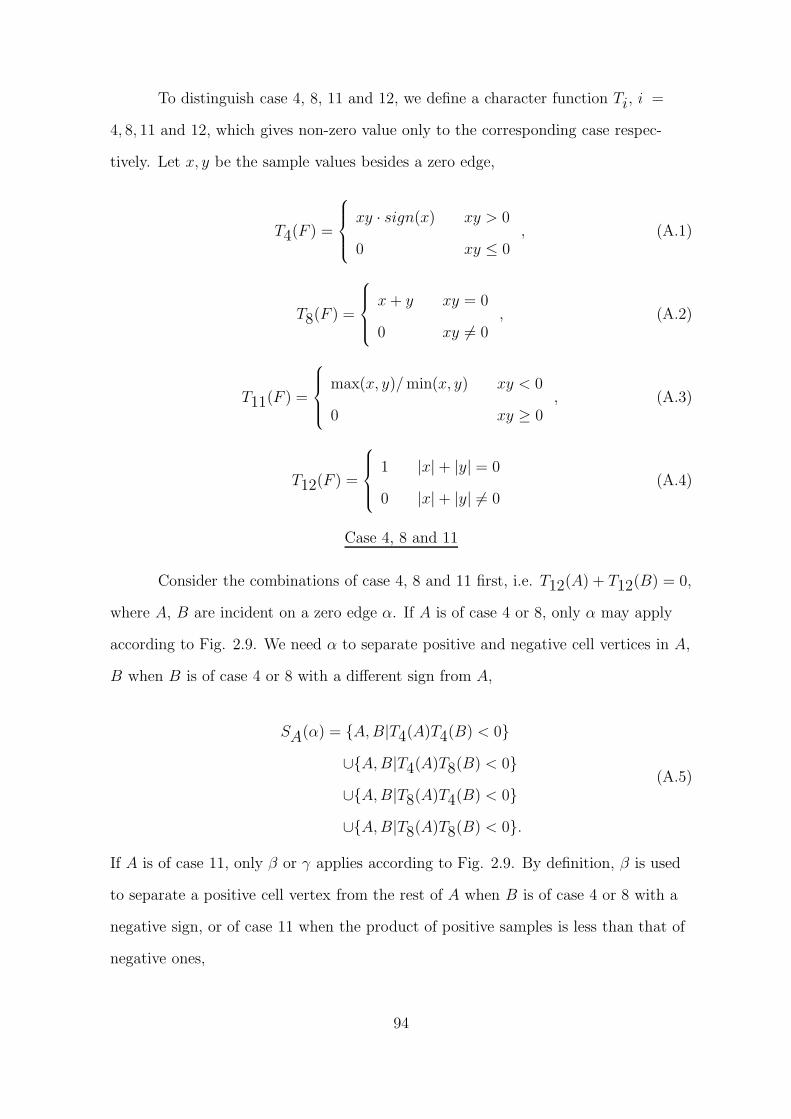
To distinguish case 4, 8, 11 and 12, we define a character function Ti, i =
4, 8, 11 and 12, which gives non-zero value only to the corresponding case respec-
tively. Let x, y be the sample values besides a zero edge,
T4(F ) =
xy · sign(x) xy > 0
0 xy ≤ 0, (A.1)
T8(F ) =
x+ y xy = 0
0 xy 6= 0, (A.2)
T11(F ) =
max(x, y)/min(x, y) xy < 0
0 xy ≥ 0, (A.3)
T12(F ) =
1 |x| + |y| = 0
0 |x| + |y| 6= 0(A.4)
Case 4, 8 and 11
Consider the combinations of case 4, 8 and 11 first, i.e. T12(A) + T12(B) = 0,
where A, B are incident on a zero edge α. If A is of case 4 or 8, only α may apply
according to Fig. 2.9. We need α to separate positive and negative cell vertices in A,
B when B is of case 4 or 8 with a different sign from A,
SA(α) = A,B|T4(A)T4(B) < 0
∪A,B|T4(A)T8(B) < 0
∪A,B|T8(A)T4(B) < 0
∪A,B|T8(A)T8(B) < 0.
(A.5)
If A is of case 11, only β or γ applies according to Fig. 2.9. By definition, β is used
to separate a positive cell vertex from the rest of A when B is of case 4 or 8 with a
negative sign, or of case 11 when the product of positive samples is less than that of
negative ones,
94

SA(β) = A,B|T11(A) 6= 0, T4(B) < 0
∪A,B|T11(A) 6= 0, T8(B) < 0
∪A,B|0 < T11(A)T11(B) < 1.
(A.6)
Similarly, γ is used to separate a negative cell vertex from the rest of A when B is
of case 4,8 with a positive sign, or of case 11 when the product of positive samples is
no less than that of negative ones,
SB(γ) = A,B|T11(A) 6= 0, T4(B) > 0
∪A,B|T11(A) 6= 0, T8(B) > 0
∪A,B|T11(A)T11(B) ≥ 1.
(A.7)
To get the results in Fig. 2.10, we enumerate all the combinations of case 4,
8, and 11 and solve SA(α), SA(β) and SA(γ) using equation (A.5), (A.6) and (A.7).
Case 12
Then consider the combinations with case 12, i.e T12(A)+T12(B) 6= 0. If only
B is of case 12, i.e. T12(A) = 0, T12(B) 6= 0, we search along the direction vertical
to α for the next cell face C that is not of case 12. We treat cell vertices besides zero
edges α, δ adjacent, to solve α, β, and γ similar to equation (A.5) ∼ (A.7). If A is
of case 4 or 8, only α or δ may apply according to Fig. 2.9. Either α or δ is chosen
to separate positive and negative cell vertices in A,C when C is of case 4 or 8 with a
different sign from A. Subdividing SA(α) into two parts and replacing B with C, we
have
S∗A(α) = A,C|T4(A)T4(C) < 0, |T4(A)| < |T4(C)|
∪A,C|T8(A)T8(C) < 0, |T8(A)| < |T8(C)|
∪A,C|T8(A)T4(C) < 0,
(A.8)
95

S∗C (δ) = A,C|T4(A)T4(C) < 0, |T4(A)| ≥ |T4(C)|
∪A,C|T8(A)T8(C) < 0, |T8(A)| ≥ |T8(C)|
∪A,C|T4(A)T8(C) < 0,
(A.9)
where we choose α when the absolute value of the product of sample values besides
the zero edge in A is less than that in C, or when A is of case 8 and C is of case 4.
If A is of case 11, S∗A(β) and S∗A(γ) can be directly derived by replacing B with C
in SA(β), SA(γ) of equation (A.6), (A.7) respectively. If A is of case 12, i.e. T12(A) 6=
0, we search in both directions vertical to α for the next two cell faces not of case 12.
Without loosing generality, let T12(B) + T12(D) = 0, SA(α) can be computed based
on Property 1 as SA(α) = SB(α).
To get the result in Fig. 2.11, we enumerate all the configurations with a cell
face of case 12, and solve S∗A(α) and S∗C(δ) using equation (A.6) ∼ (A.9).
96

APPENDIX B
PROOF OF THE THEOREM OF VERTEX DEGREE
97

Firstly, it is easy to verify the degree of a surface vertex that is not zero cell
vertex is two, since it is shared by two cell faces, in each of which one patch edge is
connected to the vertex. And the degree of surface vertex in Fig. 2.11 is either zero
or two.
Secondly, we show that the degree of surface vertex is at most two for the
cases with zero cell vertices in Fig. 2.7(a) and Fig. 2.10. In Fig. 2.7(a), the only
possibility for the degree of surface vertex to reach three is at zero cell vertices with
three adjacent cell faces. However, if one zero cell vertex connects to three patch
edges like case 5 or 9, it will cause a contradiction in which the cell vertices at two
sides of a patch edge are of the same sign. So the degree of surface vertex is at most
two in cases in Fig. 2.7(a). In Fig. 2.10, we only need to verify the degree of zero
cell vertices that possibly connect more than one patch edge is at most two. Such
zero cell vertices, called multi-edge vertices for convenience, exist in sub-case 4.d,
11.b, 11.c.1, 11.c.2, 8.e, 8.g and 8.h. From cases 2 and 7 in Fig. 2.7(a), a zero cell
vertex connects to no patch edge if its two adjacent cell vertices are of the same sign.
So a multi-edge vertex connects to no patch edge in its third adjacent cell face (not
displayed) in sub-cases 11.c.1, 11.c.2, 8.e or 8.g in Fig. 2.10. Since only two cell ver-
tices are not known in Fig. 2.10, we get the degree of the multi-edge vertex is two by
enumerating nine combinations of the two unknown cell vertices in the sub-cases 4.d,
11.b and 8.h. So the degree of surface vertex is at most two in cases in Fig. 2.10.
Finally we show that the degree of a zero cell vertex is not one. We only need
to check zero cell vertices that connect only one patch edge in Fig. 2.7(a) and Fig.
2.10, connect at least one patch edge in other adjacent cell faces. Such zero cell ver-
tex is called single-edge vertex for convenience. From case 5 and 9 of Fig. 2.7(a), a
zero cell vertex connects to only one patch edge on one cell face if its two adjacent
cell vertices are of different signs. Similarly it connects to at least one patch edge in
its other adjacent cell faces, if its third adjacent cell vertex (not displayed) is positive
or negative. If its third adjacent cell vertex is a zero cell vertex, only two other un-
98

known cell vertices (not displayed) that affect its degree are left. We get the degree
of a single-edge vertex is two by enumerating nine combinations of the two unknown
cell vertices. In Fig. 2.10, the degree of a zero cell vertex in sub-cases 4.c, 4.e, 11.e.1,
11.e.2 is two since its two adjacent cell vertices are of different signs. Since only two
unknown vertices (not displayed) are left in Fig. 2.10, by enumerating nine combina-
tions of the two unknown cell vertices, we get the degree of the single-edge vertex is
two in sub-case 4.d, 11.b, 11.d, 8.e, 8.g and 8.h.
In conclusion, the degree of surface vertex in one cell by the case rules of bi-
linear interpolation and zero edge is either zero or two.
99

APPENDIX C
COMPLEXITY OF ONLINE COMPUTING FOR SPHERICAL HARMONICS
COEFFICIENTS
100
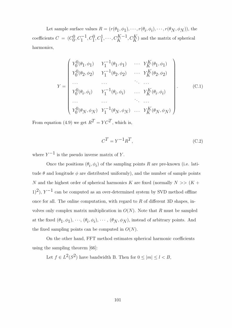
Let sample surface values R = (r(θ1, φ1), · · · , r(θi, φi), · · · , r(θN , φN )), the
coefficients C = (C00 , C
−11 , C0
1 , C11 , · · · , C
K−1K ,CKK ) and the matrix of spherical
harmonics,
Y =
Y 00 (θ1, φ1) Y−1
1 (θ1, φ1) · · · Y KK (θ1, φ1)
Y 00 (θ2, φ2) Y−1
1 (θ2, φ2) · · · Y KK (θ2, φ2)
. . . . . .. . . . . .
Y 00 (θi, φi) Y−1
1 (θi, φi) . . . Y KK (θi, φi)
. . . . . .. . . . . .
Y 00 (θN , φN ) Y−1
1 (θN , φN ) . . . Y KK (θN , φN )
. (C.1)
From equation (4.9) we get RT = Y CT , which is,
CT = Y−1RT , (C.2)
where Y−1 is the pseudo inverse matrix of Y .
Once the positions (θi, φi) of the sampling points R are pre-known (i.e. lati-
tude θ and longitude φ are distributed uniformly), and the number of sample points
N and the highest order of spherical harmonics K are fixed (normally N >> (K +
1)2), Y−1 can be computed as an over-determined system by SVD method offline
once for all. The online computation, with regard to R of different 3D shapes, in-
volves only complex matrix multiplication in O(N). Note that R must be sampled
at the fixed (θ1, φ1), · · ·, (θi, φi), · · · , (θN , φN ), instead of arbitrary points. And
the fixed sampling points can be computed in O(N).
On the other hand, FFT method estimates spherical harmonic coefficients
using the sampling theorem [66]:
Let f ∈ L2(S2) have bandwidth B. Then for 0 ≤ |m| ≤ l < B,
101

f(l,m) =
√2π
2B
2B−1∑
j=0
2B−1∑
k=0a(B)j f(θj, φk)e−imφkPml (cos θj), (C.3)
where Pml is the associate Legendre function, the sample points are chosen from the
equiangular grid: θj = π(2j + 1)/4B, φk = 2πk/2B, and the weights a(B)j play a
role analogous to the sin θ factor in the integrals.
In terms of online computation, FFT method involves multiplication and ad-
dition proportional to the number of sampling points N because all except the sam-
ple surface value f(θj, φk) in (C.3) can be computed offline.
In sum, the complexity online computation is approximated as O(N) for both
SVD and FFT methods.
102

APPENDIX D
COMPUTING 4D HYERSPHERICAL HARMONICS (HSH) COEFFICIENTS
103

The process to compute 4D HSH coefficients Cmλ,l is very similar to that of
coefficients Cml of 3D SH. We just outline the formulas. Let sample voxel values
R = (r(θ1, φ1, θ01), · · · , r(θi, φi, θ0i), · · · , r(θN , φN , θ0N )), the coefficients C =
(C00,0, C
01,0, C
−11,1 , C
01,1, C
11,1, · · · , C
K−1K,K ,CKK,K) and the matrix of spherical har-
monics,
Y =
Y 00,0(θ1, φ1, θ01) Y 0
1,0(θ1, φ1, θ01) · · · Y KK,K(θ1, φ1, θ01)
Y 00,0(θ2, φ2, θ02) Y 0
1,0(θ2, φ2, θ02) · · · Y KK,K(θ2, φ2, θ02)
. . . . . .. . . . . .
Y 00,0(θi, φi, θ0i) Y 0
1,0(θi, φi, θ0i) · · · Y KK,K(θi, φi, θ0i)
. . . . . .. . . . . .
Y 00,0(θN , φN , θ0N ) Y 0
1,0(θN , φN , θ0N ) · · · Y KK,K(θN , φN , θ0N )
.
(D.1)
From equation (5.11) we get RT = Y CT , which is,
CT = Y−1RT , (D.2)
where Y−1 is the pseudo inverse matrix of Y .
We sample (θi, φi, θ0i) uniformly over 4D unit sphere, with θi ∈ [0, π], φi ∈
[0, 2π], and θ0i ∈ [0, π]. Another way to sample (θi, φi, θ0i) is to convert voxels from
Cartesian coordinates to Polar coordinates directly using equation (5.5).
We use Mathematica function SphericalHarmonicY to compute 3D spheri-
cal harmonics, and get 4D hyperspherical harmonics using equation (5.7), (5.8) and
(5.9) [95].
For N sample points and the highest degree of HSH K, the size of matrix Y
is N × (K+1)(K+2)(2K+3)6 . Normally N >>
(K+1)(K+2)(2K+3)6 , we need to
compute Y−1 by singular value decomposition (SVD). For example, for a (θi, φi, θ0i)
grid of size 20×20×20 and K = 8, the size of Y is 8000×285. This step can be com-
104

pleted offline once for all hyperspherical functions, which is sampled at fixed position
(θi, φi, θ0i).
105

REFERENCES
[1] W. E. Lorensen and H. E. Cline, “Marching cubes: A high-resolution 3D sur-face construction algorithm,” in Proceedings of the 14th annual conference oncomputer graphics and interactive techniques, 1987, pp. 163–169.
[2] E. V. Chernyaev, “Marching cubes 33: Construction of topologically correct iso-surfaces,” CERN, Geneva, Switzerland, Tech. Rep. CN/95-17, 1995.
[3] “Spherical harmonic,” MathWorld. [Online]. Available: http://mathworld.wolfram.com/SphericalHarmonic.html
[4] J. Vesanto and E. Alhoniemi, “Clustering of the Self-Organizing Map,” IEEETransactions on Neural Networks, vol. 11, pp. 586–600, 2000.
[5] R. Osada, T. Funkhouser, B. Chazelle, and D. Dobkin, “Shape distributions,”ACM Transactions on Graphics, vol. 21, pp. 807–832, 2002.
[6] D. V. Vranic, “3D model retrieval,” Ph.D. dissertation, University of Leipzig,2004.
[7] M. Kazhdan, T. Funkhouser, and S. Rusinkiewicz, “Rotation invariant sphericalharmonic representation of 3D shape descriptors,” in Eurographics Symposiumon Geometry Processing(2003), 2003, pp. 156–165.
[8] E. Osuna, R. Freund, and F. Girosi, “Support vector machines:Training and applications,” Artificial Intelligence Laboratory, MassachusettsInstitute of Technology, Tech. Rep. AIM-1602, 1997. [Online]. Available:citeseer.ist.psu.edu/osuna97support.html
[9] G. M. Nielson and B. Hamann, “The asymptotic decider: Resolving the ambiguityin marching cubes,” in Proceedings of Visualization ’91, 1991, pp. 29–38.
[10] B. K. Nataranjan, “On generating topologically consistent isosurfaces fromuniform samples,” The Visual Computer, vol. 11, no. 1, pp. 52–62, 1994.
[11] S. V. Matveyev, “Approximation of isosurface in the marching cubes: Ambiguityproblem,” in IEEE Visualization, 1994, pp. 288–292.
[12] G. M. Nielson, “On marching cubes,” IEEE Transaction on Visualization andComputer Graphics, vol. 9, no. 3, pp. 283–297, 2003.
[13] A. Lopes and K. Brodlie, “Improving the robustness and accuracy of themarching cubes algorithm for isosurfacing,” IEEE Transaction on Visualizationand Computer Graphics, vol. 9, no. 1, pp. 16–29, 2003.
106

[14] H. Theisel, “Exact isosurfaces for marching cubes,” Computer Graphics Forum,vol. 21, no. 1, pp. 19–31, 2002.
[15] L. P. Kobbelt, M. Botsch, U. Schwanecke, and H.-P. Seidel, “Feature sensitivesurface extraction from volume data,” in ACM SIGGRAPH 2001, 2001, pp.57–66.
[16] T. Ju, F. Losasso, S. Schaefer, and J. Warren, “Dual contouring of hermitedata,” in 29th annual conference on Computer graphics and interactive tech-niques, 2002, pp. 339–346.
[17] R. Shekhar, E. Fayyad, R. Yagel, and J. F. Cornhill, “Octree-based decimationof marching cubes surfaces,” in IEEE Visualization 1996, 1996, pp. 335–342.
[18] R. Westermann, L. Kobbelt, and T. Ertl, “Real-time exploration of regularvolume data by adaptive reconstruction of iso-srufaces,” The Visual Computer,vol. 15, no. 2, pp. 100–111, 1999.
[19] J. Wilhelms and A. V. Gelder, “Octrees for faster isosurface generation,” ACMTransactions on Graphics, vol. 11, no. 3, pp. 201–227, 1992.
[20] C. Montani, R. Scateni, and R. Scopigno, “A modified lookup table for implicitdisambiguation of marching cubes,” The Visual Computer, vol. 10, no. 6, pp.353–355, 1994.
[21] ——, “Discretized marching cubes,” in Proceeding of the Visualization ’94.Congress, 1994, pp. 281–287.
[22] A. Cuno, C. Esperanca, A. Oliveira, and P. R. Cavalcanti, “Fast polygonizationof variational implicit surfaces,” in XVII Brazilian Symposium on ComputerGraphics and Image Processing, 2004, pp. 258–265.
[23] A. V. Gelder and J. Wilhelms, “Topological considerations in isosurface genera-tion,” ACM Transactions on Graphics, vol. 13, no. 4, pp. 337–375, 1994.
[24] J. Bloomenthal and K. Ferguson, “Polygonization of non-manifold implicitsurfaces,” in ACM SIGGRAPH 1995, 1995, pp. 309–316.
[25] A. Hubeli and M. Gross, “Multiresolution methods for nonmanifold models,”IEEE Transactions on Visualization and Computer Graphics, vol. 7, no. 3, pp.207–221, 2001.
[26] H.-C. Hege, M. Seebas, D. Stalling, and M. Zockler, “A generalized marchingcubes algorithm based on non-binary classifications,” Zuse Institute Berlin (ZIB),Tech. Rep. SC 97-05, 1997.
[27] S. Yamazaki, K. Kase, and K. Ikeuchi, “Non-manifold implicit surfaces based ondiscontinuous implicitization and polygonization,” in Geometric Modeling andProcessing - Theory and Applications, 2002, pp. 138–147.
107

[28] X. Han, C. Xu, and J. Prince, “A topology preserving level set method forgeometric deformable models,” IEEE Transactions on Pattern Analysis andMachine Intelligence, vol. 25, no. 6, pp. 755–768, June 2003.
[29] D. C. Banks and S. Linton, “Counting cases in marching cubes: Toward a genericalgorithm for producing substitopes,” in IEEE Visualization 2003, 2003, pp.51–58. [Online]. Available: http://www.dcs.st-and.ac.uk/research/publications/BL03.php
[30] “Eulerian circuit,” MathWorld. [Online]. Available: http://mathworld.wolfram.com/EulerianCircuit.html
[31] J. W. Tangelder and R. C. Veltkamp, “A survey of content based 3D shaperetrieval methods,” in Proceedings Shape Modeling International, 2004, pp.145–156.
[32] R. J. Campbell and P. J. Flynn, “A survey of free-form object representation andrecognition techniques,” Computer Vision and Image Understanding, vol. 81, pp.166–210, 2001.
[33] N. Iyer, K. Lou, S. Jayanti, K. Y., and K. Ramani, “Three dimensional shapesearching: State-of-the-art review and future trends,” Computer Aided Design,2004.
[34] M. Herbert, K. Ikeuchi, and H. Delingette, “A spherical representation forrecognition of free-form surfaces,” IEEE Transactions on Pattern Analysis andMachine Intelligence, vol. 17, pp. 681–690, 1995.
[35] J. Li, “Three dimensional shape modeling: Segmentation, reconstruction andregistration,” Ph.D. dissertation, Electrical Engineering, the University ofMichigan, 2002.
[36] D. Saupe and D. V. Vranic, “3D model retrieval with spherical harmonics andmoments,” in Proceedings of the DAGM 2001, B. Radig and S. Florczyk, Eds.,2001, pp. 392–397.
[37] D. V. Vranic, “An improvement of rotation invariant 3D shape descriptor basedon functions on concentric spheres,” in ICIP 2003, vol. 3, 2003, pp. 757–760.
[38] D.-Y. Chen, X.-P. Tian, Y.-T. Shen, and M. Ouhyoung, “On visual similaritybased 3D model retrieval,” in Eurographics Computer Graphics Forum, vol. 22,2003, pp. 223–233.
[39] X. Gu, S. J. Gortler, and H. Hoppe, “Geometry Images,” in Proceedings ofSIGGRAPH, 2002, pp. 355–361.
[40] H. Laga, H. Takahashi, and M. Nakajima, “Geometry image matching forsimilarity estimation of 3D shapes,” in Proceedings of the Computer GraphicsInternational (CGI’04), 2004, pp. 490–496.
108

[41] H.-s. Wong, K. K. Cheung, and H. H. Ip, “3D head model classification byevolutionary optimization of the Extended Gaussian Image representation,”Pattern Recognition, vol. 37, pp. 2307–2322, 2004.
[42] J. Corney, H. Rea, D. Clark, J. Pritchard, M. Breaks, and R. MacLeod, “Coarsefilters for shape matching,” IEEE Computer Graphics and Applications, vol. 22,no. 3, pp. 65–74, 2002.
[43] S. Biasotti, S. Marini, M. Mortara, and G. Patané, “An overview onproperties and efficacy of topological skeletons in shape modeling,” in SMI ’03:Proceedings of the Shape Modeling International 2003. Washington, DC, USA:IEEE Computer Society, 2003, p. 245.
[44] “Topology,” MathWorld. [Online]. Available: http://mathworld.wolfram.com/Topology.html
[45] S. Liu and J. Li, “Enumerating all the marching cubes cases withzero cell vertices,” SECS in Oakland University. [Online]. Available:http://www.secs.oakland.edu/∼sliu2/MC/mc.htm
[46] T. Lewiner, H. Lopes, A. W. Vieira, and G. Tavares, “Efficient implementation ofmarching cubes’ cases with topological guarantees,” Journal of Graphics Tools,vol. 8, no. 2, pp. 1–15, 2003.
[47] R. Malladi, J. A. Sethian, and B. C. Vemuri, “Shape modeling with frontpropagation: A level set approach,” IEEE Transactions on Pattern Analysis andMachine Intelligence, vol. 17, no. 2, pp. 158–175, Feb 1995.
[48] C. Baillard, C. Barillot, and P. Bouthemy, “Robust adaptive segmentation of 3Dmedical images with level sets,” INRIA, Tech. Rep. RR-4071, 2000.
[49] A. Dempster, N. Laird, and D. Rubin, “Maximum likelihood from incompletedata via the EM algorithm,” Journal of Royal Statistical Society, vol. 3, pp. 1–38,1976.
[50] A. Tsai, W. Wells, S. Warfield, and A. Willsky, “Level set methods in an EMframework for shape classification and estimation,” in MICCAI (1) 2004, 2004,pp. 1–9.
[51] P. Masson and W. Pieczynski, “SEM algorithm and unsupervised statisticalsegmentation of satellite images,” IEEE Transaction on Geoscience and RemoteSensing, vol. 31, no. 3, pp. 618–633, 1993.
[52] C. Ciofolo, C. Barillot, and P. Hellier, “Combining fuzzy logic and level setmethods for 3D MRI brain segmentation,” in IEEE International Symposium onBiomedical Imaging (ISBI), 2004, pp. 161–164.
[53] P. Lin, C.-X. Zeng, Y. Yang, and J.-W. Gu, “Statistical model based on levelset method for image segmentation,” in The Fourth International Conference onComputer and Information Technology, 2004, pp. 143–148.
109

[54] “Lung Image Database Consortium (LIDC) Materials,” National CancerInstitute. [Online]. Available: http://imaging.cancer.gov/reportsandpublications/ReportsandPresentations/LungImaging
[55] C.-C. Ho, P.-L. Lee, Y.-Y. Chuang, B.-Y. Chen, and M. Ouhyoung, “Cubicalmarching squares: Adaptive feature preserving surface extraction from volumedata,” in EUROGRAPHICS, vol. 24, 2005.
[56] M. Novotni and R. Klein, “A geometric approach to 3D object comparison,”in Proceedings of the 5th ACM SIGMM international workshop on Multimediainformation retrieval, 2003, pp. 39–45.
[57] D. V. Vranic, D. Saupe, and J. Richter, “Tools for 3D-object retrieval: Karhunen-Loeve transform and spherical harmonics,” in Proceedings of the IEEE 2001Workshop Multimedia Signal Processing, J.-L. Dugelay and K. Rose, Eds., 2001,pp. 293–298.
[58] S. Haker, S. Angenent, A. Tannenbaum, R. Kikinis, G. Sapiro, and M. Halle,“Conformal surface parameterization for texture mapping,” IEEE Transactionson Visualization and Computer Graphics, vol. 6, pp. 240–251, 2000.
[59] H. Hoppe, T. DeRose, and T. Duchamp, “Multiresolution analysis of arbitrarymeshes,” in Computer Graphics (SIGGRAPH’95 Proceedings), 1995, pp. 173–182.
[60] X. Gu and S. T. Yau, “Computing conformal structures of surfaces,” in Commu-nication of Information and Systems, vol. 2, 2002, pp. 121–146.
[61] C. Gotsman, X. Gu, and A. Sheffer, “Fundamentals of spherical parameterizationfor 3D meshes,” ACM Transactions on Graphics, vol. 22, pp. 358–363, 2003.
[62] T. Tasdizen and R. Whitaker, “Geometric surface processing via normal maps,”ACM Transactions on Graphics, vol. 22, no. 4, pp. 1012–1033, Oct. 2003.
[63] K. Ikeuchi and M. Hebert, “Spherical representations: from EGI to SAI,”Computer Science Department, Carnegie Mellon University, Tech. Rep. CMU-CS-95-197, 1995.
[64] E. Praun and H. Hoppe, “Spherical parameterization and remeshing,” inProceedings of ACM SIGGRAPH, 2003, pp. 340–349.
[65] R. B. Schudy and D. H. Ballard, “Towards an anatomical model of heartmotion as seen in 4-D cardiac ultrasound data,” in Proceedings of the 6th Con-ference on Computer Applications in Radiology and Computer-Aided Analysis ofRadiological Images, 1979.
[66] D. M. J. Healy, D. Rockmore, P. J. Kostelec, and S. S. B. More, “FFTs for the2-sphere - improvements and variations,” The Journal of Fourier Analysis andApplications, vol. 9, pp. 341–385, 2003.
110
[67] D. Zhang and M. Hebert, “Multi-scale classification of 3D objects,” RoboticsInstitute, Carnegie Mellon University, Tech. Rep. CMU-RI-TR-96-39, 1996.
[68] H. Hoppe, “Progressive meshes,” in SIGGRAPH 96, 1996, pp. 99–108.
[69] “3D Database,” Signal Analysis and Machine Perception Laboratory (SAMPL).[Online]. Available: http://sampl.eng.ohio-state.edu/∼sampl/data/3DDB/Models/index.htm
[70] P. Shilane, P. Min, M. Kazhdan, and T. Funkhouser, “Princeton ShapeBenchmark.” [Online]. Available: http://shape.cs.princeton.edu/benchmark/
[71] D. V. Vranic, “3D MODEL DATABASE.” [Online]. Available: http://merkur01.inf.uni-konstanz.de/CCCC/dbsel.html
[72] “The Stanford 3D Scanning Repository,” Stanford University ComputerGraphics Laboratory. [Online]. Available: http://www-graphics.stanford.edu/data/3Dscanrep/
[73] “SOM toolbox for Matlab,” SOM Toolbox team in CIS HELSINKIUNIVERSITY OF TECHNOLOGY. [Online]. Available: http://www.cis.hut.fi/projects/somtoolbox/
[74] M. M. Kazhdan, “Shape representations and algorithms for 3D model retrieval,”Ph.D. dissertation, The Department of Computer Science in Princeton University,2004.
[75] J. Huang, R. Yagel, V. Filippov, and Y. Kurzion, “An accurate method forvoxelizing polygon meshes,” in IEEE Symposium on Volume Visualization, 1998,pp. 119–126. [Online]. Available: citeseer.ist.psu.edu/article/huang98accurate.html
[76] M. W. Jones, “The production of volume data from triangular meshes usingvoxelisation,” Computer Graphics Forum, vol. 15, no. 5, pp. 311–318, 1996.
[77] W. J. Schroeder, W. E. Lorensen, and S. Linthicum, “Implicit modeling ofswept surfaces and volumes,” in VIS ’94: Proceedings of the conference onVisualization ’94. Los Alamitos, CA, USA: IEEE Computer Society Press, 1994,pp. 40–45.
[78] F. Dachille and A. Kaufman, “Incremental triangle voxelization,” inGraphics Interface 2000, May 2000, pp. 205–212. [Online]. Available:citeseer.ist.psu.edu/dachille00incremental.html
[79] F. S. Nooruddin and G. Turk, “Simplification and repair of polygonal models usingvolumetric techniques,” IEEE Transactions on Visualization and ComputerGraphics, vol. 9, no. 2, pp. 191–205, 2003.
[80] T. Funkhouser, P. Min, M. Kazhdan, J. Chen, A. Halderman, and D. Dobkin,“A search engine for 3D models,” ACM Transactions on Graphics, vol. 22, pp.83–105, 2003.
111

[81] M. Murata and S. Hashimoto, “Interactive environment for intuitive under-standing of 4d object and space,” in International Conference on MultimediaModeling, 2000, pp. 383–401.
[82] K. A. Mitchell and R. G. Littlejohn, “Derivation of planar three-body hyper-spherical harmonics from monopole harmonics,” Phys. Rev. A, vol. 56, no. 1, pp.83–99, Jul 1997.
[83] J. Avery, Hyperspherical Harmonics and Generalized Sturmians. Dordrecht,Netherlands: Kluwer Academic Publishers, 2000.
[84] A. Matheny and D. B. Goldgof, “The use of three- and four-dimensional surfaceharmonics for rigid and nonrigid shape recovery and representation,” IEEETrans. Pattern Anal. Mach. Intell., vol. 17, no. 10, pp. 967–981, 1995.
[85] A. V. Meremianin, “Multipole expansions in four-dimensional hypersphericalharmonics,” Journal of Physics A Mathematical General, vol. 39, pp. 3099–3112,Mar. 2006.
[86] M. Ouhyoung, D.-Y. Chen, and J.-S. Yeh, “NTU 3D model benchmark.”[Online]. Available: http://3d.csie.ntu.edu.tw/∼dynamic/benchmark/index.html
[87] B. E. Boser, I. Guyon, and V. Vapnik, “A training algorithm for optimal marginclassifiers,” in Computational Learning Theory, 1992, pp. 144–152. [Online].Available: citeseer.ist.psu.edu/boser92training.html
[88] V. N. Vapnik, The nature of statistical learning theory. New York, NY, USA:Springer-Verlag New York, Inc., 1995.
[89] S. Canu, Y. Grandvalet, V. Guigue, and A. Rakotomamonjy, “SVMand kernel methods Matlab toolbox,” Perception Systemes et Information,INSA de Rouen, Rouen, France, 2005. [Online]. Available: http://asi.insa-rouen.fr/∼arakotom/toolbox/index.html
[90] R. Kohavi and B. Becker, “UCI adult database,” also known as Census IncomeDatabase. [Online]. Available: http://mlearn.ics.uci.edu/MLSummary.html
[91] T. Joachims, “Learning to classify text using support vector machines,” Ph.D.dissertation, Cornell University, 2002.
[92] ——, Making large-Scale SVM Learning Practical. Advances in Kernel Methods- Support Vector Learning. MIT Press, 1999.
[93] ——, “SVMLight,” an implementation of Support Vector Machines (SVMs) inC. [Online]. Available: http://svmlight.joachims.org/
[94] M. Li, “Confidence-based classifier design and its applications,” Ph.D. disserta-tion, Oakland University, 2005.
[95] “Spherical harmonic,” Mathematica. [Online]. Available: http://functions.wolfram.com/HypergeometricFunctions/SphericalHarmonicYGeneral/
112

PUBLICATIONS
[1] Shaojun Liu, Jia Li, and Xiaojun Jing, ”Surface Construction using TricolorMarching Cubes,” in International Conference on Computer Graphics Theoryand Applications (GRAPP), 2006, pp. 319-324.
[2] Shaojun Liu and Jia Li, ”Genus-Zero Shape Classification Using Spherical Nor-mal Image,” in International Conference on Pattern Recognition (ICPR), 2006,pp. 126-129.
[3] Shaojun Liu and Jia Li, ”Automatic Medical Image Segmentation Using Gra-dient and Intensity Combined Level Set Method,” in IEEE International Con-ference of the Engineering in Medicine and Biology Society (EMBS), 2006, pp.3118-3121.
[4] Russel Deter, Jia Li, Wesley Lee, Shaojun Liu, Romeo Roberto, ”QuantitativeAssessment of Gestational Sac Shape: The Gestational Sac Shape Score,” ac-cepted to Ultrasound in Obstetrics and Gynecology, Jan. 2007.
[5] Shaojun Liu, Jia Li, ”Constructing Topologically Correct Isosurfaces by Zero-Crossing Marching Cubes”, submitted to Computers & Graphcs.
[6] Weihong Niu, Jia Li, Shaojun Liu, Timothy Talty, ”Intra-vehicle UWB Com-munication Testbed”, submitted to Military Communications Conference(MILCOM) 2007.
113