Your thesaurus codes are:10.11.1,10.19.2

ANDASTROPHYSICS

26.6.1997

3D self-consistent N-body barred models of the Milky Way

I. Stellar dynamics

R. Fux

Geneva Observatory, Ch. des Maillettes 51, CH-1290 Sauverny, Switzerland

Received April 23; accepted June 20, 1997

Abstract. Many 3DN -body barred models of the Galaxyextending beyond the Solar circle are realised by self-consistent evolution of various bar unstable axisymmet-ric models. The COBE/DIRBE K-band map, correctedfor extinction, is used to constrain the location of the ob-server in these models, assuming a constant mass-to-lightratio. The resulting view points in the best matching mod-els suggest that the inclination angle of the Galactic barrelative to the Sun-Galactic centre line is 28 ± 7.

Scaling the masses according to the observed radialvelocity dispersion of M giants in Baade’s Window, severalmodels reproduce satisfactorily the kinematics of disc andhalo stars in the Solar neighbourhood, as well as the disclocal surface density and scale parameters. These modelshave a face-on bar axis ratio b/a = 0.5 ± 0.1 and a barpattern speed ΩP = 50± 5 km/s/kpc, corresponding to acorotation radius of 4.3±0.5 kpc. The HI terminal velocityconstraints favour models with low disc mass fraction nearthe centre.

The large microlensing optical depths observed to-wards the Galactic bulge exclude models with a disc scaleheight hz <∼ 250 pc around R = 4 kpc, arguing for a con-stant thickness Galactic disc. The models also indicatethat a spiral arm starting at the near end of the bar cancontribute as much as 0.5× 10−6 to the optical depth inBaade’s Window. The mass-to-K luminosity ratio of theGalactic bulge is probably more than 0.7 (Solar units),and if the same ratio applies outside the bar region, thenthe Milky Way should have a maximum disc.

Key words: Galaxy: structure, kinematics and dynamics

1. Introduction

Recent results demonstrate that the Milky Way, as morethan 2/3 of disc galaxies and as suspected early on by

Send offprint requests to: R. Fux

de Vaucouleurs (1964) from a comparison of gas kinemat-ics towards the Galactic centre and in external galaxies,is a barred galaxy with the near side of the bar point-ing in the first Galactic quadrant. Evidence comes fromnear-IR surface photometry, discrete source counts, gasand stellar kinematics and gravitational microlensing (seeKuijken 1996 and Gerhard 1996 for reviews). The mostsuggestive data certainly are the COBE/DIRBE near-IRmaps of the Galactic bulge (Weiland et al. 1994; Dwek etal. 1995; Binney et al. 1996 for a non-parametric depro-jection). Estimates of the angle between the major axisof the bar and the Sun-Galactic centre line range from10 to 45 (e.g. Stanek et al. 1997).

Furthermore, the distribution of HII regions, youngstellar clusters, HI gas, CO clouds and dust betray theexistence of several Galactic spiral arms (Mihalas & Bin-ney 1981; Vallee 1995 and reference therein), and externalspiral galaxies of the same (Sbc) Hubble type as the MilkyWay have arm-interarm surface mass density ratios of or-der 2 out to at least 3 disc scale lengths from the centre(Rix & Zaritsky 1995). Hence the detailed structure of ourGalaxy clearly deviates from axisymmetry.

No self-consistent 3D dynamical barred model of theGalaxy including simultaneously stellar, gas and darkcomponents and extending beyond the Sun’s Galactocen-tric distance has been proposed yet. Existing stellar dy-namical models are either axisymmetric (Kuijken & Du-binski 1995; Durand et al. 1996) and/or restricted to asingle Galactic component (Zhao 1996 for the COBE-bar;Kent 1992 and Kuijken 1995 for an axisymmetric bulgemodel), and gas flow calculations always assume a rigidrotating bar potential (Mulder & Liem 1986; Wada 1994;Weiner & Sellwood 1996).

This paper presents the first step of a program aimingsuch a complete model. Many self-consistent pure stellardynamical barred models of the Milky Way are built fromN -body evolution of bar unstable axisymmetric models.This method, already applied to the Galaxy by Sellwood(1985; 1993), naturally takes into account the main dy-

namical processes acting in the evolution of real isolatedgalaxies, like those responsible for spontaneous bar forma-tion and self-sustained spiral structures (e.g. Zhang 1996).The N -body method also proves convenient to cope with adissipative gas component, as will be added to the modelsin the next step and described in a second paper.

The structure of this paper is as follow: in Sect. 2we describe the distinct initial conditions of the variouscomponents considered in the simulations. In Sect. 3, wegive some technical informations about the N -body in-tegration and present the time evolution of the initialmodels. In Sect. 4 we determine for each evolved modelthe best location of the observer (the Sun) according tothe COBE/DIRBE near-IR observations of the Galacticbulge. In Sect. 5 we fix the velocity scales of the models tomatch the observed stellar velocity dispersion in Baade’sWindow and discuss some of the resulting absolute modelproperties.

2. Initial conditions

Equilibrium or close to equilibrium axisymmetric phasespace density functions (DF) have been obtained for discgalaxies either by applying the strong Jeans theoremwhich states that the DF is an explicit function of at mostthree isolating independent integrals of motion (Kuijken& Dubinski 1995; Durand et al. 1996), or by solving thehydrodynamical Jeans equations for the velocity momentsunder some arbitrary closure conditions and assuming aGaussian velocity distribution (Hernquist 1993).

The first method has the advantage to provide ex-act solutions of the Boltzmann equation, but is in gen-eral (except for Stackel potentials) limited by the lack ofan analytical third integral: DFs depending only on thetwo classical integrals, i.e. the total energy and the an-gular momentum about the symmetry axis (z), alwayshave σ2

Rz = 0, unsuitable for substantially anisotropicspheroidal components, and σ2

zz = σ2RR, which in the Solar

neighbourhood is wrong for any evolved stellar population.Moreover, generating DFs with imposed mass densities re-quires the cumbersome inversion of the integral equationthat relates these two quantities (Kuijken 1995 and refer-ences therein).

The second method allows for a larger variety of veloc-ity ellipsoids, depending on the closure conditions, and isalso more adapted for specified mass distributions. It wastherefore retained here, with some modification regardingthe shape of the velocity distribution.

The initial models are described in standard astronom-ical units, assuming that the Galactocentric distance ofthe Sun is R = 8 kpc. These units will serve as referencein the evolved models until Sect. 5.

2.1. Mass distribution

The initial mass density ρ in our simulations includes threeaxisymmetric components.

The first one is an oblate stellar nucleus-spheroid (NS)inspired from the model of Sellwood & Sanders (1988):

ρNS(s) =MNS

4πa3eI∞·

(s/a)p

1 + (s/a)p−q, (1)

where

s2 ≡ R2 + z2/e2, (2)

I∞ =π

p− qcsc

[(p+ 3)π

p− q

], (3)

a is a knee radius, e the axis ratio and MNS the integratedmass. Setting p = −1.8 and q = −3.3, this mass densitybehaves as s−1.8 for s a, in agreement with near-IRobservations of the Galactic inner kpc (Becklin & Neuge-bauer 1968; Matsumoto et al. 1982) if a constant mass-to-light ratio is assumed, and as s−3.3 for s a, similarto the radial number density decrease of RR Lyrae stars(Preston et al. 1991) and of the globular clusters (Zinn1985). This component is therefore well suited to repre-sent the nuclear bulge and the stellar halo.

The second component is a double exponential stellardisc:

ρD(R, z) =MD

4πh2Rhz

· exp

[−R

hR−|z|

hz

], (4)

where hR, hz and MD are resp. the scale length, the scaleheight and the integrated mass. This component standshere for the Galactic old disc.

Finally an oblate exponential dark halo (DH) with thesame axis ratio e as the NS component is added to ensurea flat rotation curve at large radii:

ρDH(s) =MDH

8πb3eexp(−s/b), (5)

where b is the scale length and MDH the total dark mass.

2.2. Truncation and flattening

To minimise the number of particles outside the force gridand increase the particle statistics near the centre (at fixednumber of particles), we softly truncate each componentmultiplying its mass density by:

f(s) = tanh

[s−Rc

2δ

], (6)

where Rc is the truncation radius and δ the width overwhich f falls from 1 to 0. The densities thus vanish on thespheroidal surface s = Rc.

In all simulations we set Rc = 38 kpc, δ = 5 kpc ande = 0.5. The choice of e is realistic at least for the NS com-ponent and has the technical advantage over more spher-ical models to limit the z-extension of the force grid.

2.3. Choice of mass density parameters

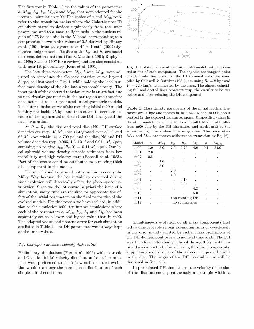
The first row in Table 1 lists the values of the parametersa, MNS, hR, hz, MD, b and MDH that were adopted for the“central” simulation m00. The choice of a and MNS resp.refer to the transition radius where the Galactic near-IRemissivity starts to deviate significantly from the innerpower law, and to a mass-to-light ratio in the nucleus re-gion of 0.75 Solar units in the K-band, corresponding to acompromise between the values of 0.5 derived by Binneyet al. (1991) from gas dynamics and 1 in Kent’s (1992) dy-namical bulge model. The disc scales hR and hz are basedon recent determinations (Fux & Martinet 1994; Ruphy etal. 1996; Sackett 1997 for a review) and are also consistentwith near-IR photometry (Kent et al. 1991).

The last three parameters MD, b and MDH were ad-justed to reproduce the Galactic rotation curve beyond3 kpc, as illustrated in Fig. 1, while holding the local sur-face mass density of the disc into a reasonable range. Theinner peak of the observed rotation curve is an artifact dueto non-circular gas motion in the bar region and thereforedoes not need to be reproduced in axisymmetric models.The outer rotation curve of the resulting initial m00 modelis fairly flat inside 25 kpc and then starts to decrease be-cause of the exponential decline of the DH density and themass truncation.

At R = R, the disc and total disc+NS+DH surfacedensities are resp. 48 M/pc2 (integrated over all z) and66 M/pc2 within |z| < 700 pc, and the disc, NS and DHvolume densities resp. 0.095, 1.3 ·10−3 and 0.014 M/pc3,summing up to give ρtot(R, 0) = 0.11 M/pc3. Our lo-cal spheroid volume density exceeds estimates from lowmetallicity and high velocity stars (Bahcall et al. 1983).Part of the excess could be attributed to a missing thickdisc component in the model.

The initial conditions need not to mimic precisely theMilky Way because the bar instability expected duringtime evolution will drastically affect the phase-space dis-tribution. Since we do not control a priori the issue of asimulation, many runs are required to appreciate the ef-fect of the initial parameters on the final properties of theevolved models. For this reason we have realised, in addi-tion to the simulation m00, ten further simulations whereeach of the parameters a, MNS, hR, hz and MD has beenseparately set to a lower and higher value than in m00.The adopted values and nomenclature for each simulationare listed in Table 1. The DH parameters were always keptat the same values.

2.4. Isotropic Gaussian velocity distribution

Preliminary simulations (Fux et al. 1996) with isotropicand Gaussian initial velocity distribution for each compo-nent were performed to check how self-consistent evolu-tion would rearrange the phase space distribution of suchsimple initial conditions.

Fig. 1. Rotation curve of the initial m00 model, with the con-tributions of each component. The squares are tangent pointcircular velocities based on the HI terminal velocities com-piled by Caldwell & Ostriker (1981), assuming R = 8 kpc andV = 220 km/s, as indicated by the cross. The almost coincid-ing full and dotted lines represent resp. the circular velocitiesbefore and after relaxing the DH component

Table 1. Mass density parameters of the initial models. Dis-tances are in kpc and masses in 1010 M. Model m00 is aboutcentred in the explored parameter space. Unspecified values inthe other models are similar to those in m00. Model m11 differfrom m00 only by the DH kinematics and model m12 by thesubsequent symmetry-free time integration. The parametersMNS and MDH are masses without the truncation by Eq. (6)

Model a MNS hR hz MD b MDH

m00 1.0 3.0 2.5 0.25 4.6 9.1 32.0m01 2.0 . . . . . .m02 0.5 . . . . . .m03 . 1.6 . . . . .m04 . 5.0 . . . . .m05 . . 2.0 . . . .m06 . . 4.0 . . . .m07 . . . 0.13 . . .m08 . . . 0.35 . . .m09 . . . . 4.2 . .m10 . . . . 5.0 . .

m11 . . non-rotating DH . .m12 . . no symmetries . .

Simultaneous evolution of all mass components firstled to unacceptable strong expanding rings of overdensityin the disc, mainly excited by radial mass oscillations ofthe DH damping out over a dynamical time scale. The DHwas therefore individually relaxed during 3 Gyr with im-posed axisymmetry before releasing the other components,suppressing indeed most of the subsequent perturbationsin the disc. The origin of the DH disequilibrium will bediscussed in Sect. 2.6.

In pre-relaxed DH simulations, the velocity dispersionof the disc becomes spontaneously anisotropic within a

few rotation periods, with a planar anisotropy compatible with first order epicycle theory (Binney & Tremaine1987) and ratios between the velocity dispersion compo-nents around R = R similar to those observed in theSolar neighbourhood for the old disc (see Fig. 2 in Fux etal. 1996 and Table 2). Hence isotropic initial kinematicsseems to suffice for the disc.

However, the kinematics of the NS never reaches theobserved radial velocity dispersion anisotropy of the localGalactic halo stars and instead sustains gravity throughtoo fast rotation, exceeding half the circular velocity (seeFig. 3c and Table 2). The mean rotation velocity can ofcourse be arbitrarily reduced by changing the sign of theazimuthal velocities of selected particles, but then the ro-tation velocity dispersion would increase and in turn de-viate from the local observations. Some radial anisotropyshould therefore appear already in the initial velocity dis-tribution of the NS component.

2.5. Anisotropic velocity dispersion

To achieve higher degree of radial velocity dispersionanisotropy in both the NS and the DH components, wehave solved the Jeans equations for more general closureconditions than just isotropy.

Following Bacon et al. (1983), we assume that the ve-locity ellipsoid points everywhere towards the Galacticcentre, i.e. σ2

rθ = 0 in spherical coordinates, with a freeanisotropy parameter β ≡ 1− σ2

θθ/σ2rr depending only on

r and of the form:

β(r) = β∞r√

r2 + r2

, (7)

where r is a transition radius and β∞ the asymptoticanisotropy at large r: β ∝ r for r r, and β = β∞ forr r. We also assume no other streaming motion thanrotation about the symmetry axis, i.e. vr = vθ = 0, andtake as boundary conditions σ2

rr = σ2θθ = 0 on the mass

truncation surface. The details of the numerical method,which can in fact also handle anisotropy parameter de-pending on θ, are presented in Fux (1997).

The solutions provide v2φ = vφ

2 + σ2φφ, leaving free

the relative contributions of organised and random veloc-ity in the φ direction. As a convenient choice, which en-sures isotropy near the centre and low rotation for r r,we set:

σ2φφ =

r2σ

2θθ + r2v2

φ

r2 + r2

, (8)

where r is the same parameter as in Eq. (7).The values of r and β∞ are restricted by the condition

v2φ ≥ 0 everywhere. In particular, on the truncation sur-

face of our initial mass models, this condition imposes anupper limit to β(r) in the range eRc < r < Rc dependingonly on the potential and its first derivatives (see Fig. 2).The resulting strongest constraint is β(eRc) < 0.65.

Table 2. Observed properties of the stellar halo (subdwarfs)and the old disc in the Solar neighbourhood. Σ is the total thindisc surface density (i.e. including also the young disc). Thevalues of the disc velocity dispersion are averages over z. Ref-erences are: (1) Majewski 1993, (2) Wielen 1977, (3) Sackett1997, (4) Kuijken & Gilmore 1989

Reference

Subdwarfs: σrr = σRR 131± 6 km/s 1σφφ 106± 6 km/s 1σθθ = σzz 85± 4 km/s 1vφ 37± 10 km/s 1

Old disc: σRR 48± 3 km/s 2σφφ 29± 2 km/s 2σzz 25± 2 km/s 2hz 300± 25 pc 3

Thin disc: Σ 48± 8 M/pc2 4

2.6. Dark halo disequilibrium and velocity distribution

Coming back to the DH radial oscillations, single relax-ation of DHs with Gaussian initial velocity distributionsbut variable radial velocity dispersion anisotropy basedon the technique outlined above (Sect. 2.5) indicate thatthe oscillations strengthen with the amount of anisotropy.From these experiments we inferred that the mass oscil-lations are in fact a consequence of the Gaussian tails inthe velocity distribution and the finite DH mass extent:a significant fraction of the DH particles, about 10% inthe isotropic case and increasing with radial anisotropy,have velocities which carry them outside the truncationsurface, unbalancing therefore the inner equilibrium.

To overcome this problem, the Gaussian velocity dis-tributions of the extended DH and NS components havebeen replaced by a bounded 3D distribution build uponstandard Beta distributions. This new “B3”-distributionhas four parameters, κ, λ, µ and ω (one per adjustablevelocity moment), and is described as a function of itsreduced variables ξ, η and ζ in Appendix A.

With the substitutions ξ ≡ vφ/v, η ≡ vr/ve andζ ≡ vθ/ve, the distribution is bounded in velocity spaceby a spheroidal surface with principal axes aligned withthe vφ, vr and vθ axes and of half-length v along vφ andve along vr and vθ. The boundary surface is not takenas a sphere because particles launched at a given spatialposition can afford higher velocities in the tangential di-rection than in the radial direction without escaping thesystem. Indeed, the boundary velocities v and ve can bequantified using the integrals of motion. If the velocity ofa particle is decomposed in an azimuthal component, vφ,and a meridional component, vm, then its energy writesE = 1

2 (v2m + L2

z/R2) + Φ, where Lz = R · vφ is the

angular momentum about the z-axis and Φ(R, z) is thegravitational potential. Assuming that the mass densityis bounded by an equipotential surface Φp and imposingvm = 0 when a particle reaches this surface (otherwise the

particle would cross the surface and escape), the conservation of energy and angular momentum yield the followingcondition for the confinement of the particle orbit insidethe system:

v2m +

R2p −R

2

R2p

v2φ < 2 [Φp − Φ(R, z)] , (9)

where Rp is the maximum cylindrical radius attained bythe particle. Thus:

ve =√

2(Φp − Φ), (10)

v =Rp√

R2p −R

2· ve, (11)

and v > ve.In our initial models, since the truncation surface of

the mass distribution is not an equipotential, we simplytake the maximum value of the potential on this sur-face, i.e. Φp ≡ Φ(Rc, 0), and set Rp = Rc. For the ini-tial m00 model, the resulting behaviour of ve and v inthe plane is shown in Fig. 3a. This will not prevent someparticles to escape but at least considerably reduces theDH disequilibrium and ensures well defined values of theboundary velocities everywhere inside the truncation sur-face.

If κ, λ ≤ 2, µ ≤ 3/2 or ω ≤ 1, the velocity distri-bution presents unphysical singularities on the boundaryspheroid which should in principle be avoided. In partic-ular, assuming vφ > 0 and substituting the requirementλ > 2 in Eq. (A10) yields:

vφ >−(v2

− v2φ) +

√(v2 − v

2φ)− 16v2

(v2 − 5v2

φ)

8v, (12)

which puts a lower limit on the mean rotation velocity,and thus further restricts the range of the parameter r.For the adopted mass truncation radius Rc and flatten-ing e, this condition unfortunately prevents NS modelswith mean rotation velocity below 100 km/s when ap-proaching R = Rc (see Fig. 3a). Therefore, to reproducethe observed rotation of the stellar halo in the Solar neigh-bourhood with Eq. (8), we decided to violate this condi-tion for the NS component and accept irregular velocitydistributions in a minor portion of the R−z plane. Simi-larly, the requirements µ > 3/2 and ω > 1 put constraintson the meridional components of the velocity dispersionwhich could be satisfied in all NS models, but not in thehot central part of the DHs.

The DH pre-relaxations have been maintained evenwith the adopted B3 velocity distribution to minimise anypersistent DH induced perturbations on the visible com-ponents. For these components, the Jeans equations weresolved using the total potential after relaxation, the noisein the potential being reduced by averaging the DH massdensity in time. The DH relaxation does not modify muchthe starting potential (see Fig. 1).

Fig. 2. Full line: anisotropy parameter β(r) of the NS compo-nent in all initial models. Dashed line: upper limit for positivev2φ on the mass truncation surface (in model m00)

2.7. Choice of velocity parameters

For the NS of simulation m00, the parameters r and β∞were adjusted to reproduce the observed rotation and ve-locity dispersion of the stellar halo in the Solar neigh-bourhood given in Table 2. The adopted parameters arer = 4.3 kpc and β∞ = 0.65, leading to the very closeto critical β(r) profile displayed in Fig. 2. The resultinginitial velocity moments of the NS are shown in Fig. 3a.

The reversal of the σ2rr versus σ2

φφ anisotropy at R ≈13 kpc is consistent with the kinematics of the blue hori-zontal branch field stars (Sommer-Larsen et al. 1994) andother halo stars (Beers & Sommer-Larsen 1995). The az-imuthal anisotropy at large radii could reflect the fact thatstars easier escape in the radial direction, and that σ2

rr

must vanish on the boundary of a finite and stationarysystem, whereas σ2

φφ can still be supported by low eccen-tricity orbits.

Figure 3b shows the NS kinematics in simulation m00shortly before the formation of the bar. Within R <∼ 14kpc, the NS looses a part of its radial velocity dispersionanisotropy and its rotation velocity raises. These changescertainly reflect the extreme nature of our initial condi-tions, i.e. forcing the radial anisotropy to its maximum.Nevertheless, the re-adjusted velocity moments still re-main much closer to the observations than those of sim-ulations started with isotropic NS velocity dispersion, asillustrated in Fig. 3c.

For the NS of the other simulations, we simply usethe same r and β∞ values than in simulation m00. Forthe DHs of simulations m00-m10, we set r = b andβ∞ = 0.1, compatible with the restriction of Eq. (12). Theinitial conditions for simulation m11 are identical withthose of m00, except that the DH has the same anisotropyβ(r) as the NS and no net rotation, i.e. σ2

φφ = v2φ in-

stead of Eq. (8), and hence also present an irregular outervφ-distribution. As justified by the preliminary simula-

Fig. 3. a Initial velocity dispersion and mean rotation veloc-ity of the NS component at z = 0 in simulation m00. Thetwo upper dotted lines give the meridional (ve) and azimuthal(v) escape velocities resulting from Eqs. (10) and (11), andthe lower dotted line the minimum admissible mean rotation(vφ,min) defined in Eq. (12) for regular velocity distribution.The circular velocity (Vc) is also represented. b Correspondingvelocity moments at t = 1200 Myr. c Velocity moments at thesame time in a simulation identical to m00 except that the NScomponent has isotropic initial velocity dispersion

tions, all discs have isotropic (β = 0) and Gaussian initialvelocity distribution, implying a velocity dispersion tightlyrelated to their scale heights.

3. Time evolution

The simulations m00-m11 were all done imposing 2-foldrotational symmetry about the z-axis and reflection sym-metry about the plane z = 0, hence reducing the nu-merical noise of the potential. For comparison, the initial

m00 model was also integrated without any symmetry,providing our last m12 simulation. Each simulation isrunned up to t = 5 Gyr, and ouputs of the particle phase-space coordinates were realised every 200 Myr, leaving325 evolved models to analyse.

The number of particles is fixed to 105 for the NS+disccomponents and 105 for the DH. The proportion of par-ticles in the NS and in the disc is such that the particlemasses are exactly the same for both components, andmay therefore change from one simulation to another: e.g.30262 NS particles and 69738 disc particles for m00.

3.1. N -body code

The initial models are integrated with the Particle-Meshcode described in Pfenniger & Friedli (1993).

The potential is computed on a cylindrical polar gridusing the fast Fourier transform technique in the φ and zdimensions, where the cells are equally spaced. The radialspacing of the cells is logarithmic with a linear core toavoid an accumulation point at the centre. The short rangeforces are softened by a variable homogeneous ellipsoidalkernel with semi-axes set to 1.1 times the respective celldimensions. The adopted grid has 25(R)× 24(φ)× 201(z)cells and extends up to 50 kpc in R and ±20 kpc in z,corresponding to a radial resolution of 40 pc at the centreand about 1.8 kpc at R.

The orbits are integrated using the standard leap-frogalgorithm with a time step of 0.1 Myr, representing a frac-tion of the crossing time of the central grid mesh in thesteep NS potential.

3.2. Model evolution

Figure 4 illustrates the evolution of our 13 simulations.They all lead to the formation of a bar, but not always onthe same time scale. Models with higher initial values ofToomre’s axisymmetric stability parameter Q in the re-gion of rising circular velocity need more time to developthe bar, in agreement with the work of Athanassoula &Sellwood (1986). This is the case for example when com-paring the simulations m07 and m08: the former startswith a much colder disc, i.e a lower value of Q, and indeedforms the bar more quickly.

The size of the bars clearly varies from one simulationto the other. However, one must keep in mind here thatthe evolved models can always be separately rescaled tolook more similar than they do in initial units, hence com-plicating an objective comparison. All bars finally flattenthe surrounding radial profile of the disc, the effect beingparticularly marked in simulation m03.

Some simulations obviously pass through a double barphase, like in m04t4400. The simulations also developtransient spiral arms, especially strong during the time ofbar formation. Such structures would be hard to achieveby other means than the N -body technique.

Fig. 4. Face-on surface density evolution in all runs, including 1/3 of all investigated models. The distances are in initial unitsand the contours are spaced with one magnitude interval. Rotation is clockwise. Note the induced asymmetries in run m12

Fig. 5. Pattern speed ΩP(t) of the bar in simulations m00,m04 and m08 (initial units). The pattern speed in the othersimulations roughly fall within the gap delimited by the m04and m08 solid lines

Figure 5 shows the bar pattern speed ΩP ≡dϑdt

(t) as afunction of time in three simulations. The azimuthal angleϑ of the bar major axis (in the inertial frame) is calculatedby diagonalising the Ixx, Iyy and Ixy components of themoment of inertia tensor of the NS+disc particles insideR < Re, where Re is the radius extremising the ratio of theinferred diagonal components. The noise level in the ΩP(t)curves depends on the bar strength and on the presenceof multiple rotating patterns.

After the first bar rotations, where the bar mayslow down by up to 15 km/s/kpc/Gyr, ΩP(t) is in gen-eral constant or slowly decreasing with a rate of a fewkm/s/kpc/Gyr. The lower rotation of the DH in simu-lation m11 does not influence the pattern speed of thebar: ΩP(t) in m11 is almost the same as in m00. Simula-tion m12 has a faster ΩP(t) decline than m00, probablyrelated to its noisier gravitational potential.

The presence of a dissipative gas component may alterthe bar evolution by speeding up its angular velocity andcausing its dissolution (Friedli & Benz 1993).

4. Location of the observer

The Diffuse Infrared Background Experiment (DIRBE)onboard the COBE satellite has mapped the full sky inten different bands, ranging from 1.25µm to 240µm, with aresolution of 0.7×0.7 and a field spacing of approximately0.32. The maps at 1.25 (J-band), 2.2 (K-band), 3.5 and4.9µm, dominated by integrated stellar light, clearly showan asymmetric boxy/peanut shaped bulge betraying theunderlying bar (Weiland et al. 1994).

The K-band map offers a good compromise betweenmaximum stellar emissivity, low extinction by dust andsmall relative contribution of zodiacal light. If a constantmass-to-light ratio is assumed throughout the Galaxy, it

should therefore provide a reliable tracer of the integratedmass distribution and thus put severe constraints on dy-namical models of the Milky Way.

This section presents a technique to find the view pointin an N -body galaxy from where the simulated panoramamost ressembles a fixed map, and applies the method toour models and a deredened version of the COBE K-banddata.

4.1. Reduction of the COBE K-band map

Even if extinction in the infrared is much less than in theoptical, it is still not negligeable (about 1.5 magnitude inK towards the Galactic centre).

Thus, following Arendt et al. (1994), the raw K-bandmap has been corrected for foreground dust extinction byfirst building a J−K color excess map under the assump-tion of constant intrinsic color, taken as the average colorin the region l < 30 and 10 ≤ b ≤ 15, and then trans-forming it into a K-band optical depth map using theredening law of Rieke & Lebofsky (1985). Such a correc-tion however is not valid for |b| <∼ 3 where a significantfraction of the integrated light is emitted along the dustscreen. Hence this low latitude region must be excludedin the fitting procedure.

Finally, the dust subtracted map has been symme-triesed in b and converted from its COBE Quadrilater-alised Spherical Cube representation to a cartesian gridmap in Galactic coordinates with ∆l = ∆b = 1 pixelsize, as shown in Fig. 6. This resolution ensures sufficientparticle statistics per pixel when computing model mapswithout bluring too much the data.

4.2. Fitting method

The position of the observer in the models is specified byits distance R in initial units from the “Galactic” centreand the scale free-angle ϕ between the line joining himselfto the centre and the major axis of the bar, with positiveϕ when the bar is leading the observer. We assume thatthe observer lies in the plane of symmetry, i.e. z = 0, andthat the visible components have a constant mass-to-lightratio ΥK in the K-band. Hence model maps of integratedlight will depend on R, ϕ and ΥK .

The flux per unit solid angle in a given pixel i is esti-mated from Monte Carlo integration:

Fi(R, ϕ,ΥK) = (ΥK∆Ω)−1Ni∑k=1

m

D2k + ε2

, (13)

where the sum ranges over all NS+disc particles insidepixel i, Ni is the total number of such particles, m themass per particle (identical for both visible components),Dk the distance of the kth particle relative to the observer,ε a softening parameter to reduce the statistical noise in-duced by the closest particles (ε2 = 0.1), and ∆Ω the solid

Fig. 6. Grid used for the data interpolation and the model fluxcalculation in the COBE-map fitting. The solid lines roughlydelimit the 100, 200, 300 and 400 pixels which in the modelshave the best particle statistics

angle sustained by the pixel. If b1 and b2 = b1 + ∆b arethe pixel limits in Galactic latitude, then:

∆Ω = ∆l(sin b2 − sin b1). (14)

The three parameters R, ϕ and ΥK are adjusted tothe COBE/DIRBE K-band data by minimising the meanquadratic relative residual between model and observedfluxes corrected for statistical noise, i.e. (see Appendix B):

R2(R, ϕ,ΥK) = (χ2 − ν)

Npix∑i=1

F i2

σ2i

−1

, (15)

where

χ2 =

Npix∑i=1

(Fi − F i )2

σ2i

, (16)

Npix is the number of pixel, ν = Npix − 3 the number ofdegree of freedom, F i the observed flux in pixel i, andσ2i the variance of Fi, whose best estimate reduces to (see

Appendix C):

σ2i = (ΥK∆Ω)−2

Ni∑k=1

(m

D2k + ε2

)2

. (17)

The data supply much more accurate fluxes than the mod-els, so that their errors may be neglected.

The standard χ2 minimisation method was abandonedbecause the χ2 strongly depends on the precision of theFi’s. In particular, the χ2 value will systematically in-crease with the number of particles available to computethe model maps (except for perfect models). Thus thefitted view points are biased towards regions where themodel maps are noisier, and the relative quality of differ-ent models cannot be judged from this indicator alone.Furthermore, the fact that the σ2

i ’s are only approxima-tions of the true variances causes an overestimation ofthe χ2 increasing with the uncertainties on the variances,which biases the solutions in the opposite way. This biaspersists even in R2 adjustments since R2 depends explic-itly on χ2. To reduce its effect, the σ2

i ’s have been averagedover the neighbouring pixels.

Only the bulge region |l| < 30 and 3 < b < 15enclosing the bar and with reliable dust correction, rep-resenting 720 pixels, is included in the fits. Moreover, toexclude pixels with low number of particles and to checkthe consistency of the fitted parameters with respect tothe selected l−b sub-region, the pixels are sorted by de-creasing Ni and only the most populated are retained,with Npix between 100 and 400. The typical l−b regionsselected this way are indicated in Fig. 6.

For each model, R2 is computed on a 2D grid in R andϕ with resolution ∆R = 0.1 kpc and ∆ϕ = 1. The pa-rameter ΥK does not require an extra dimension, since forfixed values of R and ϕ the optimum ΥK , which minimisesR2, can be calculated analytically as:

ΥK,min(R, ϕ) =

Npix∑i=1

F ′2iσ′2i− ν

Npix∑i=1

F ′iFi

σ′2i

−1

, (18)

where the primes indicate that the ΥK factor in Eqs. (13)and (17) is removed. The R2-grid is then smoothed byaveraging R2 over the 3 × 3 nearest grid points and theresulting minimum defines our best fit position of the ob-server.

4.3. Tests

The method has been tested with a simple mass modelconsisting in a triaxial multi-normal bulge for the bar andan axisymmetric Miyamoto-Nagai (1975) disc:

ρtest(x, y, z) =M1√

8π3σxσyσzexp

[−

1

2

(x2

σ2x

+y2

σ2y

+z2

σ2z

)]+b2MM2

4π

[aMR

2 + (aM + 3zb)(aM + zb)2

(R2 + (aM + zb)2)5/2z3b

], (19)

where R2 = x2 + y2, z2b = z2 + b2M, and with σx = 1.5,

σy = 0.8, σz = 0.4, aM = 5 and bM = 0.3. The Miyamoto-Nagai component is truncated at R = 15 and its masswithin this radius is 3M1.

COBE-like maps were computed for several input ob-serving points (Rin, ϕin) in the test model and 100 dis-tinct discrete realisations of this model with 105 particles,as in the NS+disc components of the dynamical models,were fitted to these maps by R2 minimisation, yieldingthe output observing points (Rout, ϕout). The statistics ofthe results is shown in Fig. 7.

For ϕin <∼ 40 and Rin <∼ 10, the systematic and sta-tistical errors on ϕout are at most +2 and 5 (except atsmall Rin for Npix = 100). For Npix ≥ 200, the statisticalerror on Rout is less than 4%, and Rout is underestimatedwith a systematic error increasing with Npix, which is in-timately connected with the χ2 bias already mentionedin Sect. 4.2: the additional pixels in the low flux regionhave the most uncertain σ2

i ’s and thus artificially enhancethe value of R2, as indicated in the top plots of Fig. 7.

Fig. 7. Test results of the R2 minimisation technique. Rin andϕin are the correct input coordinates of the observer and Rout

and ϕout the corresponding adjusted output parameters. Theleft and right columns are resp. for variable Rin and fixed ϕin,and for fixed Rin and variable ϕin. From top to bottom, basedon 100 experiments for each input position: the averages andstandard deviations of R2 at the minimum, Rout/Rin and ϕout.The full, long-dashed, short-dashed and dotted lines stand resp.for Npix = 100, 200, 300 and 400

4.4. Application

The R2 method has been applied to all dynamical models,noting ϕ and R the best fit parameters of the observerand R2

min the value of R2 at the minimum. An exampleof R2 topography is given in Fig. 8.

As a compromise between maximum exploitation ofthe data and minimum systematic errors on the fitted viewpoint parameters, we have privileged the case Npix = 300and sorted the models by increasing R2

min(300). Thismodel sequence was then truncated to include at least twomodels of each simulation, resulting in a sample of 68 mod-els with R2

min(300) ≤ 0.756% (hereafter our “A” sample).

Figure 9 shows the distribution of the adjusted anglesϕ for the models belonging to this sample as a function of

Fig. 8. R2 solution for the location of the observer in modelm08t3200, for Npix = 300. The R2 contours are spaced by0.5% and the cross indicates the position of the minimum. Theparameter ΥK has been substituted using Eq. (18)

Npix. Taking into account the uncertainties of the individ-ual angles, due to the moment of inertia method for deter-mining the absolute angular position of the bar major axisand to the intrinsic standard deviation of the R2 method,the 40 best models support an angle of ϕ = 28 ± 7

for the Galactic bar, with a possible overestimation by 2

according to the tests.

This result is consistent with the value of 20− 30

found recently by the OGLE team from the color magni-tude diagram of red clump giants in several fields acrossthe Galactic bulge (Stanek et al. 1997) and with the upperlimit of 30 set by the MACHO microlensing constraints(Gyuk 1996), and confirms the privileged 25 obtained bythe deprojection of the properly dust subtracted L-bandCOBE map (Binney et al. 1996; Bissantz et al. 1996).

The best models regarding the COBE constraints comefrom simulation m08, started with the thickest and hottestdisc. Indeed five of the six lowest residual models are fromthis simulation, with R2

min(300) ≈ 0.3−0.4%. For compar-ison, the initial m00 model has R2 ≥ 2.4% everywhere.Nevertheless, we note that model m06t4600 gives the bestCOBE-data match within the entire |l| < 90 region. Thismodel has a low disc scale height, close to the 204 pc de-rived by Kent et al. (1991) from the Spacelab IR Telescopedata with the assuption of constant hz.

Table 3 lists the results for a selection of A samplemodels (hereafter our “B” sample) which, in addition tothe COBE constraints, also best reproduce observationsin the Solar neighbourhood (see Sect. 5.1). The simula-tion m00 provide no acceptable model to enter this sub-sample.

The distance scale SR of the models now directly fol-lows by setting the best-fit Galactocentric distance of theobserver for Npix = 300 to R = 8 kpc. Figure 10 presentsthe NS+disc face-on configurations of some B samplemodels after such rescaling and the confrontation of thesemodels to the COBE data. The B sample models have aface-on surface density axis ratio b/a = 0.5 ± 0.1 for thecontours crossing the bar major axis at R = 2−3 kpc.

Fig. 9. Distribution of the best-fit position angle ϕ of the bar in the dynamical models. Dashed line: including all 68 modelsof the A sample; full line: including only the 40 lowest R2

min models of this sample

Table 3. Location of the observer in the final selection of models (B sample), as constrained by the COBE/DIRBE deredenedK-band map. The models are sorted by increasing R2

min(Npix = 300). The last two columns give the adopted distance (SR) andvelocity (SV ) scales based on the Npix = 300 solutions

Npix = 200 Npix = 300 Npix = 400

Model R ϕ[] R2

min [%] R ϕ[] R2

min [%] R ϕ[] R2

min [%] SR SVm08t4000 9.3 31 0.228 9.5 33 0.342 9.4 38 0.359 0.842 0.900m12t2000 8.2 23 0.319 8.2 23 0.409 8.2 23 0.337 0.976 0.939m06t4600 9.6 26 0.388 9.6 26 0.432 9.6 26 0.619 0.833 1.120m11t2000 8.1 27 0.365 9.0 34 0.467 8.2 28 0.526 0.889 0.964m08t3200 8.6 24 0.424 9.0 25 0.472 8.7 25 0.515 0.889 0.977m09t1600 8.5 26 0.341 8.5 26 0.586 8.5 26 0.828 0.941 0.991m02t2000 8.1 21 0.547 8.1 21 0.628 8.0 23 0.672 0.988 0.946m03t1000 7.5 22 0.599 9.5 29 0.641 8.0 21 0.728 0.842 1.056m12t1600 7.3 20 0.557 7.3 19 0.677 7.5 19 0.780 1.096 1.001m10t1400 7.4 19 0.580 8.1 22 0.709 7.4 15 0.730 0.988 0.916m04t3000 7.9 18 0.615 7.9 32 0.738 7.7 25 0.784 1.013 0.852m06t4800 8.0 26 0.675 8.0 25 0.747 9.3 9 0.650 1.000 1.137

Table 4. Several absolute properties of the rescaled B sample models. χ2loc: mean square residual between model and observed

local properties; σD, σS: local disc and NS velocity dispersions [km/s]; vφS: local NS rotation velocity [km/s]; hR, hz: disc scale

length [kpc] and local scale height [pc]; ΣD , ρS : local disc surface density [M/pc2] and NS volume density [10−3M/pc3];

V: local circular velocity [km/s]; ΩP, RL: pattern speed of the bar [km/s/kpc] and corotation radius [kpc]; ϕ: bar inclinationangle []; ΥK : mass-to-K band luminosity ratio [M/LK,]; τ0: microlensing optical depth towards Baade’s Window [10−6].Values in brackets include the DH lenses. The boldfaced models reasonably agree with most of the considered observations

Model χ2loc σDRRσ

Dφφσ

Dzz σSRR σSφφ σSzz vφ

S hR hz ΣD ρS V ΩP RL ϕ ΥK τ0m08t4000 2.98 43 28 21 106 117 78 51 2.7 363 47 0.9 195 36 5.5 33 0.60 1.53 (1.75)m12t2000 1.91 44 27 19 118 107 89 63 4.9 339 49 1.2 200 44 4.5 23 0.68 1.70 (2.12)m06t4600 5.59 36 26 17 135 129 95 41 4.0 232 58 1.3 230 54 3.9 26 0.59 1.45 (1.61)m11t2000 1.88 53 26 20 117 116 83 61 2.7 287 40 1.2 210 52 4.0 34 0.57 1.38 (1.48)

m08t3200 3.88 42 25 22 111 124 81 58 2.7 379 44 1.1 214 44 4.8 25 0.72 1.80 (1.97)m09t1600 3.61 38 24 18 124 121 84 61 4.4 259 50 1.2 212 55 3.9 26 0.73 2.19 (2.33)m02t2000 1.64 51 29 20 115 117 94 60 3.1 290 43 1.1 210 56 3.9 21 0.73 1.97 (2.07)m03t1000 2.47 41 30 18 129 125 93 44 4.9 271 45 0.6 216 58 3.9 29 0.53 1.54 (1.89)m12t1600 3.43 50 30 25 118 115 96 76 3.9 328 70 1.7 217 48 4.6 19 0.96 3.00 (3.13)m10t1400 1.82 54 28 18 119 111 91 64 5.1 295 47 1.2 198 44 4.9 22 0.70 1.97 (2.18)

m04t3000 3.40 36 24 19 111 106 84 50 3.0 285 39 1.5 200 48 4.3 32 0.72 2.03 (2.11)m06t4800 2.39 47 27 23 133 133 104 50 4.6 278 58 1.7 229 45 4.6 25 0.79 2.28 (2.46)

Fig. 10. Comparison of a selection of rescaled models with observations in the bar region. Left: face-on surface density of thevisible components; The symbol indicates the location of the observer and the crosses the positions of the Lagrangian pointsL1 and L2. Rotation is clockwise. Middle: COBE/DIRBE deredened K-band contours (full lines) and corresponding modelcontours (dashed lines). The b scale is dilated relative to l, hence amplifying the deviations. The region below the horizontal linewas excluded in the adjustments because of unreliable extinction correction. The spacing between the contours is 0.5 magnitudein both frames. Right: longitude-velocity diagram of the Galactic HI averaged over |b| < 1.25 and, superposed, the traces ofnon-self intersecting model x1-orbits (dashed lines); the innermost trace represents the cusped x1 orbit. The model m12t2000has been symmetrised in all frames. The HI data were kindly provided by H. Liszt and refer to Burton & Liszt (1978)

Fig. 10. continued

5. Model properties and discussion

Given the distance scale, there remains only one scaleleft in the models since the constraint of virial equi-librium links together the distance, velocity and massscales. We choose here to fix the velocity scale by re-quiring that the line-of-sight velocity dispersion of thecombined NS+disc components towards Baade’s Window(l, b) = (0.9,−3.9) equals 113 ± 6 km/s, as observed forlate-M giants (Sharples et al. 1990), leaving about 10%uncertainty on the absolute mass scale. The resulting ve-locity scales of the B sample models are listed in Table 3.

The complete scaling of the models allows now to de-rive several of their absolute properties, which are pre-sented and discussed in this section.

5.1. Local properties

The main local properties of the models, i.e. the proper-ties measured at the location of the observer, are givenin Table 4. These include the velocity dispersion of thedisc (σDRR, σ

Dφφ, σ

Dzz) and of the NS (σSRR, σ

Sφφσ

Szz), the NS

mean rotation velocity (vφS), the disc scale length (hR)

and scale height (hz), the disc surface density (ΣD ), theNS volume density (ρS ) and the circular velocity (V).

All quantities, except hR and V, are based on theparticles inside a sphere (for the NS) or a vertical cylinder(for the disc) centred on the Sun’s position, and hence arenot azimuthal averages. The disc scale length is an effec-tive exponential scale length derived from all disc particleswithin the annulus 0.7 < R/R < 1.2. The circular veloc-ity rests on the azimuthally symmetrised potential.

To quantify the ability of the models to reproduce local observations, Table 4 also gives the mean χ2 residualbetween the local model properties, from σDRR to ΣD andexcluding hR, and the corresponding observed values men-tioned in Table 2, weighting the contribution of the threedisc velocity dispersion components by 1/3 and the fourNS velocity moments by 1/4. Models from simulation m07have very high χ2

loc due to their small disc scale height,as well as unrealistic mass-to-light ratios and too low mi-crolensing optical depths in Baade’s Window (see Sect. 5.3and 5.4), and were therefore rejected.

Many models have disc kinematics consistent with ob-servations, and in particular correct ratios between thecomponents of the velocity dispersion. There appears aclear correlation between the vertical velocity dispersionof the disc and its scale height, as expected from self-gravitating isothermal sheets, although not directly de-pending on the disc surface density. A proper analysis ofthe disc vertical dynamics would of course require simula-tions with higher z-resolution. The disc velocity dispersionin model m06t4600 is lower than in m06t4800 because theobserver is located farther from the centre (in initial units)and the velocity dispersion decreases outwards.

The velocity dispersion of the NS components is ingeneral similar to that of the local Galactic halo stars, ex-cept that its radial anisotropy is insufficient. This differ-ence is probably linked to the initial model truncation atRc = 38 kpc, which limits the amount of radial anisotropyinside the models, and the flatness (e = 0.5) of the outermass distribution, which requires substantial support byazimuthal motion, either in systematic or random form. Itis however worthwhile to mention that the local subdwarfkinematics in Table 2 may be biased by selection effects.For example, kinematically selected samples have muchlarger radial anisotropy than samples selected by metal-licity criterions, the velocity dispersion in the latter beingeven consistent with meridional isotropy (Norris 1987).Moreover, the kinematics of the globular cluster systemshows no significant deviation from isotropy.

All models favour V < 220 km/s except those fromsimulation m06. These models have in fact increasing ro-tation curve from R/2 to R, so that our velocity scalingmainly based on the inner region leads to larger circularvelocities at R.

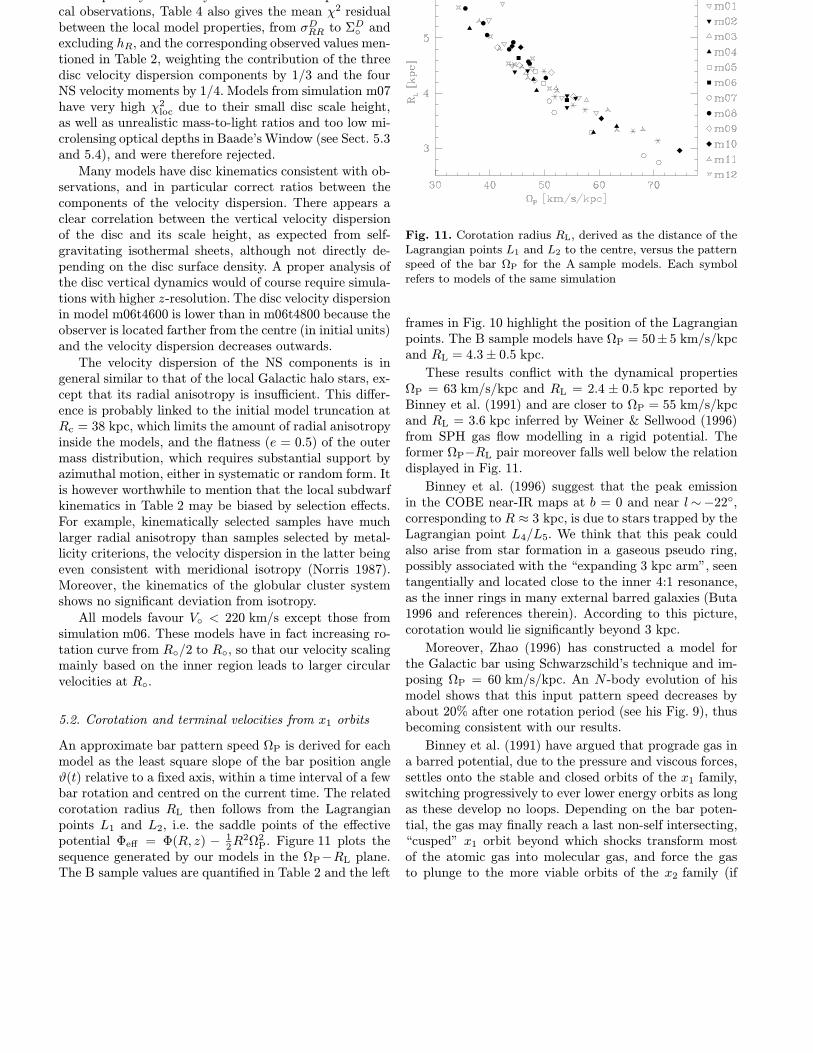
5.2. Corotation and terminal velocities from x1 orbits

An approximate bar pattern speed ΩP is derived for eachmodel as the least square slope of the bar position angleϑ(t) relative to a fixed axis, within a time interval of a fewbar rotation and centred on the current time. The relatedcorotation radius RL then follows from the Lagrangianpoints L1 and L2, i.e. the saddle points of the effectivepotential Φeff = Φ(R, z) − 1

2R2Ω2

P. Figure 11 plots thesequence generated by our models in the ΩP−RL plane.The B sample values are quantified in Table 2 and the left

Fig. 11. Corotation radius RL, derived as the distance of theLagrangian points L1 and L2 to the centre, versus the patternspeed of the bar ΩP for the A sample models. Each symbolrefers to models of the same simulation

frames in Fig. 10 highlight the position of the Lagrangianpoints. The B sample models have ΩP = 50± 5 km/s/kpcand RL = 4.3± 0.5 kpc.

These results conflict with the dynamical propertiesΩP = 63 km/s/kpc and RL = 2.4 ± 0.5 kpc reported byBinney et al. (1991) and are closer to ΩP = 55 km/s/kpcand RL = 3.6 kpc inferred by Weiner & Sellwood (1996)from SPH gas flow modelling in a rigid potential. Theformer ΩP−RL pair moreover falls well below the relationdisplayed in Fig. 11.

Binney et al. (1996) suggest that the peak emissionin the COBE near-IR maps at b = 0 and near l∼−22,corresponding to R ≈ 3 kpc, is due to stars trapped by theLagrangian point L4/L5. We think that this peak couldalso arise from star formation in a gaseous pseudo ring,possibly associated with the “expanding 3 kpc arm”, seentangentially and located close to the inner 4:1 resonance,as the inner rings in many external barred galaxies (Buta1996 and references therein). According to this picture,corotation would lie significantly beyond 3 kpc.

Moreover, Zhao (1996) has constructed a model forthe Galactic bar using Schwarzschild’s technique and im-posing ΩP = 60 km/s/kpc. An N -body evolution of hismodel shows that this input pattern speed decreases byabout 20% after one rotation period (see his Fig. 9), thusbecoming consistent with our results.

Binney et al. (1991) have argued that prograde gas ina barred potential, due to the pressure and viscous forces,settles onto the stable and closed orbits of the x1 family,switching progressively to ever lower energy orbits as longas these develop no loops. Depending on the bar poten-tial, the gas may finally reach a last non-self intersecting,“cusped” x1 orbit beyond which shocks transform mostof the atomic gas into molecular gas, and force the gasto plunge to the more viable orbits of the x2 family (if

an inner Lindblad resonance exists). Thus, atomic gas isexpected to move along non-self intersecting x1 orbits,providing the key for a model comparison with GalacticHI observations. In particular, the envelop defined by thetraces of such orbits in the longitude-velocity l−V diagramshould coincide with the observed HI terminal velocities.

Orbits of the x1 family have been computed in almostall our dynamical models, using the instantaneous frozenpotential. Figure 10 shows the comparison of severalmodel x1 traces versus HI contours in the l−V diagram.Some models reproduce fairly well the HI terminal ve-locity envelop. The best cases certainly are m04t3000 andm06t4600, which share the common property to arise fromsimulations with lower disc mass fraction in the bar re-gion: their disc to total mass ratio within s < 3 kpc isless than 0.45, where s is the variable defined in Eq. (2).Further cases from the B sample are m12t2000, m08t3200,m09t1600, m02t2000 and m06t4800. All these models, ex-cept m06t4800, occur shortly after the formation of thebar, when redistribution of angular momentum has notcompletely disturbed the initial exponential radial profileof the disc. In general, the presence of the bar tends tosteepen the azimuthally averaged inner radial profile ofthe disc, increasing the central disc surface density.

Most of the models also have x1 envelopes exceed-ing the observed terminal velocities, indicating that therecould be too much mass near the centre. Such an excesscould of course be reduced by increasing the angle ϕ, butthen the peaks of maximum and minimum velocity tracedby the cusped x1 orbit in the l−V diagram would alsobe shifted towards higher |l|. Reducing the velocity scalein general render the local disc kinematics less consistentwith observations.

Hence, if the Galactic gas really moves on non self-intersecting closed orbits, then the HI observations suggestthat our dynamical models could have too much mass inthe disc near the centre.

5.3. Mass-to-K luminosity ratio

In addition to the position of the observer, the COBE-fits in Sect. 4 also yield the K-band mass-to-light ratiosΥK of the models, without the contribution of the DHcomponent.

Taking ΥK, = 2.69 · 10−12 MW−1Hz (Wamsteker1981), the rescaled values for the B sample models rangefrom ΥK = 0.53 to 0.79 in Solar units, except for modelm12t1600 (see Table 2). The total NS+disc+DH mass ofthe B sample models within the spheroid s < 3 kpc is(2.6± 0.15)× 1010 M, with about 8% contribution fromthe DH component. This gives an average percentage bywhich ΥK is underestimated.

Modelling the gas dynamics of the barred galaxy M100(NGC4321), which has a Hubble type similar to the MilkyWay, Knapen et al. (1995) have inferred ΥK > 0.7 out-side its nuclear ring. Moreover, for stellar populations with

Fig. 12. Confrontation of a model with small hz/R to theCOBE data. The caption is similar to Fig. 10

near-IR emission dominated by late K and M giants, as forthe Galactic bulge (Arendt et al. 1994), similar mass-to-light ratios are expected (Worthey 1994). Such lower limitfor ΥK rules out some models, like those of simulation m07which all have ΥK < 0.4. The substantial microlensingoptical depths towards the Galactic bulge also argue for alarge value of ΥK , as discussed below in Sect. 5.4.

A noticeable difference between the COBE K-bandmap and the model maps in Fig. 10 is that the model con-tours are steeper in the low latitude and |l| >∼ 15 region,i.e. where the disc becomes dominant. Even if our correc-tion for extinction fails at b <∼ 3, the near-IR contoursin this region still remain very flat after more elaborateddust subtraction of the COBE data (Spergel et al. 1997)and hence the difference is probably real. Several reasonsmay lead to this departure.

First, the Galactic disc scale height may be lower bya factor ∼ 2 in the inner Galaxy than in the Solar neigh-bourhood, as deduced by Kent et al. (1991) from theSpacelab IR Telescope data and by Binney et al. (1996)from the deprojection of the COBE L-band map. At con-stant surface density, discs with smaller scale height aremore concentrated towards the plane and should there-fore contribute more to the low latitude near-IR emission.Our models, started with radially constant disc thickness,do not present such large disc scale height gradient out-side the bar region. But models from simulation m07 (seeFig. 12), with the thinnest disc, indeed have flatter l−bcontours than models from m08. The variable scale heightalternative however is not supported by observations in ex-ternal late-type spiral galaxies (de Grijs & van der Kruit1996 and reference therein).

Second, discs with more foreground mass between thebulge and the observer will also enhance the low lati-tude integrated light. This is the case for the m06 models(Fig. 10). At fixed total disc mass, because of the higherinitial disc scale length, these models have higher disc sur-

Fig. 13. a Dependence of the microlensing optical depths τ0 (without DH contribution) towards Baade’s Window on thecorotation radius RL, which is a reasonable indicator of the radial extension of the bar, and on the bar inclination angle ϕ,for the A sample models. The encircled points indicate models with prominent spiral structures. b Relation between τ0 and themass-to-light ratio ΥK for the same models. The symbols are as in Fig. 11

face density in the outer region, including the first few kpcbelow R. Increasing simply the disc mass is less efficientbecause the inner disc, mixing with the NS componentduring the bar instability, will also contribute more to thebulge emission.

Finally, the assumption ΥK = const. may not holdclose to the Galactic plane because of near-IR emissionfrom interstellar matter, or recent star formation. In thelatter case, red supergiants, too young for having diffusedas far above the plane as the old disc population, couldsignificantly contribute to the K-emission and reduce ΥK

at low Galactic latitude. However our COBE-adjustmentsshould not be affected by such a ΥK gradient since theregion |b| < 3 was excluded. Alternatively, the IR mass-to-light ratio could also be lower in the Galactic disc thanin the bulge, as found by Verdes-Montenegro et al. (1995)for NGC7217 in the I-band.

In the next section, we will argue for the massive discpossibility and against a variable disc scale height.

5.4. Bulge microlensing

The microlensing optical depths τ towards the galacticbulge provide a serious direct probe of the mass distribu-tion inside the Solar circle.

The first results obtained by the OGLE and MACHOexperiments favour surprisingly large optical depths: thereported values are at least (3.3± 1.2)× 10−6 for 9 bulgestars essentially located in Baade’s Window (Udalski et al.1994), and (3.9+1.8

−1.2)×10−6 for 13 clump giants with meanGalactic coordinates l = 2.55 and b = −3.64 (Alcocket al. 1997), whereas axisymmetric models predict valuesless than 10−6 (Evans 1994 and references therein). The

contribution of bulge lenses may however significantly in-crease the model predictions if the bulge is an elongatedbar seen nearly end-on (Evans 1994, Kiraga & Paczynsky1994, Zhao et al. 1996, Zhao & Mao 1996).

We have computed the model microlensing opticaldepths towards Baade’s Window, averaged over all sourcesalong the line-of-sight, from the following Monte Carloversion of Eq. (5) given by Kiraga & Paczynski (1994):

τβs =4πG

∆Ωc2

[∑Ds

∑Dd<Ds

(md

Dd−md

Ds

)D2βs

s

][∑Ds

D2βss

]−1

(20)

where the outer sums involve all source particles withina solid angle ∆Ω of the selected direction and the innersum all lens particles in the same solid angle between thespecified source and the observer, the symbols Ds and Dd

referring resp. to the source and lens distances relative tothe observer, andmd to the mass of the lens particles. G isthe gravitational constant, c the speed of light and βs theparameter introduced by Kiraga & Paczynski (1994) todescribe the detection probability of the sources: βs = 0if the sources are detectable whatever their distance, likeclump giant stars, and βs ≈ −1 for main sequence stars(Bissantz et al. 1996 and references therein).

Optical depths are calculated with and without includ-ing DH lenses. Table 4 gives some results for βs = 0. Theoptical depths for other values of βs are almost propor-tional to τ0: in particular, we find τ−1 ≈

23τ0, both with

or without DH lenses. The DH contributes roughly 9%to the total optical depth. In the mean direction of theAlcock et al. (1997) fields, τ0 is on the average 15% higherthan in Baade’s Window, in agreement with the abovereported observations.

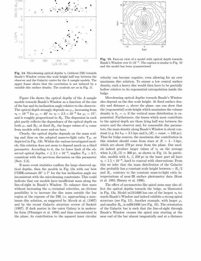
Fig. 14. Microlensing optical depths τ0 (without DH) towardsBaade’s Window versus disc scale height half way between theobserver and the Galactic centre for the A sample models. Theupper frame shows that the correlation is not induced by avariable disc surface density. The symbols are as in Fig. 11

Figure 13a shows the optical depths of the A samplemodels towards Baade’s Window as a function of the sizeof the bar and its inclination angle relative to the observer.The optical depth strongly depends on ϕ, increasing fromτ0 ∼ 10−6 for ϕ = 40 to τ0 ∼ 2.5× 10−6 for ϕ = 15,and is roughly proportional to RL. The dispersion in eachplot partly reflects the dependence of the optical depth onboth ϕ and RL: at fixed RL, the larger values of τ0 comefrom models with more end-on bars.

Clearly, the optical depths depends on the mass scal-ing and thus on the adopted mass-to-light ratio ΥK , asdepicted in Fig. 13b. Within the various investigated mod-els, this relation does not seem to depend much on a thirdparameter. According to it, the 1σ lower limit of the ob-served optical depths, τ >∼ 2.1× 10−6, implies ΥK > 0.7,consistent with the previous discussion on this parameter(Sect. 5.3).

If more event statistics confirm the large observed op-tical depths, then the models in Fig. 13a with our bestCOBE-estimate 28 ± 7 for the bar inclination angle areinconsistent with the microlensing constraints. This couldindicate that our models have insufficient mass along theline-of-sight in Baade’s Window. To enhance that masswithout increasing the x1-terminal velocities, an obviouspossibility is to increase the disc mass outside the barregion at the expense of the DH, i.e. approaching a max-imum disc solution, as suggested by Alcock at al. (1997)and by the recent Galactic structure review of Sackett(1997). If dark matter in the outer Galaxy is in molecu-lar form (Pfenniger et al. 1994) and thus concentrated inthe plane, its contribution to the squared inner circular

Fig. 15. Face-on view of a model with optical depth towardsBaade’s Window over 3×10−6. The caption is similar to Fig. 10and the model has been symmetriesed

velocity can become negative, even allowing for an overmaximum disc solution. To ensure a low central surfacedensity, such a heavy disc would then have to be partiallyhollow relative to its exponential extrapolation inside thebulge.

Microlensing optical depths towards Baade’s Windowalso depend on the disc scale height. At fixed surface den-sity and distance z1 above the plane, one can show thatthe (exponential) scale height which maximises the volumedensity is hz = z1 if the vertical mass distribution is ex-ponential. Furthermore, the lenses which most contributeto the optical depth are those lying half way between thesource and the observer and, for reasonable disc parame-ters, the mass density along Baade’s Window is about con-stant (e.g. for hR = 3.5 kpc and hz(R) = const. = 240 pc).Thus for bulge sources, the maximum disc contribution inthis window should come from stars at R = 4−5 kpc,which are about 270 pc away from the plane. Our mod-els indeed produce larger values of τ0 on the averagewhen hz(R/2) ≈ 300 pc, as shown in Fig. 14. In partic-ular, models with hz <∼ 250 pc in the inner part all haveτ0 < 1.5× 10−6, hard to conceal with observations. Fromthis we infer that the mass distribution of the Galacticdisc probably has a constant scale height between ∼ R/2and R, contrary to the constant mass-to-light ratio in-terpretations of near-IR surface photometry data (Kentet al. 1991; Binney et al. 1996).

The effect of asymmetries like spiral arms may also af-fect the optical depths towards the bulge, as illustratedin Fig. 13a. Model m12t1600 has one of the largest τ0 to-wards Baade’s Window and indeed exhibits a strong spiralstructure (see Fig. 15). Another example, with larger ϕand smaller RL, is m09t1600 (see Fig. 10). The orientationof the Galactic bar is such that the line-of-sight throughBaade’s Window crosses the spiral arm starting at thenear end of the bar almost tangentially and at a distance

Fig. 16a-d. Galactocentric radial kinematical properties of the model m08t3200. In all plots, the dashed, dotted and full linesstand resp. for disc, NS and disc+NS particles. a Radial velocity dispersion and mean velocity within |b| < 5 based on particlesinterior to the Solar circle. The points with error bars are derived from the te Lintel Hekkert et al. (1991) catalogue of doublepeaked OH/IR stars. b Projected radial velocity dispersion along the bar minor axis (l = 0). The data are from: (1) Sharples etal. 1990; (2) Terndrup published by Rich 1996; (3) Tyson & Rich 1991; (4) Rodgers 1977. c Projected radial velocity momentsalong an axis through the Galactic centre and inclined by 55 relative to the minor axis, and the corresponding Blum et al. (1995)M giant observations. The angle α is measured with respect to l = b = 0 and has the same sign as l. d Radial velocity dispersionin Baade’s Window as a function of the distance d from the observer, with the K giant data of Lewis & Freeman (1989). Thelower plot also represents the square root of the relative mass distribution per solid angle along the line-of-sight (arbitrary units)

where microlensing should be very efficient. The gain inoptical depth is of order 0.5× 10−6.

5.5. Inner kinematics

It is beyond the scope of this paper to study the de-tailed kinematics of all the dynamical models. Instead, wepresent here the case of a single model, m08t3200, which isin fair agreement with almost all explored constraints. InFigs. 16a-d, several kinematical predictions of this modelare compared to stellar observations.

The agreement between the longitudinal kinematics ofthe model disc and that of the OH/IR stars (Fig. 16a)is very convincing. The model particles outside the So-lar circle were not taken into account as the data con-tain only very few OH/IR stars at |l| > 90. No ve-locity moment has been derived from the data within|l| < 10 because in this region the radial velocity disper-sion depends non-negligibly on the galactic latitude andthe te Lintel Hekkert et al. (1991) OH/IR stars severelysuffer from undersampling at b <∼ 2.

The minor axis velocity dispersion of the model(Fig. 16b) is different for the NS and disc components.The observed kinematics are best traced by the NS com-ponent near the centre and by the disc component at largeGalactic latitude. In the Blum et al. (1995) fields, the kine-matics of these components are more similar (Fig. 16c).

The velocity dispersion in Baade’s Window as a func-tion of the distance from the observer is close to that ob-served for K giants (Fig. 16d), except near the tangentpoint. However, the projected velocity dispersion of thesestars is obviously less than the 113 km/s of the M gi-ants which was used to scale the model. Furthermore, thedistance distribution of the foreground model particles isroughly proportional to d 2, whereas the distribution of theK giants seems nearly linear with d (Sadler et al. 1996),suggesting that the latter may be biased towards the nearstars. This difference between model and observations ishardly due to a variable Galactic disc scale height. One canindeed show that, within 3−4 kpc from the observer, thesimulated line-of-sight mass distribution towards Baade’sWindow in a realistic analytical double exponential disc is

Table 5. Comparison of model m08t3200 versus K giant pro-jected radial kinematics in off axis bulge fields. Boldfaced, italicand roman velocities refer resp. to disc, NS and disc+NS par-ticles. The mean velocities are Galactocentric. The referencesfor the observations are Harding 1996, Minniti 1996a, Minniti1996b and Minniti et al. 1992

Observations Modell[] b[] [Fe/H] σr vr σr vr

-10.0 -10.0 > −1 67± 6 −82± 8 72 -81< −1 107 ± 6 −37± 8 120 -41

all – – 110 -719.9 -7.6 > −1 70± 7 56± 10 70 92

< −1 91± 13 −18± 18 117 40all – – 99 66

8.0 7.0 > −1 72± 4 66± 5 77 68< −1 109± 10 −7± 14 121 36

all – – 100 5412.0 3.0 – – – 75 111

– – – 124 45all 68± 6 77± 9 93 96

very similar for a radially constant or a linearly increasinghz if the face-on surface density profile is kept the same.

Table 5 reviews some off-axis K giant observations andgive the corresponding model predictions. The velocitymoments of the model disc component resemble those ofthe giants with [Fe/H]> −1. The l−b proper motion dis-persions of the model in Baade’s Window are (σµl , σµb) =(3.15, 2.38) m′′/yr for the disc, (2.96, 2.81) m′′/yr for theNS and (3.08, 2.57) m′′/yr for both visible componentstogether, whereas the observed values for K giants are(3.2± 0.1, 2.8± 0.1) m′′/yr (Spaenhauer et al. 1992).

6. Conclusion

We have built many self-consistent 3D dynamical barredmodels of the Milky Way extending beyond R = R byN -body integration of various bar unstable axisymmetricmodels. The models, extracted from the simulations at afrequency of 200 Myr, include 3 components: a nucleus-spheroid standing for the Galactic inner bulge and stellarhalo, a disc mainly representing the Galactic old disc anda non-dissipative dark halo. The comparison of the mod-els with observational constraints leads to the followingconsiderations.

1) The spatial location of the observer in each model isconstrained by the COBE/DIRBE K-band map correctedfor extinction by dust, assuming a constant mass-to-lightratio ΥK for the luminous mass components. The resultsfor the best matching models, with mean quadratic resid-uals between model and data fluxes down to 0.3%, suggestthat the angle between the l = b = 0 line and the majoraxis of the Galactic bar is 28 ± 7.

2) Scaling the models such as the distance of the ob-server to the centre is R = 8 kpc and the projected radialvelocity dispersion towards Baade’s Window 113 km/s, as

observed for M giants, absolute model properties are derived. A dozen of models reproduce fairly well both theCOBE-data and observations in the Solar Neighbourhood,although with a rather low radial versus azimuthal veloc-ity dispersion anisotropy of the spheroid components.

3) The bars in these models have a face-on axis ratiob/a = 0.5±0.1 and a pattern speed ΩP = 50±5 km/s/kpc,placing the corotation at 4.3 ± 0.5 kpc. Models with adisc mass fraction below 0.45 within 3 kpc from the cen-tre produce envelops of non self-intersecting x1-orbits inthe l−V diagram which better agree with the observed HIterminal velocities.

4) The microlensing optical depths of the models to-wards the bulge strongly depends on the bar inclinationangle ϕ, increasing from τ0 ∼ 10−6 for ϕ = 40 toτ0 ∼ 2.5 × 10−6 for ϕ = 15 towards Baade’s Window,whereas observations rather support values over 3× 10−6.We find that a spiral arm starting at the near end of thebar can increase the optical depths by 0.5×10−6 and thusreduce the gap between model and observed values.

5) All models with a disc scale height hz ≤ 250 pc halfway between the observer and the Galactic centre haveτ0 < 1.5 × 10−6, arguing against an inwards decreasingdisc scale height. This result is also in agreement with theconstant hz observed in late-type spirals.

6) The models predict a mass-to-K luminosity ratioΥK = 0.6−0.8 in Solar units. Values near the upper limitare consistent with the mass-to-light ratio estimated forM100 (NGC4321), a galaxy similar to the Milky Way, andfavour microlensing optical depths closer to the observedvalues. There is indeed an obvious but tight correlationbetween τ0 and ΥK , according to which τ0 >∼ 2 × 10−6

implies ΥK > 0.7.

7) Most models predict too low surface brightness rel-ative to the COBE-data in the region |l| <∼ 15 dominatedby the disc. Beside an improbable lower disc scale height inthe inner Galaxy, or a variable mass-to-light ratio, this dis-crepancy could indicate that the Galactic disc outside thebar region is more massive than assumed in the models,favouring large microlensing optical depths and arguingfor a maximum disc Milky Way.

8) The disc radial kinematics of the models resemblesthe observed kinematics of K giants with [Fe/H] > −1 inthe outer bulge.

As reasonable models regarding most observationalconstraints, we would recommend the models m08t3200and m04t3000.

Acknowledgements. I would like to thank L. Martinet and

D. Pfenniger for many enlightening discussions and for criti-

cal reading of the paper, as well as J. Sellwood for refering this

paper and D. Pfenniger for providing its efficient N-body code.

This work has been partially supported by the Swiss National

Science Foundation.

Appendix A: a non Gaussian bounded 3D distribution

A convenient 3D distribution with non-zero probabilityover a finite volume, i.e. avoiding the tails of the multi-normal distribution, is given by:

B3(ξ, η, ζ) =[2κ+λ−1B(κ, λ)B(1

2 , µ)B(12 , ω)

]−1·

(1+ξ)κ−2(1−ξ)λ−2(1− η2

1−ξ2 )µ−32 (1− ζ2

1−ξ2−η2 )ω−1

if ξ2 + η2 + ζ2 ≤ 1

0 otherwise,

(A1)

where B is the Beta function, and κ, λ, µ and ω are fourparameters. In the reduced variables ξ, η and ζ, this dis-tribution is bounded by a sphere of radius 1 on which, aslong as κ, λ > 2, µ > 3/2 and ω > 1, it continuously van-ishes. If κ = λ = 2, µ = 3/2 and ω = 1, the distributionis homogeneous inside the boundary sphere and smallervalues of these parameters produce singularities on it.

The first and second moments are:

η = ζ = (ξ − ξ)η = (ξ − ξ)ζ = ηζ = 0, (A2)

ξ =κ− λ

κ+ λ, (A3)

σ2ξξ ≡ (ξ − ξ)2 = 4

κλ

(κ+ λ)2(κ+ λ+ 1), (A4)

σ2ηη ≡ η2 =

4

2µ+ 1

κλ

(κ+ λ)(κ+ λ+ 1), (A5)

σ2ζζ ≡ ζ2 = σ2

ηη ·2µ

2ω + 1. (A6)

Depending on κ and λ, the distribution is skewed in ξ, themaximum of probability lying at:

ξmax =κ− λ

κ+ λ− 4. (A7)

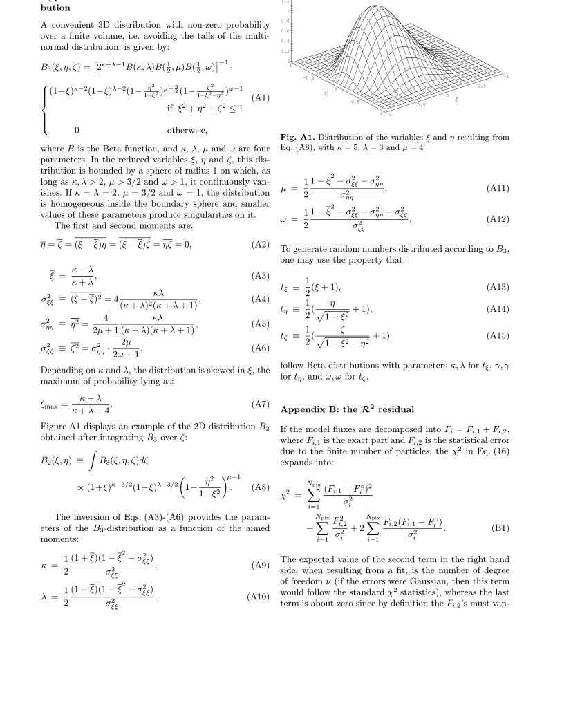
Figure A1 displays an example of the 2D distribution B2

obtained after integrating B3 over ζ:

B2(ξ, η) ≡

∫B3(ξ, η, ζ)dζ

∝ (1+ξ)κ−3/2(1−ξ)λ−3/2

(1−

η2

1−ξ2

)µ−1

. (A8)

The inversion of Eqs. (A3)-(A6) provides the param-eters of the B3-distribution as a function of the aimedmoments:

κ =1

2

(1 + ξ)(1− ξ2− σ2

ξξ)

σ2ξξ

, (A9)

λ =1

2

(1− ξ)(1− ξ2− σ2

ξξ)

σ2ξξ

, (A10)

-1

-0.5

0

0.5

1

-1

-0.5

0

0.5

1

0

0.2

0.4

0.6

0.8

1

1.2

Fig. A1. Distribution of the variables ξ and η resulting fromEq. (A8), with κ = 5, λ = 3 and µ = 4

µ =1

2

1− ξ2− σ2

ξξ − σ2ηη

σ2ηη

, (A11)

ω =1

2

1− ξ2− σ2

ξξ − σ2ηη − σ

2ζζ

σ2ζζ

. (A12)

To generate random numbers distributed according to B3,one may use the property that:

tξ ≡1

2(ξ + 1), (A13)

tη ≡1

2(

η√1− ξ2

+ 1), (A14)

tζ ≡1

2(

ζ√1− ξ2 − η2

+ 1) (A15)

follow Beta distributions with parameters κ, λ for tξ, γ, γfor tη, and ω, ω for tζ .

Appendix B: the R2 residual

If the model fluxes are decomposed into Fi = Fi,1 + Fi,2,where Fi,1 is the exact part and Fi,2 is the statistical errordue to the finite number of particles, the χ2 in Eq. (16)expands into:

χ2 =

Npix∑i=1

(Fi,1 − F i )2

σ2i

+

Npix∑i=1

F 2i,2

σ2i

+ 2

Npix∑i=1

Fi,2(Fi,1 − F i )

σ2i

. (B1)

The expected value of the second term in the right handside, when resulting from a fit, is the number of degreeof freedom ν (if the errors were Gaussian, then this termwould follow the standard χ2 statistics), whereas the lastterm is about zero since by definition the Fi,2’s must van-

ish on the average. With these simplifications, the bestestimate of the function:

R2 ≡

Npix∑i=1

1

σ2i /F

i

2

−1Npix∑i=1

[(Fi,1 − F i )/F i ]2

σ2i /F

i

2 , (B2)

i.e. the quadratic relative residuals between the Fi,1’s andthe F i ’s averaged over pixels and weighted by the inverseof the relative variance, indeed reduces to Eq. (15).

Appendix C: the variance of the model fluxes

The model flux in a given pixel is of the form:

F (D) =N∑k=1

f(Dk), (C1)

where N is the total number of particles in the pixel, theDk’s are the distances of the particles relative to the ob-server and D ≡ (D1, . . . , DN ). Noting resp. P (N) andp(D) the distributions of N and of the distances, the twofirst moments of F are:

Fn ≡∞∑N=0

P (N)·

∫ ∞0

dD1p(D1). . .

∫ ∞0

dDNp(DN )F (D)n

=

N · f n = 1

N f2 + (N f)2 n = 2,(C2)

where

N =∞∑N=0

NP (N), (C3)

fn =

∫ ∞0

p(D)f(D)ndD n = 1, 2. (C4)

The result for n = 2 in Eq. (C2) requires the assump-tion that the first and second moments of P are identical,which is true for Poisson statistics. Hence the variance ofF becomes:

σ2(F ) = F 2 − F2

= N · f2 ≈N∑k=1

f(Dk)2. (C5)

References

Alcock C., Allsman R.A., Alves D. et al. 1997, ApJ 479, 119Arendt R.G., Berriman G.B., Boggess N. et al. 1994, ApJ 425,

L85Athanassoula E., Sellwood J.A. 1986, MNRAS 221, 213Bacon R., Simien F., Monnet G. 1983, A&A 128, 405Bahcall J.N., Schmidt M., Soneira R.M. 1983, ApJ 265, 730Becklin E.E., Neugebauer G. 1968, ApJ 151, 145Beers T.C., Sommer-Larsen J. 1995, ApJS 96, 175Binney J., Gerhard O., Spergel D. 1996, preprint astro-

ph/9609066, submitted to MNRAS

Binney J., Gerhard O.E., Stark A.A., Bally J., Uchida K.I.1991, MNRAS 252, 210

Binney J., Tremaine S. 1987. In: Ostriker J.P. (Ed.) GalacticDynamics. New Jersey, Princeton Univ. Press, p. 120

Bissantz N., Englmaier P., Binney J., Gerhard O. 1996,preprint astro-ph/9612026, submitted to MNRAS

Blum R.D., Carr J.S., Sellgren K., Terndrup D.M. 1995, ApJ449, 623

Burton W.B., Liszt H.S. 1978, ApJ 225, 815Buta R. 1996. In: Buta R., Crocker D.A., Elmegreen B.G.

(eds.) Proc. IAU Coll. 157, Barred Galaxies. ASP Conf.Ser. 91, p. 11

Caldwell J.A.R., Ostriker J.P. 1981, ApJ 251, 61de Grijs R., van der Kruit P.C. 1996, A&AS 117, 19de Vaucouleurs G. 1964. In: Kerr F.J., Rodgers A.W. (eds.)

Proc. IAU-URSI Symp. 20, The Galaxy and the MagellanicClouds. Canberra, Aust. Acad. Sci., p. 88

Durand S., Dejonghe H., Acker A. 1996, A&A 310, 97Dwek E., Arendt R.G., Hauser M.G. et al. 1995, ApJ 445, 716Evans N.W. 1994, ApJ 437, L31Friedli D., Benz W. 1993, A&A 268, 65Fux R. 1997, PhD thesis, Geneva UniversityFux R., Martinet L. 1994, A&A 287, L21Fux R., Martinet L., Pfenniger D. 1996. In: Blitz L., Teuben P.

(eds.) Proc. IAU Symp. 169, Unsolved problems of theMilky Way. Dordrecht, Kluwer, p. 125

Gerhard O. 1996. In: Blitz L., Teuben P. (eds.) Proc. IAUSymp. 169, Unsolved problems of the Milky Way. Dor-drecht, Kluwer, p. 79

Gyuk G. 1996, preprint astro-ph/9607134Harding P. 1996. In: Morrison H., Sarajedini A. (eds.) Forma-

tion of the Galactic halo inside and out. ASP Conf. Ser. 92,p. 151

Hernquist L. 1993, ApJS 86, 389Kent S.M. 1992, ApJ 387, 181Kent S.M., Dame T.M., Fazio G. 1991, ApJ 378, 131Kiraga M., Paczynsky B. 1994, ApJ 430, L101Knapen J.H., Beckman J.E., Heller C.H., Shlosman I., De Jong

R.S. 1995, ApJ 454, 623Kuijken K. 1995, ApJ 446, 194Kuijken K. 1996. In: Buta R., Crocker D.A., Elmegreen B.G.

(eds.) Proc. IAU Coll. 157, Barred Galaxies. ASP Conf. Ser.91, p. 504

Kuijken K., Dubinski J. 1995, MNRAS 277, 1341Kuijken K., Gilmore G. 1989, MNRAS 239, 605Lewis J.R., Freeman K.C. 1989, AJ 97, 139Majewski S.R. 1993, ARA&A 31, 575Matsumoto T., Hayakawa S., Koizumi H. et al. 1982. In:

Riegler G., Blandford R. (eds.) The Galactic Center. NewYork: AIP, p. 48

Mihalas D., Binney J., 1981. In: Galactic astronomy. San Fran-cisco, Freeman Company, p. 525

Minniti D. 1996a, AJ 112, 590Minniti D. 1996b, ApJ 459, 579Minniti D., White S.D.M., Olszewski E.W., Hill J.M. 1992,

ApJ 393, L47Miyamoto M., Nagai R. 1975, Publ. Astron. Soc. Japan 27, 533Mulder W.A., Liem B.T. 1986, A&A 157, 148Norris J. 1987. In: Gilmore G., Carswell B. (eds) The Galaxy.

Dordrecht, Reidel, p. 297Pfenniger D., Combes F., Martinet L. 1994, A&A 285, 79

Pfenniger D., Friedli D. 1993, A&A 270, 561Preston G.W., Shectman S.A., Beers T.C. 1991, ApJ 375, 121Rich R.M. 1996. In: Morrison H., Sarajedini A. (eds.) Forma-

tion of the Galactic halo inside and out. ASP Conf. Ser. 92,p. 24

Rieke G.H., Lebofsky M.J. 1985, ApJ 288, 618Rix H.W., Zaritsky D. 1995, ApJ 447, 82Rodgers A.W. 1977, ApJ 212, 117Ruphy S., Robin A.C., Epchtein N. et al. 1996, A&A 313, 21Sackett P.D. 1997, preprint astro-ph/9608164, accepted by ApJSadler E.M., Rich R.M., Terndrup D.M. 1996, AJ 112, 171Sellwood J.A. 1985, MNRAS 217, 127Sellwood J.A. 1993. In: Holt S.S., Verter F. (eds) Back to the

Galaxy. New York, AIP, p. 133Sellwood J.A., Sanders R.H. 1988, MNRAS 233, 611Sharples R., Walker A., Cropper M. 1990, MNRAS 246, 54Sommer-Larsen J., Flynn C., Christensen P.R. 1994, MNRAS

271, 94Spaenhauer A., Jones B.F., Whitford A.E. 1992, AJ 103, 297Spergel D.N., Malhotra S., Blitz L. 1997, in preparationStanek K.Z., Udalski A., Szymanski M. et al. 1997, ApJ 477,

163te Lintel Hekkert P., Caswell J.L., Habing H.J., Haynes R.F.,

Norris R.P. 1991, A&AS 90, 327Tyson N.D., Rich R.M. 1991, ApJ 367, 547Udalski A., Szymanski M., Stanek K.Z. et al. 1994, Acta As-

tron. 44, 165Vallee J.P. 1995, ApJ 454, 119Verdes-Montenegro L., Bosma A., Athanassoula E. 1995, A&A

300, 65Wada K., Taniguchi Y., Habe A., Hasegawa T. 1994, ApJ 437,

L123Wamsteker W. 1981, A&A 97, 329Weiland J.L., Arendt R.G., Berriman G.B. et al. 1994, ApJ

425, L81Weiner B.J., Sellwood J.A. 1996. In: Blitz L., Teuben P. (eds.)

Proc. IAU Symp. 169, Unsolved problems of the Milky Way.Dordrecht, Kluwer, p. 145

Wielen R. 1977, A&A 60, 263Worthey G. 1994, ApJS 95, 107Zhang X. 1996, ApJ 457, 125Zhao H.S. 1996, MNRAS 283, 149Zhao H.S., Mao S. 1996, MNRAS 283, 1197Zhao H.S., Rich R.M., Spergel N.D. 1996, MNRAS 282, 175Zinn R. 1985, ApJ 293, 424

This article was processed by the author using Springer-VerlagLATEX A&A style file L-AA version 3.