3d fe simulations of resistance spot welding - diva portal915628/fulltext01.pdf · 3d fe...
TRANSCRIPT

IN ,DEGREE PROJECT ENGINEERING MECHANICS 120 CREDITSSECOND CYCLE
, STOCKHOLM SWEDEN 2016
3D FE Simulations of ResistanceSpot Welding
DAVID LÖVEBORN
KTH ROYAL INSTITUTE OF TECHNOLOGY
SCHOOL OF ENGINEERING SCIENCES

© Swerea KIMAB
3D FE Simulations of Resistance Spot Welding
David Löveborn
Report number [KIMAB-2016-108]
Box 7047, 164 40 Kista, Sweden + 46 8 440 48 00, www.swereakimab.se
Abstract
Resistance spot welding (RSW) is the
dominant joining technology in the
automotive industry. This is due to its low
costs and high efficiency. Other advantages
with RSW is the high ability for automation,
low consumption of energy, lack of need for
added materials and low degree of pollution,
no expensive equipment or education of
personal compared to arc welding and laser
welding. A modern automobile contains
approximately 4000 resistance spot welds,
which is why it is of great interest to be able
to predict the properties of the resistance spot
welds. The most important measurement
used to ensure the quality of the weld is the
nugget size, as it correlates to the welds
mechanical strength. This is usually
measured by destructive testing, and the most
common method is the coach peel test. This
test is performed by manually peeling the
specimen and then measuring the largest and
smallest nugget diameter. It is also possible
to perform non-destructive testing on
resistance spot welds with both ultrasonic-
and x-ray tests, however none of these
methods have the same accuracy as the
destructive methods and they are
cumbersome to use in large-scale. To
improve the efficiency and lower the cost for
the optimization of the welding parameters,
simulation tools have been developed. There
are both 2D- and 3D-simulation software to
model the RSW process. When the spot
welds are simulated with 2D or 2D axis-
symmetry, the number of elements is lower
compared to a full 3D model, which reduces
the computation times. The disadvantages
with the 2D model are the inabilities to
model misalignments or other asymmetrical
geometries. In contrast, the 3D-simulations
are not limited by these factors, and they are
also capable of modeling the shunt effects
occurring when a weld is placed close to a
previous weld.
The aims of this thesis was to evaluate such a
3D-simulation software, Sorpas 3D, and its
potential to be used in industrial process
planning, and to assess the software’s
usefulness for both simple and more complex
cases.
The results from this work show a good
correspondence between the simulations and
the physical tests. However, in order to
achieve these results a number of
modifications in the material properties were
required. Another critical limitation in the
software is that no expulsion criterion is
implemented. Considering the possibility that
the problems can be solved with a number of
updates in the software, Sorpas 3D can be a
useful tool in the process planning industry in
order to decrease process times and material
costs and improve the weld quality in the
future.

Box 7047, 164 40 Kista, Sweden + 46 8 440 48 00, www.swereakimab.se
Sammanfattning Punktsvetsning är den mest frekvent
använda svetsmetoden inom
fordonsindustrin. Detta beror främst på att
det är en relativt billig och tidseffektiv
metod. Andra fördelar är att den är lätt att
automatisera, har låg energikonsumtion, att
den inte kräver något tillsatsmaterial samt
att den är miljövänlig, inte kräver dyr
utrustning eller utbildning av personal
jämfört med bågsvetsning och
lasersvetsning. En modern bil innehåller
ungefär 4000 punktsvetsar, vilket gör att
det är av stort intresse för fordonsindustrin
att kunna förutse egenskaperna hos varje
svets. Det viktigaste måttet på en
punktsvets kvalitet är dess pluggstorlek,
vilket korrolerar med svetsens mekaniska
styrka. Denna mäts vanligen genom
förstörande provning, främst genom ett så
kallat fläkprov. Detta görs genom att en
provbit innehållandes en svets manuellt
fläks isär, varpå den största och den minsta
pluggdiametern mäts och ett medelvärde
beräknas. Det förekommer även
oförstörande provning på punktsvetsar,
både genom ultraljudstest och genom
röntgentest. Dock har det visat sig att ingen
av dessa metoder har samma precision som
den förstörande provningen, samt att de är
besvärliga att använda för storskalig
testning. För att öka effektiviteten och
minska kostnaderna för optimeringen av
processparametrarna har både 2D- och 3D-
programmvaror utvecklats. Vid 2D-
simuleringar av punktsvetsprocessen
minskar antalet element i modellen, vilket
leder till kortare beräkningstider jämfört
med 3D-simuleringar. Nackdelar med att
simulera i 2D är att det inte finns någon
möjlighet att undersöka fenomen som
snedställningar och and icke-symetriska
geometrier. Detta är däremot möjligt att
åstadkomma med 3D modeller. Att utföra
simuleringarna i 3D ger också möjligheten
att undersöka shunteffekter som
uppkommer då en svets placeras nära en
redan befintlig svets.
Målet med detta arbete var att utvärdera en
programvara för simuleringar av
punktsvetsning i 3D, Sorpas 3D, samt att
undersöka potentialen hos denna
programvara som ett verktyg inom
processindustrin för både simpla och mer
komplexa plåtkombinationer.
Resultaten från detta arbete visar på en god
överensstämmelse mellan de simulerade
och de fysiska testen. Dock krävdes det ett
antal modifieringar av
materialegenskaperna för att erhålla dessa.
En ytterligare begräsning med
programvaran är att den inte innehåller
något sprutkriterium. Om dessa brister
skulle åtgärdas med hjälp av ett antal
uppdateringar i programvaran skulle
Sorpas3D kunna fylla en funktion som
hjälpmedel inom processindustrin för att
minska ledtider och materialkostander
samt att förbättra svetskvalliten i
framtiden.

Swerea KIMAB
[KIMAB-2016-108]
1
Table of contents
Table of contents ............................................................................................ 1
1 Introduction ........................................................................................... 2
1.1 Theoretical Background of Resistance Spot Welding ............ 2 1.2 Physical phenomena ............................................................... 2 1.3 Parameters in the RSW process .............................................. 5
1.4 Equipment ............................................................................... 7 1.5 Weld quality and inspection ................................................... 8
2 Finite element modeling of RSW ....................................................... 13
2.1 Earlier simulations ................................................................ 13 2.2 Sorpas 3D ............................................................................. 13 2.3 Numerical model .................................................................. 16 2.4 Material data ......................................................................... 20
3 Results ................................................................................................. 24
3.1 Convergence analysis ........................................................... 24
3.2 Simulations ........................................................................... 25 3.3 Impact of material data ......................................................... 28
3.4 1D-lobes ................................................................................ 29 3.5 Resistance comparisons ........................................................ 35 3.6 Cross-section comparison ..................................................... 36
3.7 Shunt effects ......................................................................... 39 3.8 Misalignments ...................................................................... 44
4 Discussion ........................................................................................... 45
5 Conclusions ......................................................................................... 47
6 Future work ......................................................................................... 47
7 Acknowledgments .............................................................................. 47
8 References ........................................................................................... 49

Swerea KIMAB
[KIMAB-2016-108]
2
1 Introduction Resistance spot welding (RSW) is the most commonly used technology for joining thin sheets
of steel and aluminum. The largest field for RSW is the automotive industry, where it has
gained popularity thanks to low costs, high efficiency and high reliability. A modern
automotive contains approximately 4000 spot welds. In order to control the process and
maintain robustness in the applications, the quality of the welds must be controlled for all
kinds of joints, and the variations in results must be minimized. To ensure good quality of the
spot welds, the process parameters are optimized for every new sheet combination.
Traditionally, the process parameters are determined by physical experiments. In order to
increase the time efficiency of the process planning industry, simulation software has been
developed. The aim of this work is to evaluate such a software, Sorpas 3D, with regard to
criteria set by industrial applications.
1.1 Theoretical Background of Resistance Spot Welding In resistance spot welding, RSW, worksheets are joined together by electrical resistance
instead of an electric arc, which is the case in arc welding. RSW joins small pieces of the
materials (spots) together by applying a current through them while they are pressed together
by a pair of electrodes, made out of copper.
A timeline illustrating the process is shown in Figure 1. A mechanical force clamps the sheets
together to ensure a good contact in the system; this is referred to as the squeeze time. The
electrodes and the sheets then form a closed circuit and a high current is flown through it.
When the current is stopped the electrode force is kept to assure controlled solidification of
the nugget [1].
Figure 1. Timeline illustrating the resistance spot welding process.
1.2 Physical phenomena
1.2.1 Joule heating
The heat energy in the circuit can be expressed with Joule’s law,

Swerea KIMAB
[KIMAB-2016-108]
3
t
0
2
J )()(I=(t)Q dttRt (1.1)
and is caused by the current passing through the sheets. In this law, Q is heat energy, I is the
current, R is the resistance and t is the time the current flows through the circuit [2]. Due to
the generated heat and the resistance between the sheets, the temperature increases to the
melting point of the materials. The current then stops and the temperature decreases, where
after the melted materials form a nugget keeping the sheets together [3].
The total resistance of a 2-sheet stack-up can be expressed with,
54321tot R+R+R+R+R=R (1.2)
where R1 and R5 is the contact resistance between electrode and sheet, R2 and R4 is the bulk
resistance of the sheets, and R3 is the contact resistance between the sheets, Figure 2 [1].
Figure 2. Resistance in resistance spot welding process, R1 and R5 is the contact resistance between
electrode and sheet, R2 and R4 is the bulk resistance of the sheets and R3 is the contact resistance
between the sheets. [2].
The contact resistance between the electrode and sheet, as well as between the sheets, is
markedly larger than the bulk resistance in the early stage of the process. This is due to small
irregularities in the surfaces, which concentrates the current to discrete areas of the interface.
The resistance [Ω] in a material is a function of the resistivity [Ωm],
A
LR (1.3)
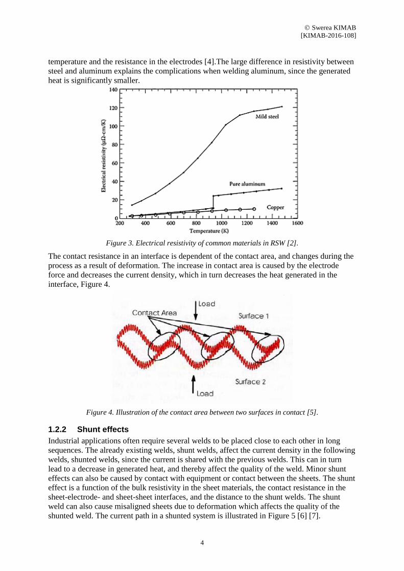
where R is resistance, ρ is resistivity, L is length and A is area. Values for the resistivity, as
afunction of temperature, in commonly used materials in RSW are illustrated in Figure 3.
Since the resistivity of steel and aluminum is larger than the resistivity of copper, the
generated heat in the sheets will be larger than the one in the electrodes. Likewise, the contact
resistance in the sheet-sheet interface will be larger than the one in the electrode-sheet
interface. Water cooling of the electrodes is used during the process to further reduce the
Swerea KIMAB
[KIMAB-2016-108]
4
temperature and the resistance in the electrodes [4].The large difference in resistivity between
steel and aluminum explains the complications when welding aluminum, since the generated
heat is significantly smaller.
Figure 3. Electrical resistivity of common materials in RSW [2].
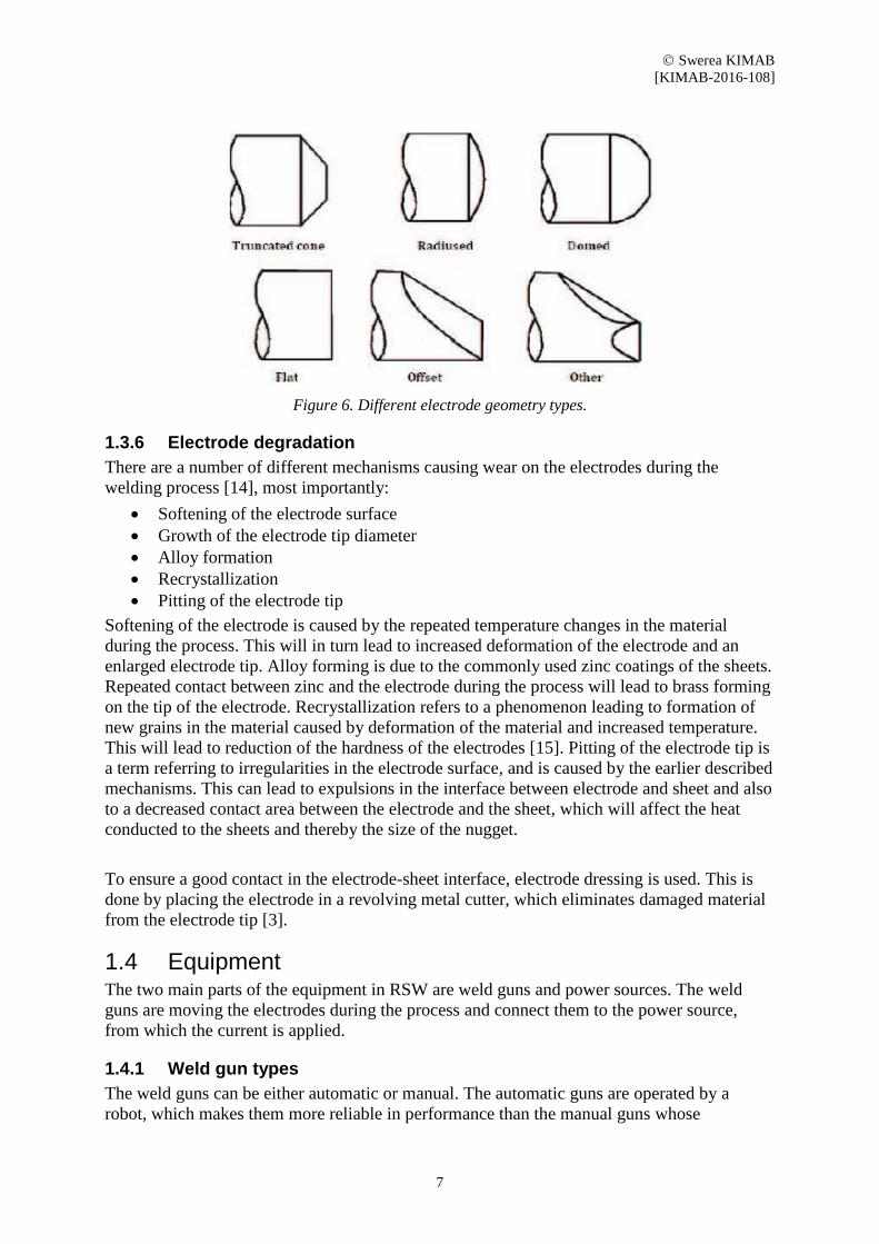
The contact resistance in an interface is dependent of the contact area, and changes during the
process as a result of deformation. The increase in contact area is caused by the electrode
force and decreases the current density, which in turn decreases the heat generated in the
interface, Figure 4.
Figure 4. Illustration of the contact area between two surfaces in contact [5].
1.2.2 Shunt effects
Industrial applications often require several welds to be placed close to each other in long
sequences. The already existing welds, shunt welds, affect the current density in the following
welds, shunted welds, since the current is shared with the previous welds. This can in turn
lead to a decrease in generated heat, and thereby affect the quality of the weld. Minor shunt
effects can also be caused by contact with equipment or contact between the sheets. The shunt
effect is a function of the bulk resistivity in the sheet materials, the contact resistance in the
sheet-electrode- and sheet-sheet interfaces, and the distance to the shunt welds. The shunt
weld can also cause misaligned sheets due to deformation which affects the quality of the
shunted weld. The current path in a shunted system is illustrated in Figure 5 [6] [7].

Swerea KIMAB
[KIMAB-2016-108]
5
Figure 5. Schematic picture of the current path in a shunted system [6].
1.2.3 Peltier effect
The Peltier effect is a physical phenomenon which affects the quality of the weld depending
of the direction of the current. When a current flows through the surface between two
different materials with different Fermi levels, the electrons will change orbits. This leads to
release or absorption of energy depending on the direction of the current. This phenomenon is
known as the Peltier effect. The heat generated by the Peltier effect can be written as,
t
p dttItQ0
)()( (1.4)
where Qp is the heat generated from the Peltier effect, I is the current, t is the time and ΠA and
ΠB is the Peltier coefficients for the materials in contact. The influence of the Peltier effect on
the weld result is smaller than the influence from the Joule effect, generally less than 10 % of
the generated heat. However, it can affect the result if the differences in Fermi levels of the
materials and the differences in thickness in the sheet stack-up are big. Studies have also
stated that the Peltier effect can decrease the electrode life [8] [9] [10].
1.3 Parameters in the RSW process The process of RSW depends on a number of input parameters. The most important
parameters are the weld current, the electrode force and the weld time. These parameters,
together with several other important factors are described in this chapter.
1.3.1 Weld current
The weld current is the dominant parameter in this welding process since the generated heat is
proportional to the square of the current. If the current is too high it may cause expulsion,
which in turn decreases the nugget size and causes splashes of molten material at other parts
of the construction, which then have to be removed and causes time-consuming repair work.
Using a current that is too high can also lead to large deformations and indentations on the

Swerea KIMAB
[KIMAB-2016-108]
6
sheets, as well as more wear on the electrodes. In contrast, a current that is too low will not
provide a satisfying nugget since the heat generation will be too low [2].
1.3.2 Electrode force
It is important to use a sufficient electrode force to produce contact between the sheets and
between the sheets and the electrodes during the process. If the electrode force is too large it
will lead to a decrease in contact resistance between the sheets, which in turn gives a decrease
in heat followed by a nugget that is either too small or non-existing. A too high electrode
force can also result in big indentations and bad visible quality. If the electrode force is too
small it will lead to an increase in contact resistance and may cause expulsion. The equipment
may be limiting if a high force is required. Common weld guns can apply forces up to 5 kN
[3] [11].
1.3.3 Weld time
The weld time is the time during which the current flows through the work pieces, and is
expressed as t in equation (1.1). A weld time that is too long may cause expulsion, while an
insufficient amount of time will result in lower heat generation and no nugget formation.
While using alternate current (AC), the weld time is measured in periods. However,
measuring the weld time in milliseconds has become more common due to the increased
popularity of direct current (DC).
In the automotive industry, the weld time is kept as short as possible to reduce the costs. As
implied by Joule’s law (1.1), a shorter weld time can be compensated by adjusting the weld
current [3].
1.3.4 Electrode material
The main functions of the electrodes are to squeeze the sheets together and to conduct
electricity and heat in the process. Therefore, the most important properties for the electrode
material are the compressive strength and the electrical and thermal conductivity. The most
common materials are copper and copper alloys. The electrode materials are described in the
standard ISO 5182:2008 [12].
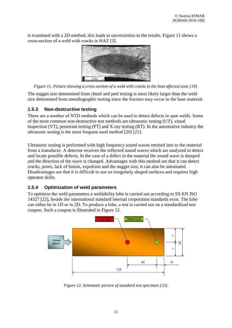
1.3.5 Electrode geometry
The geometry of the electrode tip determines the contact area between the electrode and the
sheets, which in turn affects both the contact pressure and the current density. A number of
common electrode geometries can be seen in Figure 6 .The geometry of the electrode should
be chosen according to the international standard ISO 5821:2009 [13].
Swerea KIMAB
[KIMAB-2016-108]
7
Figure 6. Different electrode geometry types.
1.3.6 Electrode degradation
There are a number of different mechanisms causing wear on the electrodes during the
welding process [14], most importantly:
Softening of the electrode surface
Growth of the electrode tip diameter
Alloy formation
Recrystallization
Pitting of the electrode tip
Softening of the electrode is caused by the repeated temperature changes in the material
during the process. This will in turn lead to increased deformation of the electrode and an
enlarged electrode tip. Alloy forming is due to the commonly used zinc coatings of the sheets.
Repeated contact between zinc and the electrode during the process will lead to brass forming
on the tip of the electrode. Recrystallization refers to a phenomenon leading to formation of
new grains in the material caused by deformation of the material and increased temperature.
This will lead to reduction of the hardness of the electrodes [15]. Pitting of the electrode tip is
a term referring to irregularities in the electrode surface, and is caused by the earlier described
mechanisms. This can lead to expulsions in the interface between electrode and sheet and also
to a decreased contact area between the electrode and the sheet, which will affect the heat
conducted to the sheets and thereby the size of the nugget.
To ensure a good contact in the electrode-sheet interface, electrode dressing is used. This is
done by placing the electrode in a revolving metal cutter, which eliminates damaged material
from the electrode tip [3].
1.4 Equipment The two main parts of the equipment in RSW are weld guns and power sources. The weld
guns are moving the electrodes during the process and connect them to the power source,
from which the current is applied.
1.4.1 Weld gun types
The weld guns can be either automatic or manual. The automatic guns are operated by a
robot, which makes them more reliable in performance than the manual guns whose

Swerea KIMAB
[KIMAB-2016-108]
8
performance is dependent on the operator. The kinetics of the guns is either electric or
pneumatic. The electric guns are more exact and generally more powerful; however they are
more expensive than the pneumatic guns. The most common gun arm types are linearly
moving C-guns and so called X-guns. Linear guns can operate within less space than the X-
guns and they do also provide a pure axial force, however the X-guns are less expensive [3].
Figure 7. X-gun connected to robot, used for the main part of the physical tests in this study [3].
1.4.2 Power sources
Earlier, alternate current (AC) were the dominant power source in RSW, however, mid
frequency direct current (MFDC) have become more frequently used recently. The MFDC
power sources have gained popularity since they both increase the nugget size and are more
energy efficient [3].
1.5 Weld quality and inspection According to American national standard (Standard welding terms and definitions,
ANSI/AWS A3.0:2001), no universal accepted standard for weld quality exist, however, an
acceptable weld is defined as “a weld that meets the applicable requirements”. The
determination of the weld quality is therefore mainly up to the manufacturer, and is done by
measuring a number of geometrical parameters. The most common parameters to measure are
listed below:
Nugget size
Penetration
Indentation
Cracks (internal and surface)
Porosity/voids

Swerea KIMAB
[KIMAB-2016-108]
9
Sheet separation
Surface appearance
Nugget size is the most indicative, and therefore also the most commonly used, of these
parameters. However, other parameters, such as penetration, are needed to fully investigate
the strength of the weld. Some of the above listed parameters are shown in Figure 8.
Figure 8. Cross-section of a spot weld, together with a number of quality evaluation parameters [2].
A relationship between the nugget diameter and the weld strength is showed in Figure 9, for
two 1.8 mm thick 780 MPa cold-rolled steel sheets. The figure shows the weld strength in
both tensile shear strength and cross tensile strength.
Figure 9. Shows the relationship between nugget diameter and weld strength in two 1.8 mm thick 780
MPa cold-rolled steel sheets in both tensile shear strength and cross tensile strength [16].
Different manufacturers and organizations have their own requirements and standards
regarding nugget sizes and indentations. However, most corporation standards states that a
nugget size of 3,5√h-5√h is demanded, where h is the minimum thickness in the sheet stack-
up [2] [17].
1.5.1 Testing procedures
A number of testing procedures can be used in order to determine the relevant parameters.
There are two main categories of testing procedures for spot welds; destructive testing and
non-destructive testing. The most common way to inspect the quality of the weld is to
measure the nugget size and determine the failure mode.

Swerea KIMAB
[KIMAB-2016-108]
10
1.5.2 Destructive testing
Chisel test, peel test, and metallographic test are the main destructive testing procedures.
These are described below.
1.5.2.1 Chisel test
The chisel test can be carried out both as a destructive- and a non-destructive test method.
When carried out as a destructive testing method a chisel is driven in between the sheets
either until fracture or major deformation occurs. This is done to reveal the weld plug and
enable measuring of the plug size. If the weld contains more than two sheets, the test shall be
carried out for every interface.
The non-destructive chisel test is also carried out with a chisel driven in between the sheets.
However, in this case the chisel is just driven in until the material adjacent to the weld bends
or yields. This is done to assure fracture has not occurred close to, or in the weld. If it is
determined that fracture has not occurred, the sheets shall be restored to the original shape
again. As in the destructive testing procedure this test shall be carried out in all interfaces in
the weld [18].
1.5.2.2 Peel test
The peel test can only be carried out as a destructive testing method. This test is performed by
slowly pealing the sheets apart until all the welds that will be investigated are fully fractured.
The most common way to perform this test is by locking one of the sheets to a vice and then
peel the sheets apart with either a roller tool or a plier.
In both the chisel test and the peel test the plug size is measured with a caliper. Both the
maximum and the minimum diameter are measured and the mean diameter is used to account
for irregularities and non-circular welds [18].
A schematic picture of the chisel test and the peel test, both with roller tool and plier, is
shown in Figure 10.
Figure 10. Schematic picture of the chisel test (a) and the peel test, both with roller tool (b) and plier
(c) [18].
1.5.2.3 Metallographic testing
In order to examine the appearance of voids and cracks in the weld and the heat affected zone,
HAZ, a metallographic test can be performed. This is carried out by cutting through the center
of the weld and then polishing the surface. The weakness in this method is that a 3D-structure
Swerea KIMAB
[KIMAB-2016-108]
11
is examined with a 2D-method, this leads to uncertainties in the results. Figure 11 shows a
cross-section of a weld with cracks in HAZ [3].
Figure 11. Picture showing a cross-section of a weld with cracks in the heat affected zone [19].
The nugget size determined from chisel and peel testing is most likely larger than the weld
size determined from metallographic testing since the fracture may occur in the base material.
1.5.3 Non-destructive testing
There are a number of NTD methods which can be used to detect defects in spot welds. Some
of the most common non-destructive test methods are ultrasonic testing (UT), visual
inspection (VT), penetrant testing (PT) and X-ray testing (RT). In the automotive industry the
ultrasonic testing is the most frequent used method [20] [21].
Ultrasonic testing is performed with high frequency sound waves emitted into to the material
from a transducer. A detector receives the reflected sound waves which are analyzed to detect
and locate possible defects. In the case of a defect in the material the sound wave is damped
and the direction of the wave is changed. Advantages with this method are that it can detect
cracks, pores, lack of fusion, expulsion and the nugget size, it can also be automated.
Disadvantages are that it is difficult to use on irregularly shaped surfaces and requires high
operator skills.
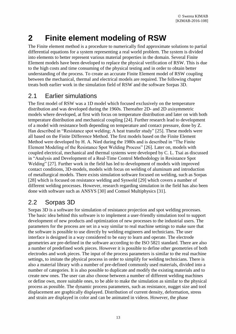
1.5.4 Optimization of weld parameters
To optimize the weld parameters a weldability lobe is carried out according to SS-EN ISO
14327 [22], beside the international standard internal corporation standards exist. The lobe
can either be in 1D or in 2D. To produce a lobe, a test is carried out on a standardized test
coupon. Such a coupon is illustrated in Figure 12.
Figure 12. Schematic picture of standard test specimen [23].

Swerea KIMAB
[KIMAB-2016-108]
12
As shown in Figure 12 two spots are welded on the coupon, however, it is only the test spot
which is examined. To produce a 1D-lobe the test is performed by keeping the electrode force
and the weld time constant while increasing the current stepwise with 0,3 kA. For each step
three spots are welded. If one of the spots splashes or spatter two more shall be done. The test
is stopped if two of the spots splashes or spatter. The result is presented as in Figure 13, the
lobe shall show the minimum required nugget diameter, decided as a function of the
minimum sheet thickness as mentioned above. The least acceptable current range, process
window, is 1,2 kA.
Figure 13.Illustration of a 1D-lobe.
A 2D-lobe is carried out in the same way; however, in this case two of the three parameters
are varied. The result is presented as in Figure 14 [3] [23].
Figure 14.Illustration of a 2D-lobe.
Swerea KIMAB
[KIMAB-2016-108]
13
2 Finite element modeling of RSW The Finite element method is a procedure to numerically find approximate solutions to partial
differential equations for a system representing a real world problem. The system is divided
into elements to better represent various material properties in the domain. Several Finite
Element models have been developed to replace the physical verification of RSW. This is due
to the high costs and time consuming of the physical testing and in order to obtain better
understanding of the process. To create an accurate Finite Element model of RSW coupling
between the mechanical, thermal and electrical models are required. The following chapter
treats both earlier work in the simulation field of RSW and the software Sorpas 3D.
2.1 Earlier simulations The first model of RSW was a 1D model which focused exclusively on the temperature
distribution and was developed during the 1960s. Thereafter 2D- and 2D axisymmetric
models where developed, at first with focus on temperature distribution and later on with both
temperature distribution and mechanical coupling [24]. Further research lead to development
of a model with resistance both depending on temperature and contact pressure, done by Z.
Han described in “Resistance spot welding; A heat transfer study” [25]. These models were
all based on the Finite Difference Method. The first models based on the Finite Element
Method were developed by H. A. Nied during the 1980s and is described in “The Finite
Element Modeling of the Resistance Spot Welding Process” [26]. Later on, models with
coupled electrical, mechanical and thermal systems were developed by C. L. Tsai as discussed
in “Analysis and Development of a Real-Time Control Methodology in Resistance Spot
Welding” [27]. Further work in the field has led to development of models with improved
contact conditions, 3D-models, models with focus on welding of aluminum and introduction
of metallurgical models. There exists simulation software focused on welding, such as Sorpas
[28] which is focused on resistance welding and Sysweld [29] which covers a number of
different welding processes. However, research regarding simulation in the field has also been
done with software such as ANSYS [30] and Comsol Multiphysics [31].
2.2 Sorpas 3D Sorpas 3D is a software for simulation of resistance projection and spot welding processes.
The basic idea behind this software is to implement a user-friendly simulation tool to support
development of new products and optimization of new processes to the industrial users. The
parameters for the process are set in a way similar to real machine settings to make sure that
the software is possible to use directly by welding engineers and technicians. The user
interface is designed in a way considered to be easy to learn and operate. The electrode
geometries are pre-defined in the software according to the ISO 5821 standard. There are also
a number of predefined work pieces. However it is possible to define other geometries of both
electrodes and work pieces. The input of the process parameters is similar to the real machine
settings, to imitate the physical process in order to simplify for welding technicians. There is
also a material library with a number of pre-defined commonly used materials, divided into a
number of categories. It is also possible to duplicate and modify the existing materials and to
create new ones. The user can also choose between a number of different welding machines
or define own, more suitable ones, to be able to make the simulation as similar to the physical
process as possible. The dynamic process parameters, such as resistance, nugget size and tool
displacement are graphically displayed. Distribution of current density, deformation, stress
and strain are displayed in color and can be animated in videos. However, the phase

Swerea KIMAB
[KIMAB-2016-108]
14
transformations are not considered in the software, which implies that the stresses and strains
during cooling might be inaccurate, due to martensite transformations [32].
2.2.1 Model setup
In the 3D version of the software the model is built up like shown in Figure 15. Pre-defined
objects for the electrodes and work pieces are chosen, the thickness of coatings and interfaces
are defined and materials for electrodes, work pieces and coatings are selected from the
material library.
Figure 15. 3D simulation model with electrodes, work pieces, coatings and interfaces.
Likewise, it is possible to insert existing connections to create a model with pre-existing weld
nuggets or shunt connections as shown in Figure 16. The added existing connections are
cylinders defined by diameter, height and initial temperature. A simulation with pre-welded
nuggets or shunt connections calculates the current through each weld and the result is
presented graphically together with the other dynamic process parameters.
Swerea KIMAB
[KIMAB-2016-108]
15
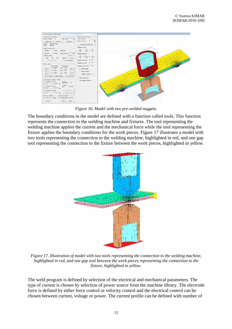
Figure 16. Model with two pre-welded nuggets.
The boundary conditions in the model are defined with a function called tools. This function
represents the connection to the welding machine and fixtures. The tool representing the
welding machine applies the current and the mechanical force while the tool representing the
fixture applies the boundary conditions for the work pieces. Figure 17 illustrates a model with
two tools representing the connection to the welding machine, highlighted in red, and one gap
tool representing the connection to the fixture between the work pieces, highlighted in yellow.
Figure 17. Illustration of model with two tools representing the connection to the welding machine,
highlighted in red, and one gap tool between the work pieces representing the connection to the
fixture, highlighted in yellow.
The weld program is defined by selection of the electrical and mechanical parameters. The
type of current is chosen by selection of power source from the machine library. The electrode
force is defined by either force control or velocity control and the electrical control can be
chosen between current, voltage or power. The current profile can be defined with number of

Swerea KIMAB
[KIMAB-2016-108]
16
pulses and up- and down slope of the current at each pulse. The welding program is displayed
graphically with curves as shown in Figure 18.
Figure 18. Illustration of defined weld program with electrode force in the upper window and current
profile in the lower window.
2.2.2 Capabilities and limitations
In contrast to Sorpas 2D, Sorpas 3D has the capability to simulate shunt effects and
misalignments. The shunt effects can be simulated both with a series of welds and with pre-
welded nuggets. Results from simulations of shunt effects are presented in chapter 3.7 and
results from simulations with misalignments are presented in chapter 3.8.
The 3D edition also provides the possibility to perform weld strength testing, such as tensile-
shear, cross-tension and peel testing. Likewise it is possible to simulate cases with complex
geometries.
However, there are still a number of functions yet to come in the 3D edition. It is not yet
possible to detect expulsion, which in turn leads to the fact that generation of weldability
lobes is not possible. The 2D edition provides the possibility to investigate the Peltier effect
on the weld result; this is not yet possible in the 3D edition. However, the accuracy of the
expulsion criterion and the simulation of the Peltier effect in Sorpas 2D is not investigated in
this study.
2.3 Numerical model To fully represent the RSW process, coupling between the electrical, mechanical and thermal
model is required. Since Sorpas 3D is a commercial software not all of the numerical code is
revealed. However, this chapter describes the official information about the models,
separately as well as the coupling between them.
2.3.1 Mechanical module
The weak variation form of the irreducible flow formulation,

Swerea KIMAB
[KIMAB-2016-108]
17
V St
ciijjii
V
dSutdVKdV 0 (2.1)
is the base for the mechanical module. The first term describes the energy rate caused by
plastic deformation in the domain volume, V, the second term covers the constraint of
incompressibility, the third term describes the traction over the surface St and the fourth term
describes the contact, further explained in chapter 2.3.4. is the effective stress according to
von Mises, is the effective plastic strain rate, identifies the variations in velocities, ii is
the volumetric strain rate, K is a penalty factor, described by a large positive number and it
are prescribed surface tractions. The penalty factor, K, is related to the mean stress as,
mkkK 2 (2.2)
The accumulation of damage in mechanical strength simulations are modeled with
constitutive equations of metallic materials with porosity. The yield criterion is,
12
2 BIAJR (2.3)
where J2 is the second invariant of the deviatoric stress tensor, I1 is the first invariant of the
stress tensor, 2
R is the effective stress response to a given relative density R, and given by,
CR (2.4)
where is the effective stress response to a fully dense material. The constants A, B and C
depend on the relative density.
2.3.2 Thermal module
The thermal module follows,
V V S
SVmmi
V
i dSqTdVqTdVTcdVTkT 0,, (2.5)
and is based on classical Galerkin treatment of heat transfer. The first term is the heat
conduction in the volume V, the second term represents the stored energy linked to the
temperature rate, the third term describes the heat generation rate in the volume V and the
fourth term describes the heat generation rate, or the heat loss rate, at the surface, S. The fifth
term ensures the same temperature on both sides of contact interfaces and is described in
chapter 2.3.4. In (2.5), k is the thermal conductivity, ρm is the mass density, cm is the heat
capacity and δ identifies the temperature variations.
Both the plastic work and the Joule heating contributes to the heat generation as shown in,

Swerea KIMAB
[KIMAB-2016-108]
18
2Jq
q
Joule
plastic
(2.6)
where β is a factor describing the transformation of mechanical energy into heat, usually it is
assumed to be in the range of 0,85 to 0,95, ρ is the electrical resistivity and J is the current
density, given in (2.9).
The heat generation rate at the surfaces depends on friction, convection and radiation as,
)(
)(
44
fsSBemisradiation
fsconvection
rffriction
TTq
TThq
vq
(2.7)
where f is the friction shear stress, vr is the relative sliding speed of the two surfaces, h is the
heat transfer coefficient, Ts is the temperature of the surface, Tf is the temperature of the
surroundings, emis is the emissivity coefficient and SB is the Stefan-Boltzmann constant.
2.3.3 Electrical module
The major variable in the electrical module is the electrical potential, Φ. The governing
equation for the electrical module can be written as,
S
n
V
ii dSdV 0,,, (2.8)
The third term in (2.8) represents the contact between objects and is described in chapter
2.3.4. However, (2.8) can be simplified by setting the second term equal to zero since the
gradient of the potential along a free surface is zero, which in turn results in the electrical
potential being determined only by the geometry. At the boundaries with power supply the
electrical potential is set to Φ0 and at free boundaries the electrical potential is equal to zero.
The current density, J, is a function of the electrical potential gradient and the electrical
resistivity as,
i
iJ,
(2.9)
2.3.4 Contact modeling
The contact conditions can be separated into mechanical, electrical and thermal. The
mechanical contact can in turn be divided into normal and tangential constraint. The fourth
term in (2.1) is written as,
C CN
c
N
c
c
t
c
t
c
n
c
nC ggPggP1 1
(2.10)
Where c
ng is the normal gap velocities, c
tg is the tangential gap velocities and P is a penalty
factor. The first term is active to ensure no penetration between surfaces and also when

Swerea KIMAB
[KIMAB-2016-108]
19
contact pairs are identified as welded and inactive when two surfaces separates. The second
term is active when full sticking conditions between surfaces are simulated and also in already
welded contact pairs, the second term is inactive when frictionless or frictional sliding is
chosen.
The frictional shear stress is modeled by combining the Amonton-Coulomb law,
nf (2.11)
and the law of constant friction,
mkf (2.12)
where μ is the friction coefficient, n is the normal pressure, m is the friction factor and k is
the shear flow stress.
To ensure the same electrical potential and temperature on both sides of contact interfaces the
penalty terms in
C
C
N
c
c
d
c
dT
N
c
c
d
c
d
TTP
P
1
1
(2.13)
are used to describe the fifth term in (2.5) and the third term in (2.8).
The contact resistivity is described as,
antconta
n
soft
c min21
2
3
(2.14)
where the fraction of soft and n represents the contact area, soft is the flow stress of the
softer of the two materials in contact and n is the normal pressure. 1 and 2 are the bulk
resistivities of the materials in contact and antcontamin covers the contribution to the resistance
from surface contaminants.
2.3.5 Electro-thermo-mechanical couplings
The mechanical, thermal and electrical modules are coupled together as shown in Figure 19.
First the mechanical module is run at each time step to calculate the velocities, geometrical
changes, contact areas and stress responses, since it affects the electrical and thermal modules
in terms of deformation heat, friction generated heat and electrical and thermal contact
properties affected by the contact stresses. The electrical module affects the thermal module
since the output of the electrical module is the current density which is the dominant factor in
the Joule heating. After individual and mutual convergence is reached the output from the
thermal module updates the temperature dependent material properties

Swerea KIMAB
[KIMAB-2016-108]
20
Figure 19. Schematic picture of the electro-thermo-mechanical coupling [24].
The weaker coupling with the mechanical module, compared to the coupling between the
electrical and the thermal module, is compensated by small time steps in the simulation. The
small time steps ensure minimal errors in the mechanical module and the time saving because
of the weak coupling is considered as large [24] [33].
2.4 Material data To achieve sufficiently accurate results from the simulations a number of material data are
needed. In order to reach a high accuracy in the simulation results, the material data needs to
be functions of temperature and also take the phase transformation into account. In this
chapter the Sorpas default material data are compared to data from the literature, which also is
used in the simulations. The materials used in the comparison between simulations and
physical testing are presented in Table 1. These materials are classified as Ultra High Strength
Steels, UHSS, and High Strength Steels, HSS. They are commonly used in the automotive
industry in order to minimize weight in the construction with maintained strength.
Table 1. Material, coatings and thickness for the sheets used in comparison between simulations and
physical testing.
Sheet material Coating Thickness [mm] σy [MPa]
Usibor 1500P AS75/75 1.2-2 1200
Mild Steel GI50/50 or uncoated 0.6-1 170
DP600 GI50/50 or uncoated 1.2-2 410
DP800 GI50/50 1.2 570
Table 2. Chemical composition of materials used in this work, values in wt% [29].
Material C Si Mn P S N Cr Ni Cu Mo Al Nb V Ti B
Usibor 1500P
0.226 0.26 1.17 0.009 0.005 - 0.22 0.038 0.014 - 0.048 0.013 0.036 0.003
Mild Steel 0.13 0.23 1.51 0.009 0.003 0.005 0.03 0.05 0.01 - 0.05 0.02 - - -
DP600 0.1 0.21 1.62 0.008 0.002 0.006 0.47 0.04 0.01 - 0.05 - - -
DP800 0.15 0.2 1.72 0.012 0.003 0.005 0.42 0.04 0.01 - 0.04 0.02 - - -

Swerea KIMAB
[KIMAB-2016-108]
21
The material parameters which have been modified in the material database to provide a
better agreement between the simulations and the physical testing are; thermal conductivity,
specific heat capacity, resistivity and flow stress. The results from the investigation of these
material properties impact on the result is presented in chapter 3.3.
2.4.1 Thermal conductivity
The propagation of the heat generated by (1.1) is related to the thermal conductivity of the
materials. The accuracy of the thermal conductivity is of high importance for the simulation
results. The literature values for the thermal conductivity are calculated with a software called
IDS, which uses the chemical composition of the material to estimate the thermal conductivity
of the material [29]. A comparison of the thermal conductivity between the default values in
Sorpas 3D and the values from the IDS calculations of the four different materials are shown
in Figure 20. There exist more accurate methods to examine the thermal conductivity of
materials. One method is the Laser Flash method, which is performed by heating the front
side of a sample with a short laser pulse and measuring the temperature rise on the rear side
[34].
Figure 20. Comparison of thermal conductivity between Sorpas default values and IDS calculated
values for: (a) DP600, (b) Mild steel, (c) Usibor 1500P and (d) DP800.
2.4.2 Specific heat capacity
The temperature in the system is of high importance to generate correct simulation results, as
mentioned in chapter 2.3.5. The specific heat capacity is the amount of heat energy, required
to raise the temperature of a certain amount of mass with one Kelvin. To be able to determine
the temperature in each time step the accuracy of the specific heat capacity is important. A
comparison between the Sorpas 3D values and values calculated with the software
ThermoCalc is presented in Figure 21. ThermoCalc is a software using the chemical
composition of the material to calculate the specific heat capacity [29].

Swerea KIMAB
[KIMAB-2016-108]
22
Figure 21. Comparison of specific heat capacity between Sorpas default values and ThermoCalc
calculated values for: (a) DP600, (b) Mild Steel, (c) Usibor1500P and (d) DP800.
2.4.3 Resistivity
The resistivity of a material is highly dependent on the temperature. The values for DP600 are
known from literature and differences between steel materials are considered to be small,
therefore the literature values for DP600 are used for all materials in this study. A comparison
between the values from Sorpas 3D and the values from the literature is shown in Figure 22
[29] [5].
Figure 22. Comparison of resistivity between Sorpas default values and literature values [29].
2.4.4 Flow stress
The flow stress has a major impact on the simulation results since it affects the contact areas
in the sheet-sheet interfaces and the sheet-electrode interfaces. The contact areas in the sheet-
sheet interfaces affect the contact resistance as shown in (2.14) and the contact areas in the
sheet-electrode interfaces affect the cooling from the electrodes. A comparison of the flow

Swerea KIMAB
[KIMAB-2016-108]
23
stress curves for the four materials listed in Table 1 for the default values from Sorpas and the
literature is shown in Figure 23, Figure 24, Figure 25 and Figure 26 [29]. As illustrated in
these figures, the main difference between these values is the quicker drop in flow stress with
respect to temperature for the literature values compared to the Sorpas default values. The
decreased flow stress increases the cooling from the electrodes during the welding process.
Figure 23. Flow stress curves from Sorpas and literature for DP600 from 20 to 1400 °C.
Figure 24. Flow stress curves from Sorpas and literature for Mild steel from 20 to 1400°C.
Figure 25. Flow stress curves from Sorpas and literature for Usibor from 20 to 1400 °C.
Figure 26. Flow stress curves from Sorpas and literature for DP800 from 20 to 1400 °C.
Swerea KIMAB
[KIMAB-2016-108]
24
3 Results In order to evaluate the usefulness of the software and to investigate its limitations a number
of tests have been performed. In the following chapter these tests are described and the results
are presented.
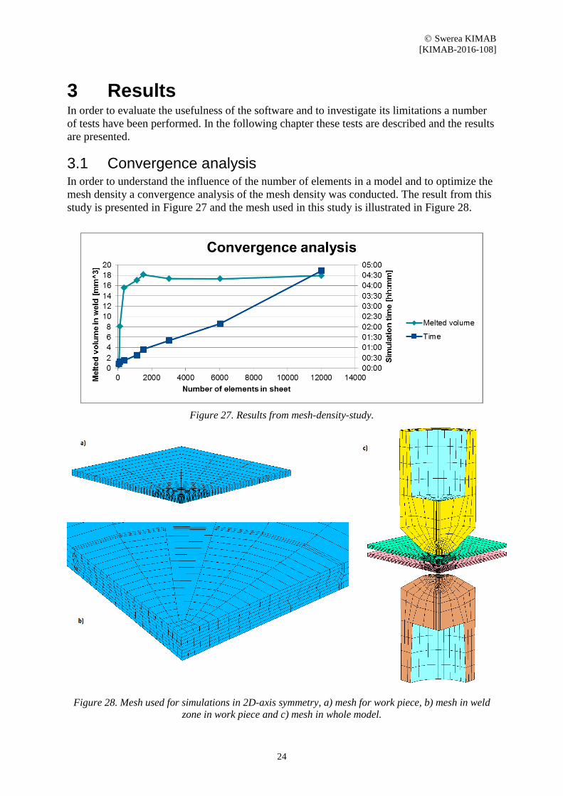
3.1 Convergence analysis In order to understand the influence of the number of elements in a model and to optimize the
mesh density a convergence analysis of the mesh density was conducted. The result from this
study is presented in Figure 27 and the mesh used in this study is illustrated in Figure 28.
Figure 27. Results from mesh-density-study.
Figure 28. Mesh used for simulations in 2D-axis symmetry, a) mesh for work piece, b) mesh in weld
zone in work piece and c) mesh in whole model.

Swerea KIMAB
[KIMAB-2016-108]
25
3.2 Simulations To examine the accuracy of the default settings in the software and in order to trace possible
changes in the settings, a number of simulations were run. The following chapter describes
these simulations and the modifications done in order to make the simulations more realistic.
3.2.1 Default settings
The software contains a number of pre-created models. The least complex of these models
were called 2-sheet-spot-welding and are described in Table 3, Table 4 and Table 5. The
process for this simulation is shown in Figure 29.
Table 3. Materials and geometries in 2-sheet-spot-welding.
Material Coating Thickness [mm]
Sheet 1 Mild Steel Uncoated (UC) 1
Sheet 2 Mild Steel Uncoated (UC) 1
Table 4. Material and geometry for electrodes used in 2-sheet-spot-welding.
Material Geometry
A2/2-Cap F-Cap 16/6
Table 5. Process parameters used in 2-sheet-spot-welding.
Force [kN] Squeeze Time [ms] Current [kA] Weld Time [ms] Hold Time [ms]
3 60 8 160 40
Figure 29. Simulations of 2-sheet-spot-welding when, (a) the current is turned on, t=65 ms, (b) the
first melt is formed, t=105 ms and (c), the final nugget, t=220 ms.

Swerea KIMAB
[KIMAB-2016-108]
26
A more complex pre-created model, 3-sheet-spot-welding, were then simulated. The
materials, geometries and process parameters for this case is described in Table 6, Table 7 and
Table 8.
Table 6. Materials and geometries in 3-sheet-spot-welding.
Material Coating Thickness [mm]
Sheet 1 Mild Steel GI50/50 0.8
Sheet 2 HSLA 340 GI50/50 1.2
Sheet 3 DP600 GI50/50 1.5
Table 7. Material and geometry for electrodes used in 3-sheet-spot-welding.
Material Geometry
A2/2-Cap F-Cap 16/6
Table 8. Process parameters used in 3-sheet-spot-welding.
Force
[kN]
Squeeze time
[ms]
1-current
[kA]
1-time
[ms]
1-puase
[ms]
2-current
[kA]
2-time
[ms]
2-pause
[ms]
3-current
[kA]
3-time
[ms]
3.73 120 10.435 160 40 10.435 160 40 10.435 160
Figure 30 shows the first formed melt in 3-sheet-spot-welding. As seen in the figure, the melt
is formed within one of the sheets instead of in one of the interfaces between the sheets. A
number of similar tests were made to investigate why this phenomenon occur. The outcome
of these tests resulted in a number of modifications in the material data. The tests and the
outcome of them are more discussed in chapter 4.
Figure 30. First formed melt in 3-sheet-spot-welding, t=170 ms.

Swerea KIMAB
[KIMAB-2016-108]
27
3.2.2 Simulations with modified material properties
The modifications in coating properties resulted in a process where the first melt occurred in
the sheet-to-sheet interface, however, with a non-lens shaped nugget, as illustrated in Figure
31. Further modifications with especially the yield strength for the sheets materials resulted in
a process shown in Figure 32, with the first melt formed in the sheet-to-sheet interface and a
lens shaped nugget. However, the resistivity, thermal conductivity and specific heat capacity
were also modified. Materials, geometries and process parameters for this case is described in
Table 9, Table 10 and Table 11.
Table 9. Materials and geometries in HSS-2T.
Material Coating Thickness [mm]
Sheet 1 Mild Steel GI50/50 0.7
Sheet 2 Usibor 1500P AS75/75 1.8
Table 10. Material and geometry for electrodes used in HSS-2T.
Material Geometry
A2/2-Cap B-Cap 20/8
Table 11. Process parameters used in HSS-2T.
Force [kN] 1-Current [kA] 1-time [ms] 1-pause [ms] 2-Current [kA] 2-time [ms]
2.3 7 100 40 7.5 290
Figure 31. First formed melt and development of non-lens shaped nugget in HSS-2T, for time steps 80
and 470 ms respectively.

Swerea KIMAB
[KIMAB-2016-108]
28
Figure 32. First formed melt and development of lens shaped nugget in HSS-2T, time steps 80 and 470
ms respectively.
The modified material properties are those presented as literature and calculated values in
chapter 2.4. These data are used in all the simulations described below.
3.3 Impact of material data A number of tests have been performed to investigate which material parameters are the most
important to examine when new materials are to be used in the simulations. The investigated
material parameters are the one discussed in chapter 2.4. The tests have consisted of two 1
mm thick sheets in three different materials. Each sheet combination has been simulated
seventeen times, first with the original material parameters and then every parameter has been
increased or decreased with ten and twenty percent with all other input parameters kept
constant. The results from these simulations are presented in Figure 33, where the changes in
material data are compared to the percentage differences in melted volume in the weld. The
upper diagram shows the difference in melted volume when the material properties are
changed with ten percent and the lower diagram shows the differences in melted volume
when the material properties are changed with twenty percent.

Swerea KIMAB
[KIMAB-2016-108]
29
Figure 33. Percentage difference in melted volume in weld due to variation in material properties.
3.4 1D-lobes In order to compare the results from the simulations to the results from the physical tests a
number of 1D-lobes with both simulated and physically tested results were carried out. The
cases vary in geometry, material and number of sheets to investigate the validity of the
simulations in both simpler and more complex cases. The different cases and the results are
presented below. The simulation time for these four 1D-lobes are presented in Table 12. All
the simulations are performed on a computer with Windows 7, 16 GB RAM, 3,5 GHz 16P.
Table 12. Simulation time for the four 1D-lobes in chapter 3.4.
Case Uncoated UHSS-3T UHSS-3T UHSS-4T
Time [hh:mm:ss] 15:34:19 22:56:55 15:05:33 71:04:41
Process time for 1
weld [ms]
400 480 670 800
Number of welds
in 1D-lobe
14 14 6 12
Swerea KIMAB
[KIMAB-2016-108]
30
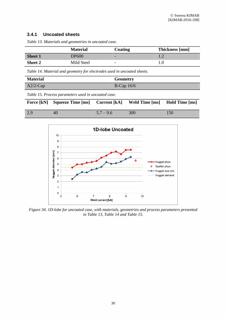
3.4.1 Uncoated sheets
Table 13. Materials and geometries in uncoated case.
Material Coating Thickness [mm]
Sheet 1 DP600 - 1.2
Sheet 2 Mild Steel - 1.0
Table 14. Material and geometry for electrodes used in uncoated sheets.
Material Geometry
A2/2-Cap B-Cap 16/6
Table 15. Process parameters used in uncoated case.
Force [kN] Squeeze Time [ms] Current [kA] Weld Time [ms] Hold Time [ms]
2.9 40 5.7 – 9.6 300 150
Figure 34. 1D-lobe for uncoated case, with materials, geometries and process parameters presented
in Table 13, Table 14 and Table 15.

Swerea KIMAB
[KIMAB-2016-108]
31
Figure 35. Comparison of simulated and
physically conducted nugget size. Materials,
geometries and process parameters as
presented in Table 13, Table 14 and Table 15.
Figure 36. Final nugget in uncoated case,
second current set to 9,3 kA.
3.4.2 UHSS-3T
Table 16. Materials and geometries in UHSS-3T.
Material Coating Thickness [mm]
Sheet 1 Usibor 1500P AS75/75 1.6
Sheet 2 DP600 - 1.15
Sheet 3 Usibor 1500P AS75/75 1.4
Table 17. Material and geometry for electrodes used in UHSS-3T.
Material Geometry
A2/2-Cap B-Cap 16/6
Table 18. Process parameters used in UHSS-3T.
Force [kN] 1-Current [kA] 1-time [ms] 1-pause [ms] 2-Current [kA] 2-time [ms]
4.0 8.0 100 80 5.7 – 9.6 300

Swerea KIMAB
[KIMAB-2016-108]
32
Figure 37. 1D-lobe for UHSS-3T, with materials, geometries and process parameters as presented in
Table 16, Table 17 and Table 18.
Figure 38. Comparison of simulated and
physically conducted nugget size. Materials,
geometries and process parameters presented
in Table 16, Table 17 and Table 18.
Figure 39. Final nugget in UHSS-3T, second
current set to 9 kA.
3.4.3 UHSS-2T
Table 19. Materials and geometries in UHSS-2T.
Material Coating Thickness [mm]
Sheet 1 DP600 GI50/50 2
Sheet 2 Usibor 1500P AS75/75 1.4
Table 20. Material and geometry for electrodes used in UHSS-2T.
Material Geometry
A2/2-Cap B-Cap 20/8

Swerea KIMAB
[KIMAB-2016-108]
33
Table 21. Process parameters used in UHSS-2T.
Force [kN] 1-Current [kA] 1-time [ms] 1-pause [ms] 2-Current [kA] 2-time [ms]
4.6 10.5 100 40 7.8 – 9.3 430
Figure 40. 1D-lobe for UHSS-2T, with materials, geometries and process parameters presented in
Table 19, Table 20 and Table 21.
Figure 41. Comparison of simulated and
physically conducted nugget size. Materials,
geometries and process parameters as
presented in Table 19, Table 20 and Table 21.
Figure 42. Final nugget in UHSS-2T, second
current set to 9 kA.

Swerea KIMAB
[KIMAB-2016-108]
34
3.4.4 UHSS-4T
Table 22. Materials and geometries in UHSS-4T.
Material Coating Thickness [mm]
Sheet 1 DP600 GI50/50 1.5
Sheet 2 Mild Steel GI50/50 0.7
Sheet 3 Mild Steel GI50/50 0.6
Sheet 4 Usibor 1500P AS75/75 1.7
Table 23. Material and geometry for electrodes used in UHSS-4T.
Material Geometry
A2/2-Cap B-Cap 20/8
Table 24. Process parameters used in UHSS-4T.
Force [kN] 1-Current [kA] 1-time [ms] 1-pause [ms] 2-Current [kA] 2-time [ms]
4.0 11.0 100 40 7.2 – 10.8 560
Figure 43. 1D-lobe for UHSS-4T, with materials, geometries and process parameters as presented in
Table 22, Table 23 and Table 24.
Swerea KIMAB
[KIMAB-2016-108]
35
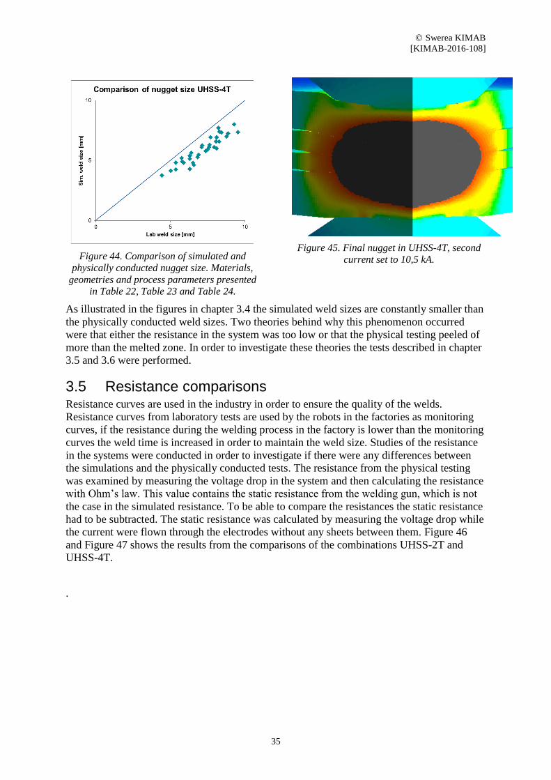
Figure 44. Comparison of simulated and
physically conducted nugget size. Materials,
geometries and process parameters presented
in Table 22, Table 23 and Table 24.
Figure 45. Final nugget in UHSS-4T, second
current set to 10,5 kA.
As illustrated in the figures in chapter 3.4 the simulated weld sizes are constantly smaller than
the physically conducted weld sizes. Two theories behind why this phenomenon occurred
were that either the resistance in the system was too low or that the physical testing peeled of
more than the melted zone. In order to investigate these theories the tests described in chapter
3.5 and 3.6 were performed.
3.5 Resistance comparisons Resistance curves are used in the industry in order to ensure the quality of the welds.
Resistance curves from laboratory tests are used by the robots in the factories as monitoring
curves, if the resistance during the welding process in the factory is lower than the monitoring
curves the weld time is increased in order to maintain the weld size. Studies of the resistance
in the systems were conducted in order to investigate if there were any differences between
the simulations and the physically conducted tests. The resistance from the physical testing
was examined by measuring the voltage drop in the system and then calculating the resistance
with Ohm’s law. This value contains the static resistance from the welding gun, which is not
the case in the simulated resistance. To be able to compare the resistances the static resistance
had to be subtracted. The static resistance was calculated by measuring the voltage drop while
the current were flown through the electrodes without any sheets between them. Figure 46
and Figure 47 shows the results from the comparisons of the combinations UHSS-2T and
UHSS-4T.
.

Swerea KIMAB
[KIMAB-2016-108]
36
Figure 46. Comparison of resistance between simulation and physical test for UHSS-2T.
Figure 47. Comparison of resistance between simulation and physical test for UHSS-4T.
3.6 Cross-section comparison Comparisons of the simulated and physically conducted cross-sections of the welds were done
in order to further investigate possible reasons to the differences in the results. The materials,
geometries and process parameters for these tests are presented in Table 25,Table 26,Table 27
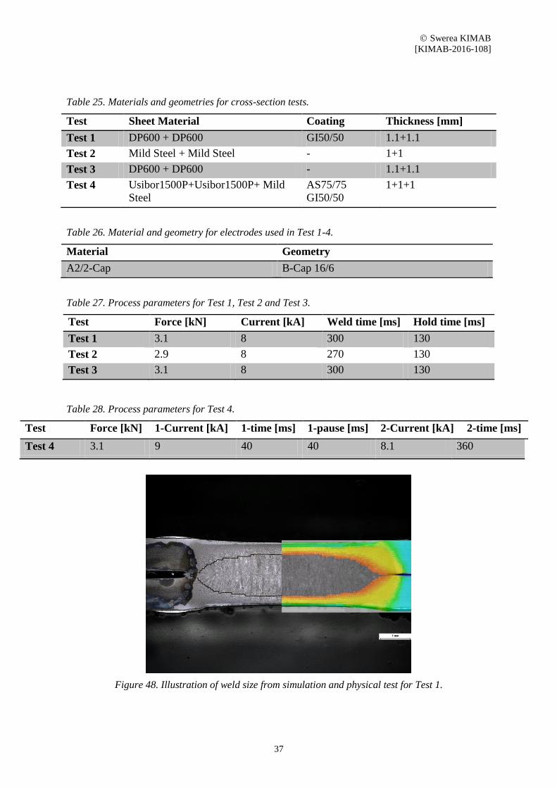
and Table 28. The results are presented in Figure 52. Figure 48, Figure 49, Figure 50 and
Figure 51 illustrates the cross-sections of the physically conducted welds with simulations
pasted on top together with a black line also representing the simulations.
Swerea KIMAB
[KIMAB-2016-108]
37
Table 25. Materials and geometries for cross-section tests.
Test Sheet Material Coating Thickness [mm]
Test 1 DP600 + DP600 GI50/50 1.1+1.1
Test 2 Mild Steel + Mild Steel - 1+1
Test 3 DP600 + DP600 - 1.1+1.1
Test 4 Usibor1500P+Usibor1500P+ Mild
Steel
AS75/75
GI50/50
1+1+1
Table 26. Material and geometry for electrodes used in Test 1-4.
Material Geometry
A2/2-Cap B-Cap 16/6
Table 27. Process parameters for Test 1, Test 2 and Test 3.
Test Force [kN] Current [kA] Weld time [ms] Hold time [ms]
Test 1 3.1 8 300 130
Test 2 2.9 8 270 130
Test 3 3.1 8 300 130
Table 28. Process parameters for Test 4.
Test Force [kN] 1-Current [kA] 1-time [ms] 1-pause [ms] 2-Current [kA] 2-time [ms]
Test 4 3.1 9 40 40 8.1 360
Figure 48. Illustration of weld size from simulation and physical test for Test 1.

Swerea KIMAB
[KIMAB-2016-108]
38
Figure 49. Illustration of weld size from simulation and physical test for Test 2.
Figure 50. Illustration of weld size from simulation and physical test for Test 3.
Figure 51. Illustration of weld size from simulation and physical test for Test 4.

Swerea KIMAB
[KIMAB-2016-108]
39
Figure 52. Comparisons between simulated, cross-section tested and peel tested weld sizes.
3.7 Shunt effects In order to investigate the impact of shunt welds in a system a number of different tests were
conducted. These cases were performed to examine the impact of the distance to the shunt
welds, the location of the shunt welds and the number of shunt welds in the system.
3.7.1 Impact of number of- and distance to shunt welds
With the purpose of examining the impact of number of shunt welds and distance between the
shunted welds a number of simulations was performed. The set-up of the simulations were as
shown in Figure 53, with the distance between the welds set to 20, 30 or 40 mm center to
center, and the number of shunt welds varied from zero to five. The tested specimen is the
same as in 1D-lobe UHSS-2T with materials, geometries and process parameters as described
in Table 19, Table 20 and Table 21, and the second weld pulse set to 9 kA. The result from
these simulations is presented in Figure 54, Figure 55 and Figure 56.

Swerea KIMAB
[KIMAB-2016-108]
40
Figure 53. Set-up for simulations of impact of distance to and number of shunt welds in a system.
Figure 54. Results from simulations with shunt welds at the distance of 20 mm and number of shunt
welds varied from zero to five.
Figure 55. Results from simulations with shunt welds at the distance of 30 mm and number of shunt
welds varied from zero to five.
Swerea KIMAB
[KIMAB-2016-108]
41
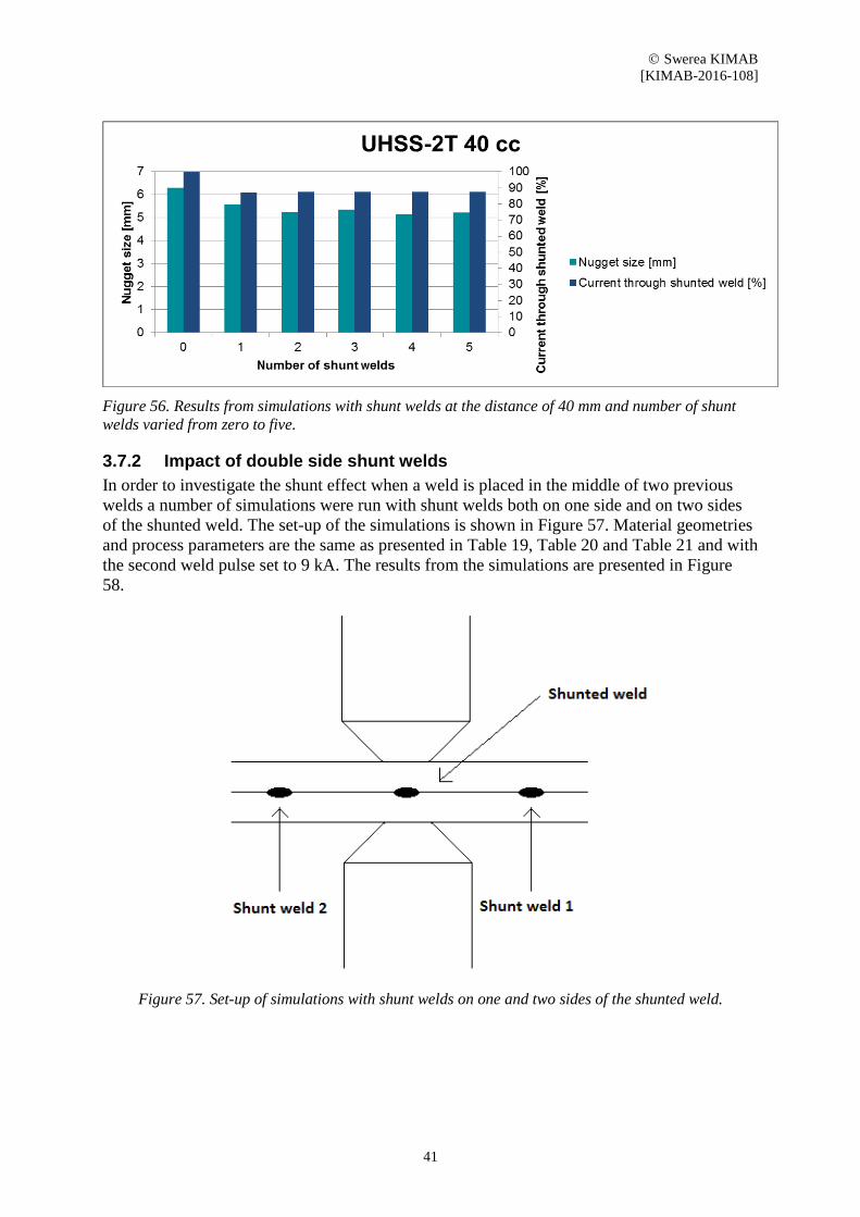
Figure 56. Results from simulations with shunt welds at the distance of 40 mm and number of shunt
welds varied from zero to five.
3.7.2 Impact of double side shunt welds
In order to investigate the shunt effect when a weld is placed in the middle of two previous
welds a number of simulations were run with shunt welds both on one side and on two sides
of the shunted weld. The set-up of the simulations is shown in Figure 57. Material geometries
and process parameters are the same as presented in Table 19, Table 20 and Table 21 and with
the second weld pulse set to 9 kA. The results from the simulations are presented in Figure
58.
Figure 57. Set-up of simulations with shunt welds on one and two sides of the shunted weld.

Swerea KIMAB
[KIMAB-2016-108]
42
Figure 58. Impact on nugget size with shunt welds on both sides of the shunted weld.
3.7.3 Shunt effects in T4 combinations
Tests were also performed to investigate the impact of the distance to the shunt weld in a joint
were a fourth sheet was added to a three-sheet combination. The model were set up as shown
in Figure 59, with a shunt weld placed through three of the four sheets in the combination.
The distance to the shunt weld is varied between 20, 30 and 40 mm. The simulated
combinations are UHSS-4T and HSS-4T. The results from these tests are presented in Figure
60 and Figure 61.
Figure 59. Set-up for simulations with shunt weld through three sheets in four-sheet combination.

Swerea KIMAB
[KIMAB-2016-108]
43
Table 29. Materials and geometries in HSS-4T.
Material Coating Thickness [mm]
Sheet 1 DP600 GI50/50 1.5
Sheet 2 Mild Steel GI50/50 0.7
Sheet 3 Mild Steel GI50/50 0.6
Sheet 4 DP800 GI50/50 1.2
Table 30. Material and geometry for electrodes used in HSS-4T.
Material Geometry
A2/2-Cap B-Cap 20/8
Table 31. Process parameters used in HSS-4T.
Force [kN] 1-Current [kA] 1-time [ms] 1-pause [ms] 2-Current [kA] 2-time [ms]
3.4 11.0 40 0 10.2 510
Figure 60. Impact on nugget size in T4-combination with one shunt weld through three of the four
sheets in UHSS-4T.

Swerea KIMAB
[KIMAB-2016-108]
44
Figure 61. Impact on nugget size in T4-combination with one shunt weld through three of the four
sheets in HSS-4T.
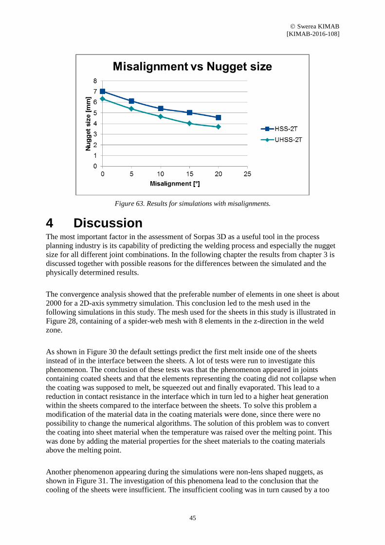
3.8 Misalignments Misaligned sheets and electrodes can be a problem in the process industry. This is a
phenomenon which can occur from angular misalignment or poor fit-up in the sheet-stacks. In
order to investigate the impact of misaligned sheets in the stack-up a number of simulations
were run. The set-up of the simulations is as shown in Figure 62. In order to create the
misalignment, a gap was placed between the sheets at a distance of 25 mm from the weld. The
size of the gap was then varied in order to create different degrees of misalignment. The
nugget size in the test is then compared for different degrees of misalignment. The result is
shown in Figure 63. The simulated cases are HSS-2T and UHSS-3T with the second current
set to 9,9 and 9 kA respectively.
Figure 62. Set-up for misalignment simulations.
Swerea KIMAB
[KIMAB-2016-108]
45
Figure 63. Results for simulations with misalignments.
4 Discussion The most important factor in the assessment of Sorpas 3D as a useful tool in the process
planning industry is its capability of predicting the welding process and especially the nugget
size for all different joint combinations. In the following chapter the results from chapter 3 is
discussed together with possible reasons for the differences between the simulated and the
physically determined results.
The convergence analysis showed that the preferable number of elements in one sheet is about
2000 for a 2D-axis symmetry simulation. This conclusion led to the mesh used in the
following simulations in this study. The mesh used for the sheets in this study is illustrated in
Figure 28, containing of a spider-web mesh with 8 elements in the z-direction in the weld
zone.
As shown in Figure 30 the default settings predict the first melt inside one of the sheets
instead of in the interface between the sheets. A lot of tests were run to investigate this
phenomenon. The conclusion of these tests was that the phenomenon appeared in joints
containing coated sheets and that the elements representing the coating did not collapse when
the coating was supposed to melt, be squeezed out and finally evaporated. This lead to a
reduction in contact resistance in the interface which in turn led to a higher heat generation
within the sheets compared to the interface between the sheets. To solve this problem a
modification of the material data in the coating materials were done, since there were no
possibility to change the numerical algorithms. The solution of this problem was to convert
the coating into sheet material when the temperature was raised over the melting point. This
was done by adding the material properties for the sheet materials to the coating materials
above the melting point.
Another phenomenon appearing during the simulations were non-lens shaped nuggets, as
shown in Figure 31. The investigation of this phenomena lead to the conclusion that the
cooling of the sheets were insufficient. The insufficient cooling was in turn caused by a too
Swerea KIMAB
[KIMAB-2016-108]
46
small contact area between the sheets and the electrodes. In order to increase the contact area
between the sheets, the flow stress curves were modified as shown in Figure 23, Figure 24,
Figure 25 and Figure 26. The study of the material properties did also lead to modifications in
thermal conductivity, specific heat capacity and resistivity as shown in Figure 20, Figure 21
and Figure 22. The new material properties resulted in a process as illustrated in Figure 32.
The new data for these four material properties are those listed as literature and calculated
data in chapter 2.4. These were used in the following simulations in this work.
The investigation of the impact of the material properties showed that the resistivity for the
materials has the highest impact on the result. However, the thermal conductivity and the flow
stress curves do also have a high influence on the result, while the specific heat capacity has a
minor impact on the result. As mentioned in chapter 2.4.1, there are more accurate methods to
examine the thermal conductivity. This method is also possible to use in order to examine the
resistivity and the specific heat capacity of the materials in order to further improve the results
from the simulations.
A number of 1D-lobes were created and compared to physically conducted results of the same
joints in order to investigate the accuracy of the software and to examine its usefulness as a
tool in the process planning industry. As shown in chapter 3.4 the trend in the results is that
the simulations predict a smaller nugget size than the physical testing procedure.
Due to the differences between the simulated and the physical results comparisons between
the resistances in the systems were done. Since the resistance has a major impact on the
generated heat, and in turn on the nugget size, investigations were conducted to compare the
total resistances in the simulations to the total resistance in the physical tests. As illustrated in
Figure 46 and Figure 47 the differences between the two cases have to be considered too
small to cause the differences in nugget size. To further investigate the differences, cross
section comparisons were conducted. This was due to the fact that the simulations showed the
weld size as the melted mean diameter at the interface while the physical testing shows the
weld size as the mean diameter of the peeled nugget. As illustrated in Figure 48, Figure 49,
Figure 50, Figure 51 and Figure 52, the difference between the simulations and the cross-
section tests are within the range of 0,1-0,2 mm, while the differences between the
simulations and the peeled weld size is between 0,8-1 mm. This indicates that the simulations
with the new material data correspond to the physical tests. This agreement indicates that
Sorpas 3D could be useful in the process planning industry in the future.
To examine the impact of shunt effects a number of tests were conducted. Since shunt welds
can exist in a high amount of formations different set-ups were investigated. The set-up in
chapter 3.7.1 evaluated the impact of distance to shunt welds and the impact of number of
shunt welds placed in a sequence. As seen in Figure 54, Figure 55 and Figure 56 the distance
to the shunt weld has a higher impact than the number of shunt welds in the sequence. As
illustrated in Figure 58 the nugget size of the shunted weld decreases when it is placed in the
middle of two previous welds compared to when the welds are placed in sequence. The
investigation with a shunt weld through three out of four sheets in a joint shows that the shunt
weld has a minor effect on the nugget size in the unshunted interface while the influence on
the shunted interfaces follows the same trend as shown in chapter 3.7.1 with decreased nugget
size with decreased distance to the shunt weld.

Swerea KIMAB
[KIMAB-2016-108]
47
In order to investigate the impact of misaligned sheets in a joint two different two-sheet-
combinations were simulated with one of the sheets misaligned. As illustrated in Figure 63,
the weld size decreases with increased degree of misalignment.
To examine the accuracy of the simulations with shunt welds and misaligned sheets
comparisons with physical tests must be conducted. The tests in this study are mainly
conducted in order to investigate how the software treats shunt welds and how to best set up a
model for simulations with misalignments.
5 Conclusions Considering the correspondence between the simulations and the physical tests in the cross-
section comparisons, Sorpas 3D could be useful as a tool in the process planning industry in
the future. However, more studies with different materials and geometries are required to
further establish the agreement. There are also still a number of features in the software which
are missing or needs to be corrected. In order to complement the physical testing the software
needs to be able to predict expulsion. In order to give a good indication of the expulsion limit
a number of factors must be considered. Sorpas 2D has set the expulsion limit to the point
where the molten material comes in contact with the surrounding, however, factors such as
increased pressure in the molten material must also be taken into account. The fact that a
number of modifications in the material database were needed in order to get accurate results
must also be considered before introducing Sorpas 3D into the process planning industry.
Considering the possibility that the problems with the software could be solved with updates
of the material database, a new model concerning the coating elements and with the
implementation of an expulsion criterion, Sorpas 3D possibly could be a useful tool in the
industry. With these additions to the software it could be used in the investigation of
optimized process parameters for new joints. However the nugget size demands must be
updated to fit the weld size given from the simulated results rather than the one from the peel
tests. The user-friendly interface is an advantage in Sorpas 3D which would ease the
implementation of the software.
6 Future work In order to fully investigate the accuracy of Sorpas 3D more studies are required regarding the
differences between the peeled nugget sizes and the cross-section weld sizes for a number of
different combinations. It is also of great importance to examine a functioning expulsion
criterion in order to optimize the welding parameters and to create 1D-lobes for new joints.
7 Acknowledgments First I would like to thank my supervisor at Swerea KIMAB AB, Johannes Gårdstam, for his
great support and guidance through this work and for providing of extensive knowledge both
within the field of resistance welding and the field of simulations. I would also like to thank

Swerea KIMAB
[KIMAB-2016-108]
48
Oscar Andersson at KTH Royal Institute of Technology for his help during this work and for
always answering all of my questions. I would also like to thank Professor Arne Melander at
Swerea KIMAB AB for guidance and good discussions. Thanks also to Gert Larsson and
Johnny K. Larsson at Volvo Cars for good inputs, guidance and providing me with
understanding in industrial use. I would also like to thank my supervisor at KTH Royal
Institute of Technology Professor Per-Lennart Larsson for his support during this work.
Thanks also to Mats Danielsson, Paul Janiak, Kjell-Arne Persson, Joakim Hedegård, Marie
Allvar and Miroslava Sedlakova at Swerea KIMAB AB for their help, guidance and for
fruitful discussions during my work. I would also like to thank Sune Evertsson at Volvo Cars
for providing me with data and for good discussions regarding testing and quality inspection.

Swerea KIMAB
[KIMAB-2016-108]
49
8 References
[1] K. Weman, Karlebo Svetshandbok,
Stockholm: Liber AB, 2013.
[2] H. Zhang and J. Senkara, Resistance
Welding: Fundamentals and
Applications, Boca Raton: CRC Press,
2006.
[3] O. Andersson, "Process planning of
resistance spot welding," KTH,
Stockholm, 2013.
[4] N. Harlin, T. B. Jones and J. D.
Parker, "Weld growth mechanisms
during resistance spot welding of two
and three thickness lap joints,"
Science and Technology of Welding
and Joining, vol. 7, no. 1, pp. 35-41,
2002.
[5] J. Gårdstam och O. Skrinjar,
”Simulation of spotwelding - a
literature review,” Korrosions och
metallforskningsinstitutet (KIMAB),
Stockholm, 2006.
[6] B. Wang, M. Lou, Q. Shen, Y. B. Li
and H. Zhang, "Shunting effect in
Resistance Spot Welding Steels - Pars
1: Experimental Study," Welding
Journal, vol. 92, pp. 182-189, 2013.
[7] H. S. Chang och H. S. Cho, ”A Study
on the Shunt Effect in Resistance Spot
Welding,” Welding Journal, vol. 69,
nr 8, pp. 308-317, 1990.
[8] Q. Song, ”Testing and Modeling of
Contact Problems in Resistance
Welding,” Technical University of
Denmark, Kgs. Lyngby, 2003.
[9] M. Hasir, ”A study of the Peltier
effect in the resistance spot welding of
very thingage sheet electroplated with
tin using tungsten electrodes,”
Welding and Cutting, vol. 36, nr 3, pp.
116-121, 1984.
[10] S. Fukumoto, I. Lum, E. Biro, D. R.
Boomer och Y. Zhou, ”Effects of
electrode degradation on electrode life
in resistance spot welding of
aluminum alloy 5182,” Welding
journal - New York, vol. 82, nr 11, pp.
307-312, 2003.
[11] K. Zhou och L. Cai, ”Study on effect
of electrode force on resistance spot
welding process,” Journal of Applied
Physics, vol. 116, nr 8, 2014.
[12] ISO 5182:2008 Resistance welding -
Materials for electrodes and ancillary
equipment.
[13] ISO 5821:2009 Resistance Welding -
Spot welding electrode caps.
[14] J. D. Parker, N. T. Williams och R. J.
Holliday, ”Mechanisms of electrode
degradation when spot welding coated
steels,” Science and Technology of
Welding and Joining, vol. 3, nr 2, pp.
65-74, 998.
[15] W. D. Callister och D. G. Rethwisch,
Materials Science and Engineering,
Eight Edition, New York: Wiley,
2011.
[16] Y. Sakuma och H. Oikawa, ”Factors
to determine static strengths of spot-
weld for high-strength steel sheets and
developments of high-strength steel
sheets with strong and stable welding
characteristics,” Shinnittetsu Giho,
2003.
[17] SS-EN ISO 14373:2015 Resistance
welding - Procedure for spot welding
of uncoated and coated low carbon
steels.
[18] SS-EN ISO 10447:2007 Resistance
welding - Peel and chisel testing of
resistance spot and projection welds.
[19] J. Senkara och H. Zhang, ”Cracking in
spot welding aluminum alloy
AA5754,” Welding Journal, vol. 79,
nr 7, pp. 194-201, 2000.
[20] A. Runnemalm och A. Appelgren,
”Evaluation of non-destructive testing
methods for automatic quality
Swerea KIMAB
[KIMAB-2016-108]
50
checking of spot welds,” University
West.
[21] M. Thornton, L. Han and M.
Shergold, "Progress in NDT of
resistance spot welding of aluminum
using ultrasonic C-scan," NDT&E
International, vol. 48, pp. 30-38,
2012.
[22] SS-EN ISO 14327:2004 Resistance
welding - Procedures for determening
the weldability lobe for resistance
spot, projection and seam welding.
[23] VCS 8631, 16 Weldability of sheet
metal, spot welding.
[24] C. V. Nielsen, P. A. F. Martins, W.
Zhang och N. Bay, ”Numerical
methods in simulation of resistance
welding,” i 6th International
Conference on Computational
Methods for Coupled Problems in
Science and Engineering, 2015.
[25] Z. Han, J. Orozco, J. E. Indacochea
och C. H. Chen, ”Resistance Spot
Welding: A Heat Transfer Study,”
Welding Journal, vol. 68, pp. 363-
371, 1989.
[26] H. A. Neid, ”The Finite Element
Modeling of the Resistance Spot
Welding Process,” Welding Journal,
vol. 63, pp. 123-132, 1984.
[27] C. L. Tsai, W. L. Dai, D. W.
Dickinson och J. C. Papritan,
”Analysis and Development of a Real-
Time Control Methodology in
Resistance Spot Welding,” Welding
Journal, vol. 70, pp. 339-351, 1991.
[28] C. V. Nielsen och W. Zhang, ”3D
simulation of Resistance Welding
Processes and Weld Strength
Testing,” i Simulationsforum 2013:
Schweissen und Wärmebehandlung,
Weimar, 2013.
[29] J. Gårdstam, ”Temperature dependent
material properties of HSS sheets used
for welding simulations,” Swerea
KIMAB AB, Stockholm, 2008.
[30] Z. Hou, I.-S. Kim, Y. Wang, C. Li och
C. Chen, ”Finite element analysis for
the mechanical features of resistance
spot welding process,” Journal of
Materials Processing Technology,
vol. 185, pp. 160-165, 2007.
[31] J. Saleem, A. Majid, K. Bertilsson, T.
Carlberg och N. Ul Islam, ”Nugget
Formation During Resistance Spot
Welding Using Finite Element
Model,” World Academy of Science,
Engineering and Technology: An
International Journal of Science,
Engineering and Technology, vol. 67,
2012.
[32] W. Zhang, ”Design and
Implementation of Software for
Resistance Welding Process
Simulations,” Journal of Materials
and Manufacturing, vol. 112, nr 5, pp.
556-564, 2003.
[33] C. V. Nielsen, W. Zhang, L. M.
Alves, N. Bay och P. Martins,
Modeling of thermo-electro-
mechanical manufacturing processes:
applications in metal forming and
resistance welding, Springer Science
and Buisness Media, 2012.
[34] S. Min, J. Blumm och A. Lindemann,
”A new laser flash system for
measurement of the thermophysical
properties,” Thermochimica Acta, vol.
455, pp. 46-49, 2007.

www.kth.se