3D Analyst: An IntroductionJinwu Ma

Khalid Duri

▪ What’s New

▪ 3D Data Types

▪ LAS & Surface Analysis

▪ 3D Feature Analysis

▪ Demos

▪ Q & A

Workshop Outline

What’s New

▪ Improved depth enhancement for LAS visualization

▪ Improved results & performance for Classify LAS Building

▪ Improved performance for Polygon Volume calculation

▪ Clip 3D line profile graph to visible extent

▪ Easily add multiple surfaces as separate elevation sources

▪ Generate a profile view to interactively examine a 3D cross section

▪ Interactively assess the cut-fill needed to level an elevation surface

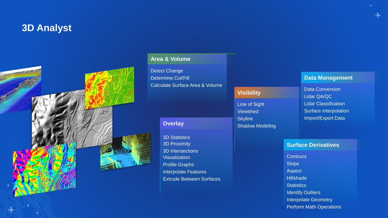
3D Analyst

Contours

Slope

Aspect

Hillshade

Statistics

Identify Outliers

Interpolate Geometry

Perform Math Operations

Detect Change

Determine Cut/Fill

Calculate Surface Area & Volume

3D Statistics

3D Proximity

3D Intersections

Visualization

Profile Graphs

Interpolate Features

Extrude Between Surfaces

Line of Sight

Viewshed

Skyline

Shadow Modeling

Data Conversion

Lidar QA/QC

Lidar Classification

Surface Interpolation

Import/Export Data

Surface Derivatives

Area & Volume

Overlay

Visibility

Data Management

Surface Types & Vector Geometry

Overview of 3D Data Types

Storing XYZ Information

Vector Geometry

Points | Lines| Polygon

Point Cloud

Multipatch | Mesh

Triangulated Irregular Network

Raster

Surface Model

Understanding the 3D Mesh

▪ Collection of triangles that define 3D shapes

▪ Support textures, colors, and transparency

▪ Can be used to represent many types of data:

¬ Discrete objects

Ͱ Buildings

Ͱ Vegetation

Ͱ Machinery

¬ Continuous measurements

Ͱ Terrain

Ͱ Volumetric shells

Multipatch Geometry

▪ Native mesh geometry format for ArcGIS

▪ Supports textures & colors when stored in a geodatabase

▪ Supported as input for numerous

automated analysis operations

▪ Single resolution dataset

▪ Created by:

¬ Editing in ArcGIS Pro

¬ Deriving from surfaces

¬ Importing from other 3D model formats

¬ Symbolizing points, lines, and polygons

with 3D properties

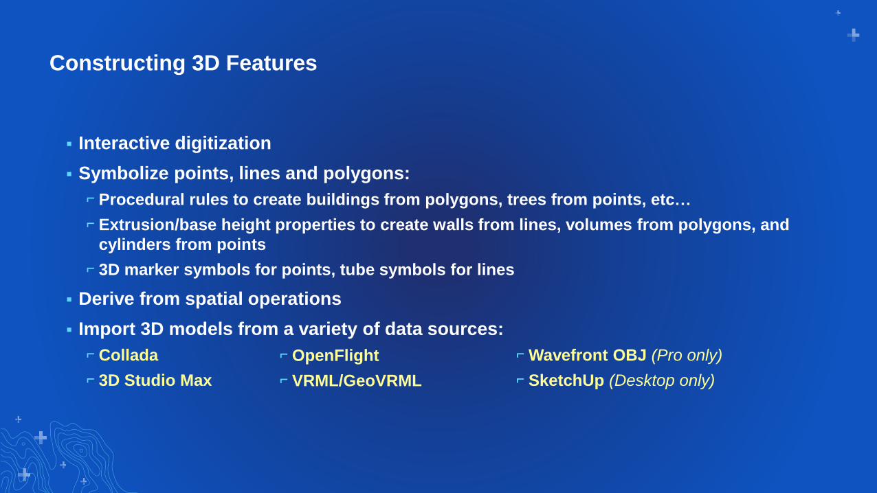
Constructing 3D Features

▪ Interactive digitization

▪ Symbolize points, lines and polygons:

⌐ Procedural rules to create buildings from polygons, trees from points, etc…

⌐ Extrusion/base height properties to create walls from lines, volumes from polygons, and

cylinders from points

⌐ 3D marker symbols for points, tube symbols for lines

▪ Derive from spatial operations

▪ Import 3D models from a variety of data sources:

⌐ Collada

⌐ 3D Studio Max

⌐ OpenFlight

⌐ VRML/GeoVRML

⌐ Wavefront OBJ (Pro only)

⌐ SketchUp (Desktop only)

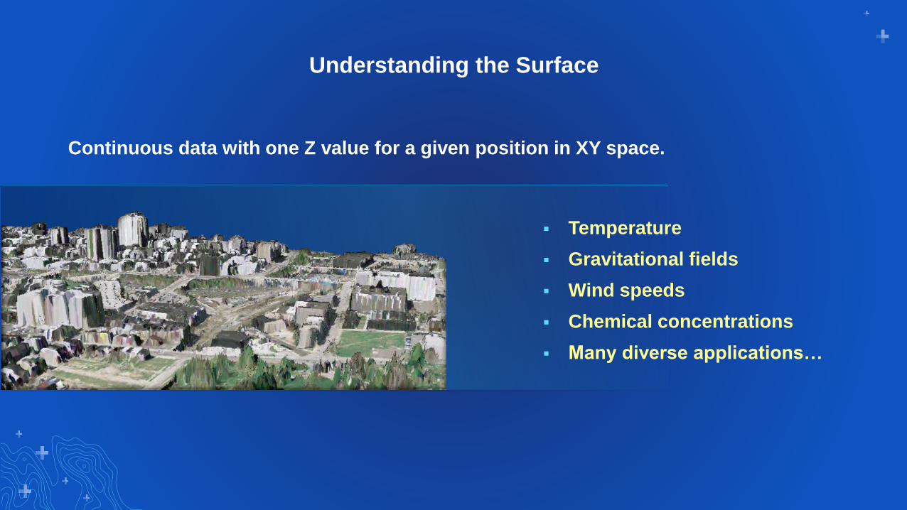
Understanding the Surface

Continuous data with one Z value for a given position in XY space.

▪ Temperature

▪ Gravitational fields

▪ Wind speeds

▪ Chemical concentrations

▪ Many diverse applications…

Surface Data Models

Raster Surface

TIN Based Surfaces

- Made by interpolation, generalize source measurements

to cell size

- Fast to process, support robust math operations

- Created by triangulation, maintain source measurements

- Support robust surface definitions & data

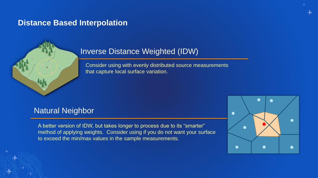
Distance Based Interpolation

Inverse Distance Weighted (IDW)

Consider using with evenly distributed source measurements

that capture local surface variation.

Natural Neighbor

A better version of IDW, but takes longer to process due to its “smarter”

method of applying weights. Consider using if you do not want your surface

to exceed the min/max values in the sample measurements.

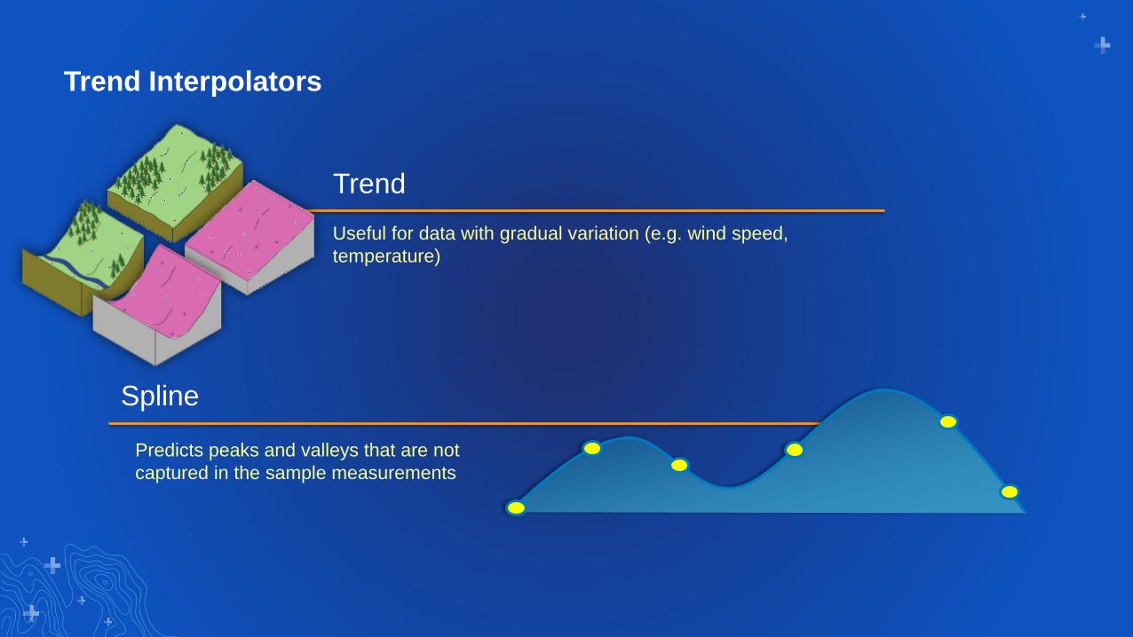
Trend Interpolators

Trend

Useful for data with gradual variation (e.g. wind speed,

temperature)

Spline

Predicts peaks and valleys that are not

captured in the sample measurements

Geostatistical & Geomorphological Interpolation

Kriging

Consider using with evenly distributed source measurements

that capture local surface variation.

Topo To Raster

Creates hydrologically correct surface that eliminates local sinks, designed

to work well with contour lines

Se

miv

ar

ia

nc

e

Distance

Empirical Semivariogram

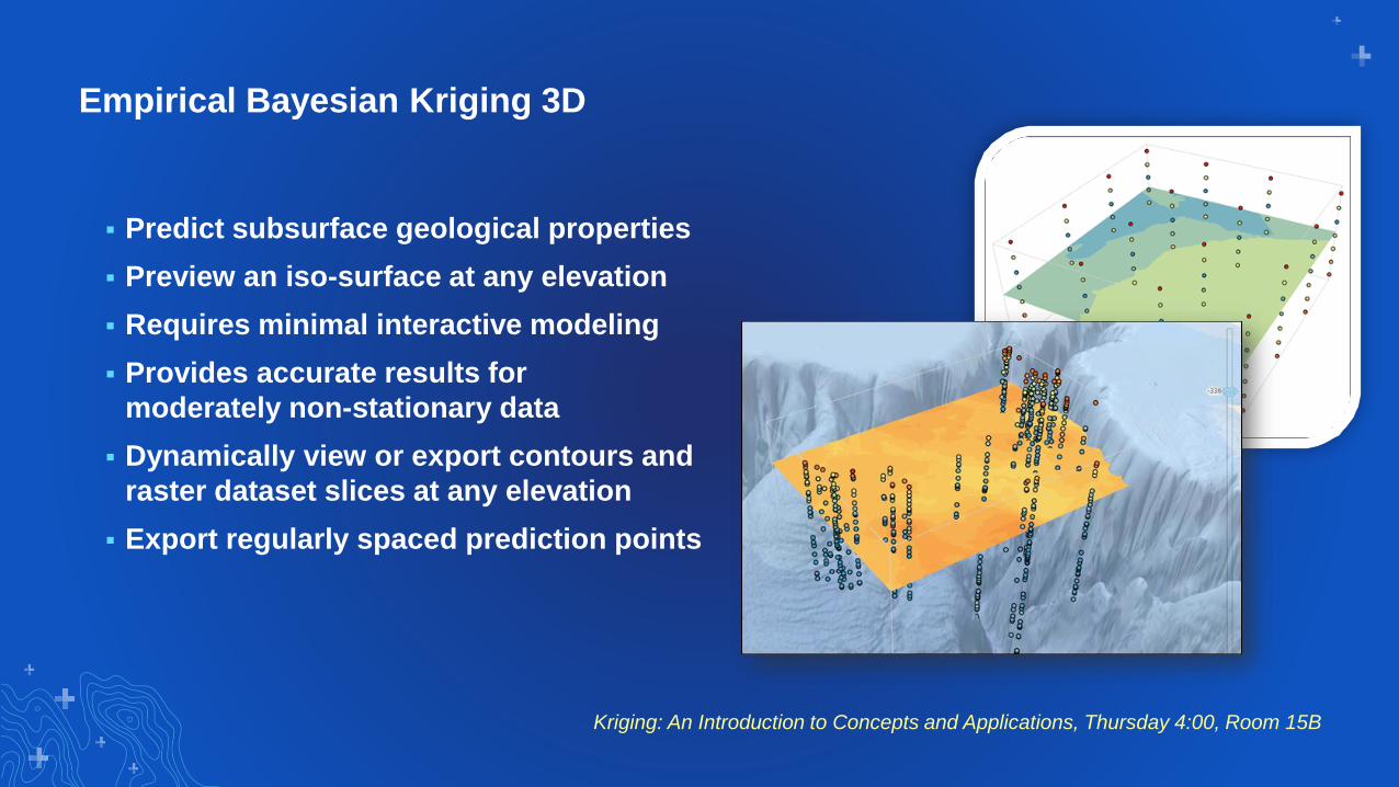
Empirical Bayesian Kriging 3D

▪ Predict subsurface geological properties

▪ Preview an iso-surface at any elevation

▪ Requires minimal interactive modeling

▪ Provides accurate results for

moderately non-stationary data

▪ Dynamically view or export contours and

raster dataset slices at any elevation

▪ Export regularly spaced prediction points

Kriging: An Introduction to Concepts and Applications, Thursday 4:00, Room 15B

Triangulated Irregular Network (TIN) Surfaces

TIN

Terrain

LAS Dataset

Well-suited for engineering applications and analysis of study areas

that are not exceedingly large, provides interactive editing options.

Multi-resolution, scalable, offers robust support for handling large

amounts of data.

Rapidly visualize, filter, perform QA/QC and analyze lidar data. Well

suited for aerial collections, supports compressed lidar in ZLAS format.

Surface Feature Types

Also supports:

▪ Break lines

▪ Tag values

▪ Mass points: Measurements

used for triangulation

▪ Erase polygon: Interior areas of

no data

▪ Replace polygon: Assigns a

constant z value

▪ Clip polygon: Defines the

interpolation zone

Hard & Soft Edges

TIN Editing Toolbar in ArcMap

TIN Editors: Add, modify, or remove nodes, edges, triangles & tag values

Grading Tool: Modify

surface using line with

slope properties.

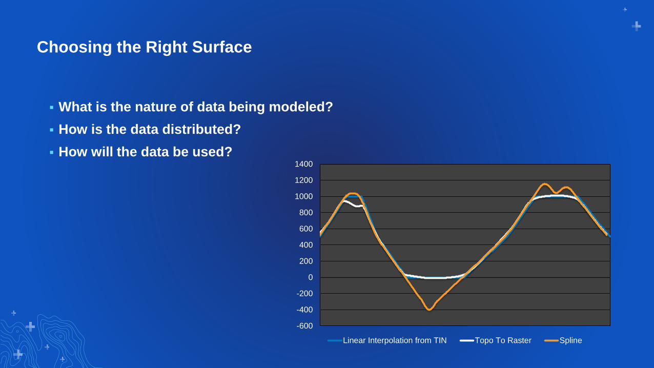
Choosing the Right Surface

▪ What is the nature of data being modeled?

▪ How is the data distributed?

▪ How will the data be used?

-600

-400

-200

0

200

400

600

800

1000

1200

1400

Linear Interpolation from TIN Topo To Raster Spline

Classification | Spatial Statistics | Surface Derivatives

LAS & Surface Analysis

Surface Analysis

▪ Change detection

▪ Calculate area & volume

▪ Proximity analysis

▪ Robust mathematical operations

▪ Surface derivatives

⌐ Slope

⌐ Curvature

⌐ Aspect

⌐ Contour Lines

LAS Analysis

▪ Automated classification support:

⌐ Ground

⌐ Building

⌐ Noise

▪ Proximity analysis

▪ Point statistics

▪ Surface derivatives

⌐ Overlap scans

⌐ Height above ground

⌐ Proximity to 2D/3D Features

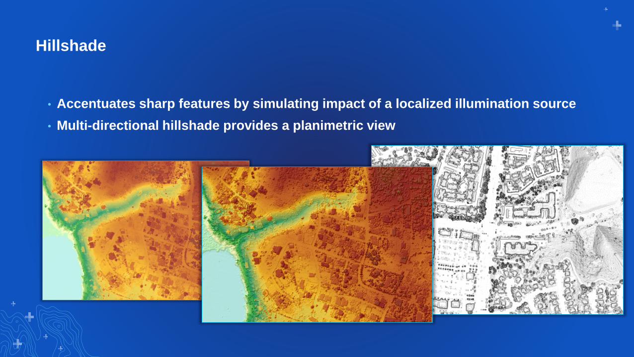
Hillshade

• Accentuates sharp features by simulating impact of a localized illumination source

• Multi-directional hillshade provides a planimetric view

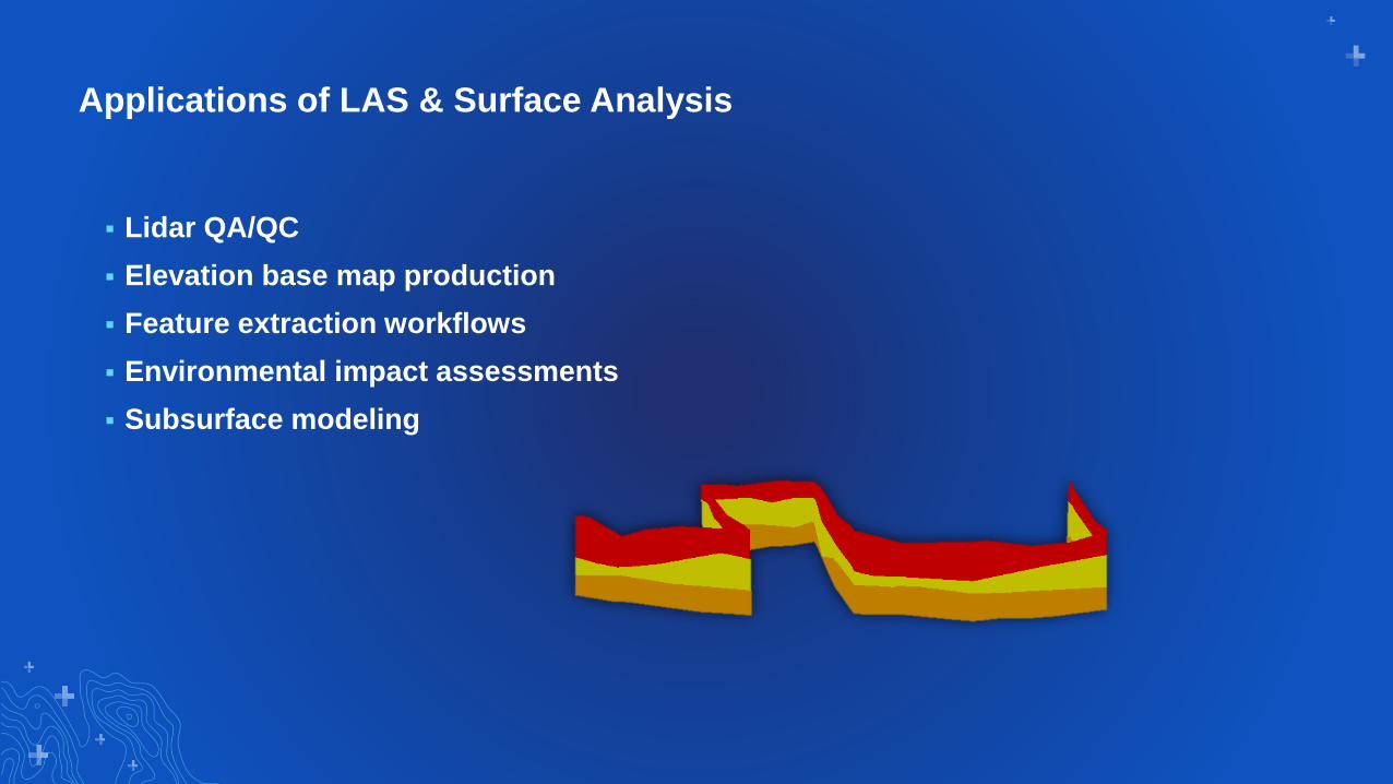
Applications of LAS & Surface Analysis

▪ Lidar QA/QC

▪ Elevation base map production

▪ Feature extraction workflows

▪ Environmental impact assessments

▪ Subsurface modeling

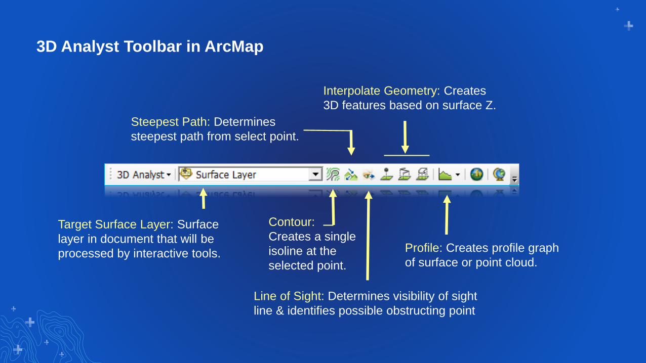
3D Analyst Toolbar in ArcMap

Steepest Path: Determines

steepest path from select point.

Target Surface Layer: Surface

layer in document that will be

processed by interactive tools.

Contour:

Creates a single

isoline at the

selected point.

Line of Sight: Determines visibility of sight

line & identifies possible obstructing point

Interpolate Geometry: Creates

3D features based on surface Z.

Profile: Creates profile graph

of surface or point cloud.

Overlay | Proximity | Visibility

3D Feature Analysis

Proximity Analysis

▪ Create 3D buffers

▪ Identify closest objects

▪ Find intersection of 3D lines with surfaces & multipatch shapes

▪ Construct the minimum bounding volume encompassing a cluster of points

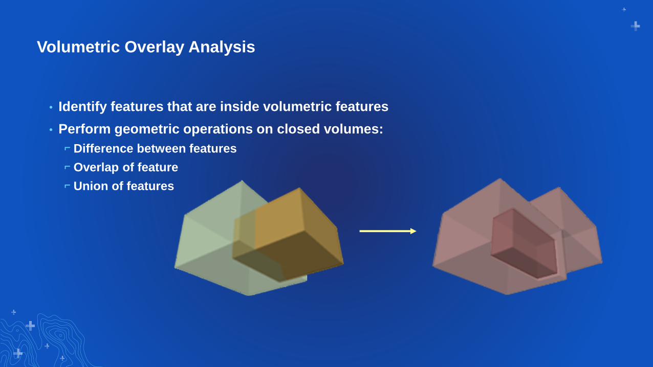
Volumetric Overlay Analysis

• Identify features that are inside volumetric features

• Perform geometric operations on closed volumes:

⌐ Difference between features

⌐ Overlap of feature

⌐ Union of features

Applications of 3D Feature Analysis

▪ Asset management

▪ Clearance/safety assessment

▪ Subsurface visualization & analysis

▪ Assessing the impact and interaction of built structures

▪ Modeling volumetric shells for thresholds of continuous data

▪ Preparing visualization for web/mobile

Section Subhead

Visibility Analysis

Controlling the Observer

Viewshed frustum defined by:

▪ Azimuth & vertical angle range

▪ Visible distance range

▪ Observer and target offset

0°

90°

180°

270°Min

Distance

MaxDistance

45°

-45°

90°

-90°

0°

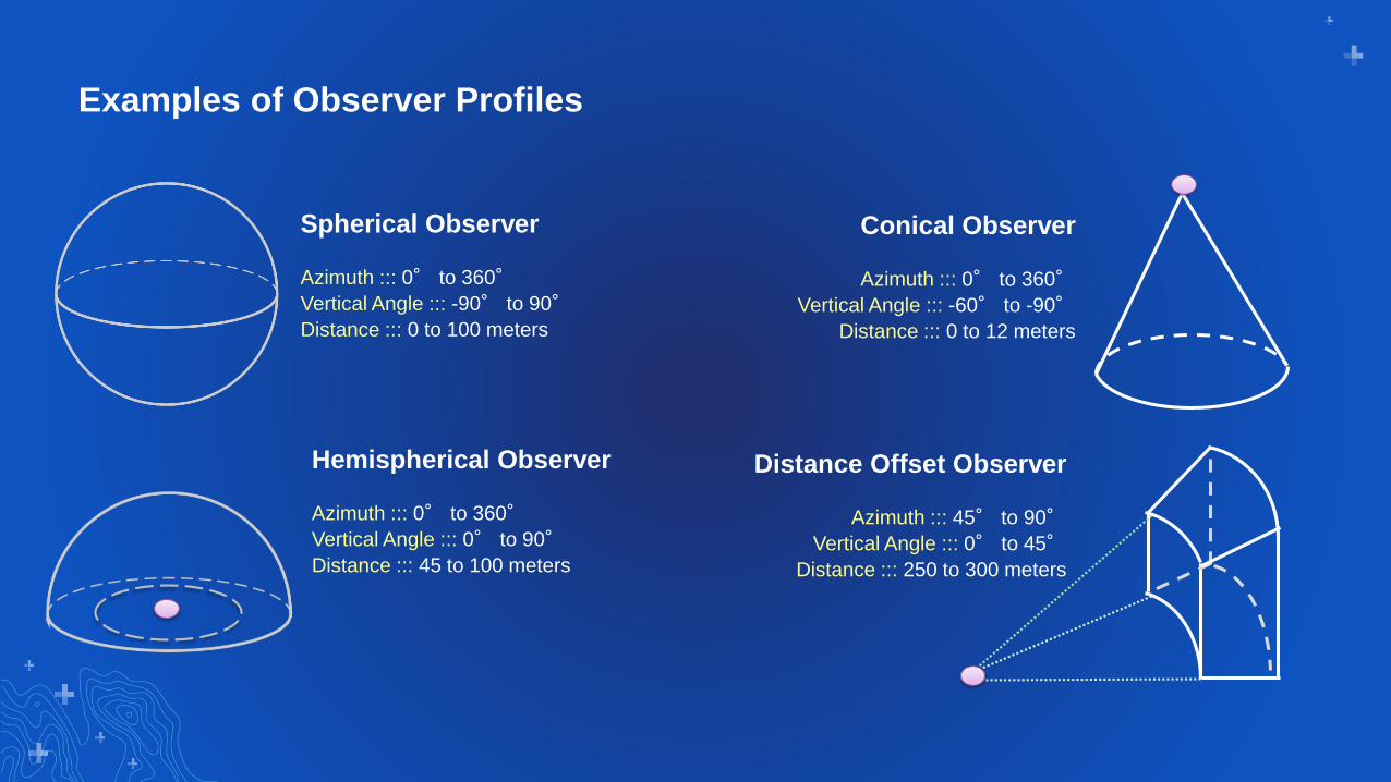
Examples of Observer Profiles

Spherical Observer

Azimuth ::: 0° to 360°

Vertical Angle ::: -90° to 90°

Distance ::: 0 to 100 meters

Hemispherical Observer

Azimuth ::: 0° to 360°

Vertical Angle ::: 0° to 90°

Distance ::: 45 to 100 meters

Conical Observer

Azimuth ::: 0° to 360°

Vertical Angle ::: -60° to -90°

Distance ::: 0 to 12 meters

Distance Offset Observer

Azimuth ::: 45° to 90°

Vertical Angle ::: 0° to 45°

Distance ::: 250 to 300 meters

Atmospheric Refraction

▪ Bending of light passing through the atmosphere

▪ Influenced by variations in air pressure, density, humidity, temperature & elevation

▪ Refraction coefficient supported in:

Ͱ Line of Sight

Ͱ Skyline

Ͱ Viewshed

Ͱ Solar Radiation

Sightline Analysis

• Visibility along 2-vertex line in 3D space

• Identify obstruction point

• Interactively generate and manipulate a

sightline for exploratory analysis

Skyline Analysis

▪ Segment the horizon by its contributing features

▪ Create closed volumes bounded by the skyline

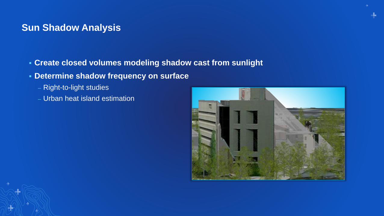
Sun Shadow Analysis

▪ Create closed volumes modeling shadow cast from sunlight

▪ Determine shadow frequency on surface

— Right-to-light studies

— Urban heat island estimation

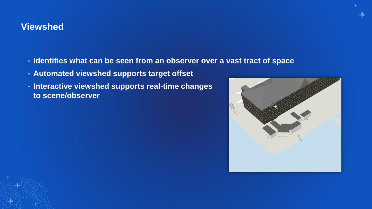
Viewshed

• Identifies what can be seen from an observer over a vast tract of space

• Automated viewshed supports target offset

• Interactive viewshed supports real-time changes

to scene/observer

Using Exploratory & Automated

Tools

3D Analysis Demos

Please Share Your Feedback in the App

Download the Esri

Events app and find

your event

Select the session

you attended

Scroll down to

“Survey”

Log in to access the

survey

Complete the survey

and select “Submit”