394 adaptive control full penetration gas tungsten …ymzhang/papers/ieee control systems...394 ieee...

394 IEEE TRANSACTIONS ON CONTROL SYSTEMS TECHNOLOGY, VOL. 4, NO. 4, JULY 1996

Adaptive Control of Full Penetration Gas Tungsten Arc Welding

Yu M. Zhang, Radovan Kovacevic, and Lin Li

Abstruct- This application paper addresses the control of a nonminimum-phase plant with variable large orders and delays. The process concerned is full penetration gas tungsten arc welding. Based on an analysis of accepted adaptive algorithms, the generalized predictive control algorithm presented by Clarke et al. is selected as the principal control strategy. An adaptive generalized predictive decoupling control scheme is constructed. To decouple our nonminimum-phase multivariable plant, a predictive decoupling algorithm is also proposed. Simulations are performed to determine the default parameters of the algorithms. The performance has been tested by both simulations and experiments.

I. INTRODUCTION EAM tracking and weld penetration control are two fundamental issues in automated welding. A number of

approaches, including pool oscillation, infrared sensing, ul- trasonic sensing, and radiography, have been proposed to sense the weld penetration from the weld-face [ 1 I . Whereas the seam tracking technology has matured, however, accurate penetration control still remains an unresolved problem due to the limitations associated with each individual sensing method. New sensing principles are strongly needed [l]. It is known that the sag depression is directly determined by the geometry of the pool bottom surface. Thus, we proposed to monitor the full penetration state, which is specified by the backside bead width, using the geometry of the sag behind the pool rear. Experimentation showed that despite variations in the welding conditions and parameters, the backside bead width can be accurately determined from the sag depression using a simple linear model [l]. This reflects the inherent dependence of the sag geometry on the backside opening. It is known that the weld penetration status is essential in the root pass. To acquire high quality joints, the root pass is frequently gas tungsten arc (GTA) welded. The above correlation was acquired based on GTA welding without filler. Thus, this correlation can be used to develop a practical penetration control method, with a weld-face sensor that can be attached to and move with the torch.

To control the full penetration using the sag depression, a laser stripe was projected onto the sag behind the weld pool. A real-time image processing algorithm was developed.

Manuscript received April 5, 1995; revised January 19, 1996. Recom- mended by Associate Editor, E. 0. King.

The authors are with the Center for Robotics and Manufacturing Systems, University of Kentucky, Lexington, KY 40506 USA.

Publisher Item Identifier S 1063-6536(96)04927-5.

Despite the arc and slag, the sag geometrical parameters can be accurately acquired in real-time [2]. Also, the GTA welding process has been analyzed to provide process characteristics and a model for the control design [3]. In this study, the welding process is referred to as the full-penetration process (FPP) because our goal is to control the backside bead width of a fully penetrated joint.

It has been shown that the FPP is nonminimum phase with variable large orders and delays [3]. Due to the short welding duration, only a few key parameters can be realistically identified on-line rather than all the model parameters, orders and delays. Thus, inexact orders and delays will have to be addressed, and consequently, the conventional adaptive algorithms such as the generalized minimum variances (GMV) or pole-placement will probably fail if applied to our problem. For example, the GMV performs poorly if the plant delay varies [4], even if it is robust with respect to our assumed model order. Other approaches [SI which attempt to estimate the delays using operating data tend to be complex and lack robustness. Unless special precautions are taken, pole- placement and the linear quadratic Gaussian (LQG) self-tuner are sensitive to the overestimation of the model order due to the poleizero cancellations in the identified model [4]. The possibility of applying a multivariable proportional integral derivative (PID) or fuzzy controller was also investigated through simulations. Their performance in terms of trade- off between the response speed and overshooting was not satisfactory. Because of the uncertain delay, the H , controller is difficult to apply [6]. The generalized predictive control (GPC) presented by Clarke et al., however, has been shown to be capable of effective control of a plant with simultaneous variable delay, variable order and nonminimum-phase as well as open-loop unstable properties. This algorithm has been successfully used to control the area of the weld pool [7].

An adaptive predictive decoupling control scheme, utilizing GPC as the essential control strategy, is proposed for the FPP. A V-predictive hybrid decoupling element is incorporated to decouple the coupled nonminimum-phase plant. Simulations are performed to determine default algorithm parameters and examine the system performance. Welding experiments under a wide variety of welding conditions and disturbances are also conducted. It is shown that the desired sag geometry can be achieved despite the variations in the welding conditions.

11. BACKGROUND

The cross section of a fully penetrated joint can be described by Fig. 1. In general, the sag depression depth H , the sag

1063-6536/96$05.00 0 1996 IEEE

ZHANG et al.: ADAPTIVE CONTROL OF FULL PENETRATION GTA WELDING 395

I

b b

Fig. 1. Full penetration weld parameters. This is a cross section of a full penetration weld. S is the cross section area of the sag depression, b is the sag width. The average sag depression h is defined as the ratio h = S /b .

+ ho, bo (set-points)

Fig. 2. laser, lens, and camera, is attached to and moves with the torch.

Experimental system diagram. The sensor, which consists of the

width b, and the backside bead width b b are used to describe the cross section geometrically. It was observed that when H and b were utilized to describe bb , no adequate relationship could be found. Thus a new geometric parameter, called the average sag depression depth, is defined by h = S/b where S is the sag depression area (see Fig. 1). It was found that bb

can be determined with sufficient accuracy by h [l]. The sag geometry was measured by a vision system (Fig. 2) .

A laser stripe was projected onto the sag behind the pool rear. The measurement accuracy of the sag geometry is determined by the image signal-noise ratio, resolution and processing technique. The signal-noise ratio increases when the distance between the pool rear and laser stripe increases, for a certain optical filter and laser. A larger distance, however, will produce a larger delay for the weld penetration control. A trade-off between the image processing and the delay must be considered. Experiments have shown that a satisfactory performance of image processing can be guaranteed if the distance from the pool rear to the stripe is not less than 5 mm. Thus, the laser stripe was selected to be 20 mm behind the electrode. For this sensor configuration, an image processing algorithm has been proposed to reliably acquire the sag geometrical parameters in real-time [2]. The sag parameters h and b are measured using the sensor resolutions along the depression direction (pixel, = 0.0436 mm) and along the pool width direction (pixel, = 0.05 mm), respectively.

A typical GTA welding speed, 2 mm per second, is used in the control experiments. To acquire a fine and smooth full

Fig. 3. Controlled process.

TABLE I NOMINAL MODEL

h(k)-b , , =0.03~4i(k-9-1)+0.0107i(k-9-2)+0.0214i(k-9-3) + O.O064i(k - 9 - 4) + 0.0075i(k - 9 - 5 ) + 0.03 18i(k - 9 - 6) + 0.0240i(k - 9 - 7) + 0.0406i(k - 9 - 8) + 0.0149i(k - 9 - 9) + 0.01:10i(k - 9 -10) + 0.0221i(k - 9 - 11) + 0.0175i(k - 9 - 12)

Model + o . o s T ~ ~ ( ~ - 9 - 13) - 0.3845r(k - 16 - 1) b(k)- b, =0.3641(i(k-15- 1)+0.1819i(k-15-2)+0.16~i(~-~5-3)

+ 0.1632i(k - 15 - 4) + 0.0564i(k - 15 - 5) + 0.2155i(k - 15 - 6) +4.171(1:-16-1)

structure parameters * The aprion values, used as the nominal values, of b,, and b,, are 8.93 and 142.3. In the model, the current and arc length are measured by their differences with 120 A and 3 mm, respectively.

M,, = 13, M,, = 1, M,, =6, M,, = 1 d,, = 9, d,, = 16, d,, = 15, d,, = 16

penetration, the control variables should be adjusted in a small range along the seam. This range is selected to be 1 mm. Thus, the sampling interval !of the control system is 0.5 s. Since the image processing algorithm can acquire the sag parameters in 200 ms [2], there is 300 ms for implementing an adaptive control algorithm.

Although the full penetration is solely determined by h, a uniform sag width, is also required. Thus, both h and b will be controlled as the outputs of the process. The welding current z and arc length 1 are selected as the control variables. The FPP can be described by Fig. 3 where pi j = XiCzl b i j ( k ) ~ - ' - ~ ~ . l (i = 1 , 2 , j = 1,2) [3]. Here bij is the model coefficient, and Mij, and d i j are the suborder and subdelay, respectively. ~1 and E Z are the noises. In the control experiments, bmij, d i j , and Mij will use their values in the nominal model (Table I) and therefore will not be identified on-line. X i ( i = 1, 2) and bio(i = 1, 2) are the on-line adjustable (OLA) parameters that will be identified during welding proces,s control. It can be seen that the process has been described by a moving-average (MA) model, rather than an autoregressive moving-average (ARMA). From the standpoint of decreasing the number of the parameters for on-line estimation in adaptive control, a model with an au- toregression term is preferred. The k-step-ahead prediction accuracy of ARMA models, however, decreases significantly with the prediction step k , whereas the prediction accuracy of a MA model is independlent of the prediction step. In this study,


12

11

8

7 0 5 10 15 20 25

time (second)

(a)

-4

e E

5.

v)

8 9

170

160

150

140

130

120

- individual

0 5 10 15 20 25 time (second)

-25 -20 -15 -10 -5 0 5 10 15 20 25 time (second)

(C)

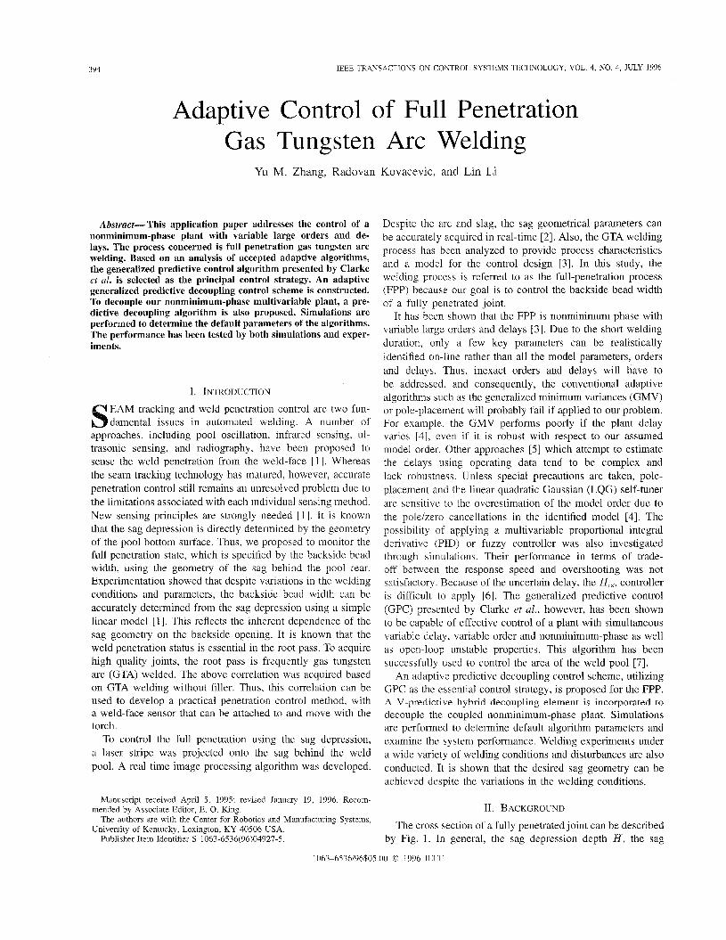
Fig. 4. responses, (c) Step inputs.

Variations in process responses: (a) h step responses, (b) b step

the predictive control needs long-range predictions, therefore MA models were selected [3].

The model parameters, including the coefficients, orders, and delays, vary with the welding conditions. To model the FPP, six typical welding conditions were selected to perform dynamic experiments in our previous study [3] . Six individual models have been fit from each experiment. It was found that the parameters do vary in large ranges. This variation in the model parameters can also be seen from their step responses (Fig. 4). Using all the experimental data, a model has been fit as the nominal model (Fig. 4 and Table I). It has been shown that zeros exist in the nominal model which are outside the unit circle [3]. Thus, the process being addressed is nonminimum phase. The large delay and slow speed of response can also be observed in these step responses.

Ill. CONTROL DESIGN The proposed control architecture is shown in Fig. 5. The

control system consists of four essential parts: 1) plant; 2) estimator; 3) predictive control algorithms; and 4) decoupling elements. The plant is the FPP with the welding current z and arc length 1 as inputs and h and b as outputs [3] . The estimator identifies the OLA parameters based on the inputloutput data. Using the updated OLA parameters and set-points, the predictive control algorithms calculate the generalized welding current i and generalized arc length 1, which are inputs of the decoupling elements. Then, the decoupling elements compute the welding current i and arc length 1, which are actual inputs of the plant, based on the OLA parameters, generalized welding current a, and generalized arc length 1.

S h b

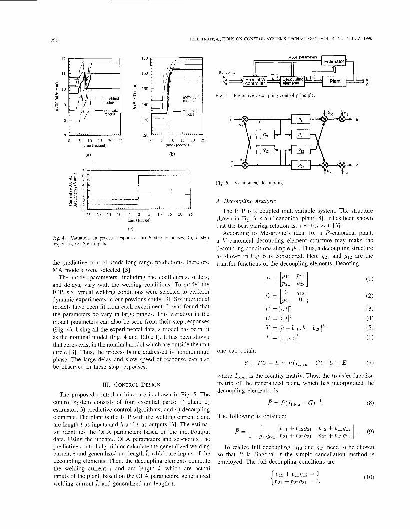
Fig. 5 , Predictive decoupling control principle

1 b

Fig. 6. V-canonical decoupling

A. Decoupling Analysis

The FPP is a coupled multivariable system. The structure shown in Fig. 3 is a P-canonical plant [8]. It has been shown that the best pairing relation is: i - h,Z - b 131.

According to Mesarovic' s idea, for a P-canonical plant, a V-canonical decoupling element structure may make the decoupling conditions simple [8]. Thus, a decoupling structure as shown in Fig. 6 is considered. Here gal and g12 are the transfer functions of the decoupling elements. Denoting

(1)

( 2 )

Pll P12 = [lal ,221

= [g2, 0 1 0 g12

U = [ i , 1 ] t ( 3 ) U = E, iy (4) Y = [h - b l o , b - b20jt ( 5 ) E = [ E l , E 2 I t (6)

one can obtain

Y = PU + E = P ( l l d e n - G)-'U + E (7)

where I1den is the identity matrix. Thus, the transfer function matrix of the generalized plant, which has incorporated the decoupling elements, is

The following is obtained:

To realize full decoupling, g12 and g21 need to be chosen so that p is diagonal if the simple cancellation method is employed. The full decoupling conditions are


Fig. 7. V-predictive hybrid decoupling.

- h

b

i 4 1

p22

- 1 .

Fig. 8. Generalized plant

Because of the unstable zero (nonminimum phase) in p l l , however, the decoupling element g12 = -p12/p11 will be unstable. Thus, a predictive decoupling algorithm is proposed to replace g12 = - p l ~ / p l l (Fig. 7) . (This algorithm will be discussed in Section 111-C.) The generalized plant after decoupling, which is employed to design the control algorithms, can be described as shown in Fig. 8. The two paths are referred to as the generalized depression and generalized width subsystems, respectively. Due to the decoupling residuals, this description is not exact. The respective inaccuracy and the model uncertainties require that the controller be robust.

B. Predictive Control Algorithms

The algorithm given here is an application of the GPC principle [4] to our plant. The algorithm details are different, however, because of the difference in the models used.

After decoupling, the generalized plant can be described by the following equations:

(11) h ( k ) = blU + PllE(k) + .l(k) { b ( k ) = bzo + Pzzl(k) + .2(k).

{ i ( k + j / k ) = b2o + p22@ + j ) .

The predictors can directly be obtained from (1 1). Because and E:! are white noises, the j-step-ahead predictions ( j 2

1) at instant k are

(12)

Suppose the control actions are chosen based on the opti- mization of the predictions over j E { N I , Nz}. Then N I and N2 are called the minimum and maximum costing horizon [4], respectively. For different subsystems, these two types of costing horizons may take different values. One can denote the costing horizons as { N h l , Nhs} and (Nb1,Nbz) for the generalized depression and generalized width subsystems, respectively.

It is known that the generalized control actions i ( k ) and l ( k ) are computed after h ( k ) and b ( k ) are sampled. Thus,

k ( k + j / k ) = bl0 + Pl lT(k + j )

when j 5 d l l , h ( k 3- j / k ) will depend only on the past control actions i ( k - l.),;(k - 2), etc. Also, only when j 2 dll + 1, k ( k + j / k ) will depend on the current and future control actions ;(k);i(k + l ) , etc. Therefore, Nhl should not be less than dl1+ 1 and is taken to be d l l + 1 here. In general, Nhz should be chosen to encompass all the response which is significantly affected I-,y the current control action, ? ( k ) . In our case Nhz is taken to be M1l + d l l . Similarly, Nbl and Nb2 can be chosen. Thus, we obtain: Nhl = d l l + 1 = 10, Nhz = Mll+dll = 22, Nbl = d22+l = 17, and Nbz = M22+dzZ = 17 with the values of d l l , d 2 2 , A411 and A422 taken from the nominal model (Table I).

The objective of a controller is to drive future outputs close to the set-points. Therefore, some algorithms (for example the minimum variance control) try to force the output as close to the set-point as possible in only a single step (assuming the delay is not considered). If the process is poorly modeled, energetic control signails may produce severe oscillation and possible instability. To counteract such behavior, a smoothed approach from the current output to the set-point is required in the GPC [4].

Suppose that ho(k -$- j ) is the sequence of the set-points of h and that h*(k + j ) is the smoothed reference sequence of h. h*(k + j ) is obtainable from a simple first-order lag model with a smoothing factor cr

h * ( k + j ) = c r h * ( k + j - l ) + ( l - a ) h o ( k $ j )

Nhl 5 j 5 Nhz. (13)

The initial condition of recursion is

h*(k + Nhl - 1) = L ( k + Nhl - l / k )

where k ( k + N h l - l / k ) is calculated by (12). In (13) 0 < cy < 1. For a larger cy a slower transition to the real set-point ho is achieved with better robustness. When a is less, a faster transition may be obtained and the robustness is, however, poorer. Therefore, the proper value of Q: depends directly on the model accuracy and the requirement of the plant output.

Consider a cost fuinction of the form

Nha = ( k ( k + j / k ) - h*(k + j ) ) 2 + y ( k ) I t f (14)

j = N h l

where

I = ( i ( k ) , i ( k +- I), . . . , E(k + Nhz - N l ~ l ) ) ~ (15)

is the vector consisting of the current and future control actions, and ~ ( k ) is the penalty weighting of the generalized control action. It can be shown that the penalty restricts the actual control variables (i and 1 ) because of the relationship between ( i , j ) and ( i l l ) . The control law is


Pll(1) 0 ’ 0 - Pll(2) Pll(1) ’ 0

Pll(Ml1) Pll(Ml1 - 1) ’ Pll(1)-

’ I = I + [ a .

It can be shown

~

where

To calculate r, we must invert the hf11 x hfl1 matrix (PtP + In the GPC theory, there is a key assumption which has

been shown to be beneficial both in improving the robustness and in providing simplified calculation. The assumption is that there exists a “control horizon” beyond which all control increments become zero. Thus, we need to determine some positive integer Nu < A411 which will serve as the control horizon. For an open-loop stable plant which may also exhibit dead-time and/or nonminimum phase, Nu equal to one gives an acceptable control [4], 191. Thus, Nu = 1 is selected.

For ?(k + N u ) , . . . , i ( k + Nhz - N h l ) , two choices exist: letting a(k + j ) = i ( k ) ( j = Nu,...,Nh2 ~ N h l ) or i ( k + j ) = 0 ( j = Nu,...,Nhz-Nhl).Becausethevalueof the welding current in our discussion is the difference between the actual welding current and its operating-point value, i.e., 120 A [3] , i ( k + j ) = 0 means that the real welding current is 120 A, not zero. For our case of Nu = 1, simulations have been conducted using the above two choices. It was shown that when i ( k + j ) = i ( k ) was used, the control actions were smooth even without the weighting of control. In this case, however, both nontrivial steady-state errors and slow responses were observed. When T(k + j ) = 0, much better control performance was achieved by using appropriate weighting. Thus we select i ( k + j ) = 0 ( j = 1, . . . A411 - l), and obtain

Y( k)IIden) .

where PI is the first column of P. The corresponding control law becomes

This is the predictive control algorithm for the generalized depression subsystem. Similarly, we can obtain the predictive control algorithm for the generalized weld width subsystem.

C. Predictive Decoupling

Ai (see Fig. 7), that is Suppose the output of the predictive decoupling element is

i = A i + i .

The decoupling condition is p11(i + Ai) + p12l = pili. Thus, if one denotes Ah(k) as the output of the following system:

Ah(k) = piiAi(k). (21)

Ah = -p12l. (22)

Ai should be selected to generate Ah so that

That is, -p12l are the set-points for the future outputs of system (21). If these set-points can be exactly tracked by selecting Ai, exact full decoupling will be acquired. It can be shown, however, that this will return to (10).

It can be seen that the decoupling now becomes a control problem of system (21). The predictive control principle used in 111-B can also be employed here to acquire an equation to determine Ai. The only difference is that the set-points here depend on the arc lengths whereas the set-points in the predictive control are constants. The resultant difference will only be the costing horizons.

The minimum costing horizon Ndl can still be selected as dll + 1. Since the future set-points of Ah here are not entirely known (i.e., only the past arc lengths l ( k - l), l ( k - 2 ) , etc. are available, but the current and future arc lengths are not known yet), however, the maximum costing horizon Nd2 can not be selected as in the predictive control where the future set-points are presumed to be known. Thus, it seems that we can only choose Nd2 = dlz. Therefore, we obtain Ndl = dll + 1 = 10, and N d 2 = d12 = 16. To improve the robustness of the predictive decoupling, Ndz is expected to be increased by A411 + dll. For this purpose, let the set-points of Ah over [k + d12 + 1: k + M11] maintain the value of -plzl(k + d12). Of course, the actual value of -plll(k + j ) (Mil 2 j > d12) may not be equal to -plll(k + d12). Because only the first term of A I , the decoupling action vector, is actually applied just as in the situation of 7, however, this treatment is feasible.

Based on the selected costing horizons, the decoupling algorithm can be achieved using the same principle as in the predictive control. Thus, a predictive decoupling algorithm is achieved. It can be seen that the proposed decoupling does not conduct an exact decoupling. In fact, because of the inexact process model, no exact decoupling could possibly be achieved. In this case, robustness of the decoupling against the model uncertainty becomes a realistic goal. This robustness is just the objective projected by the predictive algorithms. Thus, using the proposed predictive decoupling algorithm and the predictive controller, satisfactory system performance has been achieved in simulations (Fig. 12) and experiments (Figs. 15-19).

D. Estimator

The OLA parameters of the FPP can be on-line identified using the standard recursive least-squares algorithm [lo]. The forgetting factor is 0.98.


so 4s

E -40 E E35 a E 30

x 0 20

- 0 10 25

0 X 15 - 10

- 0 5Q 5

0 10 20 30 40 50 60 70 80 90 100 time (second)

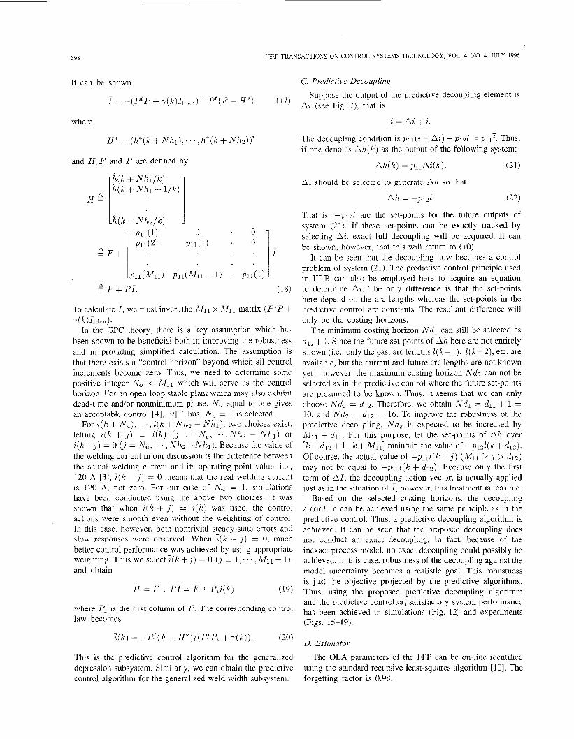
Fig. 9. Simulated predictive control with slight weighting -(h = 0.002, Y b = 0 and smoothing factor cy = 0.9. When ~h = 0 was used, the system was not stable. When the slight control weight 7 h = 0.002 is used, the system becomes stable.

Because only two two-parameter recursive least-squares calculations are performed, the computation for the on-line identification is negligible in comparison with the image processing and predictive algorithms. The time needed for the adaptive control computation, including the predictive control algorithms and on-line identification, is less than 150 ms. Thus, the sampling interval of 0.5 second can be guaranteed.

IV. SIMULATION

Two types of simulations will be done. In the first type of simulation, the welding process is simulated using the nominal model. Also, the nominal model will be used as the a priori model. This type of simulation is used to determine the default parameters in the control and decoupling algorithms, i.e., the weights and smoothing factors. In the second type of simulation, the robustness of the designed controller will be tested using different typical welding conditions. Six individual models acquired under six typical welding conditions [3] will be used to simulate the process. The nominal model will be used as the a priori model. If the system works well under different typical conditions, then the designed control system will be robust in the practice of welding.

For simplicity, the weights and smoothing factors in the control and decoupling are selected to be the same. The simulation time is 200 sampling intervals as in the experiments.

Denote the weights of the control actions in the generalized depression and generalized width subsystems as Y h and Yb,

respectively. It is observed that oscillation may be generated if Y b = 0 and Y h = 0 are used. When T h = 0.002 and ~b = 0 are used, the oscillation is eliminated (Fig. 9). The control actions, however, still frequently fluctuate in the initial regulation period (Fig. 9). This control action fluctuation is not desirable in a practical control system. When greater weights are used, the current tends to be smoother. The regulation speed is decreased, however, and larger steady-state errors are observed. In the initial regulation period, large and frequent fluctuations are possible because the large error in the initial regulation period may drive the controller to yield energetic actions. To restrict the control actions, a larger weight can be used. After the initial regulation period, however, the errors between the actual and desired outputs become smaller. Smaller errors tend to suppress the control actions. In this case, if a larger weight is used, the control actions will become

-0.01 0 20 40 60 80 100

time (second) (a)

so 45

(D E 30 0 m 25 g 0 20 0 x 15 x -10 W Q 5 “ E : o

h &

0 10 20 30 40 50 60 70 80 90 100 time (second)

(b)

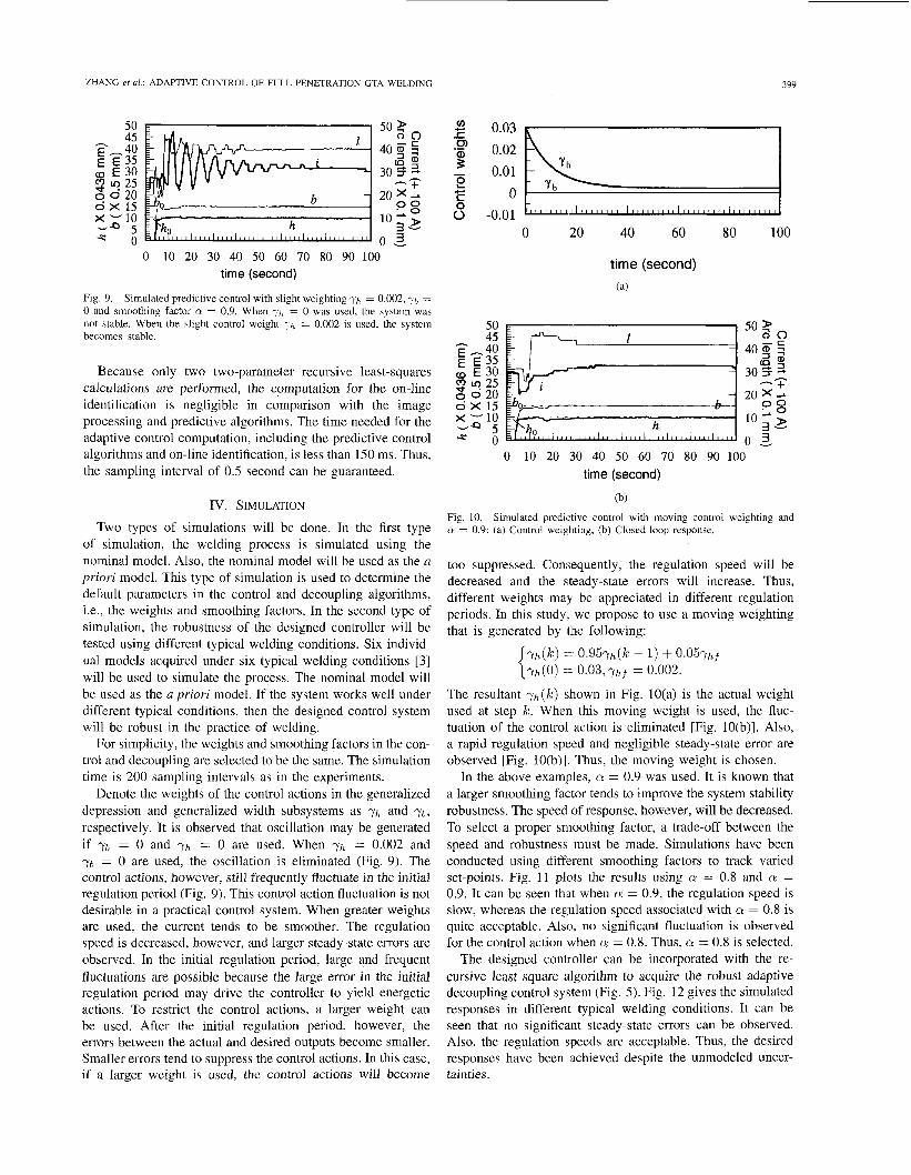
Fig. 10. cy = 0.9: (a) Control weighting, (b) Closed-loop response.

Simulated predictive control with moving control weighting and

too suppressed. Consequently, the regulation speed will be decreased and the steady-state errors will increase. Thus, different weights may be appreciated in different regulation periods. In this study, we propose to use a moving weighting that is generated by the following:

The resultant ~ h ( k ) shown in Fig. 10(a) is the actual weight used at step I C . When this moving weight is used, the fluctuation of the control action is eliminated [Fig. 10(b)]. Also, a rapid regulation speed and negligible steady-state error are observed [Fig. 10(b)]. Thus, the moving weight is chosen.

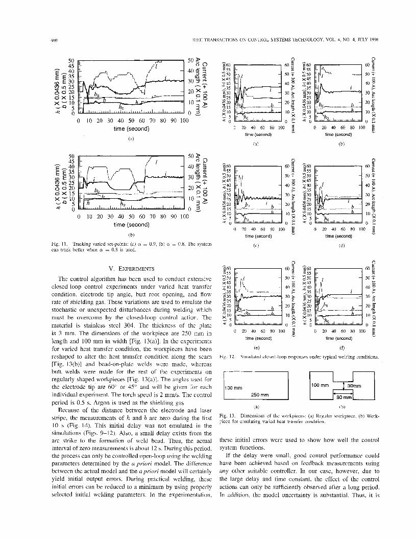
In the above examples, a = 0.9 was used. It is known that a larger smoothing factor tends to improve the system stability robustness. The speed of response, however, will be decreased. To select a proper smoothing factor, a trade-off between the speed and robustness must be made. Simulations have been conducted using different smoothing factors to track varied set-points. Fig. 11 plots the results using a = 0.8 and a = 0.9. It can be seen that when Q = 0.9, the regulation speed is slow, whereas the regulation speed associated with a = 0.8 is quite acceptable. Also, no significant fluctuation is observed for the control action when a = 0.8. Thus, a = 0.8 is selected.

The designed controller can be incorporated with the recursive least square algorithm to acquire the robust adaptive decoupling control system (Fig. 5) . Fig. 12 gives the simulated responses in different typical welding conditions. It can be seen that no significant steady-state errors can be observed. Also, the regulation speeds are acceptable. Thus, the desired responses have been achieved despite the unmodeled uncertainties.


50 45

E -40 E E 3 5 a E 30 m 25

0 0 20 o X 15

-

x-10 v9 5 C O

X’lO up 5 a 0

0 10 20 30 40 50 60 70 80 90 100 time (second)

(a)

- + 20 x - P g 10 - 9 3-

O w 3

30 5z

10 - ; - +

20 x - P O

3 - o w 3 0 10 20 30 40 50 60 70 80 90 100

time (second)

(b)

Fig. 11. can track better when cy = 0.8 is used.

Tracking varied set-points: (a) cy = 0.9, (b) a = 0.8. The system

V. EXPERIMENTS

The control algorithm has been used to conduct extensive closed-loop control experiments under varied heat transfer condition, electrode tip angle, butt root opening, and flow rate of shielding gas. These variations are used to emulate the stochastic or unexpected disturbances during welding which must be overcome by the closed-loop control action. The material is stainless steel 304. The thickness of the plate is 3 mm. The dimensions of the workpiece are 250 mm in length and 100 mm in width [Fig. 13(a)]. In the experiments for varied heat transfer condition, the workpieces have been reshaped to alter the heat transfer condition along the seam [Fig. 13(b)] and bead-on-plate welds were made, whereas butt welds were made for the rest of the experiments on regularly shaped workpieces [Fig. 13(a)]. The angles used for the electrode tip are 60” or 45” and will be given for each individual experiment. The torch speed is 2 m d s . The control period is 0.5 s. Argon is used as the shielding gas.

Because of the distance between the electrode and laser stripe, the measurements of h and b are zero during the first 10 s (Fig. 14). This initial delay was not emulated in the simulations (Figs. 9-12). Also, a small delay exists from the arc strike to the formation of weld bead. Thus, the actual interval of zero measurements is about 12 s. During this period, the process can only be controlled open-loop using the welding parameters determined by the a priori model. The difference between the actual model and the a priori model will certainly yield initial output errors. During practical welding, these initial errors can be reduced to a minimum by using properly selected initial welding parameters. In the experimentation,

-60 2 55 2 50 x 45 g 40 2 3 5 5 30

- 5 ‘ 0

h

E 60 55

0 50 x 45 24 2 3 5

8 15

‘c!

8 30 25 20

g 10 - 5 = 0

2 50 x 45 g 40 ,35

z 20

8 30 25

8 15

- 5 : 10

= 0

20 $ E+ 10 h

X

0 : 0 20 40 60 80 100

time (second) v

(a)

n . _ 60 $ r 50 3

40 f -

30 ; 20 $

6. 10 h

X o s 0 20 40 60 80 100 E

v

time (second)

(b)

50 C

20

10 ti X o s

60 - 50 3

40 E v

30 5 20 $ E 10 h

X o e 0 20 40 60 80 100 E 0 20 40 60 80 100 E

v v time (second) time (second)

(c) (dl

h

50 3

40 F 30

20 E

o e 09 E

10 h X

-60 55

2 50 x 45

40 2 3 5

g 10 - 5 ‘ 0

50 3

40

30

20 E 10 Q . . o e

0 20 40 60 80 100 E 0 20 40 60 80 100 time (second) time (second)

v v

(e) (0 Fig. 12. Simulated closed-loop responses under typical welding conditions.

I I

100 mm

(a) (b)

Fig. 13. piece for emulating varied heat transfer condition.

Dimensions of the workpieces: (a) Regular workpiece, (b) Work-

these initial errors were used to show how well the control system functions.

If the delay were small, good control performance could have been achieved based on feedback measurements using any other suitable controller. In our case, however, due to the large delay and time constant, the effect of the control actions can only be sufficiently observed after a long period. In addition, the model uncertainty is substantial. Thus, it is

ZHANG er al.: ADAPTIVE CONTROL OF FULL PENETRATION GTA WELDING 401

...

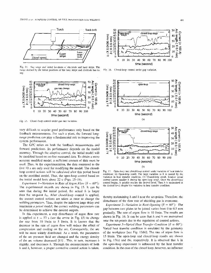
stripe / - Travel meed V

Fig. 14. Sag range and initial locations of electrode and laser stripe. The range defined by the initial positions of the laser stripe and electrode has no sag.

closed-loop range .M gas rate, change 40%: .-

o >

0 10 20 30 40 50 60 70 80 90 100 time (second)

Fig. 15. Closed-loop control under gas rate variation.

very difficult to acquire good performance only based on the feedback measurements. For such a plant, the forward long- range prediction can play a fundamental role in improving the system performance.

The GPC relies on both the feedback measurements and forward predictions. Its performance depends on the model accuracy. Through the adaptive control, the initial model will be modified based on on-line measured data. To obtain a more accurate modified model, a sufficient amount of data must be used. Thus, in the experimentation, the data measured in the first 10 s are only used for modifying the model. The closed- loop control actions will be calculated after this period based on the modified model. Thus, the open-loop control based on the initial model lasts about 22 s (Figs. 15-19).

Experiment I-Variation in Rate of Argon Flow (6' = 60"): The experimental records are shown in Fig. 15. It can be seen that during the initial period, the actual h is larger than the set-point ho. After closed-loop control is applied, the correct control actions are taken at once to change the welding parameters. Thus, despite the inherent large delay and inaccurate a priori model, the correct welding parameters can be determined to achieve the desired outputs.

In this experiment, a step disturbance of argon flow rate is applied at t = 53 s (see the arrow in Fig. 15) to change the rate from 10 l/min to 5 l/min. It is known that the decrease in the rate of argon flow will reduce the effect of compression and cooling on the arc. Consequently, the arc will be more widely distributed. As a result, the parameters of the arc pressure field are changed and the energy density of the arc volume decreased [ l l ] . This, in turn, increases b slightly, and decreases h. Through the measurements of both h and b, however, a proper corrective control action is taken,

50 45

E -40 E E35 UJ E30

U? 25 x 0 20 0 x 15

h

x -10 UQ 5 C O

0 10 20 30 40 50 60 70 80 90 100 time (second)

Fig. 16. Closed-loop control under gap variation

50 45

E -40 E E 3 5

E 30 0 UI 25 x 0 20 0 x 15

h

~~

x -10 5 * o

50 45

h

LD 25 x 0 20 0 x 15 x -10

5 - = o

50 2 0 0

40 5 5 30 3 2

--3 20 x -

3 8 3 2

0 , 3 0 10 20 30 40 50 60 70 80 90 100

time (second)

(a)

closed-loop range

0 10 20 30 40 50 60 70 80 90 100 time (second)

(b)

Fig. 17. Open-loop and closed-loop control under variation of heat transfer condition: (a) Open-loop result. The large variation in h is caused by the variation in heat transfer condition, (b) Closed-loop result. Smaller initial current causes smaller h during the open-loop range. Once the closed-loop control begins, h quickly reaches the desired level. Then h is maintained at the desired level despite the variation in heat transfer condition.

thereby maintaining h, and b near the set-points. Therefore, the disturbance of the flow rate of shielding gas is overcome.

Experiment 2-Variation in Root Opening (6' = 60"): The gap between two plates to be joined varies from 0 to 0.5 mm gradually. The rate of argon flow is 10 l/min. The results are shown in Fig. 16. It can be seen that h and b are maintained near the set-points due to the regulation of control actions.

Experiment 3-Varied Heat Transfer Condition (6' = 60"): Varied heat transfer condition is emulated by the geometry of the workpiece [see Fig. 13(b)]. The rate of argon flow is 15 l/min. The open-loop and closed-loop results are shown in Fig. 17(a) and (b), respectively. It is observed that h in the open-loop experiment is influenced by the heat transfer condition. In the case of the closed loop, however, no influence

402 IEEE TW LNSACTIONS ON CONTROL SYSTEMS TECHNOLOGY, VOL. 4, NO. 4, JULY 1996

50 45

h

2;: (o E 30 0 10 25 B 0 20 o X 15 x -10 UcI 5 C O

open-loop 3 0 10 20 30 40 50 60 70 80 90 100

time (second)

(a)

45 50 50 $ 2

x -10 10 ,% 40 5 7

30 F z (o E 30 0 m 25 - + B 0 20 20 x - o X 15 00

uQ 5 C O 0 2

h

caz z::

0 10 20 30 40 50 60 70 80 90 100 time (second)

(b)

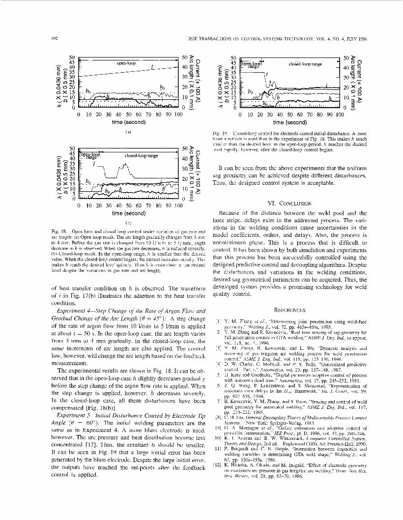
Fig. 18. Open-loop and closed-loop control under variation of gas rate and arc length: (a) Open-loop result. The arc length gradually changes from 3 mm to 4 mm. Before the gas rate is changed from 10 I / min to 5 / / m i n . slight decrease in h is observed. When the gas rate decreases, h is reduced severely, (b) Closed-loop result. In the open-loop range, h is smaller than the desired value. When the closed-loop control begins, the current increases rapidly. This makes h reach the desired level quickly. Then h is maintained at the desired level despite the variations in gas rate and arc length.

of heat transfer condition on h is observed. The waveform of i in Fig. 17(b) illustrates the adaption to the heat transfer condition.

Experiment 4-Step Change of the Rate of Argon Flow and Gradual Change of the Arc Length (6’ = 45’): A step change of the rate of argon flow from 10 Umin to 5 l/min is applied at about t = 50 s. In the open-loop case, the arc length varies from 3 mm to 4 mm gradually. In the closed-loop case, the same increments of arc length are also applied. The control law, however, will change the arc length based on the feedback measurements.

The experimental results are shown in Fig. 18. It can be observed that in the open-loop case h slightly decreases gradually before the step change of the argon flow rate is applied. When the step change is applied, however, h decreases severely. In the closed-loop case, all these disturbances have been compensated [Fig. 18(b)].

Experiment 5-Initial Disturbance Caused by Electrode Tip Angle (6‘ = 60”): The initial welding parameters are the same as in Experiment 4. A more blunt electrode is used, however. The arc pressure and heat distribution become less concentrated [12]. Thus, the resultant h should be smaller. It can be seen in Fig. 19 that a large initial error has been generated by the blunt electrode. Despite the large initial error, the outputs have reached the set-points after the feedback control is applied.

x -10 5 J : o

. closed-loop range -

0 10 20 30 40 50 60 70 80 90 100 time (second)

Fig. 19. Closed-loop control for electrode caused initial disturbance. A more blunt electrode is used than in the experiment of Fig. 18. This makes h much smaller than the desired level in the open-loop period. h reaches the desired level rapidly, however, after the closed-loop control begins.

It can be seen from the above experiments that the uniform sag geometry can be achieved despite different disturbances. Thus, the designed control system is acceptable.

VI. CONCLUSION

Because of the distance between the weld pool and the laser stripe, delays exist in the addressed process. The variations in the welding conditions cause uncertainties in the model coefficients, orders, and delays. Also, the process is nonminimum phase. This is a process that is difficult to control. It has been shown by both simulation and experiments that this process has been successfully controlled using the designed predictive control and decoupling algorithms. Despite the disturbances and variations in the welding conditions, desired sag geometrical parameters can be acquired. Thus, the developed system provides a promising technology for weld quality control.

REFERENCES

[l] Y . M. Zhang et al., “Determining joint penetration using weld-face geometry,” Welding J., vol. 72, pp. 463s469s, 1993.

[2] Y . M. Zhang and R. Kovacevic, “Real-time sensing of sag geometry for full penetration control in GTA welding,” ASME J. Eng. Znd., to appear, vol. 118, no. 4, 1996.

[ 3 ] Y . M. Zhang, R. Kovacevic, and L. Wu, “Dynamic analysis and modeling of gas tungsten arc welding process for weld penetration control,” ASME J. Eng. Ind., vol. 118, pp. 123-136, 1996.

[4] D. W. Clarke, C. Mohtadi, and P. S. Tuffs, “Generalized predictive control-Part 1,” Automatica, vol. 23, pp. 137-148, 1987.

[5] H. Kurz and Goedecke, “Digital parameter-adaptive control of process with unknown dead time,” Automatica, vol. 17, pp. 245-252, 1981.

[6] 2. Q. Wang, P. Lundestrom, and S. Skogestad, “Representation of uncertain time delays in the H , framework,” Int. J. Contr., vol. 59, pp. 627-638, 1994.

[7] R. Kovacevic, Y. M. Zhang, and S. Ruan, “Sensing and control of weld pool geometry for automated welding,” ASME J. Eng. Ind., vol. 117, pp. 210-222, 1995.

[8] C. H. Liu, General Decoupling Theory of Multivariable Process Control Systems. New York: Springer-Verlag, 1983.

[9] G. A. Montague et al., “Online estimation and adaptive control of penicillin fermentation,” IEE Proc., pt. D, 1986, vol. 33, pp. 240-246.

[ lo] K. J. Astrom and B. W. Wittenmark, Computer Controlled System: Theory and Design, 2nd ed. Englewood Cliffs, NJ: Prentice-Hall, 1990.

[11] P. Burgardt and C. R. Heiple, “Interaction between impurities and welding variables in determining GTA weld shape,” Welding J. , vol.

1121 K. Hiraoka, A. Okada, and M. Inagaki, “Effect of electrode geometry on maximum arc pressure in gas tungsten arc welding,” Trans. Nut. Res. Inst. Metals, vol. 28, pp. 63-70, 1986.

67, pp. 150~-155~, 1986.


Yu M. Zhang received the B.S. and M.S. degrees in control engineering, and the Ph.D. degree in mechanical engineering, all from Harbin Institute of Technology (HIT), Harbin, China, in 1982, 1984, and 1990, respectively.

He joined the National Key Laboratory for Ad- vanced Welding Production Technology at HIT in 1984 as a Junior Lecturer, and was promoted to Professor in 1993. Since 1991, he has been with the Center for Robotics and Manufacturing Systems at the Iiniversitv of Kentuckv. Lexington. Kentuckv.

I,in Li was born in Shengmu, Shaanxi, China, on January 7, 1964. He received the B.S degree in nwchanical engineering from Xian Jiaotong Univer- sity, Xian, China, in 1984, and the M.S degree in mechanical engineering from the Harhin Institute of Technology, Harbin, China, in 1990. He is currently a Ph.D. candidate in mechanical engineering at the Iiniversity of Kentucky, Lexington

He was a Welding Engineer at Harbin Boiler Works, Harbin, China, during 1984-1987, and a Software Engineer in the comuuter center of the

2 , U I .I, ~~~ ~~~~ ~~~~ L

as Research Fellow and has helped Prof. R. Kovacevic develop an active welding and industrial application program. His book, Modern Control of Welding Process-Analysis and Design (Harbin, China: HIT Press, 1990) is an assigned graduate textbook at HIT. He holds one U.S. patent and is the author or co-author of 40 journal papers. His research interests include dynamic modeling, control, machine vision, and industrial applications.

People’s Bank of China, from 1990 to 1994. In 1994-1995, he was with the Center for Robotics and Manufacturing Systems at the University of Kentucky as a Researcher. His research interests include welding processes, control, machine vision, and industrial applications.

Radovan Kovacevic received the B S and M S degrees in mechanical engineering from the Uni- versity of Belgrade, Yugoslavia, in 1969 and 1972, respectively, and the Ph D degree in mechanical engineering from the Univer\ity of Montenegro, Podgorica, Yugoslavia, in 1978

He joined the faculty of the Department of Me- chanical Engineering at the University of Kentucky, Lexington, in January 1991 and was promoted to Full Professor in May of 1995 He is an Hon- orary Consultant Professor at the Harbin Institute of

Technology, Harbin, China. He was an Associate Professor of Mechanical Engineering dt Syrdcuye University, Syracuse, NY (1987-1990), and, for more than 16 years, was a faculty member at the University of Montenegro, Podgorica, Yugoslavia. He 15 the Director of the Laboratory for Advanced Manufacturing Processes, Welding Research and Development Laboratory, dnd Machine Vision and Neural Networks Laboratory at the Center for Robotics and Manufacturing Systems His research includes phyws of tradi- tional and advanced manufacturing processe?, modeling, on-line monitoring, and control of manufacturing processes and welding processes, and machine vision in quality control He ha5 published more than 180 technical papers, four hooks, and holds two U.S patents

394 adaptive control full penetration gas tungsten …ymzhang/papers/ieee control systems...394 ieee...

Documents