38747320 ullmann s enc of industrial chemistry polimerization
TRANSCRIPT

c© 2005 Wiley-VCH Verlag GmbH & Co. KGaA, Weinheim10.1002/14356007.a21 305
Polymerization Processes 1
Polymerization Processes
Archie E. Hamielec, Institute for Polymer Production Technology, Department of Chemical Engineering,
McMaster University, Hamilton, Ontario, L8S 4L7, Canada
Hidetaka Tobita, Department of Materials Science and Engineering, Fukui University, Fukui, 910, Japan
1. Introduction–Trends in Poly-
mer Reaction Engineering . . . 7
2. Polymerization Mechanisms
and Kinetics . . . . . . . . . . . . . 8
2.1. Step-Growth Polymerization . . 9
2.1.1. Linear Polymerization . . . . . . . 9
2.1.2. Interfacial Polymerization . . . . . 12
2.1.3. Nonlinear Polymerization . . . . . 12
2.2. Chain-Growth Polymerization . 14
2.2.1. Free-Radical Polymerization . . . 15
2.2.1.1. Initiation . . . . . . . . . . . . . . . 16
2.2.1.2. Propagation . . . . . . . . . . . . . . 18
2.2.1.3. Termination . . . . . . . . . . . . . 19
2.2.1.4. Chain Transfer to Small
Molecules . . . . . . . . . . . . . . . 21
2.2.1.5. Kinetics of Linear Polymerization 22
2.2.1.6. Effect of Temperature . . . . . . . 25
2.2.1.7. Branching Reactions . . . . . . . . 26
2.2.2. Ionic Polymerization . . . . . . . . 28
2.2.2.1. Cationic Polymerization . . . . . . 29
2.2.2.2. Anionic Polymerization . . . . . . 30
2.2.2.3. Ziegler – Natta Polymerization . . 32
2.3. Copolymerization . . . . . . . . . 34
2.3.1. Copolymer Composition . . . . . 35
2.3.2. Kinetics of Copolymerization . . 37
2.3.3. Copolymerization of Vinyl and
Divinyl Monomers . . . . . . . . . 38
3. Polymerization Processes and
Reactor Modeling . . . . . . . . . 40
3.1. Introduction . . . . . . . . . . . . . 40
3.2. Processes and Reactor Modeling
for Step-Growth Polymerization 41
3.2.1. Types of Reactors and Reactor
Modeling . . . . . . . . . . . . . . . 41
3.2.2. Specific Processes . . . . . . . . . 44
3.3. Processes and Reactor Modeling
for Chain-Growth Polymeriza-
tion . . . . . . . . . . . . . . . . . . . 47
3.3.1. Material Balance Equations for
Batch, Semi-Batch, and Continu-
ous Reactors . . . . . . . . . . . . . 47
3.3.1.1. Rates of Reaction and Copolymer
Composition . . . . . . . . . . . . . 48
3.3.1.2. Molecular Masses, Long-Chain
Branching, and Cross-Linking . . 50
3.3.2. Examples of Free-Radical Poly-
merization . . . . . . . . . . . . . . 50
3.3.2.1. Homopolymerization – Linear
Chains . . . . . . . . . . . . . . . . . 50
3.3.2.2. Copolymerization – Linear
Chains . . . . . . . . . . . . . . . . . 54
3.3.2.3. Copolymerization – Long-Chain
Branching . . . . . . . . . . . . . . . 55
3.3.3. Polymerization Processes . . . . . 55
3.3.3.1. Solution Polymerization . . . . . . 55
3.3.3.1.1. Polymer Soluble in Monomer . . 55
3.3.3.1.2. Addition of a Solvent in which
both Monomer and Polymer are
Miscible . . . . . . . . . . . . . . . . 55
3.3.3.1.3. Polymer – Polymer Demixing dur-
ing Polymerization . . . . . . . . . 56
3.3.3.2. Precipitation Polymerization . . . 57
3.3.3.2.1. Polymer Insoluble in its Monomer 57
3.3.3.2.2. Monomer Functioning as Solvent
for the Polymer . . . . . . . . . . . 60
3.3.3.3. Suspension Polymerization . . . . 63
3.3.3.3.1. Qualitative Description . . . . . . 64
3.3.3.3.2. Dispersants . . . . . . . . . . . . . . 66
3.3.3.3.3. Mechanism of Particle Formation 67
3.3.3.3.4. Industrial Applications . . . . . . . 70
3.3.3.4. Emulsion Polymerization . . . . . 73
3.3.3.4.1. Theories of Emulsion Polymeriza-
tion . . . . . . . . . . . . . . . . . . . 74
3.3.3.4.2. Physicochemical Parameters of
Dispersions . . . . . . . . . . . . . . 85
3.3.3.4.3. Inverse Emulsion Polymerization 88
3.3.3.4.4. Semi-Batch Emulsion Polymeri-
zation . . . . . . . . . . . . . . . . . 89
3.3.3.4.5. Continuous Emulsion Polymeri-
zation . . . . . . . . . . . . . . . . . 90
3.3.4. Miscellaneous Processes . . . . . 93
3.3.5. Ionic Polymerization Modeling . 96
3.3.5.1. Introduction . . . . . . . . . . . . . 96
3.3.5.2. Heterogeneous Coordination Po-
lymerization . . . . . . . . . . . . . 96
2 Polymerization Processes
3.3.6. Process Variables, Reactor Dy-
namics/ Stability, On-Line Moni-
toring and Control . . . . . . . . . 97
3.3.6.1. Influence of Reactor Type and
Configuration on Molecular Mass
and Copolymer Composition Dis-
tributions, and on Long-Chain
Branching and Cross-Linking . . 97
3.3.6.1.1. Monomer Coupling with Bimo-
lecular Termination Plug Flow and
Batch Reactors (CPFR/BR) . . . . 99
3.3.6.1.2. Monomer Coupling Without Ter-
mination Plug Flow and Batch Re-
actors (CPFR/BR) . . . . . . . . . 103
3.3.6.1.3. Polymer Coupling . . . . . . . . . 104
3.3.6.1.4. Copolymerization . . . . . . . . . . 107
3.3.6.1.5. Long-Chain Branching and Cross-
Linking . . . . . . . . . . . . . . . . 109
3.3.6.2. Reactor Dynamics and Stability . 111
3.3.6.3. On-Line Monitoring and Control 112
4. References . . . . . . . . . . . . . . 114
Sections 3.3.3.1 – 3.3.3.5 and 3.3.6.1 werebased on the article Polymerisationstechnik inUllmann’s, 4th ed. written by Heinz Gerrens.
List of symbols
A chemical species; vacant adsorption site[A] concentration of species A[A]0 initial concentration of species AA1, A2, A3 adjustable parametersABS acrylonitrile – butadiene – styrene
rubber-modified copolymerACA aminocaproic acidA (h) energy required to separate to a distance
h=∞, two drops of diameter d=1 ini-tially separated by a distance h0
Am surface area of micellesAp surface area of polymer particlesB chemical speciesBHET bis-hydroxyethyl terephthalateBR batch reactorCpi dimensionless moments of polymer dis-
tribution for chain transfer to polymer[= K fp Qi/(Kp[M])]
CS surfactant concentrationCCD chemical composition distributionCMC critical micelle concentrationCPFR continuous plug flow reactorCSTR continuous stirred-tank reactor with an
ideal residence-time distributionCTA chain-transfer agentd particle diameterd average particle diameterd32 Sauter mean diameter of a spherical-
particle suspensiond50 diameter at which 50 wt % of particles
pass through a sievedmin minimum particle diameterdmax maximum particle diameter
D stirrer diameterDop mean diffusion coefficient for
oligomeric radicals and latex particlesDMT dimethyl terephthalateEd activation energy for initiator decompo-
sitionE/E0 mass fraction of material passing out of
reactor with a residence time t to t + dt
Ef activation energy for chain-transfer re-action
EL activation energy for average chainlengths
EN activation energy for polymer particlenucleation
Ep activation energy for propagationER activation energy for polymerizationE (t) residence-time distribution for a flow
reactor at steady stateEt activation energy for bimolecular termi-
nationEu modified power numberEG ethylene glycolEGDMA ethylene glycol dimethacrylateEPS expandable polystyreneESR electron spin resonance spectroscopyf initiator efficiency; functionality of
monomerfj mole fraction of monomer of type j
Fi, in molar flow rate of monomer of type i
into the reactorFin total molar flow rate (of all monomer
types) into the reactorFIi, in molar flow rate of initiator of type i into
the reactorFj mole fraction of monomer of type j,
chemically bound in polymer producedinstantaneously
Polymerization Processes 3
Fj mole fraction of monomer of type j
chemically bound in accumulated poly-mer
F1 mole fraction of monomer 1 (containingan abstractable atom) in accumulatedpolymer
F2 mole fraction of monomer 2 (containinga reactive carbon – carbon bond
Fpi, in molar flow rate of monomer of type i
chemically bound in polymer into thereactor
Fr Froude numberFT, in molar flow rate of chain-transfer agent
T into the reactorG+ counterionGPC gel permeation chromatographyHCSTR homogeneous CSTRHDPE high-density polyethyleneH – H Hui – Hamielec styrene polymerization
modelHIPS high-impact polystyreneI initiator or catalyst[I] concentration of initiator or catalystK chemical rate constant; equilibrium
constantKa absorption constant for oligomeric rad-
icals entering polymer particlesKA adsorption rate constantKd initiator decomposition constantKdp depropagation constantKD desorption rate constantK f j
irate constant for polymeric radical
of type i abstracting an atom frommonomer of type j chemically boundin polymer
K fm transfer to monomer rate constantK fp rate constant for chain transfer to poly-
merK fT rate constant for chain transfer to CTAK fTi rate constant for chain transfer from
polymeric radical of type i to CTAK fX transfer to small molecule X rate con-
stantK i rate constant for monomer adding to a
primary radicalKp propagation rate constantK ′p propagation rate constant for transfer
radicalK−p propagation rate constant for free ion
K±p propagation rate constant for ion pair
Kp∗ rate constant for polymeric radicalsadding to pendant double bonds onpolymer chains
Kpji, Kij propagation rate constant for
monomer of type j adding to polymericactive center of type i
Kpij rate constant for polymeric radical oftype i adding to a double bond ona monomer unit of type j chemicallybound in the polymer
Kpijkpropagation rate constant for monomerof type k adding to a polymeric activecenter of type ij
Kt total bimolecular termination constant(Ktc + Ktd)
Kt0 total bimolecular termination constantat zero conversion of monomer
Ktc rate constant for bimolecular termina-tion by combination
Ktcijtermination by combination rate con-stant for polymeric radicals of types i
and j (chemical control)KtcN number-average bimolecular termina-
tion constant by combinationKtd rate constant for bimolecular termina-
tion by disproportionationKtdij
termination by disproportionation rateconstant for polymeric radicals of typesi and j (chemical control)
KtdN number-average bimolecular termina-tion constant by disproportionation
KtN total number-average bimolecular ter-mination constant
Ktp termination rate constant in polymerparticles
Kt (r, s) total bivariate distribution fordiffusion-controlled bimolecular ter-mination of polymeric species of chainlengths r and s
Ktw termination rate constant in aqueousphase
KtW, KtZ total weight- and z-average bimolec-ular termination constants
L characteristic length of energy-con-taining large eddies
L length of path traversed by a growingradical from its point of origin to thepoint where it precipitates
L reactor lengthLALLS low-angle laser light scatteringLCB long-chain branching

4 Polymerization Processes
LDPE low-density polyethyleneLLDPE linear low-density polyethylenemi number of moles of monomer i in ter-
polymer (Eq. 3.101)Mc average molecular mass between cross-
linksMi monomer of type i
Mm aggregation number for emulsifiermolecules in micelles
Mmi molecular mass of monomer of type i
MN, MW, MZ , MZ+1 number-, weight-, Z andZ + 1-average molar mass (molecularmass, respectively)
[M] total monomer concentration[M]0 initial monomer concentration;
monomer concentration in feed[M]c equilibrium concentration of monomer
at the ceiling temperature[Mi] concentration of monomer of type i
[M]p concentration of monomer in the poly-mer particles
M – H Marten – Hamielec polymerizationmodel
MMA methyl methacrylateMWD molecular mass distribution (molar
mass distribution)n number of monomer typesn order of reactionn average number of radicals per particleN0, N number of functional groups at time
zero and t
N total number of moles in the reactor;stirrer speed
NA number of moles of A-functionalgroups; Avogadro number
NA0initial number of moles of A-functionalgroups
NB number of moles of B-functionalgroups
NB0initial number of moles of B-functionalgroups
Ni moles of monomer of type i in the reac-tor
N I number of moles of initiator in the re-actor; number of growing chains
N I0 initial number of moles of initiator inthe reactor
N Ii moles of initiator of type i in the reactorN (r) number chain length distribution
(number-fraction of polymer moleculesof chain length r)
NM number of monomer units; numberof micelles; number of monomermolecules consumed
Nn number of polymer particles containingn radicals
Np number of polymer particles per unitvolume
NT moles of CTA in reactorNBR nitrile – butadiene rubberNIRS near infrared spectroscopyp conversion of functional groupspc critical thresholdP growing polymer particle; polymerPc conversion of functional groups at gela-
tion pointPcr critical chain length for precipitationPi moles of monomer of type i chemically
bound in polymer in the reactorPij polymer containing i units of monomer
of type 1 and j units of monomer of type2
[Pm] concentration of polymer with chainlength m
Pm,n dead polymer chain containing m unitsof monomer 1 and n units of monomer2
PN number-average chain length of poly-mer produced instantaneously
PN number-average chain length of accu-mulated polymer
PsolN number-average chain length of sol
moleculesPr polymer molecule of chain length r
PW weight-average chain length of polymerproduced instantaneously
PW weight-average chain length of accu-mulated polymer
PsolW weight-average chain length of sol
moleculesPDI polydispersity index of polymer pro-
duced instantaneouslyPDI polydispersity index of accumulated
polymerPE polyethylenePEK polyetherketonePES polyethersulfonePETP poly(ethylene terephthalate)PFR plug-flow reactorPMMA poly(methyl methacrylate)PP polypropylenePPS poly(phenylene sulfide)PS polystyrene
Polymerization Processes 5
PSD particle size distributionPVAL poly(vinyl alcohol), partially hydro-
lyzedPVC poly(vinyl chloride)P∗ polymeric active center[P∗] concentration of polymeric active cen-
ters (ionic or radical type)P∗i polymeric active center with active cen-
ter located on monomer of type i chem-ically bound in the polymer chain
P∗ij polymeric active center with active cen-ter located on monomer of type j whichis adjacent to monomer of type i chem-ically bound in the polymer chain
P∗m,n,i polymer chain containing m units ofmonomer 1, n units of monomer 2, withactive center on monomer i
Qi i-th moment of the dead polymer distri-bution
r polymer chain lengthr polymer particle radiusrM micelle radiusrp polymer particle radiusr1, r2 reactivity ratiosR gas constant
R•
polymeric radical
[R•
] concentration of polymeric radicalsRe Reynolds numberRf rate of chain transferRFP (r) production rate of polymer molecules
with chain length r
Ri rate of radical entry into polymer parti-cles
R∗in initiator/catalyst fragment with an ac-tive center
R•
in initiator radical with a peroxide endgroup
R•
in initiator or primary radical
[R•
in] concentration of primary radicalsRi,w radical generation rate in the aqueous
phase via initiator decompositionRI rate of initiation (rate of generation of
polymeric radicals with chain lengthunity via initiation)
RIM reaction injection moldingRp rate of polymerization (monomer con-
sumption rate via propagation reac-tions)
Rpiconsumption rate of monomer of type i
via propagation reactions
Rpij consumption rate of monomer of type j
by propagation with polymeric radicalsof type i
Rp,o initial polymerization rate
R•
r polymeric radical of chain length r
[R•
r ] concentration of polymeric radicals ofchain length r
Rt rate of bimolecular terminationRtc rate of bimolecular termination by com-
binationRtd rate of bimolecular termination by dis-
proportionationRTD residence time distribution[R•
]w concentration of radicals in the aqueousphase
∆S0 entropy change of polymerization at thestandard state
S surface area of polymer particleS surfactantSAN styrene – acrylonitrile copolymerSBR styrene – butadiene rubberSCSTR segregated CSTRSSH stationary-state hypothesist timet1/2 half-life of initiatort1 polymer particle nucleation timets time when polymer particle nucleation
ceasesT temperatureT chain-transfer agent
T•
CTA transfer radicalT c ceiling temperatureTg glass transition temperatureTPA terephthalic acidTREF temperature rise elution fractionationU MWD nonuniformity indexv volume of polymer particlev volumetric flow rate into and out of re-
actorvc capture rate of radicals by polymer par-
ticlesvf flocculation rate of precipitated (pri-
mary) polymer particlesV volume of reacting mixture in the reac-
torV0 intial volume of reacting mixture in the
reactorV in total volumetric flow rate into the reac-
torVout total volumetric flow rate out of the re-
actor

6 Polymerization Processes
Vm specific volume of monomerVp specific volume of polymerV s volume of solvent in the reactorV s, in volumetric flow rate of solvent into the
reactorVCM vinyl chloride monomerW e Weber numberWg weight fraction of gelW (r) weight chain length distribution
(weight fraction of polymer of chainlength r)
W (r), W (r, t) “instantaneous” weight chainlength distribution
W (r), W (r, t) weight chain length distributionof accumulated polymer
W1, W2 weight fractions of homopolymers 1and 2
x monomer conversionX small molecule with a labile atomX•
transfer radicalz exponent indicating dependence of Np
on emulsifier and initiator concentra-tions
α stoichiometric imbalance∆α1, ∆α2 differences between thermal expan-
sion coefficients above and below Tg
for homopolymers 1 and 2β kinetic parameter (dimensionless)γ kinetic parameter (dimensionless)∗γprec volume fraction of precipitantδ kinetic parameter (dimensionless)ε characterizes the radical capture effi-
ciency of latex particles relative to mi-celles; energy-dissipation rate
ε mean rate of energy dissipation per unitmass
η moles of monomer consumed per activesite (≡ PN)
ηc viscosity of continuous phaseηd viscosity of disperse phasec density of continuous phased density of disperse phaseel elastic cross-link densitymi
density of monomer i
p density of polymerσ standard deviationσ2 statistical varianceσ interfacial tensionσSG interfacial tension between solid and
gasσSM interfacial tension between solid and
monomer
σSW interfacial tension between solid andwater
σWG interfacial tension between water andgas
σWM interfacial tension between water andmonomer
τ kinetic parameter (dimensionless)τ mean residence timeϕ phase volume ratioϕ, ϕ′ probability of propagationϕm volume fraction of monomerϕp volume fraction of polymer
ϕ•
i number fraction of polymeric radicalsof type i (terminal model)
ϕ∗i number fraction of active or live poly-mer molecules of type i (radical orionic, terminal model)
ϕ•
ij number fraction of polymer radicals oftype ij (penultimate model)
Φ kinetic parameter (dimensionless)χ Flory – Huggins polymer – solvent in-
teraction parameterψ (r) number fraction of polymeric radicals
of chain length r
1. Introduction–Trends in Polymer
Reaction Engineering
The worldwide production of synthetic poly-mers, estimated at ca. 100× 106 t/a in 1990 [1]and at ca. 170× 106 t/a in 2000 [957], continuesto grow in spite of criticism from environmental-ists. Polymer waste has become an urgent topicfor industry, providing new and challenging ar-eas of research and development on recycling,reuse, and degradation. The technical principlesof polymer reaction engineering will no doubtplay a significant role in the solution of someof these problems. With the increase in produc-tion volumes of commodity polymers (LLDPE,HDPE, PP, PVC, and PS copolymers), large-reactor technology (suspension PVC) and con-tinuous processes (production of LLDPE in con-tinuous fluidized-bed reactors, e.g., UNIPOLprocess) are being developed [1], [2]. In the earlydays of the polymer industry, polymers werespecialty materials, produced in batch reactorsby using faithfully followed recipes scaled upfrom the chemist’s beaker. The process engi-neer, although versed in the principles of chem-
Polymerization Processes 7
ical reaction engineering, had little backgroundin polymer chemistry, polymerization kinetics,and polymer characterization techniques. Thishas changed dramatically in the last two decades,as evidenced by the rapid growth of the field ofpolymer reaction engineering within the chemi-cal reaction engineering discipline. Process pa-rameters, such as residence-time distribution,micromixing, and segregated flow, whose in-fluence on productivity and selectivity of smallmolecule reactions has been studied for manyyears, appear to be far more important for poly-merization reactors in that they influence poly-mer properties dramatically [1–7].
The development of engineering and spe-cialty polymers with a better balance of prop-erties or with a particular unique property hasbeen growing rapidly. In this regard, it has beenfound to be often more economic to producea new polymer from existing commodity poly-mers rather than to start with a new monomerand produce polymer in the usual manner. Tech-niques such as polymer alloying and blendingare particularly attractive. These and other tech-niques use chemical modifications of existingpolymers by chain scission, long-chain branch-ing, cross-linking and grafting. These chemicalmodifications are usually carried out with poly-mer melts in an extruder reactor [1]. This pro-cess is often called reactive polymer processing.This is a new and commercially promising areawhere the principles of polymer reaction engi-neering could be profitably exploited.
Since 1980, modeling of polymerization re-actors has become more comprehensive. Inter-est has focussed on the prediction of polymerproperties (chemical composition and molecularmass distribution, long-chain branching, cross-link density, polymer particle size distribution,and particle morphology). To develop a pre-dictive model, account must be taken of thechemistry and physics of all of the relevant mi-croscopic processes which occur in the poly-merization process. Detailed physical propertyand thermodynamic data on the partitioning ofspecies among phases is required to quantita-tively calculate the concentrations of reactantsat the loci of polymerization. Valid kinetic rateconstants (frequency factors and activation en-ergies) are also required. In this regard, oneshould note that the values for individual ele-mentary rate constants are often not required. In
the models, groups of rate constants often appearwhen calculating rates and polymer properties.A knowledge of the Arrhenius equation (over-all frequency factor and activation energy) isusually sufficient. Another factor which shouldbe noted is that process models, no matter howdetailed, cannot track polymerization rates andpolymer properties in real time without feed-back from online sensors. The variability in traceimpurity levels cannot be accounted for with-out periodically adjusting kinetic parameters ina process model. The great effort made by chem-ical kineticists to measure individual elemen-tary rate constants are not in vain. Elementaryrate constants can be related to the structure ofthe reactants, but more importantly for processmodelers, elementary rate constants can be usedto discriminate kinetic models (for example, theterminal and penultimate models in copolymer-ization). At this point it is appropriate to em-phasize the need for on-line sensors to monitorpolymer properties so that process models canbe used more effectively in state estimation andcontrol.
2. Polymerization Mechanisms and
Kinetics
Polymerization reactions can be classified as ei-ther step-growth or chain-growth reactions. Ithas been proposed that these mechanisms shouldbe termed random and sequential polymeriza-tions [18], [19] since these terms have more sig-nificance statistically and are devoid of infer-ence concerning the chemistry of the reactionsinvolved in the polymerizations. In this article,however, the conventional terms step-growthand chain-growth polymerization are used. It isimportant to note that this is a classification ofreaction mechanisms, not of the structure of therepeating unit, since many polymers can be syn-thesized either by step-growth or chain-growthpolymerization. Generally, however, polymerphysical properties can differ significantly de-pending on the polymerization mechanism, andthis is often due to the difference in molecu-lar masses, i.e., polymers synthesized by chain-growth polymerization often have higher molec-ular masses.
These two types of growth reaction differbasically in terms of the time-scale of vari-
8 Polymerization Processes
ous reaction events, namely, the size of poly-mer molecules increases at a relatively slowrate over a much longer period of time in step-growth polymerization. With step-growth poly-merization, the reactions that link monomers,oligomers, and polymers involve the same reac-tion mechanism, and any two molecular species(monomer, oligomer, or polymer) can be cou-pled. The growth of a polymer chain proceedsslowly from monomer to dimer, trimer, tetramer,and so on, until full-sized polymer molecules areformed at high monomer conversions. Polymerchains continue to grow from both ends through-out the polymerization and, therefore, both chainlifetimes and polymerization times are usuallyof the order of hours.
Figure 1. Linear polymers produced via step-growth poly-merization
On the other hand, in chain-growth polymer-ization, polymer molecules generally grow tofull size in a time-scale which is much smallerthan the time required for high conversion ofmonomer to polymer. The lifetime of a growingpolymer molecule may be less than a few sec-onds for a free-radical polymerization, which isa typical example of chain-growth polymeriza-tion, while a typical polymerization time to ob-tain high monomer conversion may be several
hours. Chain-growth polymerizations require anactive center, which may be a free radical, cation,or anion. Once an active center is created, a poly-mer chain grows extremely rapidly, and when thegrowing chain is deactivated by a termination re-action, the polymer chain is dead and no longertakes part as a reactant. With free-radical poly-merization, however, the so-called dead polymerchain is not always truly dead because under cer-tain circumstances it may itself react with rad-icals. The active center may initiate the growthof many polymer chains.
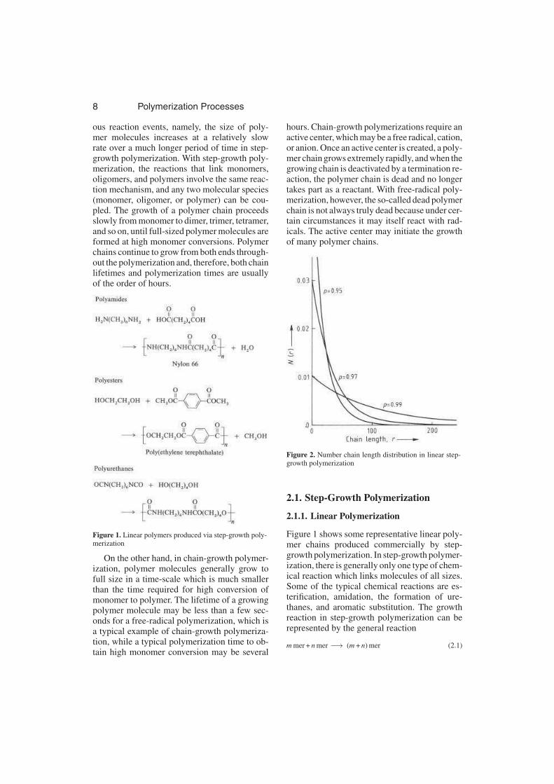
Figure 2. Number chain length distribution in linear step-growth polymerization
2.1. Step-Growth Polymerization
2.1.1. Linear Polymerization
Figure 1 shows some representative linear poly-mer chains produced commercially by step-growth polymerization. In step-growth polymer-ization, there is generally only one type of chem-ical reaction which links molecules of all sizes.Some of the typical chemical reactions are es-terification, amidation, the formation of ure-thanes, and aromatic substitution. The growthreaction in step-growth polymerization can berepresented by the general reaction
m mer + n mer −→ (m + n) mer (2.1)
Polymerization Processes 9
The kinetic study of such reactions would beextremely difficult if the rate constant for thecoupling reaction depended on the size of bothspecies. Fortunately, various kinetic studies haveshown that the rate constant is effectively in-dependent of chain length except perhaps foroligomers. This is often referred to as the con-cept of equal reactivity of functional groups.
Consider the example of step-growth poly-merization shown below.
n A−A + n B−B→——[ A−A−B−B——] n (2.2)
In the case of polyesterification of a diol and adiacid, A may be a hydroxyl group and B maybe a carboxyl group, although the low molecularmass condensation byproduct is not shown. Aswill be shown later, an almost exact equivalencein the number of functional groups is necessaryto obtain polymers with high molecular mass,although a nonstoichiometric condition may beused to control molecular mass. In the case of ex-act stoichiometric ratio of the two types of func-tional groups, i.e., [A] = [B], the polymerizationrate or the rate of disappearance of functionalgroups is given by
−1
V
d (V [A])
dt=K [A]2 (2.3)
except for self-catalyzed polymerization, inwhich case the rate is third order in monomer(the self-catalyzed polymerization may not be auseful reaction from the practical point of viewof productivity). Neglecting the volume changeduring polymerization, integration of Equation(2.3) gives
1/ (1−p) = 1+K [A]0 t (2.4)
where [A]0 is the initial (at t = 0) concentrationof A groups, and p is the conversion of functionalgroups, which is defined as
p=(
NA0−NA
)
/NA0(2.5)
where NA0and NA are the total number of moles
of A groups at t = 0 and at any later time t, respec-tively. Equation (2.4) has been verified by sev-eral kinetic studies. As shown here, the rate ex-pression for a step-growth polymerization is thesame for monomer molecules, oligomers, andpolymers.
The relationship between the average num-ber of structural units (A – A and B – B in the
above example), namely, the number-averagechain length PN and the conversion of func-tional groups p for linear step-growth polymer-ization was first derived by Carothers [20]. PN
is simply given as the total number of monomermolecules initially present divided by the totalnumber of molecules present at time t.
PN =NA0/NA = 1/ (1−p) (2.6)
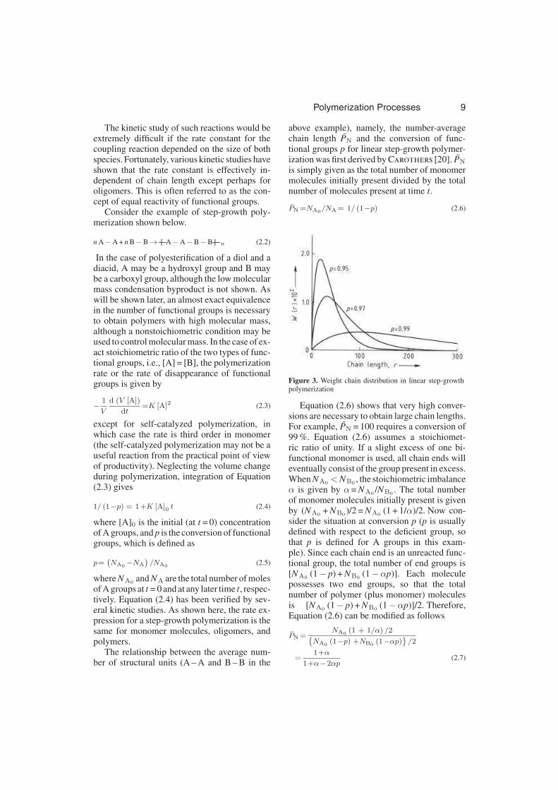
Figure 3. Weight chain distribution in linear step-growthpolymerization
Equation (2.6) shows that very high conver-sions are necessary to obtain large chain lengths.For example, PN = 100 requires a conversion of99 %. Equation (2.6) assumes a stoichiomet-ric ratio of unity. If a slight excess of one bi-functional monomer is used, all chain ends willeventually consist of the group present in excess.When NA0
<NB0, the stoichiometric imbalance
α is given by α = NA0/NB0
. The total numberof monomer molecules initially present is givenby (NA0
+ NB0)/2 = NA0
(1 + 1/α)/2. Now con-sider the situation at conversion p (p is usuallydefined with respect to the deficient group, sothat p is defined for A groups in this exam-ple). Since each chain end is an unreacted func-tional group, the total number of end groups is[NA0
(1− p) + NB0(1−αp)]. Each molecule
possesses two end groups, so that the totalnumber of polymer (plus monomer) moleculesis [NA0
(1− p) + NB0(1−αp)]/2. Therefore,
Equation (2.6) can be modified as follows
PN =NA0
(1 + 1/α) /2{
NA0(1−p) +NB0
(1−αp)}
/2
=1+α
1+α−2αp(2.7)
10 Polymerization Processes
As conversion p approaches unity, PN ap-proaches (1 +α)/(1−α). Thus if α = 0.99, themaximum number-average chain length is only199. This example illustrates the importance ofprecise control of the stoichiometric ratio to ob-tain a desired chain length.
In general, in order to produce high molecularmass polymer by step-growth polymerization,the system must satisfy the following require-ments:
1) Very accurate control of the stoichiometricratio of functional groups
2) Absence of side reactions3) Availability of high-purity monomers4) Reasonably high polymerization rate5) Little tendency towards cyclization reactions
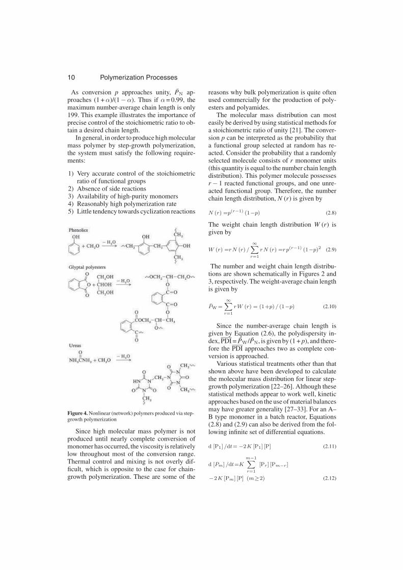
Figure 4. Nonlinear (network) polymers produced via step-growth polymerization
Since high molecular mass polymer is notproduced until nearly complete conversion ofmonomer has occurred, the viscosity is relativelylow throughout most of the conversion range.Thermal control and mixing is not overly dif-ficult, which is opposite to the case for chain-growth polymerization. These are some of the
reasons why bulk polymerization is quite oftenused commercially for the production of poly-esters and polyamides.
The molecular mass distribution can mosteasily be derived by using statistical methods fora stoichiometric ratio of unity [21]. The conver-sion p can be interpreted as the probability thata functional group selected at random has re-acted. Consider the probability that a randomlyselected molecule consists of r monomer units(this quantity is equal to the number chain lengthdistribution). This polymer molecule possessesr− 1 reacted functional groups, and one unre-acted functional group. Therefore, the numberchain length distribution, N (r) is given by
N (r) =p(r−1) (1−p) (2.8)
The weight chain length distribution W (r) isgiven by
W (r) =rN (r) /∞∑
r=1
rN (r) =rp(r−1) (1−p)2 (2.9)
The number and weight chain length distribu-tions are shown schematically in Figures 2 and3, respectively. The weight-average chain lengthis given by
PW =
∞∑
r=1
rW (r) = (1+p) / (1−p) (2.10)
Since the number-average chain length isgiven by Equation (2.6), the polydispersity in-dex, PDI = PW/PN, is given by (1 + p), and there-fore the PDI approaches two as complete con-version is approached.
Various statistical treatments other than thatshown above have been developed to calculatethe molecular mass distribution for linear step-growth polymerization [22–26]. Although thesestatistical methods appear to work well, kineticapproaches based on the use of material balancesmay have greater generality [27–33]. For an A–B type monomer in a batch reactor, Equations(2.8) and (2.9) can also be derived from the fol-lowing infinite set of differential equations.
d [P1] /dt= −2K [P1] [P] (2.11)
d [Pm] /dt=K
m−1∑
r=1
[Pr] [Pm−r]
−2K [Pm] [P] (m≥2) (2.12)

Polymerization Processes 11
where [Pm] is the concentration of polymermolecules with chain length m, and [P] is thetotal concentration of polymer and monomer.
For example, it is straightforward to derivethe molecular mass distribution for the casesin which a slight amount of monofunctionalreagent is used. Kinetic approaches would beeasier to apply to reactors other than batch re-actors, such as semi-batch and continuous flowreactors, although a statistical derivation for astirred-tank reactor has been reported [34].
2.1.2. Interfacial Polymerization
Interfacial polymerization may provide amethod to produce very high molecular masspolymers by step-growth polymerization [35],[36]. In interfacial polymerization, polymers areformed at or in the vicinity of the phase bound-ary of two immiscible monomer solutions. Thistechnique requires an extremely fast polymer-ization. The best reaction type for step-growthpolymerization would be Schotten – Baumannreactions involving acid chlorides. For example,polyamidation is performed at room tempera-ture by placing an aqueous solution of diamineover an organic phase containing the diacidchloride. The polymer formed at the interfacecan be pulled off as a continuous film or fil-ament. The amine – acid chloride reaction rateis so fast that the polymerization becomes dif-fusion controlled. Once the polymer moleculesbegin to grow and monomer molecules start toadd to polymer chain ends, incoming monomermolecules tend to react with polymer chain endsbefore they can penetrate through the polymerfilm to start the growth of new chains. Thus,polymers with much higher molecular massesare formed. Since the reaction is diffusion con-trolled, there is no need to start with an exactbalance of the two monomers. The lower tem-peratures used reduce the relative rates of sidereactions, and, therefore, the purity of monomersis not as important as with most other step-growth polymerizations. In spite of the advan-tages that interfacial polymerization offers, thisprocess has not attracted wide industrial use,mainly because of the high cost of the requiredreactive monomers and the large amount of sol-vent which must be removed and recovered.
2.1.3. Nonlinear Polymerization
Another important class of polymers pro-duced by step-growth polymerization are non-linear polymers formed by polymerization ofmonomers with more than two functional groupsper molecule. Some of the nonlinear polymersproduced commercially by step-growth poly-merization are shown in Figure 4.
In the course of network formation, a polymermolecule of effectively infinite molecular massmay be formed. At this point, termed the gelpoint, the visible formation of a gel or insolublepolymer fraction is observed. The gel moleculeis insoluble in a good solvent even at elevatedtemperatures under conditions at which degrada-tion does not occur. Various physical propertiesof the system change abruptly at the gel point.Gelation should be understood as a critical phe-nomenon having similarities with other criticalphenomena such as vapor – liquid condensation,nuclear chain reactions, and ferromagnetism.
It was Carothers [20], who first derived anequation for the extent of reaction at the gelpoint. He defined a gel molecule as one with infi-nite molecular mass. His criterion that gelationoccurs when the number-average chain lengthPN goes to infinity is not acceptable, since poly-mer molecules larger than PN are always presentand will become gel molecules earlier than thishypothetical gel point. However, the conceptof the “infinitely large molecule” was fully es-tablished by Flory [37–39] using a statisticalapproach. His criterion for the onset of gela-tion is that it occurs when the weight-averagechain length PW goes to infinity. Since a gelmolecule is the largest molecule in the reactionsystem, higher-order moments of the molecu-lar mass distribution could also be used to de-termine the gel point. Fortunately, the second-and higher-order moments approach infinity si-multaneously, at least for batch polymerizations[40], [41], and the criterion of infinite PW is ac-ceptable.
Flory devised a simple tree-like model, asshown in Figure 5, and used the following sim-plifying assumptions:
1) All functional groups of the same type areequally reactive
2) All functional groups react independently ofone another
12 Polymerization Processes
3) No intramolecular reactions occur in finitespecies
Figure 5. A schematic drawing of Flory’s tree-like model(functionality f = 3)The tree-like model is called the Bethe Lattice or Cayleytree by physicists
Figure 6. Molecular mass change and gel growth duringnetwork formation (functionality f = 3)
His basic proposal was that the gel pointis reached when the expectancy of finding thenext generation in a particular existing moleculeis unity. For the tri-functional monomer unitsshown in Figure 5, the conversion at the gelpoint is given by pc = 1/( f− 1) = 0.5, where f isthe functionality of a monomer unit. His modelwas a brilliant development and it provides thestarting point for most theories of polymer net-work formation. A few years later Stockmayer
[42–44] further developed Flory’s idea basedon the most-probable size distribution, and theirtheory is usually called the Flory – Stockmayertheory. Examples of the calculated developmentof the number- and weight-average chain lengthsof the sol fraction and of the weight fractionof gel are shown in Figure 6. Since the gel is
a molecule with many functional groups, the gelonce formed acts like a giant sponge, rapidlyconsuming sol polymer molecules.
This tree-like concept was generalized byGordon et al. [45], [46] based on the theory ofstochastic branching processes, which is consid-ered to be a part of Graph Theory [47], [48]. Thistechnique involves abstract mathematics and re-quires the derivation of the probability generat-ing functions. The method is general but ratherdifficult to use for real problems. To avoid the useof probability generating functions, other prob-abilistic methods have been proposed [49–52].Among them the Macosko – Miller model [50–52] using conditional probabilities is becomingpopular due to its simplicity. All the modelsmentioned above are fully equivalent, that is,only the mathematical language is slightly dif-ferent. These statistical models, which are some-times called the classical theories, have a longhistory and have proven their power of refin-ability to accommodate highly system-specificeffects such as unequal reactivity [53], [54], sub-stitution effects [55], [56], and intramolecularreactions [18], [19], [57–59], which are impor-tant in real systems.
One drawback of the statistical theories men-tioned above is that they assume an equilib-rium system (i.e., the size distribution is calcu-lated anew at each time) and they do not con-sider the kinetic buildup of the system. There-fore, the classical theories may not be appli-cable for kinetically-controlled systems. It hasbeen shown that although there is no differencebetween equilibrium and kinetically-controlledsystems under Flory’s simplifying assump-tions, the difference becomes significant as theconditions deviate further from Flory’s as-sumptions [60], [61], so that in real systems thekinetic features may be dominant. It has beenargued that the kinetic buildup can also be ac-counted for by using a statistical approach [62].
Another disadvantage of statistical ap-proaches may be the excessive modifications re-quired to generalize them for different reactortypes (e.g., continuous reactors). The kineticsapproach was originally shown in the appendixof a paper by Stockmayer [42]. Based on thechemical kinetics, the reaction rate would beproportional to the product of the number of un-reacted functional groups in the respective reac-tion partner, so that an infinite set of differential

Polymerization Processes 13
equations similar to Equations (2.11) and (2.12)can be set up. This idea has been applied to poly-meric systems [60], [63–70].
Figure 7. Example of percolation at the gel point in a squarelattice (pc = 0.5) [78]
All the theories mentioned above belong to amean-field theory. On the other hand, the perco-lation theory [71–77], which is considered to beequivalent to a non-mean-field theory, has beenapplied to polymeric gelation [78], [79]. The per-colation theory is usually associated with a lat-tice model to describe network structure. Oneof the simplest examples is the two-dimensionallattice shown in Figure 7. In this figure, eachbond which has been formed is shown as ashort line connecting two monomers, though themonomers are not shown. In the random (stan-dard) percolation theory each site of a very largelattice is occupied randomly with probabilityp, independent of its neighbors. Some nearly“infinite” molecules can be seen in Figure 7,where “infinite” means that they span the wholesample. Mathematical methods to calculate thisthreshold exactly are restricted so far to two di-mensions [77], and therefore, for practical cal-culations the Monte Carlo simulation is usuallyused. It is easy to understand why gelation isa critical phenomenon from the lattice model,because in the vicinity of the gel point only afew additional bonds are necessary to form amolecule which spans the whole sample. Thepercolation theory emphasizes the universalityof critical phenomena and space dimensional-
ity. De Gennes wrote in his book [80] that “ittook more than thirty years to convince exper-imentalists that mean-field theory was wrong”.However, at present the percolation models arefar from simulating actual network formationquantitatively, because the bonds are too rigid,the movement of molecules is too suppressed,and necessary chemical rules of bond formationare ignored. The percolation theory is essentiallydevoted to describing the behavior near the criti-cal threshold pcr, where the system-specific fea-tures are not important.
Network polymers are increasingly used asengineering materials because of their excellentstability toward elevated temperature and physi-cal stress. Since the three-dimensional polymersare neither soluble nor fusible once made, the fi-nal stage of polymerization is usually carried outin a mold of the desired shape.
2.2. Chain-Growth Polymerization
Chain-growth polymerization is initiated by areactive species, R∗in, produced from an initiatoror catalyst I.
I−→ n R∗in (2.13)
Depending on the type of active center, chain-growth polymerization can be divided into free-radical, anionic, and cationic polymerization.The reactive species R∗in adds to a monomerto form a new active center, and monomermolecules are added to the active center suc-cessively. This process is called the propagationreaction:
where M represents a monomer molecule, andP∗r is an active polymer molecule with chainlength r. In general, the propagation reaction isrepresented by
In chain-growth polymerization, onlymolecules with an active center can propa-gate, so that polymer molecules once formedmay be considered dead polymer for linearchain-growth polymerization. Dead polymer

14 Polymerization Processes
molecules do not take part as reactants there-after. The active center is always on the chainend when linear chains are being produced ex-clusively. Polymer chain growth is terminated atsome point by unimolecular and/or bimoleculartermination. Bimolecular termination of activecenters occurs only in free-radical polymeriza-tion.
Carbon – carbon double bonds and thecarbon – oxygen double bond in aldehydes andketones are the two main types of func-tional groups which undergo chain-growthpolymerization. The polymerization of thecarbon – carbon double bond is much more im-portant, as most commercial monomers withcarbon – carbon double bonds readily undergofree-radical polymerization (an important ex-ception is propene). The carbonyl bond is notgenerally susceptible to polymerization by rad-ical initiators due to its highly polarized struc-ture. Another reason is that most of the carbonylmonomers (except formaldehyde) possess verylow ceiling temperatures [81], [82] (the tempera-ture above which active polymer chains depoly-merize rather than grow).
Most of the commercial vinyl monomers(CH2=CHX and CH2=CXY, and monomers inwhich fluorine is substituted for hydrogen) canbe polymerized with free radicals. Whether avinyl monomer can be polymerized by anionicor cationic mechanisms strongly depends onthe type of monomer. Monomers with electron-donating groups attached to the doubly bondedcarbon atoms form stable carbenium ions andpolymerize best with cationic initiators. Con-versely, monomers with electron-withdrawingsubstituents form stable carbanions and requireanionic initiators. It should be noted that ionsof low stability would be expected to react withcarbon – carbon double bonds; however, in manycases they cannot be formed or else are easilyconsumed by side reactions.
2.2.1. Free-Radical Polymerization
Generally, free-radical polymerization consistsof four types of elementary reaction.
1) Initiation reactions, which continuously gen-erate radicals during polymerization.
The stoichiometric coefficient n is two forthermal decomposition of initiators. A free-
radical R•
in derived from the initiator is calleda primary or initiator radical.
2) Propagation reactions, which are responsiblefor the growth of polymer chains by additionof monomer to a radical center.
3) Bimolecular termination reactions betweentwo radical centers, which give a net con-sumption of radicals. These consist of dis-proportionation (Eq. 2.19) and combination(Eq. 2.20).
where Pr is a polymer molecule of chainlength r and does not have a radical center,while a polymer radical (or macroradical) of
chain length r has the symbol R•
r .4) Chain transfer to small molecules which
causes the cessation of growth of poly-mer radicals while generating small trans-fer radicals simultaneously. Chain-transferreactions do not give a net consumption ofradicals, and if the transfer radicals are asreactive as polymer radical (or more reac-tive) these reactions should not affect thepolymerization rate or monomer consump-tion rate when the bimolecular terminationreactions are chemically controlled. Chain-transfer reactions to small molecules re-duce the size of polymer radicals and there-fore would increase bimolecular terminationrates when these reactions are diffusion con-trolled (bimolecular termination rates maybe chain-length dependent under these con-ditions).
Polymerization Processes 15
X may be monomer, a solvent molecule, ora chain-transfer agent. When X is a poly-mer molecule, polymer molecules with long-chain branches are formed. Long-branch for-mation is discussed in Section 2.2.1.7.
The sequence of elementary reactions, inEquations (2.16) – (2.22) results in total radicalconcentrations of the order 10−9 – 10−5 mol/Lfor most commercial polymerizations. Sincepolymer molecules with high molecular massesare produced from the very start of polymeriza-tion, the reacting solution can be quite viscousover most of the monomer conversion range. Thehigh viscosities not only cause problems in mix-ing and heat removal, but also can affect reactionrates (reactions such as bimolecular terminationof polymer radicals). This topic is discussed inSection 2.2.1.3.
Free-radical polymerization is the most com-monly used method for the synthesis of poly-mers from vinyl and divinyl monomers. Sometypical monomers which readily undergo free-radical polymerization are ethylene, styrene,vinyl chloride, vinylidene chloride, acryloni-trile, vinyl acetate, methyl methacrylate, methylacrylate, acrylamide, etc. Of all chain-growthpolymerization processes, it is the most widelystudied and best understood.
2.2.1.1. Initiation
Free radicals may be generated in a monomer ina number of ways. The most often used method isto add chemical initiators, such as azo and perox-ide compounds, to the monomer in low concen-trations (usually < 1 wt % based on monomer).When heated, the initiator decomposes, gener-ating radicals which act as active centers formonomer addition. For example, organic per-oxides (ROOR′) decompose thermally by O – Obond cleavage to produce two initiator radicalsas follows (other side reactions may of courseoccur).
where Kd is a thermal decomposition rate con-stant with units of inverse time, most often s−1.For a batch reactor, the change in the number ofmoles of initiator N I is given by
dNI/dt= −KdNI (2.24)
For isothermal decomposition (isothermal poly-merization) Equation (2.24) can be integratedanalytically to obtain
NI =NI0 exp (−Kdt) (2.25)
where N I0 is the number of moles of initiator attime t = 0.
Thus the half-life of an initiator is given by
t1/2 = − ln (0.5) /Kd = 0.693/Kd (2.26)
Knowledge of Kd for an initiator therefore per-mits calculation of the initiator half-life t1/2.Since Kd has an Arrhenius temperature depen-dence, Kd and t1/2 both depend on temperature.
Activation energies for peroxides and azo ini-tiators are ca. 120 kJ/mol, so the decompositionrate is highly temperature dependent, and theuseful temperature range is quite small (decom-position rate is either too fast or too slow outsidethe useful temperature range, which normallyspans about 30 ◦C).
To complete the initiation step, the initiator
radicals (R•
in ) must add to the double bond of amonomer molecule to generate a polymer radi-
cal of unit chain length R•
l . In most polymeriza-tions, this step (Eq. 2.17) is much faster than therate of initiator decomposition (Eq. 2.16). Thehomolysis of the initiator is the rate-determiningstep in the initiation sequence, and the initiationrate RI is given by
RI = 2Kdf [I] (2.27)
where f is the initiator efficiency. The initiatorefficiency is defined as the fraction of radicalsproduced by initiator decomposition that initiatepolymer radicals. Note that not every initiatormolecule, which in principle can produce twopolymer radicals, does so. Some primary rad-icals may react with themselves or with othermolecules to form stable species which do notform either polymer radicals or molecules. Itshould be noted that chain transfer to the initia-tor does not decrease f . The initiator efficiency

16 Polymerization Processes
usually has values in the range 0.2 – 1.0 at lowmonomer conversions, where polymer concen-trations are low. The major cause of low ini-tiator efficiency is recombination of the radicalpairs before they diffuse apart, which is calledthe cage effect [83], [84]. When an initiator de-
composes, the primary radicals R•
in are near-est neighbors for about 10−10 – 10−9 s. Duringthis interval they are surrounded by a “cage” ofsolvent and monomer molecules through whichthey must diffuse to escape from the cage. Sincereactions between radicals are extremely fast,there is reasonable probability that reaction bet-ween primary radicals occurs. Direct recombi-nation may simply regenerate the original initia-tor molecules, but other reactions can also occurthat consume initiator radicals without formingpolymer chains. In particular, since azo initiatorsdecompose with the elimination of a nitrogenmolecule, recombination of the primary radicalsresults in the formation of a stable molecule thatcannot generate radicals, and thus there may bea significant decrease in initiator efficiency. Ef-ficiency decreases with increasing viscosity ofthe reaction medium [85], [86]. Thus f decreasesduring the course of polymerization and may ap-proach zero at very high polymer concentrationswhere the diffusion coefficient of primary radi-cals in the “cage” is very small [87], [88].
When selecting an initiator type, in generalone needs to consider the decomposition rateconstant, water and oil solubility, stability of ini-tiator fragments on chain ends, and other factors.Another important point is the activity of the ini-tiator radical center towards the abstraction ofatoms (e.g., hydrogen atoms) from the polymerbackbone. This can lead to chain scission, long-chain branching, and possibly cross-linking.
Up to this point, only monofunctional ini-tiators (initiators with one peroxide or oneazo group per molecule) have been consid-ered. There are commercially available bifunc-tional initiators (with two peroxide groups permolecule) with some potentially useful applica-tions [89–92]. Their function can be illustratedas follows:
Even when the Kd’s for both peroxide groupsare the same, both groups on the same peroxidemolecule do not decompose at the same time;thus a significant fraction of the polymer chainswill have a peroxide end group. These terminalperoxide groups will later decompose, generat-ing polymer radicals with an initiator fragmentin the backbone. The practical benefits includehigher molecular masses at the same tempera-ture or comparable molecular masses at highertemperatures. Polymerization at higher temper-atures results in higher productivity. These ben-efits will only accrue when most of the poly-mer chains are formed by bimolecular termina-tion of polymer radicals. When chain transferto small molecules produces most of the poly-mer chains, these benefits will no longer exist,and since bifunctional initiators are more expen-sive than monofunctional initiators it is recom-mended that the latter be used.
The decomposition rates of peroxy and azocompounds can be increased by irradiation withultraviolet and visible light. Unlike thermaldecomposition, the activation energy for pho-tochemical initiation is approximately zero, sopolymerization can be initiated at much lowertemperatures. Compounds such as benzoin anddisulfides, whose bonds are too strong to un-dergo thermal homolysis, are effective radicalinitiators under ultraviolet irradiation. Photo-chemical polymerization has been applied incoatings and inks for metal, paper, wood andplastics, in photo-imaging, printing circuits, andadhesives, although its use is limited by low pen-etration into the polymerizing mass.
Another method of lowering the activationenergy of the peroxide decomposition reactionis to use redox initiation systems. The additionof a reducing agent results in radical formationfrom an oxidation – reduction reaction betweenthe two components. Generally, the reaction isillustrated as follows.
An+ + ROOR′−→A(n+1)+ + R′O•
+ RO− (2.29)
where A is a reducing agent and ROOR′ is a per-oxide. The integer n is two for Fe2+ and zero forN,N-dimethylaniline. The fate of the free radicaldepends on the relative concentration of reduc-ing agent and monomer. Since the redox initiatonreactions do not produce a pair of radicals, thecage effect is not operative. At high monomer
Polymerization Processes 17
concentrations most of the free radicals initi-ate polymerization, and ordinary second-orderkinetics are obeyed. Redox initiation is usuallyused in the temperature range 0 – 50 ◦C.
All methods mentioned above employ initia-tors. There are, however, other means to initiatepolymerization. Styrene (and some substitutedstyrenes such as p-methylstyrene) and methylmethacrylate polymerize at elevated tempera-tures in the absence of a free-radical initiat-ing system. The accepted mechanism for ther-mal initiation of styrene is the Mayo mecha-nism [93], [94], which involves the formationof a Diels – Alder dimer intermediate which re-acts with styrene to produce radicals. The Mayomechanism is consistent with an observed initi-ation rate which can vary from second to thirdorder in monomer during the course of polymer-ization [95–97], and some confirming evidencehas been reported [98–100]. A serious disadvan-tage of the use of thermal initiation for styrene isthe formation of undesirable byproducts (cyclicdimers and trimers) which are difficult to removeto give a high-quality polystyrene.
Irradiation with UV, high-energy electrons,and γ-rays can initiate polymerization withor without the presence of initiators. Radia-tion initiation has been used almost exclusivelyfor polymer modification (chain scission, long-chain branching, cross-linking, and grafting).These radiation processes are characterized bya zero activation energy for radical generationand as a consequence a low activation energyfor polymerization. Therefore, they are effectiveat both low and high temperatures. With radi-ation initiation, polymer molecular masses in-crease with increasing temperature, which is op-posite to that for chemically initiated free-radicalpolymerizations (the high activation energy forinitiator decomposition is responsible for this).Both UV and electrons have small penetrationdepths and are therefore used for polymeriza-tions in thin layers. Gamma rays have highpenetration depths but require expensive safetyinstallations. Radiation polymerization may beinitiated by radicals, cations, or anions. The ef-fectiveness of a radical center depends on thechemistry of the monomer and the polymeriza-tion conditions. Most radiation polymerizationsare free-radical except at very low temperatureswhere ionic species are sufficiently stable. Withradiation initiation various active intermediates
may be formed, leading to a very complex reac-tion mixture with the formation of many byprod-ucts as well as the formation of long branchesand possibly cross-linkages. Since photon ener-gies for UV are lower, UV radiation generallygives cleaner polymerizations with the forma-tion of linear chains, although monomers whichundergo photolysis by UV radiation are limited.
2.2.1.2. Propagation
The propagation reaction (Eq. 2.18) controlsboth the rate of growth and the structureof the polymer chain. Monomers which un-dergo free-radical polymerization are com-monly monosubstituted or 1,1-disubstituted eth-ylenes, CH2=CHX or CH2=CXY. With 1,1-di-substituted ethylenes both substituents shouldnot be large, since propagation would be ster-ically hindered. 1,2-Disubstituted ethylenes arenormally considered very difficult to polymer-ize since the approach of the propagating rad-icals to a monomer is sterically hindered. 1,2-Disubstituted ethylenes can, however, often beincorporated into copolymers.
Due to steric and resonance effects, vinylmonomers predominantly undergo head-to-tailaddition:
In certain cases when the substituents aresmall and do not have large resonance stabiliz-ing effects, head-to-head propagation may oc-cur. For example, approximately 16 % head-to-head placement has been reported for poly(vinylfluoride) [101].
In free-radical polymerization, chain mi-crostructure is largely independent of initiationmechanism and initiator type. Polymers pro-duced by free-radical polymerization are largelyatactic, since the terminal carbon – carbon bondcan rotate freely during chain growth. The con-figuration of a monomer unit in the chain isnot determined during its addition to the rad-ical center but only when the next monomermolecule adds to it. The slight preference forsyndiotactic over isotactic placement is causedby steric and/or electrical repulsion between
18 Polymerization Processes
substituents in the chain, although at high tem-peratures their effects are progressively dimin-ished. For example, the fraction of syndiotacticdiads of poly(vinyl chloride) changes from 0.67to 0.51 as the synthesis temperature increasesfrom− 78 ◦C to 120 ◦C [102]. For methyl meth-acrylate, it is 0.86 at− 40 ◦C and 0.64 at 250 ◦C[103], [104].
For most chain-growth polymerizations(free-radical or ionic) the propagation reactionsare reversible at elevated temperature and therate of depropagation is significant [105], [106].
where Kdp is the rate constant for depolymeriza-tion (depropagation). The ceiling temperatureT c, which is the temperature above which activepolymer chains depolymerize rather than grow,is reached when the propagation and depropa-gation rates are equal. Based on thermodynamicarguments, the ceiling temperature can be re-lated to the equilibrium monomer concentration[M]c as follows:
Tc = ∆H/(
∆S0 +R ln [M]c)
(2.32)
where ∆H is the heat of polymerization, ∆S0
the entropy change of polymerization at unitmonomer concentration, and R the gas constant.
The ceiling temperature T c is not a singu-lar value but is a function of monomer con-centration. At any temperature, a concentra-tion of monomer exists at which the reactionin Equation (2.31) is at equilibrium. The exis-tence of this equilibrium concentration preventsmonomer conversion reaching 100 %.
Normally, this equilibrium monomer concen-tration is too low to detect. A notable exception isα-methylstyrene whose T c for 100 % monomerconcentration is 61 ◦C, and the equilibriummonomer concentration at 25 ◦C is 2.2 mol/L[107].
Conventionally, it has been assumed that thepropagation rate constant Kp is independent ofchain length. Experimental results have shownthat Kp is independent of chain length at leastfor chain lengths > 16 for styrene and > 62 formethyl methacrylate [108]. The propagation rateconstant Kp is relatively insensitive to the vis-cosity of the system except at very high polymerconcentrations [88], [109].
It has long been recognized that some bulkpolymerizations stop at well below 100 % con-version [110]. This phenomenon has success-fully been explained as due to a glassy-state tran-sition of the polymerizing mass [111]. Althoughthe polymerization can proceed very slowly inthe glassy state [109], [112], for practical pur-poses it can be assumed that polymerizationstops when the system changes from a viscousliquid to a solid glass. It has been proposed thatthe initiator efficiency f approaches zero whenthe system reaches a glassy state [87], [113] andthat this is mainly responsible for the cessationof polymerization.
2.2.1.3. Termination
An active center on a growing polymer radicalmay be destroyed by a variety of processes, in-cluding termination by added substances. Thelatter reactions are called inhibition and retarda-tion processes, and are not considered here. Thissection discusses bimolecular termination reac-tions between polymer radicals. Although oneof the radicals involved in bimolecular termina-tion may be an initiator radical, under normalpolymerization conditions such reactions maybe negligible since the concentration of initiatorradicals is much smaller than that of polymerradicals.
Bimolecular termination of two polymer rad-icals can occur by combination or coupling:
or by disproportionation, in which case a hy-drogen radical is transferred from one polymerchain to the other. The result is the formationof two polymer molecules, one of which has aterminal double bond.
Termination by combination and dispropor-tionation can occur simultaneously, and the rel-ative importance of these two modes of termi-
Polymerization Processes 19
nation depends on monomer type and polymer-ization temperature. Experimental data are notavailable for many monomers; however, radicalswhich undergo termination by combination ap-pear exclusively to have the structure (1) [114].A well-known example is styrene, which experi-ences termination by combination almost exclu-sively over a wide range of temperatures [114],[115]. On the other hand, radicals which undergodisproportionation and combination may havethe structure (2).
For methyl methacrylate, combination and dis-proportionation are both important at low tem-perature, with disproportionation becoming thedominant mode at high temperatures [116–118].
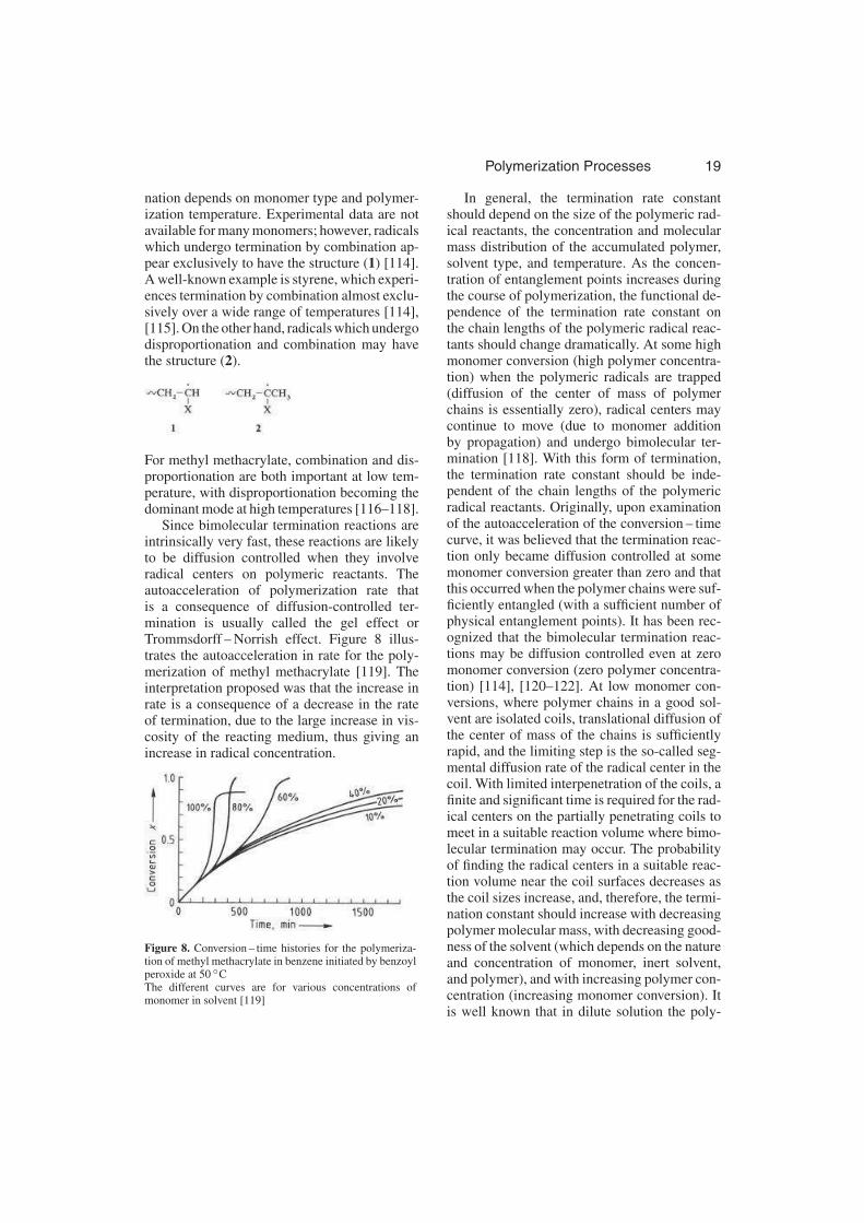
Since bimolecular termination reactions areintrinsically very fast, these reactions are likelyto be diffusion controlled when they involveradical centers on polymeric reactants. Theautoacceleration of polymerization rate thatis a consequence of diffusion-controlled ter-mination is usually called the gel effect orTrommsdorff – Norrish effect. Figure 8 illus-trates the autoacceleration in rate for the poly-merization of methyl methacrylate [119]. Theinterpretation proposed was that the increase inrate is a consequence of a decrease in the rateof termination, due to the large increase in vis-cosity of the reacting medium, thus giving anincrease in radical concentration.
Figure 8. Conversion – time histories for the polymeriza-tion of methyl methacrylate in benzene initiated by benzoylperoxide at 50 ◦CThe different curves are for various concentrations ofmonomer in solvent [119]
In general, the termination rate constantshould depend on the size of the polymeric rad-ical reactants, the concentration and molecularmass distribution of the accumulated polymer,solvent type, and temperature. As the concen-tration of entanglement points increases duringthe course of polymerization, the functional de-pendence of the termination rate constant onthe chain lengths of the polymeric radical reac-tants should change dramatically. At some highmonomer conversion (high polymer concentra-tion) when the polymeric radicals are trapped(diffusion of the center of mass of polymerchains is essentially zero), radical centers maycontinue to move (due to monomer additionby propagation) and undergo bimolecular ter-mination [118]. With this form of termination,the termination rate constant should be inde-pendent of the chain lengths of the polymericradical reactants. Originally, upon examinationof the autoacceleration of the conversion – timecurve, it was believed that the termination reac-tion only became diffusion controlled at somemonomer conversion greater than zero and thatthis occurred when the polymer chains were suf-ficiently entangled (with a sufficient number ofphysical entanglement points). It has been rec-ognized that the bimolecular termination reac-tions may be diffusion controlled even at zeromonomer conversion (zero polymer concentra-tion) [114], [120–122]. At low monomer con-versions, where polymer chains in a good sol-vent are isolated coils, translational diffusion ofthe center of mass of the chains is sufficientlyrapid, and the limiting step is the so-called seg-mental diffusion rate of the radical center in thecoil. With limited interpenetration of the coils, afinite and significant time is required for the rad-ical centers on the partially penetrating coils tomeet in a suitable reaction volume where bimo-lecular termination may occur. The probabilityof finding the radical centers in a suitable reac-tion volume near the coil surfaces decreases asthe coil sizes increase, and, therefore, the termi-nation constant should increase with decreasingpolymer molecular mass, with decreasing good-ness of the solvent (which depends on the natureand concentration of monomer, inert solvent,and polymer), and with increasing polymer con-centration (increasing monomer conversion). Itis well known that in dilute solution the poly-

20 Polymerization Processes
mer coil size decreases with increasing polymerconcentration.
At somewhat higher conversions, when thereare a sufficient number of chain entanglementpoints, the translational diffusion rate of the cen-ter of mass of polymer coils decreases dramati-cally and bimolecular termination rates becometranslationally diffusion controlled. Of course,shorter polymer chains will experience transla-tional diffusion-controlled termination at highermonomer conversions (higher polymer concen-trations) than longer chains, and clearly thebimolecular termination rate constant will bechain-length dependent and the bivariate distri-bution Kt (r, s) will change its shape dramat-ically with increasing polymer concentration.Finally, when the polymer coils are trapped,Kt should become independent of chain length[118].
Figure 9. Polymerization of acrylamide – rate and molec-ular mass development (T = 60 ◦C, [M]0 = 3.4 mol/L, initi-ated by potassium peroxosulfate [I]0 = 5.2× 10⁻⁴ mol/L)– – – = Constant Kt; —- = Use of Equation (2.35) [126]
The mechanisms of diffusion-controlled re-actions in polymer systems are being clari-fied both theoretically and experimentally (seefor example [122]), but at present developinga general formulation for Kt for the wholecourse of polymerization is a formidable task.Considering the complexity of the mechanismsof diffusion-controlled termination reactions, insome cases it may be necessary to use an empir-ical approach for reactor calculations [96], [97],[123–126]. For example, Kt may be approxi-mated by
Kt =Kt0 exp[
−(
A1x+A2x2 +A3x
3)]
(2.35)
where x is the monomer conversion, Kt0 isthe termination rate constant at zero monomerconversion (x = 0), and A1, A2, A3 are ad-justable parameters. An application is shownin Figure 9. The adjustable parameters A1, A2,A3 are usually estimated by fitting isothermalconversion – time curves. The adjustable param-eters should be functions of temperature andpossibly initiator concentration (radical initia-tion rate). Note that Kt estimated by fitting poly-merization rate and number-average molecularmasses is a number-average termination rateconstant. Although, this termination rate con-stant may predict rates of polymerization andnumber-average molecular masses adequately,its use to calculate higher averages will under-estimate weight-average, and Z-average molec-ular mass [88].
Figure 10. Effect of inhibitors and retardersa) No retarder or inhibitor ; b) With retarder; c) With in-hibitor
2.2.1.4. Chain Transfer to Small Molecules
During free-radical polymerization, chain trans-fer to small molecules X may occur. The smallmolecule may be initiator, monomer, chain-transfer agent, solvent, inhibitor, or impurity. Ingeneral, these chain-transfer reactions can be re-presented by Equations (2.21) and (2.22).

Polymerization Processes 21
When K ′p is approximately zero (i.e., X•
is a
stable radical) X is called an inhibitor. If K ′p issmaller than the propagation rate constant Kp,X is called a retarder. Idealized behavior of in-hibitors and retarders is shown schematically inFigure 10. The kinetics of inhibition and retar-dation can be found elsewhere [127].
For an added agent to be a chain-transferagent, K ′p must be approximately equal to Kp
(or Kp<K ′p, if chain length is large enough).Therefore, the chain-transfer agent reduces themolecular masses but does not affect rates ofpolymerization.
The chain-transfer rate constants for mostmonomers are about 104–105 times smaller thanthe propagation rate constant (K fm/Kp = 10−5–10−4).
The presence of monomer molecules is in-evitable, so that the value of K fm/Kp places anupper limit on the polymer molecular mass thatcan be obtained with a given monomer. LargerK fm values are observed when the propagatingradicals have very high energies (high reactivi-ties), such as in the case of ethylene, vinyl ac-etate, and vinyl chloride.
2.2.1.5. Kinetics of Linear Polymerization
The elementary reactions involved in linear free-radical polymerization (chains produced are lin-ear with no branches or cross-links) are as fol-lows:Initiation
Propagation
Chain transfer to monomer
Chain transfer to small molecule (T)
Termination by disproportionation
Termination by combination
To derive the kinetic rate equations, the fol-lowing assumptions are usually made:
1) All rate constants are independent of chainlength.
2) Chain lengths are sufficiently large that thetotal rate of monomer consumption may beequated to the rate of monomer consump-tion by the propagation reactions alone [thisis often called the long-chain approximation(LCA)].
3) Radicals generated in chain-transfer reac-tions propagate with monomer rapidly andthus do not affect the polymerization rate.
4) The stationary-state hypothesis (SSH) isvalid for radical reactions. One can thereforeassume that both the rates of radical genera-tion and consumption are much greater thanthe rate of change of radical concentrationwith respect to time [128], [129].
Let us first derive an expression for the poly-merization rate Rp, applying the above assump-tions. The balanced equation for polymer radi-cals with chain length r is given by
1
V
d(
V[
R·
l
])
dt= RI +Kfm [M]
∞∑
r=2
[R·
r]
+K′p [T·] [M] −KfT [R·
1] [T] −Kp [R·
1] [M]
− (Ktc +Ktd) [R·
1] [R·] (2.36)
1
V
d (V [R·
r])
dt=Kp
[
R·
r−1
]
[M] −Kp [R·
r] [M]
−Kfm [R·
r] [M] −KfT [R·
r] [T]
− (Ktc +Ktd) [R·
r] [R·] (r≥2) (2.37)
where RI is the initiation rate (RI = 2 Kd f [I])
and [R·] =∞∑
r=1
[R·
r], which is the total polymer
radical concentration. The transfer radical con-centration [T
•
] is given by

22 Polymerization Processes
1
V
d (V [T·])
dt=KfT [R·] [T] −K′p [T·] [M] (2.38)
Applying the stationary-state hypothesis gives
KfT [R·] [T] =K′p [T·] [M] (2.39)
Summation of Equations (2.36) and (2.37) overall chain lengths (1 to infinity) and substitutingEquation (2.39) into the sum gives
1
V
d (V [R·])
dt=
∞∑
r=1
1
V
d (V [R·
r])
dt
=RI+K′p [T·] [M]−KfT [R·] [T]− (Ktc+Ktd) [R·]2
=RI − (Ktc+Ktd) [R·]2 (2.40)
Application of the stationary-state hypothesis
for the total polymer radical concentration [R•
],gives
RI =Kt [R·]2 (2.41)
where Kt = Ktc + Ktd. In the above formalism,the termination rate, Rt is given by
Rt =Kt [R·]2 (2.42)
It is worth noting here that Rt = 2 Kt [R•
]2 is of-
ten used in the literature, although Rt = Kt [R•
]2
is more widely used in free-radical polymeriza-tion (e.g., the compilation of kinetic rate con-stants in [130]). One must distinguish carefullywhich type of termination rate constant is beingused when consulting the literature on polymer-ization kinetics.
From Equation (2.41), the total polymer rad-ical concentration is given by
[R·] = (Rl/Kt)0.5 (2.43)
Based on the long-chain approximation, thepolymerization rate Rp is given by
Rp = −1
V
d (V [M])
dt=Kp [R·] [M]
=
(
Kp
K0.5t
)
R0.5I [M] (2.44)
Since RI= 2Kdf [I] ,
Rp =
(
Kp
K0.5t
)
(2Kdf [I])0.5 [M] (2.45)
Equation (2.45) predicts a first-order depen-denceon monomer concentration and a square-root dependence on initiator concentration, the
latter being a direct consequence of the bimo-lecular nature of the termination reaction.
Now consider the weight chain length dis-tribution W (r). Application of the stationary-state hypothesis for polymer radicals with chainlength r (Eq. 2.36 and 2.37) gives.
[R·
l ] (2.46)
=RI +Kfm [M] [R·] +KfT [T] [R·]
Kp [M] +Kfm [M] +KfT [T] + (Ktc +Ktd) [R·]
[R·
r] (2.47)
=Kp [M]
[
R·
r−1
]
Kp [M] +Kfm [M] +KfT [T] + (Ktc +Ktd) [R·]
Let us introduce the following dimensionlessgroups:
τ=Rtd +Rf
Rp=Ktd [R·] +Kfm [M] +KfT [T]
Kp [M](2.48)
β=Rtc
Rp=Ktc [R·]
Kp [M](2.49)
where
Rp = Kp [R•
] [M]; propagation rate
Rtd = Ktd [R•
]2 ; rate of termination by dis-proportionation
Rtc = Ktc [R•
]2 ; rate of termination by com-binationRf = K fm [R
•
] [M] + K fT [R•
] [T]; rate ofchain transfer.
Since RI = Rtd + Rtc, Equations (2.46) and(2.47) can be simplified as follows:
[R·
1] =τ+β
1+τ+β[R·] (2.50)
[R·
r] =1
1+τ+β
[
R·
r−1
]
(2.51)
Therefore,
[R·
r] = [R·] (τ+β)Φr (2.52)
where
Φ= 1/(1 + τ +β)
Now consider the production rate of polymermolecules with chain length r, RFP (r), which isgiven by

Polymerization Processes 23
RFP (r) =1
V
d (V [Pr])
dt
= (Kfm [M] +KfT [T] +Ktd [R·]) [R·
r]
+1
2Ktc
r−1∑
s=1
[R·
s][
R·
r−s
]
(2.53)
Substituting for [R•
r ] using Equation (2.52) gives
RFP (r) (2.54)
=Kp [R·] [M] (τ+β)
{
τ+β
2(τ+β) (r−1)
}
Φr
The instantaneous weight chain length distribu-tion W (r) is therefore given by
W (r) =rRFP (r)∞∑
r=1rRFP (r)
=(τ+β)
{
τ+ β2
(τ+β) (r−1)}
rΦr
1+τ+β
= (τ+β)
{
τ+β
2(τ+β) (r−1)
}
rΦr+1 (2.55)
Ifβ≪ τ , that is most polymer chains are formedby chain transfer and/or termination by dispro-portionation, Equation (2.55) reduces to
W (r) =τ2rΦr+1 =r
(
1
1+τ
)r−1 (
τ
1+τ
)2
(2.56)
Here, 1/(1 + τ ) is the probability of growth fora given polymer radical, and τ /(1 + τ ) is theprobability that a polymer radical stops grow-ing. Therefore, Equation (2.56) is essentially thesame as the distribution derived for linear step-growth polymerization (Eq. 2.9), based on a sta-tistical argument.
It is sometimes more convenient to describethe chain length distribution as a continuousfunction rather than a discrete function, and thiscan often be done with small error as r is usuallyvery large. Therefore, the following approxima-tion may be useful:
W (r)≈ (τ+β)
{
τ+β
2(τ+β) (r−1)
}
r
·exp {− (τ+β) r} (2.57)
Note that (τ +β) has the value of ca. 10−6–10−2 for usual free-radical polymerization[(τ +β)≪ 1].
The weight-average chain length PW forpolymer produced instantaneously is given by
PW =
∞∑
r=1
rW (r) =τ (2+τ+β) +β (3+τ+β)
(τ+β)2
≈2τ+3β
(τ+β)2(2.58)
The instantaneous number-average chain lengthPN is given by
PN =1
∞∑
r=1W (r) /r
=(1+τ+β)
(τ+β/2)≈
1
(τ+β/2)(2.59)
The polydispersity index PDI for polymer pro-duced instantaneously is given by
PDI =PW
PN≈
(2τ+3β) (τ+β/2)
(τ+β)2(2.60)
If β = 0, i.e., termination by combination doesnot occur, the polydispersity index takes on themaximum value, PDI = 2. On the other hand, ifτ = 0, i.e., chain termination is solely by bimo-lecular termination through combination, PDItakes on the minimum value, 1.5. Figure 11shows the PDI as a function of the fraction ofchain termination by bimolecular termination bycombination, β/(τ +β).
Figure 11. Effect of the type of chain termination on thepolydispersity index
The W (r), PW, PN, and PDI derived heregive the instantaneous properties. In linear free-radical polymerization the polymer moleculesonce formed are inert and do not react further.
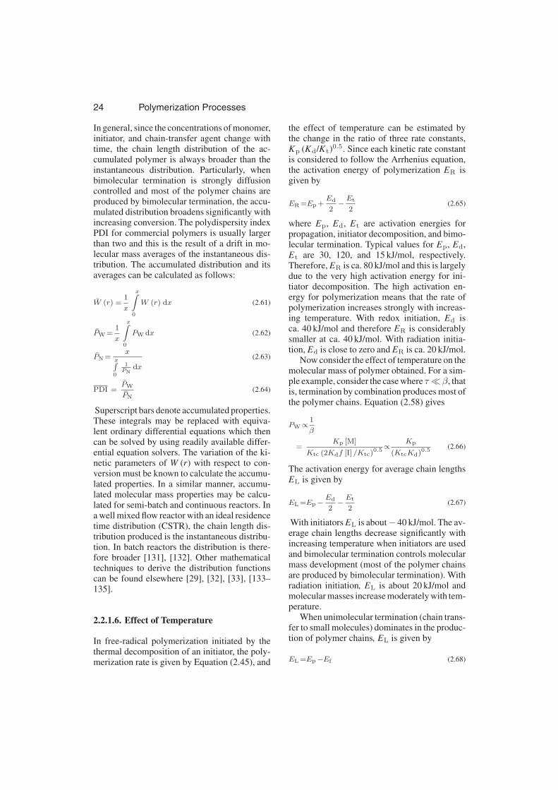
24 Polymerization Processes
In general, since the concentrations of monomer,initiator, and chain-transfer agent change withtime, the chain length distribution of the ac-cumulated polymer is always broader than theinstantaneous distribution. Particularly, whenbimolecular termination is strongly diffusioncontrolled and most of the polymer chains areproduced by bimolecular termination, the accu-mulated distribution broadens significantly withincreasing conversion. The polydispersity indexPDI for commercial polymers is usually largerthan two and this is the result of a drift in mo-lecular mass averages of the instantaneous dis-tribution. The accumulated distribution and itsaverages can be calculated as follows:
W (r) =1
x
x∫
0
W (r) dx (2.61)
PW =1
x
x∫
0
PW dx (2.62)
PN =x
x∫
0
1PN
dx
(2.63)
PDI =PW
PN(2.64)
Superscript bars denote accumulated properties.These integrals may be replaced with equiva-lent ordinary differential equations which thencan be solved by using readily available differ-ential equation solvers. The variation of the ki-netic parameters of W (r) with respect to con-version must be known to calculate the accumu-lated properties. In a similar manner, accumu-lated molecular mass properties may be calcu-lated for semi-batch and continuous reactors. Ina well mixed flow reactor with an ideal residencetime distribution (CSTR), the chain length dis-tribution produced is the instantaneous distribu-tion. In batch reactors the distribution is there-fore broader [131], [132]. Other mathematicaltechniques to derive the distribution functionscan be found elsewhere [29], [32], [33], [133–135].
2.2.1.6. Effect of Temperature
In free-radical polymerization initiated by thethermal decomposition of an initiator, the poly-merization rate is given by Equation (2.45), and
the effect of temperature can be estimated bythe change in the ratio of three rate constants,Kp (Kd/Kt)
0.5. Since each kinetic rate constantis considered to follow the Arrhenius equation,the activation energy of polymerization ER isgiven by
ER =Ep +Ed
2−Et
2(2.65)
where Ep, Ed, Et are activation energies forpropagation, initiator decomposition, and bimo-lecular termination. Typical values for Ep, Ed,Et are 30, 120, and 15 kJ/mol, respectively.Therefore, ER is ca. 80 kJ/mol and this is largelydue to the very high activation energy for ini-tiator decomposition. The high activation en-ergy for polymerization means that the rate ofpolymerization increases strongly with increas-ing temperature. With redox initiation, Ed isca. 40 kJ/mol and therefore ER is considerablysmaller at ca. 40 kJ/mol. With radiation initia-tion, Ed is close to zero and ER is ca. 20 kJ/mol.
Now consider the effect of temperature on themolecular mass of polymer obtained. For a sim-ple example, consider the case where τ≪β, thatis, termination by combination produces most ofthe polymer chains. Equation (2.58) gives
PW∝1
β
=Kp [M]
Ktc (2Kdf [I] /Ktc)0.5∝
Kp
(KtcKd)0.5(2.66)
The activation energy for average chain lengthsEL is given by
EL =Ep−Ed
2−Et
2(2.67)
With initiators EL is about− 40 kJ/mol. The av-erage chain lengths decrease significantly withincreasing temperature when initiators are usedand bimolecular termination controls molecularmass development (most of the polymer chainsare produced by bimolecular termination). Withradiation initiation, EL is about 20 kJ/mol andmolecular masses increase moderately with tem-perature.
When unimolecular termination (chain trans-fer to small molecules) dominates in the produc-tion of polymer chains, EL is given by
EL =Ep−Ef (2.68)

Polymerization Processes 25
where Ef is the activation energy for the chain-transfer reaction. Ef depends on the type ofchain-transfer agent, but usually Ep−Ef < 0,and therefore molecular masses usually decreasewith increasing temperature when unimoleculartermination (chain transfer to small molecules)controls molecular mass development.
2.2.1.7. Branching Reactions
For the elementary reactions shown in Sec-tion 2.2.1.4, radical centers are always locatedon chain ends, and the dead polymer chains arechemically inert and are all linear. Branchedor cross-linked polymer can be obtained bychemical treatment of linear chains using pro-cesses such as vulcanization, radiation, and meltprocessing with peroxides. This section, how-ever, is mainly concerned with branching reac-tions which may occur during polymerization.Branched and cross-linked polymers are of sig-nificant commercial interest, but quantitative in-terpretation has been limited due to a lack of an-alytical techniques for the comprehensive char-acterization of branched polymers. Some of thenewer analytical techniques are summarized in[136–138].
Chain Transfer to Polymer. Chain transferto polymer involves the abstraction of an atomfrom the backbone of a polymer chain and re-sults in the formation of a backbone radical cen-ter. Monomer addition to this radical center pro-duces a tri-branching point and a long-chainbranch whose average length is equal to that ofthe primary chains produced at the same instant.
Chain transfer to polymer may be neglectedat low monomer conversions as polymer concen-trations are low. However, under more practicalsituations where polymerizations are carried tovery high conversions, it may be important. Inemulsion polymerization the polymer concen-tration in polymer particles is relatively high
even near zero conversion and therefore long-chain branching reactions are more significantin emulsion than in solution or bulk polymer-ization. Examples of monomers for which long-chain branching via chain transfer to polymer isimportant include ethylene and vinyl acetate.
When long-chain branching is important thecalculation of the full molecular mass distribu-tion requires excessive computation. However,the leading moments and molecular mass av-erages can be readily calculated by using themethod of moments for an infinite set of dif-ferential equations which describe the chemicalkinetics [61], [134], [139–147]. The i-th ordermoment of the polymer distribution can be de-fined by
Qi =∞∑
t=1
ri [Pr] (2.70)
Therefore, the number- and weight-averagechain lengths of the accumulated polymer aregiven by PN = Q1/Q0 and PW = Q2/Q1, respec-tively. For the elementary reactions shown inSection 2.2.1.4 plus Equation (2.69), some of thelower order moments for batch polymerizationare given by [61], [145–147]:
1
V0
d (V Q0)
dx=τ+β/2 (2.71)
1
V0
d (V Q1)
dx= 1 (2.72)
1
V0
d (V Q2)
dx=
2 (1+Cp2)
τ+β+Cp1+
β (1+Cp2)2
(τ+β+Cp1)2
(2.73)
with initial conditions: Q0 = Q1 = . . . . . . = 0 atx = 0, where
Cpi =KfpQi
Kp [M]
τ=Ktd [R·] +Kfm [M] +KfT [T]
Kp [M]
β=Ktc [R·]
Kp [M]
and V0 is the initial volume of the reacting mix-ture. Figure 12 shows calculated weight-averagechain lengths for a range of the kinetic parame-ters, keeping τ and β constant with conversion.Note that reactions involving the addition of a
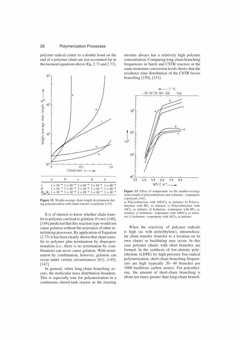
26 Polymerization Processes
polymer radical center to a double bond on theend of a polymer chain are not accounted for inthe moment equations above (Eq. 2.71 and 2.73).
Figure 12. Weight-average chain length development dur-ing polymerization with chain transfer to polymer [147]
It is of interest to know whether chain trans-fer to polymer can lead to gelation. Flory [148],[149] predicted that this reaction type would notcause gelation without the assistance of other in-terlinking processes. By application of Equation(2.73) it has been clearly shown that chain trans-fer to polymer plus termination by dispropor-tionation (i.e., there is no termination by com-bination) can never cause gelation. With termi-nation by combination, however, gelation canoccur under certain circumstances [61], [145],[147].
In general, when long-chain branching oc-curs, the molecular mass distribution broadens.This is especially true for polymerization in acontinuous stirred-tank reactor as the reacting
mixture always has a relatively high polymerconcentration. Comparing long-chain branchingfrequencies in batch and CSTR reactors at thesame monomer conversion levels shows that theresidence time distribution of the CSTR favorsbranching [150], [151].
Figure 13. Effect of temperature on the number-averagechain length of polyisobutylene and isobutene – isopropenecopolymer [161]a) Polyisobutylene with AlEtCl2 as initiator; b) Polyiso-butylene with BF3 as initiator; c) Polyisobutylene withAlCl3 as initiator; d) Isobutene – isopropene with BF3 asinitiator; e) Isobutene – isopropene with AlEtCl2 as initia-tor; f) Isobutene – isopropene with AlCl3 as initiator
When the reactivity of polymer radicalsis high (as with polyethylene), intramolecu-lar chain transfer (transfer to a location on itsown chain) or backbiting may occur. In thiscase polymer chains with short branches areformed. In the synthesis of low-density poly-ethylene (LDPE) by high-pressure free-radicalpolymerization, short-chain branching frequen-cies are high (typically 20 – 40 branches per1000 backbone carbon atoms). For polyethyl-ene, the amount of short-chain branching isabout ten times greater than long-chain branch-

Polymerization Processes 27
ing. For polyethylene the backbiting reactioncan be represented as follows
with n = 3 and 4 most probable [152].
Reactions with Double Bonds in PolymerChains. When a radical center on the end ofa polymer chain adds to a double bond on theend of a polymer chain, a tri-branching point isformed.
Terminal double bonds on the ends of poly-mer chains may be formed by chain transferto monomer, termination by disproportionation,and by β-scission at backbone radical centers.
Reaction with double bonds located on thepolymer backbone (internal or pendant doublebonds) leads to formation of tetra-branchingcenters.
Pendant double bonds are obtained whenmonomers containing two or more reactive dou-ble bonds are polymerized. For example, thehomopolymerization of a diene and the co-polymerization of vinyl and divinyl monomersproduces polymer chains with pendant doublebonds. The photopolymerization of multifunc-tional monomers is used in surface coatings andin the replication of optical discs [153–155]. Fordensely cross-linked systems the buildup of rad-ical concentration is so rapid that the stationary-state hypothesis may not be valid. Superab-sorbent polymers used in diapers and porous or-
ganic packagings used in size exclusion chro-matography are lightly cross-linked polymericnetworks. The kinetics of copolymerization ofvinyl and divinyl monomers are discussed inmore detail in Section 2.3.3.
2.2.2. Ionic Polymerization
The energy required to form a pair of ions froma neutral molecule is large, and therefore thesevery unstable ions must be stabilized by sol-vation at low temperature before polymeriza-tion will occur. Polar solvents cannot be usedto solvate ions because they are overly reactiveand destroy the ionic initiators. Ionic polymer-izations are usually carried out at low tempera-ture in solvents of low polarity. These solventsmay give ion pairs as well as free ions. Thus,a propagating ionic chain may have a counter-ion close to the active center during its growth.The proximity of the ion on the growing chainto its counterion depends on the type of coun-terion, which is determined by the initiator type,and the solvation power of the solvent. There-fore, unlike free-radical polymerization the typeof initiator and the nature of the solvent have alarge effect on monomer addition during chaingrowth. The propagation rate constant, there-fore, depends not only on temperature but alsoon the type of initiator and the type and amountof solvent.
For ionic chain-growth polymerizations insolvents with high solvating power where thedistance between the propagating active cen-ter and the counterion is large, the factors gov-erning the stereochemistry are similar to thosefor free-radical polymerization. However, in sol-vents with poor solvating power, there may beextensive coordination between initiator, propa-gating chain end, and monomer, which results inisotactic (or syndiotactic) placements almost ex-clusively, i.e., stereospecific polymerization oc-curs.
Unlike radical polymerization, bimoleculartermination between active centers does not oc-cur in ionic polymerization. Termination of anactive center on a polymer chain occurs by reac-tion with the counterion, solvent, monomer, orother species. Often, the initiation reactions arevery fast, and the initiator is consumed in the
28 Polymerization Processes
early stages of polymerization before the poly-mer chains have grown much beyond oligomericsize. In the absence of unimolecular termina-tion a population of polymer chains having thesame molecular mass can grow. The concentra-tion of ionic reactive centers is usually muchlarger than that of radical centers. Ionic poly-merization kinetics are not as well understoodas those radical-based polymerizations becauseof the requirements of extreme purity for thecomponents of the reacting mixture.
Elastomers such as butyl rubber and poly-isoprene; high-density polyethylene; polypro-pylene and its copolymers are widely producedby ionic polymerization. Polypropylene of highmolecular mass cannot be produced by radicalpolymerization. In addition to carbon – carbondouble bonds, carbonyl double bonds [81], [82],alkynes [156], and carbon – nitrogen doublebonds [157] can be polymerized via ionic mech-anisms. However, the discussion here is limitedto carbon – carbon double bonds.
2.2.2.1. Cationic Polymerization
Cationic polymerization proceeds through at-tack on the monomer by an electrophilic species,resulting in heterolytic splitting of the doublebond to produce a carbenium ion [158], [159].
The most important commercial high poly-mers produced by cationic polymerization arepolyisobutylenes and butyl rubber (a copoly-mer of isobutylene and a 1,3-diene, usually iso-prene). A typical polymerization is carried outat about − 100 ◦C in chlorinated solvents suchas chloromethane and is initiated by AlCl3. Thepolymerization is very fast.
In the following section, interesting featuresof cationic polymerization are discussed, but noattempt is made to develop quantitative rate ex-pressions. Carbenium ions are very sensitive to
polar impurities and this often precludes the es-tablishment of a stationary state. It is also diffi-cult to establish what proportion of the initiatorproduces growing polymer chains.
Cationic polymerization of vinyl monomersis essentially limited to those with electron-donating substituents such as 1,1-dialkyl,alkoxy, phenyl or vinyl groups. Cationic poly-merization involves initiation, propagation, ter-mination, and chain transfer to small moleculesmuch as in free-radical polymerization.
To initiate cationic polymerization, protonicacids such as H2SO4, HClO4, and H3PO4 orLewis acids such as BF3, AlCl3, TiCl4, andSnCl4 are used. Lewis acids are by far the mostimportant initiators for industrial cationic poly-merizations. Initiation with Lewis acids requiresthe presence of a trace of proton donor such aswater, alcohol, and organic acid or a cation donorsuch as alkyl halide.
In general,
Most polymerizations exhibit a maximumrate at some ratio of initiator and coinitiator con-centrations. This optimum ratio varies widelyfrom one initiator system to another and in someinstances the solvent has an effect on the ratio.(Note that it has also been proposed that the pro-togen or catinogen be referred to as the initiator,and the Lewis acid as coinitiator [159], althoughconventional terminology is exactly the reverse.)
The propagation reaction involves the succes-sive insertion of monomers into the partial bondbetween the propagating species and its coun-terion.
Polymerization Processes 29
The apparent propagation rate constant Kp
depends on the type of initiator and solvent used.In general, Kp becomes larger as the acidity ofthe initiator and/or the dielectric constant of thesolvent increases. This is due to the fact that thereactivity of free ions in monomer addition ismuch greater than that of ion pairs.
A wide variety of reactions may lead to ter-mination of chain growth in cationic polymer-ization, but it is usually ambiguous and difficultto distinguish termination reactions from chain-transfer reactions. Chain transfer to monomer ismost often responsible for the formation of deadpolymer:
If the counterion is sufficiently nucleophilic,termination by combination may occur:
However, this reaction is not very common.In fact, true termination in which the activity ofa chain carrier is lost without regeneration ofan active center is very rare if no impurities ca-pable of destroying an active center are present.However, since the carbenium ion is highly reac-tive, it would be a formidable task to remove allthese impurities from the reaction components.Under commercial conditions it is likely that ac-tive centers are consumed to a significant extentby impurities. Termination reactions in cationicpolymerizations are unimolecular, as they arein anionic and in anionic-coordination polymer-ization. Generally, for cationic systems the poly-merization rate is given by
Rp =K [M]1−3 [I] (2.85)
The first-order rate with respect to initiator con-centration is a consequence of the fact that ter-mination reactions are unimolecular. The overallactivation energy for polymerization ER may beca.− 40 to 60 kJ/mol [160]. For many polymer-ization systems ER is negative and the rather un-usual phenomenon of increasing polymerizationrate with decreasing temperature is observed.The activation energy for the degree of poly-merization is always negative, and therefore theaverage chain length decreases with increasingtemperature. Usually, cationic polymerizations
can produce polymer with sufficient molecularmass only at very low temperatures. Figure 13shows the Arrhenius plot for the number-averagechain length [161]. There is a change in the slopeof this plot around − 100 ◦C. This has been at-tributed to a change in the chain termination stepfrom chain transfer to monomer below− 100 ◦Cto chain transfer to solvent above − 100 ◦C.
Table 1. Effect of counterion on the propagation rate constants (K−p
and K ±p ) in the anionic polymerization of styrene in THF at 25 ◦C
Counterion K ±p K−p K× 107
Li+ 160 6.5× 10⁴ 2.2
Na+ 80 6.5× 10⁴ 1.5
K+ 60 – 80 6.5× 10⁴ 0.8
Rb+ 50 – 80 6.5× 10⁴ 0.1
Cs+ 22 6.5× 10⁴ 0.02
2.2.2.2. Anionic Polymerization
Anionic polymerizations show many of thesame characteristics as cationic polymeriza-tions. However, since the nature of carbanionsis different from carbenium ions, there are dis-tinct differences. In contrast to cationic poly-merization, neither termination nor chain trans-fer occur in many anionic polymerizations (liv-ing polymerization) especially when polar sub-stances are absent. Anionic active centers areusually much more stable than cationic activecenters. Although anionic polymerizations pro-ceed rapidly at low temperatures, they are notusually as temperature sensitive as cationic poly-merizations, and polymerizations usually pro-ceed well at ambient temperature and higher.
A variety of basic initiators have been usedto initiate anionic polymerizations [162], [163].The initiation involves the addition of an anion(base) to the double bond of the monomer.
where the C− · · ·G+ bond can have characterranging from partially covalent to completelyionic. Alkyllithium initiators have been mostwidely used in the polymerization of butadieneand isoprene, since they are easy to prepare andare soluble in hydrocarbon solvents. A compli-cation which arises when alkyllithiums are used

30 Polymerization Processes
in nonpolar solvents such as benzene, toluene,cyclohexane, and n-hexane is association of var-ious organolithium species. This phenomenonis important, since the associated species are es-sentially unreactive in propagation [162], [164].
Propagation occurs by the successive inser-tion of monomers into the partial bond betweenthe propagating anion and its cationic counter-ion.
The polymerization rate is fundamentally ex-pressed by Rp = Kp [M] [M−], where [M−] isthe concentration of active species. When non-polar solvents such as dioxane are used, all activespecies may be ion pairs. However, in polar sol-vents such as THF, the effect of dissociation tofree ions on polymerization rate cannot be ne-glected. Therefore, the propagation rate is givenby the sum of the rates for free propagatinganions (R−) and for ion pairs, R−(G+).
Rp =K−p[
R−]
[M] +K±p[
R−(
G+)]
[M] (2.88)
The two propagating species are in equilibrium,
where K is the dissociation constant and is givenby
K=[
R−] [
G+]
/[
R−(
G+)]
(2.90)
Some experimental values for K±p and K−pare listed in Table 1 [165], [166]. Considerthe simple example of the anionic polymeriza-tion of styrene in THF at 25 ◦C, initiated bysodium naphthalide with an initial concentration[I] = 1× 10⁻³ mol/L. Assuming the initiationreaction is instantaneous, [R−] = 1.22× 10⁻⁵
and [R− (G+)] = 9.88 × 10⁻⁴mol/L. There-fore,
K−p[
R−]
[M]
K±p [R− (G+)] [M]=
(
6.5 × 10⁴) (
1.22 × 10⁻⁵)
(80)(
9.88 × 10⁻⁴)
= 10.0 (2.91)
As shown here, although the concentration offree ions is only 1.2 % of the total propagatingspecies, approximately 90 % of the monomer isconsumed by the free ion.
Since carbanions are relatively stable, anionicpolymerization with carefully purified reagentsmay lead to systems in which chain terminationis absent. Such polymers are referred to as livingpolymers [167], [168].
Let us now develop an expression for thechain length distribution for living polymer. As-suming that initiation is instantaneous, the to-tal number of growing chains N I is constantthroughout the polymerization. Now a monomermolecule adds to a polymer chain as shown inFigure 14. The probability that it adds to poly-mer chain (1) is 1/N I, and that it does not add topolymer chain (1) is 1− 1/N I. Therefore, whenNM monomer units have been consumed andbound into polymer chains the probability thata randomly selected polymer chain possesses r
monomer units is given by a binomial distribu-tion:
N (r) =
(
NM
r
){
1
NI
}r {
1−1
NI
}NM−r
(2.92)
N (r) is also the number chain length distribu-tion. Since 1/N I≪ 1 and r is large, the binomialdistribution reduces to the Poisson distribution:
N (r) =e−ηηr
r!(2.93)
where η = NM/N I, which is equal to the number-average chain length, PN.
Figure 14. Schematic drawing for the derivation of chainlength distribution in living polymerization
The weight chain length distribution W (r)and the weight-average chain length PW aregiven by
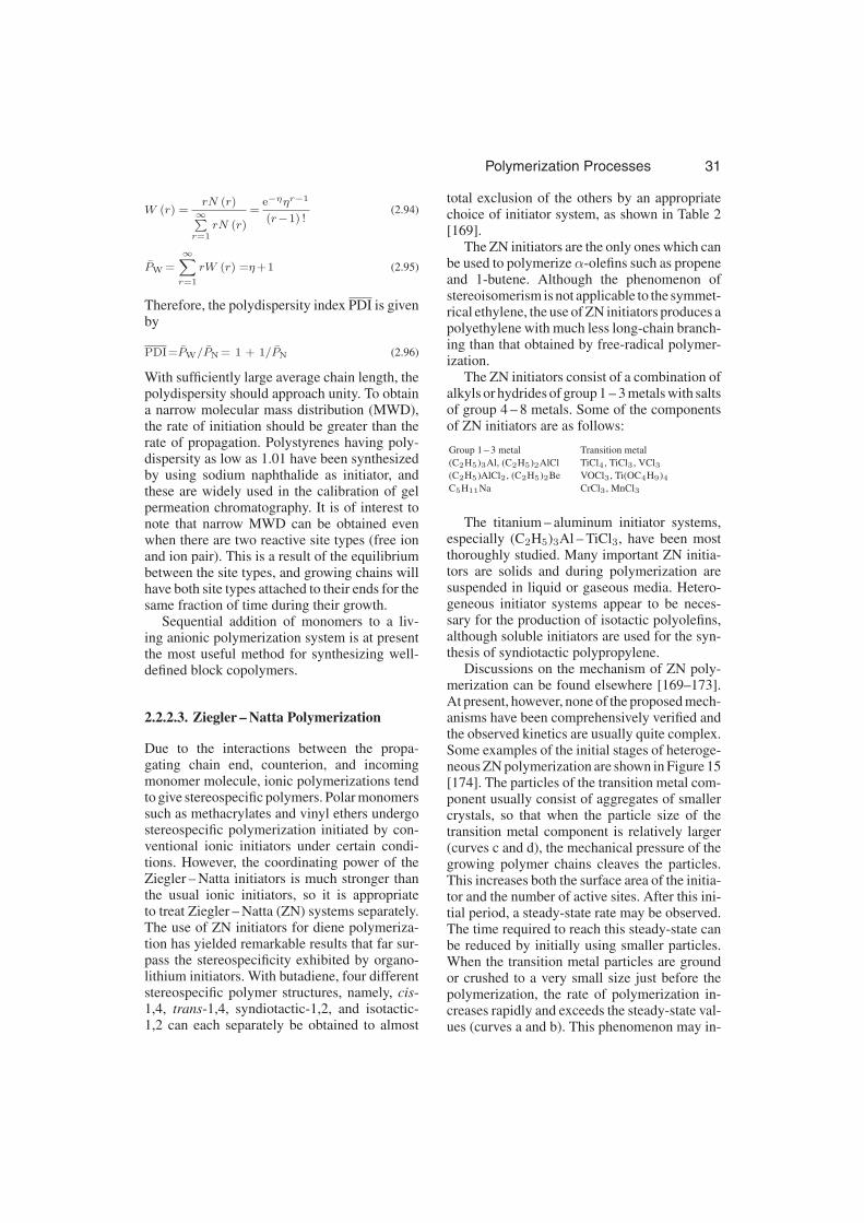
Polymerization Processes 31
W (r) =rN (r)∞∑
r=1rN (r)
=e−ηηr−1
(r−1) !(2.94)
PW =∞∑
r=1
rW (r) =η+1 (2.95)
Therefore, the polydispersity index PDI is givenby
PDI=PW/PN = 1 + 1/PN (2.96)
With sufficiently large average chain length, thepolydispersity should approach unity. To obtaina narrow molecular mass distribution (MWD),the rate of initiation should be greater than therate of propagation. Polystyrenes having poly-dispersity as low as 1.01 have been synthesizedby using sodium naphthalide as initiator, andthese are widely used in the calibration of gelpermeation chromatography. It is of interest tonote that narrow MWD can be obtained evenwhen there are two reactive site types (free ionand ion pair). This is a result of the equilibriumbetween the site types, and growing chains willhave both site types attached to their ends for thesame fraction of time during their growth.
Sequential addition of monomers to a liv-ing anionic polymerization system is at presentthe most useful method for synthesizing well-defined block copolymers.
2.2.2.3. Ziegler – Natta Polymerization
Due to the interactions between the propa-gating chain end, counterion, and incomingmonomer molecule, ionic polymerizations tendto give stereospecific polymers. Polar monomerssuch as methacrylates and vinyl ethers undergostereospecific polymerization initiated by con-ventional ionic initiators under certain condi-tions. However, the coordinating power of theZiegler – Natta initiators is much stronger thanthe usual ionic initiators, so it is appropriateto treat Ziegler – Natta (ZN) systems separately.The use of ZN initiators for diene polymeriza-tion has yielded remarkable results that far sur-pass the stereospecificity exhibited by organo-lithium initiators. With butadiene, four differentstereospecific polymer structures, namely, cis-1,4, trans-1,4, syndiotactic-1,2, and isotactic-1,2 can each separately be obtained to almost
total exclusion of the others by an appropriatechoice of initiator system, as shown in Table 2[169].
The ZN initiators are the only ones which canbe used to polymerize α-olefins such as propeneand 1-butene. Although the phenomenon ofstereoisomerism is not applicable to the symmet-rical ethylene, the use of ZN initiators produces apolyethylene with much less long-chain branch-ing than that obtained by free-radical polymer-ization.
The ZN initiators consist of a combination ofalkyls or hydrides of group 1 – 3 metals with saltsof group 4 – 8 metals. Some of the componentsof ZN initiators are as follows:
Group 1 – 3 metal Transition metal
(C2H5)3Al, (C2H5)2AlCl TiCl4, TiCl3, VCl3(C2H5)AlCl2, (C2H5)2Be VOCl3, Ti(OC4H9)4C5H11Na CrCl3, MnCl3
The titanium – aluminum initiator systems,especially (C2H5)3Al – TiCl3, have been mostthoroughly studied. Many important ZN initia-tors are solids and during polymerization aresuspended in liquid or gaseous media. Hetero-geneous initiator systems appear to be neces-sary for the production of isotactic polyolefins,although soluble initiators are used for the syn-thesis of syndiotactic polypropylene.
Discussions on the mechanism of ZN poly-merization can be found elsewhere [169–173].At present, however, none of the proposed mech-anisms have been comprehensively verified andthe observed kinetics are usually quite complex.Some examples of the initial stages of heteroge-neous ZN polymerization are shown in Figure 15[174]. The particles of the transition metal com-ponent usually consist of aggregates of smallercrystals, so that when the particle size of thetransition metal component is relatively larger(curves c and d), the mechanical pressure of thegrowing polymer chains cleaves the particles.This increases both the surface area of the initia-tor and the number of active sites. After this ini-tial period, a steady-state rate may be observed.The time required to reach this steady-state canbe reduced by initially using smaller particles.When the transition metal particles are groundor crushed to a very small size just before thepolymerization, the rate of polymerization in-creases rapidly and exceeds the steady-state val-ues (curves a and b). This phenomenon may in-

32 Polymerization Processes
Table 2. Stereospecific polymerization of butadiene [169]
dicate the existence of highly active but short-lived sites. This kind of behavior can be avoidedby aging the initiator system prior to addition ofmonomer.
Figure 15. Effect of previous physical treatment on a sampleof α–TiCl3 on the propene polymerization rate (in gramsC3H6 per gram TiCl3 per hour) at constant pressure andtemperaturea), b) Ground α–TiCl3 (sizes≤ 2 µm); c), d) Unground α–TiCl3 (sizes 1 – 10 µm)
Many ZN polymerizations exhibit a contin-uous decrease in rate rather than reaching asteady-state in which the rate curve reaches amaximum and then continues to decline. Therate of decline varies with the polymerizationsystem used. The decline in polymerization ratehas been attributed to (1) a decrease in the num-ber of active centers, (2) a lowering of activ-ity of individual active centers due to structuralchanges, and (3) a lowering of activity of in-dividual active centers due to encapsulation bypolymer.
In this section a very simple example is con-sidered, too approximate to accurately describereal systems, but useful to illustrate a modelbuilding process. Consider the following poly-merization scheme [175].
1) Adsorption of monomer (M) on the activesite
where P∗l is a growing chain with unit chainlength and A is a vacant active site.
2) Propagation
where P∗r is the growing polymer chain withlength r
3) Desorption of polymer chain from the activesite
where Pr is a dead polymer molecule withchain length r.
Assuming that the polymer chain is suffi-ciently long (long-chain assumption), the poly-merization rate Rp is given by
Rp =Kp [P∗] [M] (2.100)
where [P∗] is the total concentration of active
sites, namely, [P ∗] =∞∑
r=1
[P∗r ] .
Polymerization Processes 33
If the stationary-state hypothesis is applied to[P∗],
KA [M] [A] =KD [P∗] (2.101)
Each active site is either occupied by growingpolymer chains or is vacant. Denoting the totalconcentration of adsorption sites by [A]0,
[A]0 = [A] + [P∗] (2.102)
Combining Equations (2.101) and (2.102) gives
[P∗] =K [A]0 [M] / (1+K [M]) (2.103)
where K = KA/KD. Therefore, the polymeriza-tion rate is given by
Rp =KpK [A]0 [M] / (1+K [M]) (2.104)
Next consider the instantaneous molecular massdistribution for this process. The population bal-ance equations for growing polymer chains are
1
V
d(
V[
P∗1])
dt=KA [M] [A]
−Kp [M] [P∗1] −KD [P∗1] (2.105)
1
V
d (V [P∗r ])
dt=Kp [M]
[
P∗r−1
]
−Kp [M] [P∗r ]
−KD [P∗r ] (r≥2) (2.106)
By application of the SSH for [P∗r ],
[P∗l ] =1
1+τ ′[A] (2.107)
[P ∗r ] =1
1+τ ′
[
P∗r−1
]
(2.108)
where τ ′ = KD/(Kp [M]). Therefore,
[Pr] =KD [P∗r ] =KD [A](
Φ′)r
(2.109)
where Φ′ = 1/(1 + τ ′).The number and weight chain length distri-
butions are given by
N (r) =[Pr]∞∑
r=1[Pr]
=(
1−Φ′) (
Φ′)r−1
(2.110)
W (r) =r [Pr]∞∑
r=1r [Pr]
=r(
1−Φ′)2 (
Φ′)r−1
(2.111)
where Φ′ is the probability that a growing poly-mer chain adds another monomer molecule, and
(1−Φ′) is the probability that a growing chainstops growing.
Therefore, Equations (2.110) and (2.111) areessentially the same as Equations (2.8) and (2.9)or Equation (2.56). The polydispersity index(PDI) for instantaneously formed polymer istwo.
An interesting feature of heterogeneous ZNinitiators is the very broad MWD of the polymersproduced, although the above simple model pre-dicts PDI = 2 for instantaneously formed poly-mer. The PDI of accumulated polymer may be10 or higher. In the case of copolymerization, thecompositional heterogeneity is also large evenwhen monomer ratios are kept constant duringpolymerization. Presently, there are two maintheories which try to explain these large disper-sities, namely, the presence of a distribution ofactivities for the active sites or diffusional ef-fects which limit the transport of reactants to theactive sites [176].
2.3. Copolymerization
Copolymerization permits the synthesis of an al-most unlimited number of polymer types and istherefore often used to obtain a better balance ofproperties for commercial applications. Copoly-mers may be synthesized by chain-growthand step-growth polymerization. In step-growthpolymerization, different monomers with thesame type of functional group generally showonly minor differences in reactivity. As a result,most copolymers prepared by step-growth poly-merization contain essentially random place-ments of repeat units, with the composition ofthe copolymers essentially the same as those ofthe original monomer mixture.
In contrast, strong selective effects often oc-cur in chain-growth copolymerizations, and thecomposition of the copolymer formed may dif-fer greatly from the composition of the origi-nal monomer mixture. This section deals ex-clusively with chain-growth copolymerization.Chain-growth copolymerization can be carriedout with various types of active centers includingfree-radical, cationic, and anionic species. Free-radical copolymerization is most commonlyused due to its higher alternating tendencies.
34 Polymerization Processes
2.3.1. Copolymer Composition
The composition of copolymers cannot be de-termined from a knowledge of the homopoly-merization rates of each monomer. In 1944,the instantaneous copolymer composition equa-tion was proposed independently by several re-searchers by assuming that the chemical activityof a propagating chain depends solely on the ter-minal monomer unit on which the active centeris located [177–180]. This model is called theterminal model, and the copolymer chain canbe considered as a first-order Markov chain. Forbinary systems, the following four propagationreactions are possible.
where P∗m,n,1 is a live copolymer chain with m
units of monomer 1 (M1) and n units of monomer2 (M2) bound in the polymer chain and with theactive center located on terminal monomer unit1.
The reactivity of the propagating species maybe affected by the penultimate monomer unit. Insuch cases, the model is referred to as the penul-timate model or a second-order Markov chain[181], [182] and propagation consists of eightreactions. Further expansion is possible by con-sidering the effects of remote units preceding thepenultimate unit, such as the pen-penultimatemodel [183–185].
It is customarily assumed that the propa-gation rate constants are independent of chainlength and that the chains are sufficiently large( long-chain assumption, LCA). The LCA in-cludes the approximation that monomer con-sumed in reactions other than propagation is neg-ligible and that the SSH is valid for each typeof active center; i.e., the rate of formation ofany type of active center is equal to its rate ofconsumption. Statistically, these conditions areequivalent to the statistical stationary condition[185–187].
Now consider a binary copolymerizationwhose propagation reactions follow the termi-
nal model. The specific polymerization rates ofmonomers 1 and 2 are given by
−1
V
d (V [M1])
dt=K11 [P∗1] [M1] +K21 [P∗2] [M1]
(2.116)
−1
V
d (V [M2])
dt=K12 [P∗1] [M2] +K22 [P∗2] [M2]
(2.117)
where [P∗1] and [P∗2] are the total concentrationsof active centers of types 1 and 2 with
[P∗1] =
∞∑
m=1
∞∑
n=1
[
P∗m,n,1
]
(2.118)
[P∗2] =
∞∑
m=1
∞∑
n=1
[
P∗m,n,2
]
(2.119)
Application of the SSH gives
K21 [P∗2] [M1] =K12 [P∗1] [M2] (2.120)
Dividing Equation (2.116) by Equation (2.117)and using Equation (2.120) gives the instanta-neous copolymer composition equation:
F1
F2=−d (V [M1])
−d (V [M2])=
[M1] (r1 [M1] + [M2])
[M2] ([M1] +r2 [M2])
(2.121a)
or
F1 =r1f 2
1 +f1 f2
r1f 21 +2f1f2 +r2f 2
2
(2.121b)
where F1 and F2 are the mole fractions ofmonomers 1 and 2 in the copolymer producedinstantaneously, and f 1 and f 2 are the mole frac-tions of unreacted monomer. The reactivity ra-tios are defined by
r1 =K11
K12(2.122)
r2 =K22
K21(2.123)
It is straightforward to extend this methodto multicomponent polymerization [188–190].Note that Equation (2.121 a or b) is strictly validonly for infinitely long polymer chains and itsapplication to short chains may introduce sig-nificant error [191–193].
When applying Equation (2.121 a or b), it isusually assumed that all of the copolymer chains
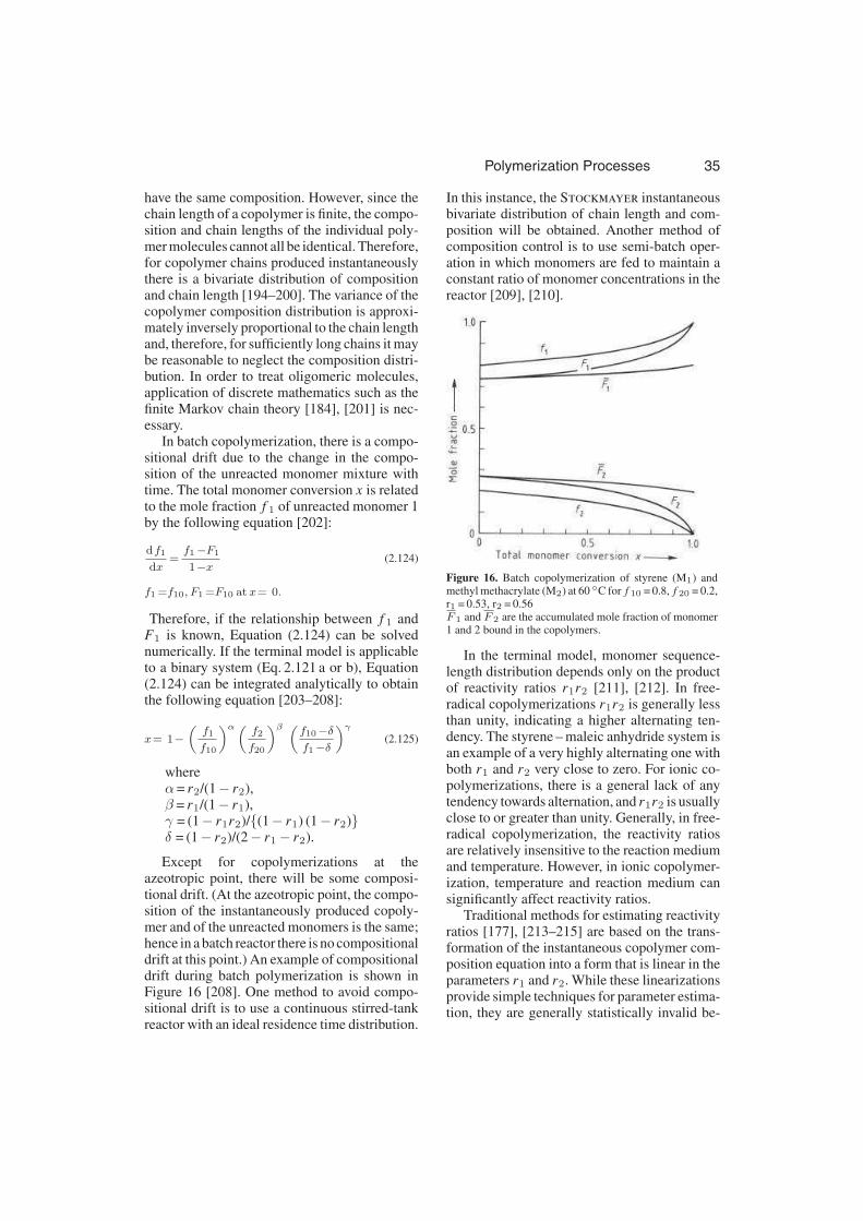
Polymerization Processes 35
have the same composition. However, since thechain length of a copolymer is finite, the compo-sition and chain lengths of the individual poly-mer molecules cannot all be identical. Therefore,for copolymer chains produced instantaneouslythere is a bivariate distribution of compositionand chain length [194–200]. The variance of thecopolymer composition distribution is approxi-mately inversely proportional to the chain lengthand, therefore, for sufficiently long chains it maybe reasonable to neglect the composition distri-bution. In order to treat oligomeric molecules,application of discrete mathematics such as thefinite Markov chain theory [184], [201] is nec-essary.
In batch copolymerization, there is a compo-sitional drift due to the change in the compo-sition of the unreacted monomer mixture withtime. The total monomer conversion x is relatedto the mole fraction f 1 of unreacted monomer 1by the following equation [202]:
df1
dx=f1−F1
1−x(2.124)
f1 =f10, F1 =F10 at x= 0.
Therefore, if the relationship between f 1 andF1 is known, Equation (2.124) can be solvednumerically. If the terminal model is applicableto a binary system (Eq. 2.121 a or b), Equation(2.124) can be integrated analytically to obtainthe following equation [203–208]:
x= 1−
(
f1
f10
)α (
f2
f20
)β (
f10−δ
f1−δ
)γ
(2.125)
whereα = r2/(1− r2),β = r1/(1− r1),γ = (1− r1r2)/{(1− r1) (1− r2)}δ = (1− r2)/(2− r1− r2).
Except for copolymerizations at theazeotropic point, there will be some composi-tional drift. (At the azeotropic point, the compo-sition of the instantaneously produced copoly-mer and of the unreacted monomers is the same;hence in a batch reactor there is no compositionaldrift at this point.) An example of compositionaldrift during batch polymerization is shown inFigure 16 [208]. One method to avoid compo-sitional drift is to use a continuous stirred-tankreactor with an ideal residence time distribution.
In this instance, the Stockmayer instantaneousbivariate distribution of chain length and com-position will be obtained. Another method ofcomposition control is to use semi-batch oper-ation in which monomers are fed to maintain aconstant ratio of monomer concentrations in thereactor [209], [210].
Figure 16. Batch copolymerization of styrene (M1) andmethyl methacrylate (M2) at 60 ◦C for f 10 = 0.8, f 20 = 0.2,r1 = 0.53, r2 = 0.56F 1 and F 2 are the accumulated mole fraction of monomer1 and 2 bound in the copolymers.
In the terminal model, monomer sequence-length distribution depends only on the productof reactivity ratios r1r2 [211], [212]. In free-radical copolymerizations r1r2 is generally lessthan unity, indicating a higher alternating ten-dency. The styrene – maleic anhydride system isan example of a very highly alternating one withboth r1 and r2 very close to zero. For ionic co-polymerizations, there is a general lack of anytendency towards alternation, and r1r2 is usuallyclose to or greater than unity. Generally, in free-radical copolymerization, the reactivity ratiosare relatively insensitive to the reaction mediumand temperature. However, in ionic copolymer-ization, temperature and reaction medium cansignificantly affect reactivity ratios.
Traditional methods for estimating reactivityratios [177], [213–215] are based on the trans-formation of the instantaneous copolymer com-position equation into a form that is linear in theparameters r1 and r2. While these linearizationsprovide simple techniques for parameter estima-tion, they are generally statistically invalid be-

36 Polymerization Processes
cause the independent variable has experimentalerror and the dependent variable does not have aconstant variance [216–223]. Both of the latterassumptions are necessary for the linear leastsquares method to be a statistically valid es-timation method. Although it has been shownthat proper experimental design can allow theuse of linear least squares analysis [222], [224],the estimation of the reactivity ratios is a typicalexample of a problem in nonlinear estimation.Reactivity ratios are now generally estimatedby application of procedures based on the sta-tistically valid error-in-variables-model (EVM)[220], [221], [225–230]. These methods allowall the sources of experimental error to be ac-counted for.
In spite of the fact that reactivity ratios ob-tained using invalid estimation procedures haveoften been used, the copolymer compositionequation based on the terminal model has givenuseful predictions. It is generally ineffective touse the copolymer composition equation forcomparing models. Information on the copoly-mer microstructure (e.g., monomer sequencelength distribution) is needed to compare the va-lidity of terminal and penultimate models [179],[231], [232]. Advancements in NMR techniqueshave provided suitable information on sequencelength distribution. However, cases have beenreported in which sequence length distributioninformation does not permit model discrimina-tion [233].
As will be discussed in Section 2.3.2 the com-position equation includes the rate constants ofelementary reactions only in ratios, while therate equation is dependent on their absolute val-ues, and therefore success of the former equationdoes not insure success of the latter [234].
2.3.2. Kinetics of Copolymerization
Consider the kinetics of free-radical copolymer-ization of monomers M1 and M2, assuming theterminal model is applicable. Important elemen-tary reactions are:
Initiation
Propagation
Transfer to monomer
Transfer to small molecule
Termination by disproportionation
Termination by combination
where R•
m, n, 1 is a polymer radical with m unitsof monomer 1 (M1) and n units of monomer 2(M2) bound in the polymer chain with activecenter located on monomer unit 1. Pm ,n is apolymer molecule with m units of monomer 1and n units of monomer 2. The polymerizationrate, Rp is given by
Rp =K11 [R·
1] [M1] +K12 [R·
1] [M2]
+K21 [R·
2] [M1] +K22 [R·
2] [M2]
=Kp [R·] [M] (2.126)
where [R•
1] and [R•
2] are given byEquations (2.118) and (2.119) and[R·] = [R·
1] + [R·
2] , [M] = [M1] + [M2] , andKp is defined by
Kp = (K11f1 +K12f2)ϕ·
1 + (K21f1 +K22f2)ϕ·
2
(2.127)

Polymerization Processes 37
where f 1 = [M1]/[M], and ϕ•
1 = [R•
1]/[R•
].Equation (2.127) is an example of a pseudo-
kinetic rate constant [145–147], [209], [210],[235–238]. For an N-component system, thepseudo-kinetic rate constants can be defined asfollowsPropagation
Kp =N∑
i=1j=1
Kij ϕ·
i fj (2.128)
Chain transfer to monomer
Kfm =N∑
i=1j=1
Kfijϕ·
i fj (2.129)
Chain transfer to small molecule
KfT =N∑
i=1
KfTiϕ·
i (2.130)
Termination by disproportionation
Ktd =
N∑
i=1j=1
Ktdijϕ·
iϕ·
j (2.131)
Termination by combination
Ktc =N∑
i=1j=1
Ktcij ϕ·
iϕ·
j (2.132)
Even though these pseudo-kinetic rate constantsdepend on the monomer mole fraction andchange with time in a batch reactor, the simpli-fication achieved when dealing with multicom-ponent polymerizations is very great. Further-more, since the mole fraction of each polymer
radical type ϕ•
i is independent of chain lengthfor sufficiently long chains, these same pseudo-kinetic rate constants can be used to calculatemolecular mass distribution as well as poly-merization rate [61],[235] . Therefore, by us-ing pseudo-kinetic rate constants, a multicompo-nent polymerization reduces to a homopolymer-ization, and therefore Equations (2.55) – (2.64)are all applicable for copolymerization. Withappropriate definitions for pseudo-kinetic rateconstants, this method may also be usefully ap-plied when copolymerization kinetics follow thepenultimate model [235].
In the early development of the kinetics ofcopolymerization, chemically controlled bimo-lecular termination was assumed to be operable[239–241]. However, since these reactions havebeen shown to be diffusion controlled [120–122], [242], Equations (2.131) and (2.132) mustbe modified by using appropriate models whichaccount for this. In this context, the use of thecross-termination factor, ϕ= Kt12/(K11K12)0.5,is not acceptable. Several models for diffusion-controlled termination of binary copolymeriza-tion have been proposed. Atherton and North
[243], [244] proposed the following for the ter-mination constant.
Kt =Kt11F1 +Kt22F2 (2.133)
The mole fractions of monomers bound in poly-mer chains F1 and F2 can be calculated by us-ing the copolymer composition equation. On theother hand, Russo and Munari [245] proposedthe use of penultimate effect for the terminationreactions since segmental diffusion is highly de-pendent on the last two portions of the chain.
Until the mid 1980s, a prevailing view of co-polymerization kinetics was that the propagationprocess is, in most cases, correctly described bythe terminal model, whereas the termination pro-cess involves complexity still to be elucidated.However, it has also been speculated that it is thepropagation step that needs further study, whilethe termination step is well described by simplemodels such as Equation (2.133), and the penul-timate effect on propagation reactions is beingexamined from the point of view of copolymer-ization rates [233], [246–252].
2.3.3. Copolymerization of Vinyl andDivinyl Monomers
The use of the terms vinyl and divinyl here isnot according to their strict definitions. Here, avinyl monomer is defined as a monomer witha single reactive double bond (a double bondwhich will readily add to a radical center) and adivinyl monomer is a monomer which has twosuch double bonds.
The free-radical copolymerization of vinyland divinyl monomers is important in the manu-facture of ion-exchange resins, chromatographicpackings, superabsorbent polymers (with arapidly growing market in baby diapers and
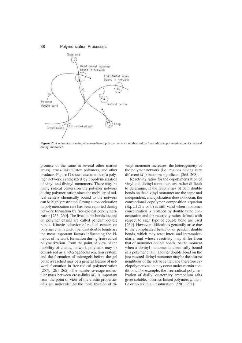
38 Polymerization Processes
Figure 17. A schematic drawing of a cross-linked polymer network synthesized by free-radical copolymerization of vinyl anddivinyl monomer
promise of the same in several other marketareas), cross-linked latex polymers, and otherproducts. Figure 17 shows a schematic of a poly-mer network synthesized by copolymerizationof vinyl and divinyl monomers. There may bemany radical centers on the polymer networkduring polymerization since the mobility of rad-ical centers chemically bound to the networkcan be highly restricted. Strong autoaccelerationin polymerization rate has been reported duringnetwork formation by free-radical copolymeri-zation [253–260]. The live double bonds locatedon polymer chains are called pendant doublebonds. Kinetic behavior of radical centers onpolymer chains and of pendant double bonds arethe most important factors influencing the ki-netics of network formation during free-radicalpolymerization. From the point of view of themobility of chains, network polymers may beconsidered as a heterogeneous reaction system,and the formation of microgels before the gelpoint is reached may be a general feature of net-work formation in free-radical polymerization[257], [261–265]. The number-average molec-ular mass between cross-links Mc is importantfrom the point of view of the elastic propertiesof a gel molecule. As the mole fraction of di-
vinyl monomer increases, the heterogeneity ofthe polymer network (i.e., regions having verydifferent Mc) becomes significant [265–268].
Reactivity ratios for the copolymerization ofvinyl and divinyl monomers are rather difficultto determine. If the reactivities of both doublebonds on the divinyl monomer are the same andindependent, and cyclization does not occur, theconventional copolymer composition equation(Eq. 2.121 a or b) is still valid when monomerconcentration is replaced by double bond con-centration and the reactivity ratios defined withrespect to each type of double bond are used[269]. However, difficulties generally arise dueto the complicated behavior of pendant doublebonds, which may react inter- and intramolec-ularly, and whose reactivity may differ fromthat of monomer double bonds. At the momentwhen a divinyl monomer is chemically boundin a polymer chain, another double bond on thejust-reacted divinyl monomer may be the nearestneighbour of the active center, and therefore cy-clopolymerization may occur under certain con-ditions. For example, the free-radical polymer-ization of diallyl quaternary ammonium saltsgives soluble, not cross-linked polymers with lit-tle or no residual unsaturation [270], [271].
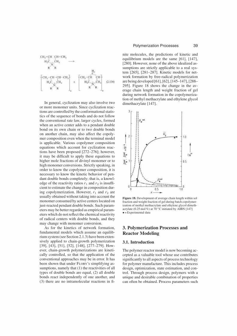
Polymerization Processes 39
In general, cyclization may also involve twoor more monomer units. Since cyclization reac-tions are controlled by the conformational statis-tics of the sequence of bonds and do not followthe conventional rate law, larger cycles, formedwhen an active center adds to a pendant doublebond on its own chain or to two double bondson another chain, may also affect the copoly-mer composition even when the terminal modelis applicable. Various copolymer compositionequations which account for cyclization reac-tions have been proposed [272–276]; however,it may be difficult to apply these equations tohigher mole fractions of divinyl monomer or tohigh monomer conversions. Strictly speaking, inorder to know the copolymer composition, it isnecessary to know the kinetic behavior of pen-dant double bonds completely; that is, a knowl-edge of the reactivity ratios r1 and r2 is insuffi-cient to estimate the change in composition dur-ing copolymerization. However, r1 and r2 areusually obtained without taking into account themonomer consumed by active centers located onjust-reacted pendant double bonds. Such param-eters may be better regarded as empirical param-eters which do not reflect the chemical reactivityof radical centers with double bonds, and theymay change with monomer conversion.
As for the kinetics of network formation,fundamental models which assume an equilib-rium system (see Section 2.1.3) have been exten-sively applied to chain-growth polymerization[39], [43], [51], [52], [148], [277–279]. How-ever, chain-growth polymerizations are kineti-cally controlled, so that the application of theconventional approaches may be in error. It hasbeen shown that under Flory’s simplifying as-sumptions, namely that (1) the reactivities of alltypes of double bonds are equal, (2) all doublebonds react independently of one another, and(3) there are no intramolecular reactions in fi-
nite molecules, the predictions of kinetic andequilibrium models are the same [61], [147],[280]. However, none of the above idealized as-sumptions are strictly applicable to a real sys-tem [265], [281–287]. Kinetic models for net-work formation by free-radical polymerizationare being developed [61], [62], [145–147], [288–295]. Figure 18 shows the change in the av-erage chain length and weight fraction of gelduring network formation in the copolymeriza-tion of methyl methacrylate and ethylene glycoldimethacrylate [147].
Figure 18. Development of average chain length within solfraction and weight fraction of gel during batch copolymer-ization of methyl methacrylate and ethylene glycol dimeth-acrylate (0.25 mol %) at 70 ◦C initiated by AIBN [147]•= Experimental data
3. Polymerization Processes and
Reactor Modeling
3.1. Introduction
The polymer reactor model is now becoming ac-cepted as a valuable tool whose use contributessignificantly to all aspects of process technologyfor polymer manufacture. This includes processdesign, optimization, state estimation, and con-trol. Through process design, polymers with aunique and desirable combination of propertiescan often be obtained. Process parameters such

40 Polymerization Processes
as residence time distribution (RTD) are usuallynot considered by polymer synthesis chemists,although RTD can influence chemical compo-sition distribution (CCD), molecular mass dis-tribution (MWD), long-chain branching (LCD)and gel/sol ratios. In the early days of the poly-mer industry, the chemist played the major rolein product and process development and scale-up. This has changed, with the process engineernow playing a significant role in all phases ofcommercialization of new and improved poly-mer products. His broad experience with pro-cess fundamentals and computer modeling areessential to obtain high-quality products, safelyand economically.
Dynamic reactor models can be used in avariety of ways. Stability and control of poly-mer reactors should be considered at the de-sign stage and control problems minimized then,rather than take corrective action after the plant isbuilt. Complex interactions which are involvedin polymerization (highly nonlinear temperatureand concentration effects) preclude optimal de-sign based on experimentation alone because thecost would be prohibitive. Models can be used toidentify potential sources of product variabilityand strategies to minimize their effects. Modelscan be used to store information on process tech-nology in a concise and readily retrievable andmodifiable form.
Process models can be used to train chemists,chemical engineers, and plant operators and givethem a feel for the dynamics of the polymeriza-tion process.
The most expensive aspect of model devel-opment is experimental estimation of modelparameters; highly instrumented bench-, pilot-scale, and plant-scale reactors are required. Sta-tistically designed experiments should be per-formed to permit efficient parameter estimationand model development. Modeling is an iterativeprocess and the very act of developing a deter-ministic model permits a greater understandingof the relevant microscopic processes which oc-cur during polymerization or polymer modifica-tion. As additional data (plant, pilot-plant, andbench-scale) become available, model structureand parameters can be updated.
This section considers recent developmentsin polymerization/polymer modification pro-cesses and discusses advances in polymer re-actor modeling, state estimation, and control.
3.2. Processes and Reactor Modeling for
Step-Growth Polymerization
3.2.1. Types of Reactors and ReactorModeling
In step-growth polymerization, high molecularmass polymers are usually not produced until thefinal stage of reactions, so that thermal controland mixing of the reaction mixture do not presentserious problems in the earlier stages. However,since the final stage of polymerization is very im-portant for the production of polymers with highmolecular mass, handling of very high viscosi-ties and temperatures and high interfacial areato remove small molecules are required. Variouspolymerization processes and reactor types, bothfor batch and continuous production, have beenproposed. Examples of reactors for high viscosi-ties are shown in Figures 19 and 20. Careful se-lection of the polymerization reactor is very im-portant to produce high-quality polymers [296],[297].
Figure 19. Vertical cone ribbon blade reactor (MitsubishiHeavy Industries)
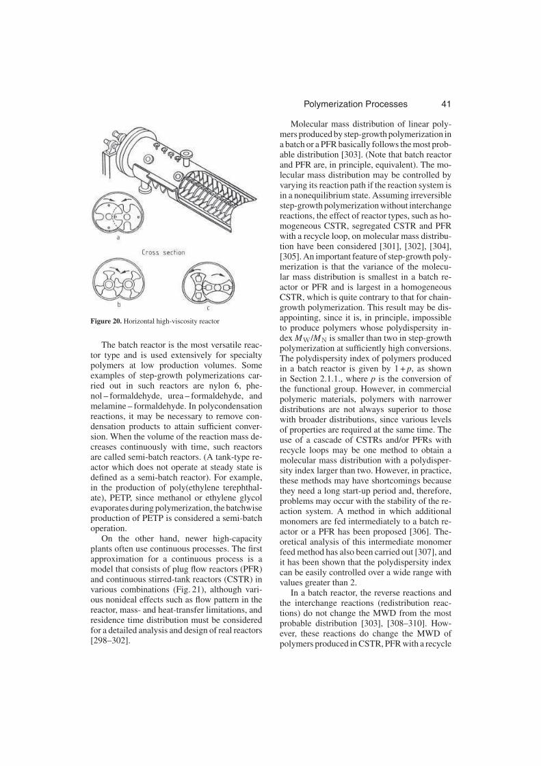
Polymerization Processes 41
Figure 20. Horizontal high-viscosity reactor
The batch reactor is the most versatile reac-tor type and is used extensively for specialtypolymers at low production volumes. Someexamples of step-growth polymerizations car-ried out in such reactors are nylon 6, phe-nol – formaldehyde, urea – formaldehyde, andmelamine – formaldehyde. In polycondensationreactions, it may be necessary to remove con-densation products to attain sufficient conver-sion. When the volume of the reaction mass de-creases continuously with time, such reactorsare called semi-batch reactors. (A tank-type re-actor which does not operate at steady state isdefined as a semi-batch reactor). For example,in the production of poly(ethylene terephthal-ate), PETP, since methanol or ethylene glycolevaporates during polymerization, the batchwiseproduction of PETP is considered a semi-batchoperation.
On the other hand, newer high-capacityplants often use continuous processes. The firstapproximation for a continuous process is amodel that consists of plug flow reactors (PFR)and continuous stirred-tank reactors (CSTR) invarious combinations (Fig. 21), although vari-ous nonideal effects such as flow pattern in thereactor, mass- and heat-transfer limitations, andresidence time distribution must be consideredfor a detailed analysis and design of real reactors[298–302].
Molecular mass distribution of linear poly-mers produced by step-growth polymerization ina batch or a PFR basically follows the most prob-able distribution [303]. (Note that batch reactorand PFR are, in principle, equivalent). The mo-lecular mass distribution may be controlled byvarying its reaction path if the reaction system isin a nonequilibrium state. Assuming irreversiblestep-growth polymerization without interchangereactions, the effect of reactor types, such as ho-mogeneous CSTR, segregated CSTR and PFRwith a recycle loop, on molecular mass distribu-tion have been considered [301], [302], [304],[305]. An important feature of step-growth poly-merization is that the variance of the molecu-lar mass distribution is smallest in a batch re-actor or PFR and is largest in a homogeneousCSTR, which is quite contrary to that for chain-growth polymerization. This result may be dis-appointing, since it is, in principle, impossibleto produce polymers whose polydispersity in-dex MW/MN is smaller than two in step-growthpolymerization at sufficiently high conversions.The polydispersity index of polymers producedin a batch reactor is given by 1 + p, as shownin Section 2.1.1., where p is the conversion ofthe functional group. However, in commercialpolymeric materials, polymers with narrowerdistributions are not always superior to thosewith broader distributions, since various levelsof properties are required at the same time. Theuse of a cascade of CSTRs and/or PFRs withrecycle loops may be one method to obtain amolecular mass distribution with a polydisper-sity index larger than two. However, in practice,these methods may have shortcomings becausethey need a long start-up period and, therefore,problems may occur with the stability of the re-action system. A method in which additionalmonomers are fed intermediately to a batch re-actor or a PFR has been proposed [306]. The-oretical analysis of this intermediate monomerfeed method has also been carried out [307], andit has been shown that the polydispersity indexcan be easily controlled over a wide range withvalues greater than 2.
In a batch reactor, the reverse reactions andthe interchange reactions (redistribution reac-tions) do not change the MWD from the mostprobable distribution [303], [308–310]. How-ever, these reactions do change the MWD ofpolymers produced in CSTR, PFR with a recycle

42 Polymerization Processes
Figure 21. Representative models for polymerization reactorsA) CSTR + PFR; B) CSTR + CSTR + PFR; C) PFRs; D) CSTRs
loop, and intermediate monomer feed method.Some consideration of these reactions in a CSTRis given in [311]. Qualitatively, these effectslower the polydispersity and make the MWDapproach the most probable distribution. Thisresult seems reasonable, since any MWD ap-proaches the most probable distribution witha polydispersity index of two when polymerchains are severed randomly [312], [313].
Other than the common reactor types dis-cussed above, other special types of reactor sys-tem may be applied. For example, in the poly-merization of urethanes, the reaction rates areso high that reaction takes place even when themonomers are being mixed and pumped intomolds. In situ polymerization to form the de-sired articles directly from monomeric liquidsis known as reaction injection molding (RIM)[314], [315]. A schematic of the RIM processis shown in Figure 22. The RIM processing ofpolyesters, epoxy resins, polyamides, and dicy-clopentadienes has also been introduced, al-though more than 95 % of the total produced byRIM is polyurethane [315]. In the RIM process,the reaction is almost complete by the time thematerial fills the mold, and therefore the mix-ing and flow equations must be solved simulta-
neously with those for chemical reactions in arational model for these complex situations.
Figure 22. Schematic drawing of the RIM processa) Monomer A; b) Monomer B; c) Polymerizing mixture;d) Mold; e) Mixer

Polymerization Processes 43
In the finishing stage of nylon 6, nylon 66, andPETP polymerizations, higher molecular masspolymers may be obtained by solid-state poly-merization in which polymerization occurs byheating chips or flakes of a material below itsmelting point in a stream of hot gases in a flu-idized bed or in a drier operated under vacuum[316–320]. The monomer, condensation prod-ucts, and various byproducts diffuse out, andfurther reaction takes place inside the solid. Theprogress of these types of reaction is affectedsignificantly by the diffusion of the condensa-tion products and the morphology of the solid.
Although step-growth polymerization has avery long history, a systematic kinetic treatmentlike that available for free-radical polymeriza-tion does not exist because of limitations due tosystem-specific side reactions and the scarcityof reliable kinetic data. However, this syntheticroute is becoming more important due to thedevelopment of materials synthesized by step-growth polymerization such as aramides, PPS,PEK, and PES. The production technology ofstep-growth polymers seems to have revived asan attractive research area and is enjoying a Re-naissance period.
3.2.2. Specific Processes
Polyamides (see also →Polyamides) aremanufactured by two basic routes. One ofthese is synthesis from cyclic monomers suchas lactams. Polymerization of these substancesrequires ring opening and subsequent chaingrowth. Another class of synthetic polyamidesis formed from diamines and diacids.
The most common types of polyamides arenylon 6 and nylon 66. The term nylon is of-ten used for synthetic aliphatic polyamides. Onenumber indicates that the product was preparedfrom a single monomer and represents the num-ber of carbon atoms in the repeating unit. Twonumbers refer to the number of carbon atoms inthe diamine and that in the diacid, respectively.
Nylon 6 is typically produced by the hy-drolytic polymerization of ε-caprolactam [321–325], although polymers with higher molecularmass can be produced by ionic polymerization[321], [323], [326]. The major reactions in thehydrolytic polymerization are
1) Ring opening of ε-caprolactam by water(Eq. 3.1), which produces aminocaproic acid(ACA)
2) Polycondensation of ACA (Eq. 3.2)3) Acid-catalyzed polyaddition (ring-opening
polymerization) by nucleophilic attack of theamine nitrogen on the lactam (Eq. 3.3)
Step-growth polymerization of the aminoacid (Eq. 3.2) accounts for only a few percentof total polymerization of ε-caprolactam. How-ever, step-growth polymerization is importantsince it usually determines the final degree ofpolymerization at equilibrium. The molecularmass distribution is essentially the most prob-able distribution, except for the presence ofmonomer and cyclic oligomers. Since low mo-lecular mass substances lower the polymer qual-ity, they are usually removed by leaching or vac-uum treatment of the polymer melt. The forma-tion of cyclic oligomers is an important side re-action [327–329]. For the simulation and opti-mization of polymerization reactors, only smallring formation or overall ring formation is con-sidered to make the analysis easier [330–333].
Various types of polymerization reactorshave been proposed both for batch and continu-ous processes. A commonly used industrial reac-tor for a continuous process is a tubular reactorsuch as the conventional VK column (Verein-facht Kontinuierliches Rohr) [321], [322], [334],which consists of a vertical tube operating at at-mospheric pressure. The feed enters the top ofthe column and is heated to ca. 220 – 270 ◦C.The simplest model for this type of reactor is aPFR. However, according to impulse responseexperiments, the flow is approximately laminarrather than plug flow [322], [335], and the reac-tor should be modeled as a CSTR followed by
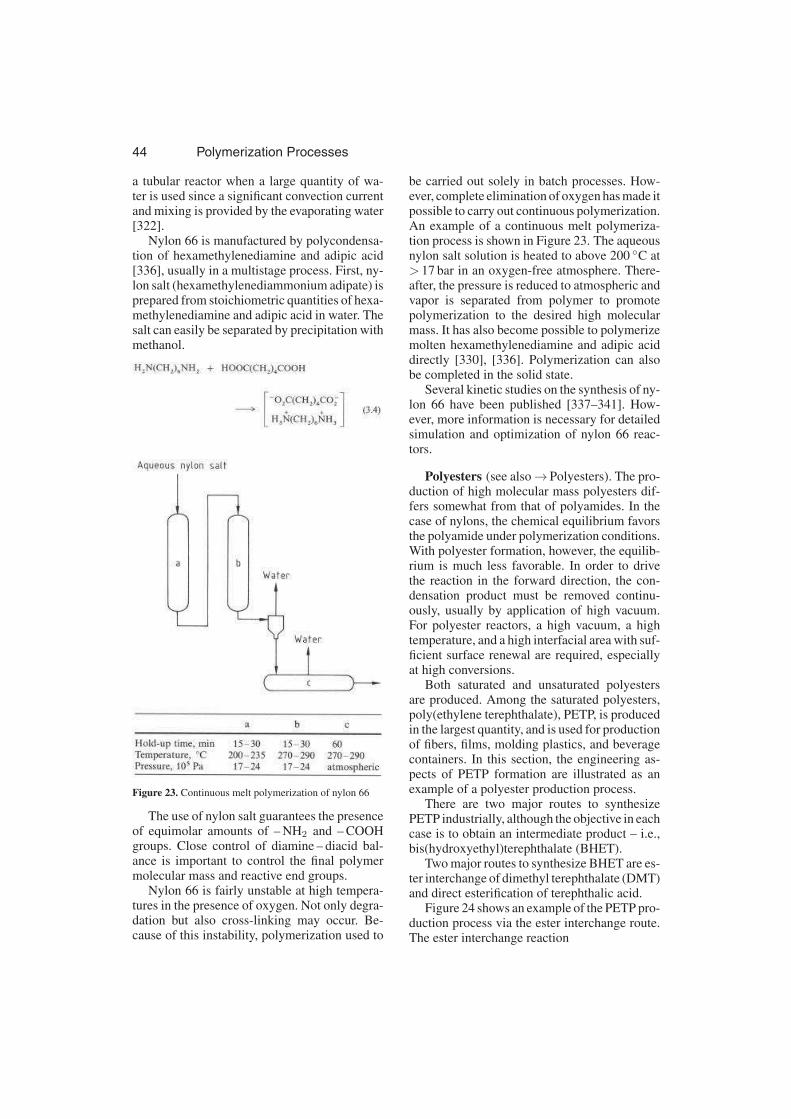
44 Polymerization Processes
a tubular reactor when a large quantity of wa-ter is used since a significant convection currentand mixing is provided by the evaporating water[322].
Nylon 66 is manufactured by polycondensa-tion of hexamethylenediamine and adipic acid[336], usually in a multistage process. First, ny-lon salt (hexamethylenediammonium adipate) isprepared from stoichiometric quantities of hexa-methylenediamine and adipic acid in water. Thesalt can easily be separated by precipitation withmethanol.
Figure 23. Continuous melt polymerization of nylon 66
The use of nylon salt guarantees the presenceof equimolar amounts of – NH2 and – COOHgroups. Close control of diamine – diacid bal-ance is important to control the final polymermolecular mass and reactive end groups.
Nylon 66 is fairly unstable at high tempera-tures in the presence of oxygen. Not only degra-dation but also cross-linking may occur. Be-cause of this instability, polymerization used to
be carried out solely in batch processes. How-ever, complete elimination of oxygen has made itpossible to carry out continuous polymerization.An example of a continuous melt polymeriza-tion process is shown in Figure 23. The aqueousnylon salt solution is heated to above 200 ◦C at> 17 bar in an oxygen-free atmosphere. There-after, the pressure is reduced to atmospheric andvapor is separated from polymer to promotepolymerization to the desired high molecularmass. It has also become possible to polymerizemolten hexamethylenediamine and adipic aciddirectly [330], [336]. Polymerization can alsobe completed in the solid state.
Several kinetic studies on the synthesis of ny-lon 66 have been published [337–341]. How-ever, more information is necessary for detailedsimulation and optimization of nylon 66 reac-tors.
Polyesters (see also→Polyesters). The pro-duction of high molecular mass polyesters dif-fers somewhat from that of polyamides. In thecase of nylons, the chemical equilibrium favorsthe polyamide under polymerization conditions.With polyester formation, however, the equilib-rium is much less favorable. In order to drivethe reaction in the forward direction, the con-densation product must be removed continu-ously, usually by application of high vacuum.For polyester reactors, a high vacuum, a hightemperature, and a high interfacial area with suf-ficient surface renewal are required, especiallyat high conversions.
Both saturated and unsaturated polyestersare produced. Among the saturated polyesters,poly(ethylene terephthalate), PETP, is producedin the largest quantity, and is used for productionof fibers, films, molding plastics, and beveragecontainers. In this section, the engineering as-pects of PETP formation are illustrated as anexample of a polyester production process.
There are two major routes to synthesizePETP industrially, although the objective in eachcase is to obtain an intermediate product – i.e.,bis(hydroxyethyl)terephthalate (BHET).
Two major routes to synthesize BHET are es-ter interchange of dimethyl terephthalate (DMT)and direct esterification of terephthalic acid.
Figure 24 shows an example of the PETP pro-duction process via the ester interchange route.The ester interchange reaction
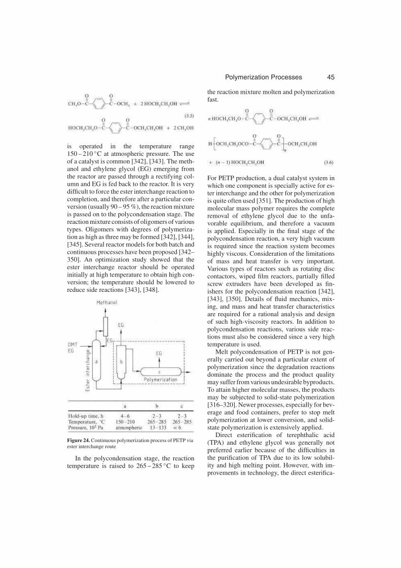
Polymerization Processes 45
is operated in the temperature range150 – 210 ◦C at atmospheric pressure. The useof a catalyst is common [342], [343]. The meth-anol and ethylene glycol (EG) emerging fromthe reactor are passed through a rectifying col-umn and EG is fed back to the reactor. It is verydifficult to force the ester interchange reaction tocompletion, and therefore after a particular con-version (usually 90 – 95 %), the reaction mixtureis passed on to the polycondensation stage. Thereaction mixture consists of oligomers of varioustypes. Oligomers with degrees of polymeriza-tion as high as three may be formed [342], [344],[345]. Several reactor models for both batch andcontinuous processes have been proposed [342–350]. An optimization study showed that theester interchange reactor should be operatedinitially at high temperature to obtain high con-version; the temperature should be lowered toreduce side reactions [343], [348].
Figure 24. Continuous polymerization process of PETP viaester interchange route
In the polycondensation stage, the reactiontemperature is raised to 265 – 285 ◦C to keep
the reaction mixture molten and polymerizationfast.
For PETP production, a dual catalyst system inwhich one component is specially active for es-ter interchange and the other for polymerizationis quite often used [351]. The production of highmolecular mass polymer requires the completeremoval of ethylene glycol due to the unfa-vorable equilibrium, and therefore a vacuumis applied. Especially in the final stage of thepolycondensation reaction, a very high vacuumis required since the reaction system becomeshighly viscous. Consideration of the limitationsof mass and heat transfer is very important.Various types of reactors such as rotating disccontactors, wiped film reactors, partially filledscrew extruders have been developed as fin-ishers for the polycondensation reaction [342],[343], [350]. Details of fluid mechanics, mix-ing, and mass and heat transfer characteristicsare required for a rational analysis and designof such high-viscosity reactors. In addition topolycondensation reactions, various side reac-tions must also be considered since a very hightemperature is used.
Melt polycondensation of PETP is not gen-erally carried out beyond a particular extent ofpolymerization since the degradation reactionsdominate the process and the product qualitymay suffer from various undesirable byproducts.To attain higher molecular masses, the productsmay be subjected to solid-state polymerization[316–320]. Newer processes, especially for bev-erage and food containers, prefer to stop meltpolymerization at lower conversion, and solid-state polymerization is extensively applied.
Direct esterification of terephthalic acid(TPA) and ethylene glycol was generally notpreferred earlier because of the difficulties inthe purification of TPA due to its low solubil-ity and high melting point. However, with im-provements in technology, the direct esterifica-

46 Polymerization Processes
Figure 25. Continuous polymerization process of PETP via direct esterification route
tion method has been gaining in importance. Theprocess is claimed to give polyesters with supe-rior quality due to their low content of carboxylend groups and diglycol linkages [351]. In themodeling of this process, aside from the diffi-culties caused by the various reactions and massbalances involved, it is necessary to take accountof the heterogenity of the reactions due to the lowsolubility of TPA in EG. Simulation and controlof the direct esterification reactors is reportedin [343], [350], [352–354]. Figure 25 shows aflow diagram of a continuous process for PETPproduction by direct esterification.
3.3. Processes and Reactor Modeling for
Chain-Growth Polymerization
3.3.1. Material Balance Equations for Batch,Semi-Batch, and Continuous Reactors
The following material balance equations ap-ply for multicomponent polymerization, accom-modate operation of a well-stirred reactor (nospatial variations in temperature and concentra-tions), and may be used to simulate different
comonomer systems under a variety of operat-ing conditions. Bulk (suspension) and solutionpolymerizations are considered first; extensionsrequired for multiphase systems (emulsion, in-verse emulsion, suspension, dispersion, and gas-phase processes) may be found elsewhere [355].Special cases where spatial variations in temper-ature and concentrations are important (e.g., intubular reactors or packed beds) are also consid-ered.
Bulk, solution, and suspension polymer-ization systems are characterized by the fact thatall of the reactions proceed in a single phasewith no spatial variations in temperature andconcentration. A model for a reactor carryingout such polymerizations would consist of a setof material balances giving the rates of accu-mulation, inflow, outflow and a reaction source(sink) term for the various monomers, initiators,chain-transfer agents, and polymer in the reac-tor. These balance equations are now given ingeneral form
Monomer balances:
dNi/dt=Fi, in− (Ni/V )Vout−RpiV (3.7)
Polymerization Processes 47
where
Ni is the number of moles of monomer i inthe reactor
Fi, in are molar flow rate of monomer i into thereactor
V is the reaction volume in the reactorVout is the total volumetric flow rate of all
species out of the reactorRpi is the net rate of disappearance of
monomer i by reaction
Reaction Volume. Since the density of a poly-mer is usually significantly greater than that of itsmonomer, the reaction volume V decreases withconversion for isothermal polymerization in abatch reactor. This shrinkage must also be takeninto account in semi-batch and continuous op-erations. Neglecting volume change on mixingpolymer and monomers (thermodynamic dataare most often not available and deviation fromideality is often not great) the change in reactionvolume (V ) may be calculated by using (assum-ing V is the equilibrium volume):
dV /dt=Vin−Vout−shrinkage rate
=Vs, in +
n∑
i=1
Fi, inMmi/mi
−
n∑
i=1
RpiMmi
(
1
mi
−1
p
)
V − Vout (3.8)
where n is the number of monomer types, V s, in
is the volumetric flow rate of inert solventinto the reactor, Mmi is the molecular mass ofmonomer i, mi
is the density of monomer i, p
is the density of polymer produced instanta-neously.
Polymer Balances. With a batch reactor,where there is no inflow and outflow of poly-mer from the reactor, the total amount of poly-mer formed and its composition can be obtaineddirectly from the monomer balances. However,with semi-batch and continuous operation, ad-ditional balances are required and these follow
dPi/dt=Fpi, in− (Pi/V )Vout +RpiV (3.9)
where Pi is the number of moles of monomer i
chemically bound in the polymer “in the reac-tor”, Fpi, in is the molar flow rate of monomer i
bound in the polymer flowing into the reactor.
Additional Ingredient Balances. In order tocalculate Rpi
for free-radical systems, the to-tal polymer radical concentration and, therefore,initiator concentration are required. In addition,balances for the chain-transfer agent (for mo-lecular mass calculations) and for the solventin solution polymerizations are required. Thesebalances follow:
dNIi/dt=FIi, in− (NIi/V )Vout−RIiV (3.10)
dVs/dt=Vs, in− (Vs/V )Vout (3.11)
dNT/dt=FT, in− (NT/V )Vout−RTV (3.12)
where N Ii is the number of moles of initiatorof type i in the reactor, FIi, in is the molar flowrate of initiator i into the reactor, RIi is the con-sumption rate of initiator i by reaction, V s is thevolume of inert solvent in the reactor, NT is thenumber of moles of chain-transfer agent (CTA)in the reactor, FT, in is the molar flow rate of CTAinto the reactor, and RT is the consumption rateof CTA by reaction.
It is convenient to sum the monomer bal-ance equation (Eq. 3.7) over n, the number ofmonomer types to give
dNM/dt=Fin− (NM/V )Vout−RpV (3.7a)
where NM is the total number of moles ofmonomer in the reactor, Fin is the total molarflow rate of monomer to the reactor, Rp is thetotal molar consumption rate of monomer by re-action.
3.3.1.1. Rates of Reaction and CopolymerComposition
With application of the pseudo-kinetic rate con-stant method, Rp can be expressed as
Rp =Kp [M] [P∗] (3.13)
where
[M] =NM/V =
n∑
i=1
[Mi] (3.13a)
and [Mi] is the concentration of monomer oftype i in the reactor.
When the terminal model [356] for copoly-merization is valid

48 Polymerization Processes
[P∗] =
n∑
i=1
[P∗i ] (3.13b)
where [P∗i ] is the concentration of active centersof type i in the reactor and
Kp =n∑
i=1
n∑
j=1
Kpijϕ∗i fj (3.13c)
where ϕ∗i is the number fraction of active cen-ters of type i in the reactor, and fj is the molefraction of monomer of type j in the reactor.
When the penultimate model [356] for co-polymerization is valid
[P∗] =n∑
ij
[
P∗ij]
(3.13d)
and
Kp =n∑
ijk
Kpijkϕ∗ijfk (3.13e)
The fraction of active centers of type i (ϕ∗i ) canbe found by using the stationary state hypoth-esis (SSH). Model development will continueassuming that the terminal model for copoly-merization is valid. The ϕ∗i may be found byusing
n∑
j=1j 6=i
Rpji =
n∑
j=1j 6=i
Rpij (3.14a)
with i = 1, . . . n and where Rpijis the consump-
tion rate of monomer j adding to the active centeri.
For anionic, cationic, and anionic coordina-tion polymerization, the estimation of the totalnumber of active centers is not always straightforward, and this quantity is sometimes used asan adjustable parameter. For free-radical poly-merization, a balance between radical genera-tion rate and bimolecular termination rates pro-vides the following with use of the SSH
[R·] =(
RI/KtN
)1/2(3.14b)
where [R•
] is the total concentration of poly-meric radicals in the reactor, RI is the generationrate of polymeric radicals of chain length unity,
and KtN is the number-average bimolecular ter-mination constant. When termination by com-bination and disproportionation are both signif-icant
KtN =KtcN +KtdN (3.14c)
For chemically controlled bimolecular termina-tion, pseudo-kinetic rate constants for KtcN andKtdN may be found in [355–357]. Details con-cerning the definitions and use of KtN, KtW,KtZ, may be found elsewhere [358], [359]. Thedefinition of KtN follows:
KtN =
∞∑
r=1
∞∑
s=1
Kt (r,s)ψ (r)ψ (s) (3.14d)
where Kt (r, s) is an arbitrary bimolecular termi-nation constant distribution for reaction of poly-meric radicals of chain length r and s and ψ (r)and ψ (s) are the number fractions of polymericradicals of chain length r and s. Note that KtN
can be used to calculate Rp and MN but if usedto calculate higher molecular mass averages theywould be underestimated if a significant numberof polymer chains are formed by bimoleculartermination reactions [358].
Realistic calculations of [R] using Equation(3.14 b) requires that the SSH be valid and thatdiffusion-controlled bimolecular termination beaccounted for. The first direct experimental testby ESR of the validity of the SSH for bulkpolymerization of methyl methacrylate (MMA)(where linear polymer chains are produced)and of MMA – ethylene glycol dimethacrylate(EGDMA) (where chains with long branchesand polymeric networks are formed) has shownthat SSH is valid for bulk MMA polymeriza-tion, but is not valid when substantial cross-linking occurs [360]. Coyle et al [361] haveconfirmed the validity of SSH for bulk poly-merization of MMA using numerical solutionsof the full set of kinetic equations. Attempts tomodel diffusion-controlled bimolecular termi-nation is considered later when discussing thepolymerization of MMA (see page 53) whichis considered the model system because of itsextreme Trommsdorff – Norrish effect. At veryhigh monomer conversions, when the polymer-ization temperature is below the glass transitiontemperature of the polymer being synthesized,the initiator efficiency and propagation constant
Polymerization Processes 49
both begin to fall dramatically, and these ef-fects should be properly accounted for. These ef-fects will also be considered in detail later whenMMA polymerization is discussed. The mod-eling of diffusion-controlled bimolecular termi-nation, propagation, and the cage effect on ini-tiator efficiency is not entirely clear, and muchresearch must be done before these topics maybe considered standard engineering practice.
The polymerization rates for individualmonomer type j can be calculated from
Rpj =
(
n∑
i=1
Kpijϕ∗i fj
)
[M] [P∗] (3.14e)
with j = 1, . . . n.The mole fraction of monomer of type j in
copolymer produced instantaneously is given by
Fj =Rpj /Rp (3.14f)
Monomer sequence length distributions may becalculated by using equations given in [356].
3.3.1.2. Molecular Masses, Long-ChainBranching, and Cross-Linking
Linear Copolymer Chains. For chainlengths greater than about 50 and when theterminal model for copolymerization is valid,Stockmayer’s bivariate weight chain lengthdistribution may be used to calculate the com-position and chain length of binary copolymerproduced instantaneously [356], [362]. The bi-variate distribution of the accumulated polymeris readily calculated by integrating the instan-taneous distribution using weighting factorsbased on instantaneous rates of polymer pro-duction. Unfortunately, an analytical functionfor a multidimensional distribution (involvingthree or more monomer types) has yet to bederived. However, part of this problem has al-ready been solved. In the limit of large chainlengths, the copolymer composition of chainsproduced instantaneously may be assumed tobe independent of chain length, and therefore,the instantaneous bivariate weight chain lengthdistribution is that given by the same expres-sion as for homopolymerization with all of thechains having the same composition Fi. Formore details, see Section 2.3.1 and [356].
Long-Chain Branching and Cross-Linking. The production of long branches andcross-links requires that so-called dead polymerchains take part in branching reactions to pro-duce tri- and tetrafunctional branch points viatransfer to polymer and by addition of polymerradical centers to polymer double bonds. Themechanisms of anionic, cationic, and anioniccoordination polymerization invariably producelinear polymer chains. There may be a few ex-ceptions, but these will not be considered.
Pseudo-kinetic rate constants for transfer topolymer and polymer radical addition to pendantdouble bonds may be defined as [355], [357],[363–365]
Kfp =
n∑
ij
KfpijϕiFj (3.15)
K∗p =
n∑
ij
K∗pijϕiFj (3.16)
when the terminal model is valid; where Fj
is the mole fraction of monomer j chemicallybound in the accumulated polymer. When a sig-nificant number of labile atoms have been ab-stracted and when a significant number of dou-ble bonds have been consumed, Equations (3.15)and (3.16) should be modified to account for this[363], [364].
When polymer chains that are normally inertto further reaction undergo long-chain branch-ing reactions, the instantaneous MWD is nolonger a permanent quantity. Therefore, themethod of moments should be used to calculatethe molecular mass averages. For details on theuse of the method of moments for the calcula-tion of sol molecular mass averages before andafter the gelation point and other methods forcalculating sol – gel fraction and cross-linkingdensity, see [363–365].
3.3.2. Examples of Free-RadicalPolymerization
3.3.2.1. Homopolymerization – LinearChains
The modeling techniques described in Section3.3.1 are illustrated with actual monomer sys-tems and experimental kinetic data. The sim-plest modeling examples (homopolymerization

50 Polymerization Processes
producing linear chains) are considered first, be-ginning with the thermal bulk polymerization ofstyrene, which is relatively easy to model and themodeling has been most successful in a varietyof applications.
Bulk Thermal Polymerization of Styrene(T> 100 ◦C). This system is comparativelyeasy to model for the following reasons:
1) The Mayo mechanism for thermal initiationof radicals is valid [366–368]
2) The polystyrene chains are linear3) The Trommsdorff – Norrish effect (see Sec-
tion 2.2.1.2), although significantly affectingthe polymerization rate, has at most a minoreffect on molecular mass development be-cause most of the polymer chains are pro-duced by chain transfer to the Diels – Alderintermediate [366].
The size of the polymeric radicals (radicalcenters are exclusively on chain ends) dependson temperature and monomer concentration (orconversion), and the molecular mass distribu-tion of the accumulated polymer differs littlefrom that of the polymeric radicals. In general,the self-diffusion coefficients of polymer radi-cals should depend on the size of the macrorad-ical, the concentration and MWD of the accu-mulated polymer, and temperature. The size ofthe macroradical is of greater importance thanthe MWD of the accumulated polymer [369],[370].
An empirical correlation of the bimoleculartermination constant with polymerization tem-perature and monomer conversion should pro-vide a model which is applicable over a rangeof process conditions (batch and continuous re-actor operation, temperature programming, etc).Another important factor, revealed in the work ofKirchner and Riederle [367], is that reactionsinvolved in thermal initiation do not becomediffusion controlled at monomer conversions ashigh as 97 %. The first effective model for thebulk thermal polymerization of styrene was de-veloped by Hui and Hamielec [371] and laterextended to higher temperatures (T < 230 ◦C)[372] and shown to be valid for a continuousstirred-tank reactor up to 280 ◦C [373]. Thismodel has been evaluated by many workers over
a wide range of reactor type and operational con-ditions. These include:
1) Wu et al. [374] used the model for a theo-retical/experimental optimization study em-ploying temperature programming in a batchreactor with highly successful results.
2) Kirchner et al. [375] applied the model toa CSTR and obtained accurate predictions.
3) Tien et al. [375] applied the model to a tubu-lar reactor with internal mixers.
4) DIERS [376], [377] (Design Institute forEmergency Relief Systems) a consortium ofchemical and insurance companies financedthe design and construction of a uniqueadiabatic reactor system (see Fig. 26) forthe measurement of temperature and pres-sure/time variations during adiabatic run-away exothermic reactions. They measuredresponses for the adiabatic thermal poly-merization of styrene (Fig. 27 and 28) andcompared them with those predicted bythe Hui – Hamielec polystyrene model andfound excellent agreement.
Figure 26. DIERS VSP (adiabatic batch reactor)–monitorstemperature and pressure changes during runaway of highlyexothermic reactions [377]a) Containment vessel (ca. 4 L); b) Test cell; c) Outer can;d) Guard heater; e) Inner heater; f) Insulation; g) Exhaustand supply; h) Bypass; i) Fill
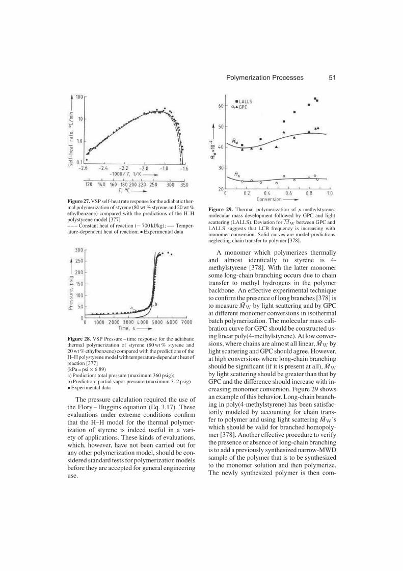
Polymerization Processes 51
Figure 27. VSP self-heat rate response for the adiabatic ther-mal polymerization of styrene (80 wt % styrene and 20 wt %ethylbenzene) compared with the predictions of the H–Hpolystyrene model [377]– – – Constant heat of reaction (− 700 kJ/kg); —- Temper-ature-dependent heat of reaction; •Experimental data
Figure 28. VSP Pressure – time response for the adiabaticthermal polymerization of styrene (80 wt % styrene and20 wt % ethylbenzene) compared with the predictions of theH–H polystyrene model with temperature-dependent heat ofreaction [377](kPa = psi× 6.89)a) Prediction: total pressure (maximum 360 psig);b) Prediction: partial vapor pressure (maximum 312 psig)•Experimental data
The pressure calculation required the use ofthe Flory – Huggins equation (Eq. 3.17). Theseevaluations under extreme conditions confirmthat the H–H model for the thermal polymer-ization of styrene is indeed useful in a vari-ety of applications. These kinds of evaluations,which, however, have not been carried out forany other polymerization model, should be con-sidered standard tests for polymerization modelsbefore they are accepted for general engineeringuse.
Figure 29. Thermal polymerization of p-methylstyrene:molecular mass development followed by GPC and light
scattering (LALLS). Deviation forMW between GPC andLALLS suggests that LCB frequency is increasing withmonomer conversion. Solid curves are model predictionsneglecting chain transfer to polymer [378].
A monomer which polymerizes thermallyand almost identically to styrene is 4-methylstyrene [378]. With the latter monomersome long-chain branching occurs due to chaintransfer to methyl hydrogens in the polymerbackbone. An effective experimental techniqueto confirm the presence of long branches [378] isto measure MW by light scattering and by GPCat different monomer conversions in isothermalbatch polymerization. The molecular mass cali-bration curve for GPC should be constructed us-ing linear poly(4-methylstyrene). At low conver-sions, where chains are almost all linear, MW bylight scattering and GPC should agree. However,at high conversions where long-chain branchingshould be significant (if it is present at all), MW
by light scattering should be greater than that byGPC and the difference should increase with in-creasing monomer conversion. Figure 29 showsan example of this behavior. Long-chain branch-ing in poly(4-methylstyrene) has been satisfac-torily modeled by accounting for chain trans-fer to polymer and using light scattering MW’swhich should be valid for branched homopoly-mer [378]. Another effective procedure to verifythe presence or absence of long-chain branchingis to add a previously synthesized narrow-MWDsample of the polymer that is to be synthesizedto the monomer solution and then polymerize.The newly synthesized polymer is then com-
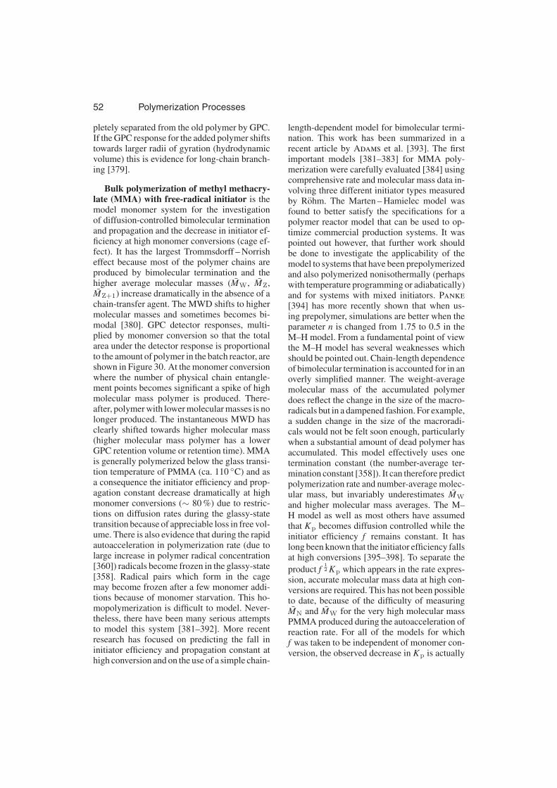
52 Polymerization Processes
pletely separated from the old polymer by GPC.If the GPC response for the added polymer shiftstowards larger radii of gyration (hydrodynamicvolume) this is evidence for long-chain branch-ing [379].
Bulk polymerization of methyl methacry-late (MMA) with free-radical initiator is themodel monomer system for the investigationof diffusion-controlled bimolecular terminationand propagation and the decrease in initiator ef-ficiency at high monomer conversions (cage ef-fect). It has the largest Trommsdorff – Norrisheffect because most of the polymer chains areproduced by bimolecular termination and thehigher average molecular masses (MW, MZ,MZ+1) increase dramatically in the absence of achain-transfer agent. The MWD shifts to highermolecular masses and sometimes becomes bi-modal [380]. GPC detector responses, multi-plied by monomer conversion so that the totalarea under the detector response is proportionalto the amount of polymer in the batch reactor, areshown in Figure 30. At the monomer conversionwhere the number of physical chain entangle-ment points becomes significant a spike of highmolecular mass polymer is produced. There-after, polymer with lower molecular masses is nolonger produced. The instantaneous MWD hasclearly shifted towards higher molecular mass(higher molecular mass polymer has a lowerGPC retention volume or retention time). MMAis generally polymerized below the glass transi-tion temperature of PMMA (ca. 110 ◦C) and asa consequence the initiator efficiency and prop-agation constant decrease dramatically at highmonomer conversions (∼ 80 %) due to restric-tions on diffusion rates during the glassy-statetransition because of appreciable loss in free vol-ume. There is also evidence that during the rapidautoacceleration in polymerization rate (due tolarge increase in polymer radical concentration[360]) radicals become frozen in the glassy-state[358]. Radical pairs which form in the cagemay become frozen after a few monomer addi-tions because of monomer starvation. This ho-mopolymerization is difficult to model. Never-theless, there have been many serious attemptsto model this system [381–392]. More recentresearch has focused on predicting the fall ininitiator efficiency and propagation constant athigh conversion and on the use of a simple chain-
length-dependent model for bimolecular termi-nation. This work has been summarized in arecent article by Adams et al. [393]. The firstimportant models [381–383] for MMA poly-merization were carefully evaluated [384] usingcomprehensive rate and molecular mass data in-volving three different initiator types measuredby Rohm. The Marten – Hamielec model wasfound to better satisfy the specifications for apolymer reactor model that can be used to op-timize commercial production systems. It waspointed out however, that further work shouldbe done to investigate the applicability of themodel to systems that have been prepolymerizedand also polymerized nonisothermally (perhapswith temperature programming or adiabatically)and for systems with mixed initiators. Panke
[394] has more recently shown that when us-ing prepolymer, simulations are better when theparameter n is changed from 1.75 to 0.5 in theM–H model. From a fundamental point of viewthe M–H model has several weaknesses whichshould be pointed out. Chain-length dependenceof bimolecular termination is accounted for in anoverly simplified manner. The weight-averagemolecular mass of the accumulated polymerdoes reflect the change in the size of the macro-radicals but in a dampened fashion. For example,a sudden change in the size of the macroradi-cals would not be felt soon enough, particularlywhen a substantial amount of dead polymer hasaccumulated. This model effectively uses onetermination constant (the number-average ter-mination constant [358]). It can therefore predictpolymerization rate and number-average molec-ular mass, but invariably underestimates MW
and higher molecular mass averages. The M–H model as well as most others have assumedthat Kp becomes diffusion controlled while theinitiator efficiency f remains constant. It haslong been known that the initiator efficiency fallsat high conversions [395–398]. To separate the
product f12 Kp which appears in the rate expres-
sion, accurate molecular mass data at high con-versions are required. This has not been possibleto date, because of the difficulty of measuringMN and MW for the very high molecular massPMMA produced during the autoacceleration ofreaction rate. For all of the models for whichf was taken to be independent of monomer con-version, the observed decrease in Kp is actually
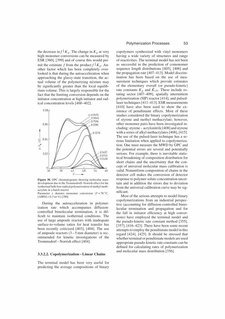
Polymerization Processes 53
the decrease in f12 Kp. The change in Kp at very
high monomer conversions can be measured byESR [360], [399] and of course this would per-
mit the estimate f from the product f12 Kp. An-
other factor which has been completely over-looked is that during the autoacceleration whenapproaching the glassy-state transition, the ac-tual volume of the polymerizing mixture maybe significantly greater than the local equilib-rium volume. This is largely responsible for thefact that the limiting conversion depends on theinitiator concentration at high initiator and rad-ical concentration levels [400–402].
Figure 30. GPC chromatograms showing molecular massdevelopment due to the Trommsdorff–Norrish effect for theisothermal bulk free-radical polymerization of methyl meth-acrylate in a batch reactorParameter x denotes monomer conversion (T = 70 ◦C,[AIBN] = 0.3 wt %) [380]
During the autoacceleration in polymer-ization rate which accompanies diffusion-controlled bimolecular termination, it is dif-ficult to maintain isothermal conditions. Theuse of large ampoule reactors with inadequatesurface-to-volume ratios for heat transfer hasbeen recently criticized [403], [404]. The useof ampoule reactors (3 – 5 mm diameter) is rec-ommended for kinetic investigations of theTrommsdorf – Norrish effect [404].
3.3.2.2. Copolymerization – Linear Chains
The terminal model has been very useful forpredicting the average compositions of binary
copolymers synthesized with vinyl monomershaving a wide variety of structures and rangeof reactivities. The terminal model has not beenas successful in the prediction of comonomersequence length distributions [405], [406] andthe propagation rate [407–413]. Model discrim-ination has been based on the use of mea-surement techniques which provide estimatesof the elementary overall (or pseudo-kinetic)rate constants Kp and KtN. These include ro-tating sector [407–409], spatially intermittentpolymerization (SIP) reactor [414], and pulsed-laser techniques [411–413]. ESR measurements[410] have also been used to show the ex-istence of penultimate effects. Most of thesestudies considered the binary copolymerizationof styrene and methyl methacrylate; however,other monomer pairs have been investigated in-cluding: styrene – acrylonitrile [408] and styrenewith a series of alkyl methacrylates [408], [415].The use of the pulsed-laser technique has a se-rious limitation when applied to copolymeriza-tion. One must measure the MWD by GPC andthe potential errors are several and potentiallyserious. For example, there is inevitable statis-tical broadening of composition distribution forshort chains and the uncertainty that the con-cept of universal molecular mass calibration isvalid. Nonuniform composition of chains in thedetector cell makes the conversion of detectorresponse to polymer solute concentration uncer-tain and in addition the errors due to deviationfrom the universal calibration curve may be sig-nificant.
Most of the serious attempts to model binarycopolymerizations from an industrial perspec-tive (accounting for diffusion-controlled bimo-lecular termination and propagation and forthe fall in initiator efficiency at high conver-sions) have employed the terminal model andthe pseudo-kinetic rate constant method [355],[357], [416–423]. There have been some recentattempts to employ the penultimate model in thisregard [424], [425]. It should be stressed thatwhether terminal or penultimate models are usedappropriate pseudo-kinetic rate constants can bedefined for calculating rates of polymerizationand molecular mass distribution [356].

54 Polymerization Processes
3.3.2.3. Copolymerization – Long-ChainBranching
The few serious attempts to model polymer-ization rate and molecular mass developmenthave employed the pseudo-kinetic rate con-stant method with the method of moments[355], [357], [363–365], [418], [419], [422]. Themethod of instantaneous MWD, which is such apowerful method for calculating the full MWDfor linear multicomponent polymers is not use-ful when dead polymer chains can be reactivatedduring formation of long-chain branches. Theinstantaneous MWD is no longer a permanentquantity but loses some of its chains, which be-come branched during the course of polymer-ization. It should be noted here that the pseudo-kinetic rate constant method is equally valid forthe modeling of linear and branched copoly-mer chain synthesis. The most common ana-lytical technique for the measurement of long-chain branching frequency (average number ofbranches per polymer molecule or per 1000backbone carbon atoms) is GPC with a dual de-tector system (mass concentration detector pluseither a viscometer or light scattering photome-ter as detector in series) or GPC with off-lineviscometry [426].
3.3.3. Polymerization Processes
3.3.3.1. Solution Polymerization
3.3.3.1.1. Polymer Soluble in Monomer
Kinetics. A polymerization in which thepolymer being synthesized is soluble in itsmonomer may be called a bulk or mass as well asa solution polymerization. A full description ofthe polymerization kinetics and modeling tech-niques can be found in Section 2.2.1 and Section3.3.2.
Polymerization Processes. The main tech-nical problems associated with solution poly-merization are heat removal, recovery of resid-ual monomer and solvent, and the manipula-tion of highly viscous solutions and melts. It iswell known that the ratio of cooling surface areato volume of reacting mixture decreases as thereactor volume increases. Length-to-diameter
ratios for reactors are usually < 2 to achieveacceptable mixing. When jacket cooling is nolonger sufficient to maintain isothermal poly-merization, additional modes of heat transfermust be used, as shown in Figure 31. Internalcooling coils are often not practical because theytend to interfere with stirring. External tubularcoolers can, in principle, provide a very largeheat-transfer area, but they may have very largepumping requirements in the case of highlyviscous solutions. Reflux cooling removes theheat of polymerization by evaporation of solventand/or monomer; the condensed vapor is recy-cled to the reacting mass. Condensers may be aslarge as necessary, with the limiting factor usu-ally the amount of vapor that can be treated with-out causing intense foaming or spattering of thepolymer solution. Remixing of the condensedliquid with the more viscous reacting mass mayalso be difficult.
3.3.3.1.2. Addition of a Solvent in whichboth Monomer and Polymer are Miscible
The addition of a solvent in which both monomerand polymer are miscible lowers the viscosityof the reacting mass, thereby improving its flowand heat-transfer characteristics. As a result, anddepending upon the nature and con-centrationof the solvent, the Trommsdorff – Norrish effectcan be either completely suppressed or signifi-cantly reduced. Use of solvent can be especiallybeneficial when evaporative cooling is used. Inchoosing a solvent, it is important to take into ac-count the possibility of chain transfer to solventwith a concomitant reduction in polymer mo-lecular mass. Removal of solvent and residual(unreacted) monomer from the highly viscouspolymer solution requires very high surface ar-eas to permit rapid devolatilization at the mod-erate temperatures required to minimize poly-merization and degradation of chains during de-volatilization to reduce off-spec polymer. Fig-ure 32 illustrates possible designs of devolatiliz-ers. One of these, the vacuum degasser, incorpo-rating a type of spray device [427], operates adia-batically, which means that the heat for evapo-ration is supplied by the solution itself. In con-trast, a degasser in series with a tubular heat ex-changer causes some of the monomer/solvent to
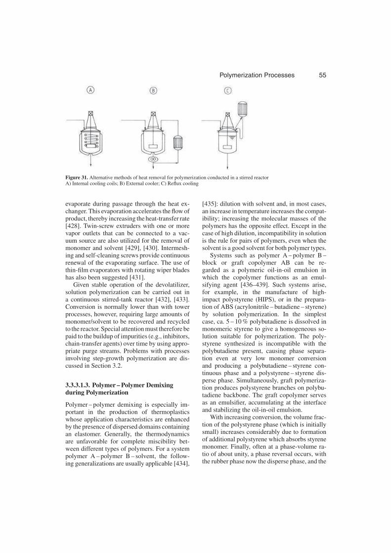
Polymerization Processes 55
Figure 31. Alternative methods of heat removal for polymerization conducted in a stirred reactorA) Internal cooling coils; B) External cooler; C) Reflux cooling
evaporate during passage through the heat ex-changer. This evaporation accelerates the flow ofproduct, thereby increasing the heat-transfer rate[428]. Twin-screw extruders with one or morevapor outlets that can be connected to a vac-uum source are also utilized for the removal ofmonomer and solvent [429], [430]. Intermesh-ing and self-cleaning screws provide continuousrenewal of the evaporating surface. The use ofthin-film evaporators with rotating wiper bladeshas also been suggested [431].
Given stable operation of the devolatilizer,solution polymerization can be carried out ina continuous stirred-tank reactor [432], [433].Conversion is normally lower than with towerprocesses, however, requiring large amounts ofmonomer/solvent to be recovered and recycledto the reactor. Special attention must therefore bepaid to the buildup of impurities (e.g., inhibitors,chain-transfer agents) over time by using appro-priate purge streams. Problems with processesinvolving step-growth polymerization are dis-cussed in Section 3.2.
3.3.3.1.3. Polymer – Polymer Demixingduring Polymerization
Polymer – polymer demixing is especially im-portant in the production of thermoplasticswhose application characteristics are enhancedby the presence of dispersed domains containingan elastomer. Generally, the thermodynamicsare unfavorable for complete miscibility bet-ween different types of polymers. For a systempolymer A – polymer B – solvent, the follow-ing generalizations are usually applicable [434],
[435]: dilution with solvent and, in most cases,an increase in temperature increases the compat-ibility; increasing the molecular masses of thepolymers has the opposite effect. Except in thecase of high dilution, incompatibility in solutionis the rule for pairs of polymers, even when thesolvent is a good solvent for both polymer types.
Systems such as polymer A – polymer B –block or graft copolymer AB can be re-garded as a polymeric oil-in-oil emulsion inwhich the copolymer functions as an emul-sifying agent [436–439]. Such systems arise,for example, in the manufacture of high-impact polystyrene (HIPS), or in the prepara-tion of ABS (acrylonitrile – butadiene – styrene)by solution polymerization. In the simplestcase, ca. 5 – 10 % polybutadiene is dissolved inmonomeric styrene to give a homogeneous so-lution suitable for polymerization. The poly-styrene synthesized is incompatible with thepolybutadiene present, causing phase separa-tion even at very low monomer conversionand producing a polybutadiene – styrene con-tinuous phase and a polystyrene – styrene dis-perse phase. Simultaneously, graft polymeriza-tion produces polystyrene branches on polybu-tadiene backbone. The graft copolymer servesas an emulsifier, accumulating at the interfaceand stabilizing the oil-in-oil emulsion.
With increasing conversion, the volume frac-tion of the polystyrene phase (which is initiallysmall) increases considerably due to formationof additional polystyrene which absorbs styrenemonomer. Finally, often at a phase-volume ra-tio of about unity, a phase reversal occurs, withthe rubber phase now the disperse phase, and the

56 Polymerization Processes
Figure 32. Options for removing residual monomer and solventA) Strand degasser; B) Tubular evaporator; C) Degassing extruder; D) Thin-film evaporator
polystyrene phase the continuous phase. Agita-tion is essential for the completion of phase re-versal, since rapid approach to equilibrium withrespect to transfer of monomer/polymer must beattained in a highly viscous medium. A commonresult of inadequate agitation is the interpenetra-tion of two continuous phases [438], [440–442].
Phase reversal can also lead to varioustypes of emulsions; e.g., polystyrene – styrenedroplets can be occluded within the rubber par-ticles of the disperse phase. This is actually de-sirable as it increases the volume fraction of thedisperse rubber phase. A reinforcing effect isobserved, with the resulting HIPS having higherimpact strength for a given mass of rubber incomparison with materials prepared by emul-sion grafting, in which occluded polystyrene isnot formed [443], [444]. Rather than rely on insitu formation of grafted rubber, it is also possi-ble from the outset to utilize block copolymersof styrene and butadiene as an additive in therecipe. The desired particle size distribution andmorphology of the rubber particles in HIPS isthen achieved by varying the intensity of agita-tion, the viscosities of the disperse and continu-ous phases, the graft activity of the primary rad-icals of the initiator, the molecular mass of thecontinuous phase, and the mass fraction and mo-lecular mass of the blocks in the diblock copoly-mer [445–454].
Figure 33 provides examples of the morphol-ogy of these rubber-modified polystyrene sys-tems. Morphologies of commercial significanceare essentially limited to cell and capsule struc-
tures, since the other morphologies shown gen-erally provide lower impact strength.
3.3.3.2. Precipitation Polymerization
The term precipitation polymerization refers toprocesses in which the initial ingredients ofa recipe are soluble, giving a homogeneoussolution, but the synthesized polymer precipi-tates during the course of polymerization. Theprecipitated polymer is generally swollen withmonomer and with nonsolvent if present. Toensure convenient handling the disperse phasemust be finely divided. This is achieved by ef-fective agitation, and a protective colloid (stericstabilizer) is often used. The associated prob-lems are similar to those with HIPS manufac-ture.
3.3.3.2.1. Polymer Insoluble in its Monomer
Polymers that are insoluble in their monomersinclude poly(vinyl chloride) and other polymersderived from halo or pseudohalo-substitutedethylenes such as vinyl bromide, vinylidenechloride, trifluoroethylene, and acrylonitrile.Polyethylene also falls into this category, at leastwhen produced under moderately high pressure.For the system vinyl chloride – poly(vinyl chlo-ride), for example, virtually no polymer dis-solves in the monomer in the temperature range30 – 60 ◦C. Solubility of the monomer in thepolymer is described well by the simplified

Polymerization Processes 57
Figure 33. Possible morphologies for rubber particles in impact resistant polystyrene [454]Length of the scale bar: 1 µm
Flory – Huggins equation (3.17) [435, p. 511],[455–457]:
ln
(
p
p0
)
= ln (1−ϕP) +ϕP +χϕ2p (3.17)
where
p0 is the vapor pressure of pure vinyl chloridep is the partial pressure of vinyl chlorideϕp is the volume fraction of poly(vinyl chlo-ride)χ is the polymer – solvent interaction param-eter.
According to [457], deviations from Equa-tion (3.17) are expected at low vapor pressures.The conversion – time curves for the bulk poly-merization of such monomer – polymer systemsall display rate increases with increasing con-version. This phenomenon has been especiallythoroughly investigated for the bulk polymer-ization of vinyl chloride. Its cause may be in-terpreted as follows: even at very low conver-sion, poly(vinyl chloride) precipitates, forminga monomer-swollen polymer-rich phase. Initia-tor is partitioned between the phases, and thusradical generation and polymerization occur inboth phases. The bimolecular termination rateis diffusion controlled in the polymer-rich phaseand hence the concentration of radicals is higherin this phase. Even though the monomer con-centration is lower in the polymer-rich phase,the specific polymerization rate Rp is higher. Inaddition, the volume of the polymer-rich phase
grows at the expense of the monomer-rich phasewith increasing monomer conversion. This ex-plains the autoacceleration in rate as monomerconversion increases.
Figure 34. Time – conversion curve for the bulk polymer-ization of vinyl chloride [459]Polymerization temperature 50 ◦C, initiator lauryl perox-ide, theoretical curves dashed[I]: • 0.78× 10⁻³ ; � 1.57× 10⁻³ ; △ 3.38×10⁻³ ; ×
5.50× 10⁻³ mol/mol vinyl chloride
Talamini has suggested that such a reac-tion may be described in terms of two homo-geneous polymerizations occurring in parallel,with rapid monomer transfer from the monomer-rich to the polymer-rich phase [458], [459]. As-suming that the monomer/polymer mass ratio inthe polymer-rich phase is independent of con-version or time, and that the ratio of the spe-cific polymerization rates in the two phases re-
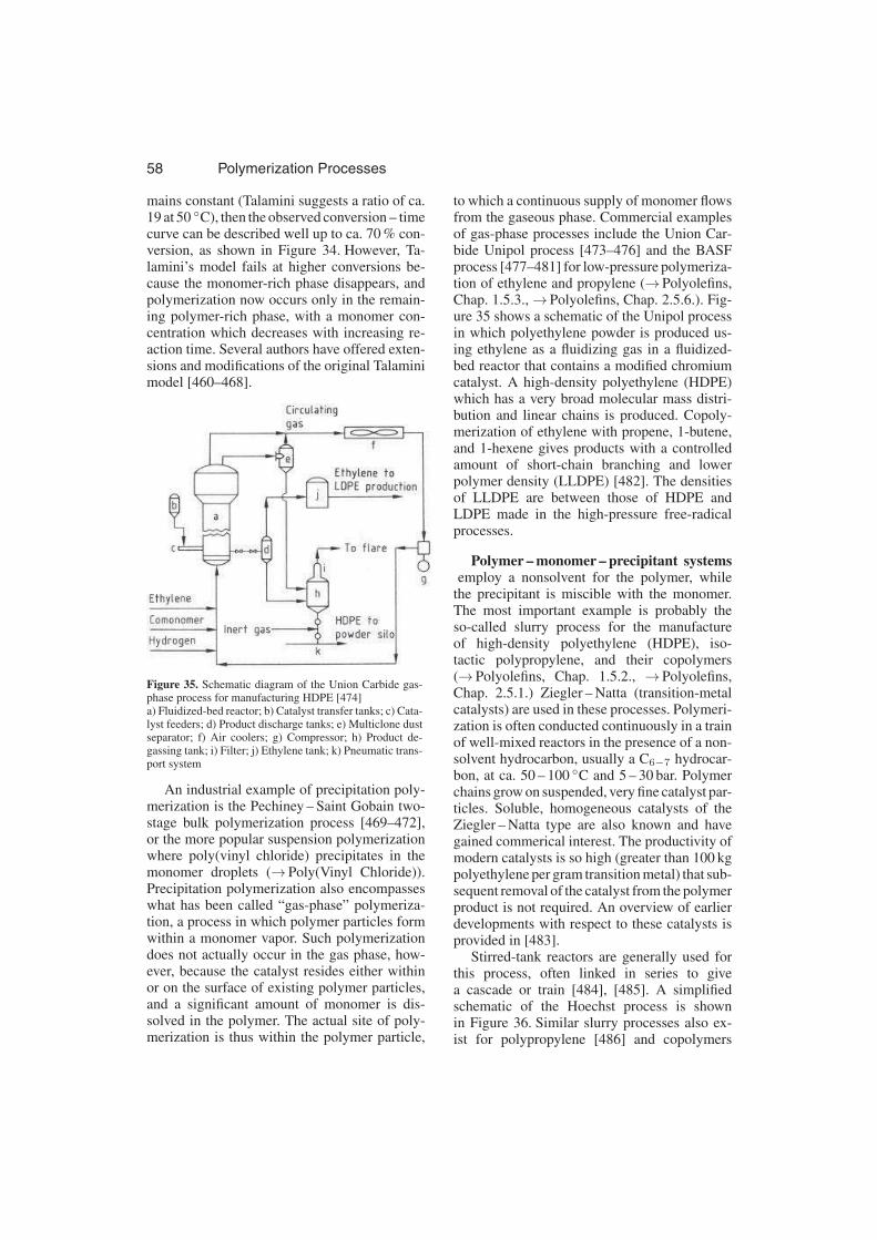
58 Polymerization Processes
mains constant (Talamini suggests a ratio of ca.19 at 50 ◦C), then the observed conversion – timecurve can be described well up to ca. 70 % con-version, as shown in Figure 34. However, Ta-lamini’s model fails at higher conversions be-cause the monomer-rich phase disappears, andpolymerization now occurs only in the remain-ing polymer-rich phase, with a monomer con-centration which decreases with increasing re-action time. Several authors have offered exten-sions and modifications of the original Talaminimodel [460–468].
Figure 35. Schematic diagram of the Union Carbide gas-phase process for manufacturing HDPE [474]a) Fluidized-bed reactor; b) Catalyst transfer tanks; c) Cata-lyst feeders; d) Product discharge tanks; e) Multiclone dustseparator; f) Air coolers; g) Compressor; h) Product de-gassing tank; i) Filter; j) Ethylene tank; k) Pneumatic trans-port system
An industrial example of precipitation poly-merization is the Pechiney – Saint Gobain two-stage bulk polymerization process [469–472],or the more popular suspension polymerizationwhere poly(vinyl chloride) precipitates in themonomer droplets (→Poly(Vinyl Chloride)).Precipitation polymerization also encompasseswhat has been called “gas-phase” polymeriza-tion, a process in which polymer particles formwithin a monomer vapor. Such polymerizationdoes not actually occur in the gas phase, how-ever, because the catalyst resides either withinor on the surface of existing polymer particles,and a significant amount of monomer is dis-solved in the polymer. The actual site of poly-merization is thus within the polymer particle,
to which a continuous supply of monomer flowsfrom the gaseous phase. Commercial examplesof gas-phase processes include the Union Car-bide Unipol process [473–476] and the BASFprocess [477–481] for low-pressure polymeriza-tion of ethylene and propylene (→Polyolefins,Chap. 1.5.3., →Polyolefins, Chap. 2.5.6.). Fig-ure 35 shows a schematic of the Unipol processin which polyethylene powder is produced us-ing ethylene as a fluidizing gas in a fluidized-bed reactor that contains a modified chromiumcatalyst. A high-density polyethylene (HDPE)which has a very broad molecular mass distri-bution and linear chains is produced. Copoly-merization of ethylene with propene, 1-butene,and 1-hexene gives products with a controlledamount of short-chain branching and lowerpolymer density (LLDPE) [482]. The densitiesof LLDPE are between those of HDPE andLDPE made in the high-pressure free-radicalprocesses.
Polymer – monomer – precipitant systemsemploy a nonsolvent for the polymer, while
the precipitant is miscible with the monomer.The most important example is probably theso-called slurry process for the manufactureof high-density polyethylene (HDPE), iso-tactic polypropylene, and their copolymers(→Polyolefins, Chap. 1.5.2., →Polyolefins,Chap. 2.5.1.) Ziegler – Natta (transition-metalcatalysts) are used in these processes. Polymeri-zation is often conducted continuously in a trainof well-mixed reactors in the presence of a non-solvent hydrocarbon, usually a C6−7 hydrocar-bon, at ca. 50 – 100 ◦C and 5 – 30 bar. Polymerchains grow on suspended, very fine catalyst par-ticles. Soluble, homogeneous catalysts of theZiegler – Natta type are also known and havegained commerical interest. The productivity ofmodern catalysts is so high (greater than 100 kgpolyethylene per gram transition metal) that sub-sequent removal of the catalyst from the polymerproduct is not required. An overview of earlierdevelopments with respect to these catalysts isprovided in [483].
Stirred-tank reactors are generally used forthis process, often linked in series to givea cascade or train [484], [485]. A simplifiedschematic of the Hoechst process is shownin Figure 36. Similar slurry processes also ex-ist for polypropylene [486] and copolymers

Polymerization Processes 59
Figure 36. Schematic of the Hoechst slurry-process for HPDE [484]a) Mixing vessels; b) Reactor; c) Postreactor; d) Centrifuge; e) Stripper; f) Dryer; g) Silo for HDPE powder
based on ethylene – propene (EPM) and ethyl-ene – propene – diene (EPDM) mixtures. Acry-lonitrile, sometimes together with a comonomer,can be polymerized in aqueous phase usinga redox system such as K2S2O8–Na2S2O5 orH2O2–Fe2+ [487]. The polymer precipitates asa fine powder, which is then filtered, washed,and dried. Dissolution of the polymer powderin dimethylformamide produces a spinning so-lution that can be used to produce polyacryloni-trile fibers. This process has been conducted in acontinuous manner [488]. One of the first com-mercial precipitation polymerizations was thebelt conveyor process for polyisobutylene devel-oped by BASF (Fig. 37; see also→Polyolefins,Chap. 4.2.4.). Equal amounts of isobutene andethylene are first mixed and then deposited inthe liquid state on a circulating steel belt. A sec-ond inlet is used to add a solution of BF3 inethylene. Cationic polymerization occurs veryrapidly, and the heat of polymerization is dissi-pated by the evaporation of ethylene. Thus, eth-ylene functions here not only as a precipitant butalso as a medium for evaporative cooling. Theresulting gaseous ethylene is purified, liquefied,and recycled.
A similar process is used by Exxon for thesynthesis of butyl rubber [489]. In this case, iso-prene serves as the comonomer and methyl chlo-ride takes the place of ethylene. Polymerizationis carried out in a continuous stirred-tank reac-tor. Residual monomer and diluent are removedfrom the resulting polymer suspension by strip-ping with hot water.
3.3.3.2.2. Monomer Functioning as Solventfor the Polymer
The Polymer – Monomer – PrecipitantSystem. If the polymer is soluble in itsmonomer, precipitation polymerization requiresthe addition of a precipitant that is miscible withthe monomer. Polymerization then begins in asolvent – nonsolvent mixture and it ends in aphase consisting only of pure precipitant onceconversion of the monomer is complete. Thus,the solubility relationships change during thecourse of the polymerization, and polymeriza-tion may initially occur in a homogeneous man-ner prior to the onset of precipitation, induced bythe enrichment in precipitant that accompaniesthe consumption of monomer.

60 Polymerization Processes
Figure 37. Schematic diagram of the BASF process for manufacturing polyisobutylene [433]a) Storage vessel for liquid isobutene; b) Storage vessel for liquid ethylene; c) Refrigerating condenser; d) Storage vesselfor ethylene containing 0.03 % boron trifluoride; e) Conveyor belt reactor; f) Heated degassing screw; g) Gaseous ethylene;h) Purification with calcium oxide ; i) Gasometer; j) Compressor
Figure 38. Volume-fraction ∗γprec (—-) of methanol as afunction of conversion for various initial concentrations ofmonomer [M]0 [491]Azeotropic precipitation copolymerization ofstyrene – acrylonitrile in methanol (– – –), precipita-tion point determined using cloud-point titration for twodifferent degrees of polymerization
Figure 38 illustrates these relationships, us-ing as an example the copolymerization (inmethanol as precipitant) of 40 mol % acryloni-trile and 60 mol % styrene (at the azeotropiccomposition). The volume fraction ∗γprec ofmethanol in the reaction mixture, defined as
∗γprec =
volumeof precipitant
volumeof precipitant + volumeof solvent(3.18)
is plotted in Figure 38 as a function of conversionfor various initial concentrations of monomer[M]0. The dashed lines represent extrapola-tions from experimental cloud-point titrationdata, which give the ∗γprec values at which thefirst polymer fractions precipitate at 65 ◦C. Foran initial concentration [M]0< 4.1 mol/L, ex-tremely small conversions suffice to cause pre-cipitation. At high monomer concentrations thepolymer initially remains in solution because thevolume fraction of methanol required for poly-mer precipitation has not yet been reached. Insuch cases, the critical value of ∗γprec is ex-ceeded only at higher conversion: the greater[M]0, the higher the conversion required.
In precipitation polymerization of this type itis especially important to ensure that the poly-mer precipitates in finely divided form. Amongother things this ensures that the particles donot overheat during polymerization. The pro-cess has been employed on large scale by BASF[490–492], with batch polymerization occur-ring in stirred reactors under reflux at 65 ◦C.Azobisisobutyronitrile was employed as inita-tor, and poly(vinyl pyrrolidone) or poly(vinylether) as a protective colloid. The resultingstyrene – acrylonitrile copolymer was separatedby centrifugation and the recovered methanolwas distilled and recycled to the next batch.

Polymerization Processes 61
Polymer dispersions in nonaqueous mediawith particle size in the range 0.01 – 10 µm (non-aqueous dispersions, colloids, organosols) havebeen thoroughly investigated by Barret andcoworkers [493]. Barret characterizes “disper-sion polymerization” as a process in which aninsoluble – and thus dispersed – polymer is pre-pared from a monomer dissolved in an organicdiluent to which has been added an amphiphaticblock or graft copolymer to serve as a dispersant.However, here this is regarded as a special caseof precipitation polymerization in which com-plete coagulation of polymer particles is pre-vented and the particle size is controlled.
The key to controlling particle size is the se-lection of dispersant type. Among the most ef-fective dispersing agents are the so-called am-phipathic molecules: block and graft copoly-mers made up of two polymeric components,only one of which is insoluble in the continu-ous, diluent-containing phase. Graft copolymersof this type often form during the polymerizationas a result of grafting on the dissolved polymer,but it is not absolutely essential that the insolubleportion of the dispersant be identical to or solu-ble in the disperse phase. In many cases its insol-ubility in the diluent is sufficient to ensure ade-quate adsorption on the particle surface. Theseamphipathic dispersing agents act as steric sta-bilizers [494].
Figure 39. Steric stabilization of precipitating poly-mer/monomer particles with the aid of amphipathic blockand graft copolymers [495]A) Schematic representation of adsorption of amphipathicmolecules on the polymer particles; —- insoluble groups,· · · · · soluble groups; B) Equilibrium established in thecourse of a precipitation polymerization P = (growing) poly-mer particle; C) Schematic representation of flocculationdue to multifunctional amphipathic molecules
Figure 39 A is a schematic representation ofthe adsorption of di-block, multiple-block, andgraft copolymers on the surface of growing poly-mer particles. Soluble and insoluble portions ofthe dispersant molecules must be kept carefullyin balance. If the insoluble part is too small, orif it interacts too weakly with polymer particles,then adequate adsorption will occur only whenthe dispersant concentration in the continuousphase is very high. If the soluble portion is toolarge, the dispersant will be present largely asaggregates or micelles with little tendency todissociate and be adsorbed on the interface. Fig-ure 39 B depicts the equilibrium situation. Fi-nally, it is important to note that multifunctionalamphipathic molecules like those shown in Fig-ure 39 C can also function as weak flocculatingagents.
In a well-stabilized dispersion, each particleis covered by a layer of freely moving poly-mer chains, which are in turn dissolved in thecontinuous phase. These layers prevent the fre-quently colliding particles from approaching soclosely that Van der Waal’s attractive forces be-come dominant. A simplified model (Fig. 40)suggests that the mechanism of steric stabiliza-tion involves an increase in the local concentra-tion of polymer chains or segments as a result ofoverlapping and mutual chain interpenetration[496] as two polymer particles approach. Thisinduces an osmotic pressure and increase in thefree energy ∆GR. To compensate for this effect,solvent flows into the regions of higher polymerconcentration and drives the particles apart. Apositive value of ∆GR = ∆HR−T ∆SR can bedue either to enthalpic effects (∆HR) or to en-tropic effects (T ∆SR). It is therefore possibleto divide the contributions to steric stabilizationinto three categories [498]:
1) Enthalpic stabilization∆HR and ∆SR are both positive∆HR>T ∆SR
The dispersion flocculates on warming2) Entropic stabilization
∆HR and ∆SR are both negativeT ∆SR>∆HR
The dispersion flocculates on cooling3) Combined enthalpic – entropic stabilization
∆HR is positive∆SR is negative

62 Polymerization Processes
The dispersion is stable over a wide range oftemperature.
Figure 40. Model for steric repulsion caused by the overlapof two spheres containing dissolved molecular chains [496],[497]C = Concentration of the polymer chains in the adsorptionlayers
More complete discussions of steric stabi-lization may be found elsewhere [495], [498–503]. A survey of precipitation polymerizationis available [504].
3.3.3.3. Suspension Polymerization
Definition. The term “suspension polymeriza-tion” includes a series of processes, all of whichinvolve emulsifying monomers to droplets bystirring them in a suspending medium in whichthey are insoluble in the presence of a free-radical initiator, usually one that is soluble inthe monomer. When the polymer formed issoluble in the monomer, nonporous spherical“beads” are formed, hence the term “suspensionbead polymerization”. If, however, the polymerprecipitates during polymerization, the result-ing polymer particles are composed of manysmaller primary particles. They are opaque, usu-ally possess an irregular surface, and may havesubstantial internal porosity. This type of poly-merization has been called “suspension pow-der polymerization”. The dispersants (protectivecolloids) are either macromolecules that are in-soluble in the suspending medium or insoluble,usually inorganic, powders, the so-called Pick-ering emulsifiers [505]. Their function is firstto assist in the formation of the initial monomeremulsion and then to stabilize the resulting poly-mer particle suspension. The following recipesare examples for suspension polymerization in-volving protective colloid and inorganic powderdispersants.
With protective colloid:
Temperature 80 ◦C
Reaction time 8 h
Styrene 100 parts (by mass)
Water 200 parts (by mass)
Benzoyl peroxide 0.4 parts (by mass)
Poly(vinyl alcohol)
[partially hydrolyzed poly(vinyl acetate)]
0.5 parts (by mass)
With pickering emulsifier:
Temperature 80 ◦C
Reaction time 10 h
Styrene 100 parts (by mass)
Water 200 parts (by mass)
Benzoyl peroxide 0.2 parts (by mass)
Barium sulfate 1.0 part (by mass)
C18SO3Na 0.002 parts (by mass)
The term “suspension polymerization” is per-haps inappropriate, because precipitation andemulsion polymerizations also produce suspen-sions of polymer particles in a continuous phase.The distinction from precipitation polymeriza-tion is that it is initiated in a homogeneousmixture, while suspension polymerization takesplace in an emulsion. The beads or powder par-ticles produced in a suspension polymerizationare roughly of the same size as the originalmonomer droplets with diameters on the or-der of 10−3 to 0.5 cm. Emulsion polymeriza-tion also starts with a monomer emulsion, butthe initiator is usually one that is soluble in thecontinuous suspending phase rather than in themonomer. Moreover, the resulting latex particlesare very much smaller (diameter range 5× 10⁻⁶
to 3× 10⁻⁵ cm or 0.05 to 0.3 µm) than the orig-inal monomer droplets. Borderline cases whichmight be called emulsion or suspension poly-merization are discussed later in Section 3.3.3.4.
In the vast majority of cases, the suspend-ing medium for suspension polymerization iswater, although inverse-suspension polymeriza-tions are also known and used commerciallyto produce very high molecular weight poly-mers and copolymers based on the comonomeracrylamide. Here a water-soluble monomer isdispersed in a hydrophobic organic suspendingmedium, usually in the presence of water in thedisperse phase.

Polymerization Processes 63
3.3.3.3.1. Qualitative Description
Generally, dispersants are employed at a con-centration (relative to the aqueous phase) of0.1 – 5 wt % in the case of protective colloidsand 0.1 – 2 wt % for Pickering emulsifiers. Atypical initiator concentration is 0.1 – 1 wt %relative to the monomer. The volume ratiomonomer/aqueous phase is usually between25 : 75 and 50 : 50, and the stereometric limit,which cannot be exceeded with spheres of uni-form size, is 74 : 26.
The reactor vessel is usually a stirred tank.The monomer is subjected either to turbulentpressure fluctuations or viscous shear forces,which break it into small droplets that assumea spherical shape under the influence of inter-facial tension. These droplets undergo constantcollision (collision rate ≥ 1 s−1), with some ofthe collisions resulting in coalescence. In the ab-sence of stabilizers, a dynamic equilibrium iseventually established, leading to a stationarymean particle size. Individual drops do not re-tain their unique identity, but instead undergocontinuous breakup and coalescence. This phe-nomenon can easily be demonstrated by the ad-dition of a small amount of a monomer that hasbeen labeled with a water-insoluble dye. The dyeis rapidly distributed uniformly in the dispersemonomer phase.
In some cases, an appropriate dispersant canbe used to induce the formation of a protectivefilm on the droplet surface. As a result, pairs orclusters of drops that tend to coalesce are bro-ken up by action of the stirrer before the crit-ical coalescence period elapses. A stable stateis ultimately reached in which individual dropsmaintain their identities over prolonged periodsof time. In this case, addition of dye-bearingmonomer does not result in migration of the dyeinto other droplets. Such a system is describedas a turbulence-stabilized emulsion.
In the simple case of a polymer that ismiscible in all proportions with its monomer(e.g., styrene and methyl methacrylate), variousviscosity states of the disperse phase are tra-versed during the course of polymerization. Theinitially nonviscous, liquid monomer is trans-formed gradually into an increasingly viscoussolution of polymer in monomer, and as conver-sion proceeds the disperse phase acquires thecharacteristics of a solid polymer. Particularly
in the tacky intermediate stage, individual poly-mer particles tend to form incompletely fusedclumps. Coagulation at this critical stage of con-version is somewhat inhibited by the action ofthe dispersant, but other effective measures to re-duce coagulation may also be taken, includingadjusting the densities of the two phases to makethem more similar, or by increasing the viscos-ity of the aqueous continuous phase. Rapid poly-merization during the sticky stage minimizes thenumber of collisions among polymer particlesand thus should reduce coagulation.
An experiment with dye-labeled monomer isalso applicable when polymerization occurs inthe disperse phase [506–508]. In this case dye-containing polymer beads generated in a paral-lel polymerization are added to the suspensionduring polymerization. It is observed that be-yond a certain conversion (which depends onthe reaction conditions) coagulation and parti-cle breakup cease entirely. This is known as the“particle identity point” or the limit of dynamicequilibrium. Increasing the dispersant concen-tration (i.e., reducing the size of particles) dis-places the identity point towards lower conver-sion [509], [510].
The schematic diagram in Figure 41 showsthese fundamental relationships. The upper partof the diagram corresponds to dynamic equilib-rium in a monomer emulsion that contains nodispersant, or to an emulsion undergoing poly-merization that has not yet reached the identitypoint. The monomer phase is broken up into longstrands by the stirrer, and these in turn fragmentinto spherical droplets due to interfacial tensionforces. The droplets may then agglomerate intolarger aggregates, finally coalescing into largerdrops, which either break apart again due to stir-ring or collect as an extended monomer phase.The lower portion of Figure 41 shows the var-ious stages that lie between the identity pointand the end of the polymerization process. Ina turbulence-stabilized emulsion, one in whichmonomer drops maintain their identity, the prob-ability is high that individual drops will poly-merize directly to primary beads. Nevertheless,even in a suspension bead polymerization, ir-regular particles sometimes appear, composedof many individual smaller polymer particles, aconsequence of some clusters surviving past theidentity point.
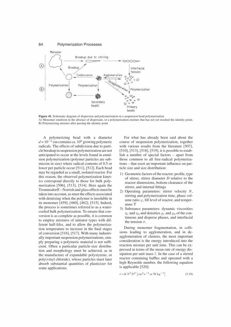
64 Polymerization Processes
Figure 41. Schematic diagram of dispersion and polymerization in a suspension bead polymerizationA) Monomer emulsion in the absence of dispersant, or a polymerization mixture that has not yet reached the identity point;B) Polymerizing mixture after passing the identity point
A polymerizing bead with a diameterd = 10−2 cm contains ca. 108 growing polymericradicals. The effects of subdivision due to parti-cle breakup in suspension polymerization are notanticipated to occur at the levels found in emul-sion polymerization (polymer particles are sub-micron in size) where radical contents of 0.5 orlower per particle occur [511], [512]. Each beadmay be regarded as a small, isolated reactor. Forthis reason, the observed polymerization kinet-ics correspond directly to those for bulk poly-merization [506], [513], [514]. Here again theTrommsdorff – Norrish and glass effects must betaken into account, as must the effects associatedwith demixing when the polymer is insoluble inits monomer [459], [460], [462], [515]. Indeed,the process is sometimes referred to as a water-cooled bulk polymerization. To ensure that con-version is as complete as possible, it is commonto employ mixtures of initiator types with dif-ferent half-lifes, and to allow the polymeriza-tion temperature to increase in the final stagesof conversion [516], [517]. With many industri-ally important suspension polymerizations, sim-ply preparing a polymeric material is not suffi-cient. Often a particular particle-size distribu-tion and morphology must be achieved, as inthe manufacture of expandable polystyrene, orpoly(vinyl chloride), whose particles must laterabsorb substantial quantities of plasticizer forsome applications.
For what has already been said about thecourse of suspension polymerization, togetherwith various results from the literature [507],[510], [513], [518], [519], it is possible to estab-lish a number of special factors – apart fromthose common to all free-radical polymeriza-tions – that exert an important influence on par-ticle size and size distribution:
1) Geometric factors of the reactor: profile, typeof stirrer, stirrer diameter D relative to thereactor dimensions, bottom clearance of thestirrer, and internal fittings
2) Operating parameters: stirrer velocity N ,stirring and polymerization time, phase vol-ume ratio ϕ, fill level of reactor, and temper-ature T
3) Substance parameters: dynamic viscositiesηc and ηd and densities c and d of the con-tinuous and disperse phases, and interfacialthe tension σ.
During monomer fragmentation, in colli-sions leading to agglomeration, and in de-agglomeration of clusters, the most importantconsideration is the energy introduced into thereaction mixture per unit time. This can be ex-pressed in terms of the mean rate of energy dis-sipation per unit mass ε. In the case of a stirredreactor containing baffles and operated with ahigh Reynolds number, the following equationis applicable [520]:
ε=KN3D2[
cm2 s−3 or Wkg−1]
(3.19)
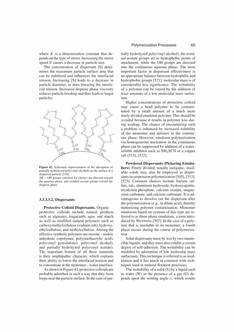
Polymerization Processes 65
where K is a dimensionless constant that de-pends on the type of stirrer. Increasing the stirrerspeed N causes a decrease in particle size.
The concentration of dispersant [S] deter-mines the maximum particle surface area thatcan be stabilized and influences the interfacialtension. Increasing [S] leads to a decrease inparticle diameter, as does lowering the interfa-cial tension. Increased disperse phase viscosityreduces particle breakup and thus leads to largerparticles.
Figure 42. Schematic representation of the adsorption ofpartially hydrolyzed poly(vinyl alcohol) on the surface of adispersed particle [510]All −OH groups (omitted for clarity) are directed towardthe aqueous phase, and residual acetate groups toward thedisperse phase
3.3.3.3.2. Dispersants
Protective Colloid Dispersants. Organicprotective colloids include natural productssuch as alginates, tragacanth, agar, and starchas well as modified natural polymers such ascarboxymethylcellulose (sodium salt), hydroxy-ethylcellulose, and methylcellulose. Among theeffective synthetic polymers are styrene – maleicanhydride copolymer, poly(methacrylic acid),poly(vinyl pyrrolidone), poly(vinyl alcohol),and partially hydrolyzed poly(vinyl acetate).The important feature of all these materialsis their amphipathic character, which explainstheir ability to lower the interfacial tension andto concentrate at the monomer – water interface.
As shown in Figure 42, protective colloids areprobably adsorbed in such a way that they formloops near the particle surface. In the case of par-
tially hydrolyzed poly(vinyl alcohol), the resid-ual acetate groups act as hydrophobic points ofattachment, while the OH groups are directedinto the continuous aqueous phase. The mostimportant factor in dispersant effectiveness isan appropriate balance between hydrophilic andhydrophobic groups [521]; molecular mass is ofconsiderably less significance. The wettabilityof a polymer can be varied by the addition oftrace amounts of a low molecular mass surfac-tant.
Higher concentrations of protective colloidmay cause a bead polymer to be contami-nated by a small amount of a much morefinely divided emulsion polymer. This should beavoided because it results in polymer loss dur-ing workup. The chance of encountering sucha problem is enhanced by increased solubilityof the monomer and initiator in the continu-ous phase. However, emulsion polymerizationvia homogeneous nucleation in the continuousphase can be suppressed by addition of a water-soluble inhibitor such as NH4SCN or a coppersalt [513], [522].
Powdered Dispersants (Pickering Emulsi-fiers). Finely divided, usually inorganic, insol-uble solids may also be employed as disper-sants in suspension polymerization [505], [513],[523]. Common choices include barium sul-fate, talc, aluminum hydroxide, hydroxyapatite,tricalcium phosphate, calcium oxalate, magne-sium carbonate, and calcium carbonate. It is ad-vantageous to dissolve out the dispersant afterthe polymerization (e.g., in dilute acid), therebyminimizing polymer contamination. Monomeremulsions based on systems of this type are re-ferred to as three-phase emulsions, a term intro-duced by Wenning [507]. In the case of a poly-mer that is insoluble in its monomer, a fourthphase occurs during the course of polymeriza-tion.
Solid dispersants must be wet by two immis-cible liquids, and they must also exhibit a certaindegree of self-adhesion. The wettability can bemodified by adsorption of low molecular masssurfactants. This technique is referred to as mod-ulation and it has much in common with tech-niques used in mineral flotation processes.
The wettability of a solid (S) by a liquid suchas water (W) in the presence of a gas (G) de-pends upon the wetting angle α, which results
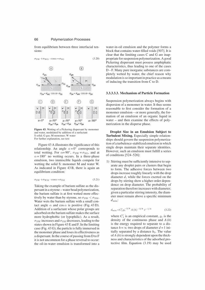
66 Polymerization Processes
from equilibrium between three interfacial ten-sions:
σSW +σWG · cosα=σSG (3.20)
Figure 43. Wetting of a Pickering dispersant by monomerand water, modulated by addition of a surfactantS solid; G gas; M monomer; W waterFor further explanation, see text
Figure 43 A illustrates the significance of thisrelationship. An angle α = 0◦ corresponds tototal wetting. For α= 90◦, σSW =σSG, and atα = 180◦ no wetting occurs. In a three-phaseemulsion, two immiscible liquids compete forwetting the solid S: monomer M and water W.As indicated in Figure 43 B, there is again anequilibrium condition:
σSW +σWM · cosα=σSM (3.21)
Taking the example of barium sulfate as the dis-persant in a styrene – water bead polymerization,the barium sulfate is at first wetted more effec-tively by water than by styrene, so σSW<σSM.Water wets the barium sulfate with a small con-tact angle α and cosα is positive (Fig. 43 D).Addition of a surfactant whose polar groups areadsorbed on the barium sulfate makes the surfacemore hydrophobic (or lypophilic). As a result,σSW increases andσSM decreases, leading to thestates shown in Figure 43 E and F. In the limitingcase (Fig. 43 G), the particle is fully immersed inthe monomer phase and loses its effectiveness asa dispersant. In the course of passing from D to Fit is not uncommon for a phase reversal to occur:the oil-in-water emulsion is transformed into a
water-in-oil emulsion and the polymer forms ablock that contains water-filled voids [507]. It isclear that the limiting cases C and G are inap-propriate for suspension polymerization. A goodPickering dispersant must possess amphiphaticcharacteristics, thus leading to one of the casesD – F. Many pure inorganic substances are com-pletely wetted by water, the chief reason whymodulation is so important in practice as a meansof inducing the transition from C to D.
3.3.3.3.3. Mechanism of Particle Formation
Suspension polymerization always begins withdispersion of a monomer in water. It thus seemsreasonable to first consider the formation of amonomer emulsion – or more generally, the for-mation of an emulsion of an organic liquid inwater – and then examine the effects of poly-merization in the disperse phase.
Droplet Size in an Emulsion Subject toTurbulent Mixing. Especially simple relation-ships should govern the suspension polymeriza-tion of a turbulence-stabilized emulsion in whichsingle drops maintain their separate identities.However, such an emulsion must fulfill a seriesof conditions [524–526]:
1) Stirring must be sufficiently intensive to sep-arate any droplet pairs or clusters that beginto form. The adhesive forces between twodrops increase roughly linearly with the dropdiameter d, while the forces exerted on thedrops by stirring show a higher order depen-dence on drop diameter. The probability ofseparation therefore increases with diameter;given a particular stirring intensity, the diam-eter must remain above a specific minimumdmin:
dmin =C′1−3/8c A (h)−3/8 ε−1/4 (3.22)
where C′1 is an empirical constant, c is thedensity of the continuous phase and A (h)is the energy required to separate to a dis-tance h =∞ two drops of diameter d = 1 ini-tially separated by a distance h0. The valueof A (h) is strongly dependent upon the thick-ness and characteristics of the adsorbed pro-tective film. Equation (3.19) may be used
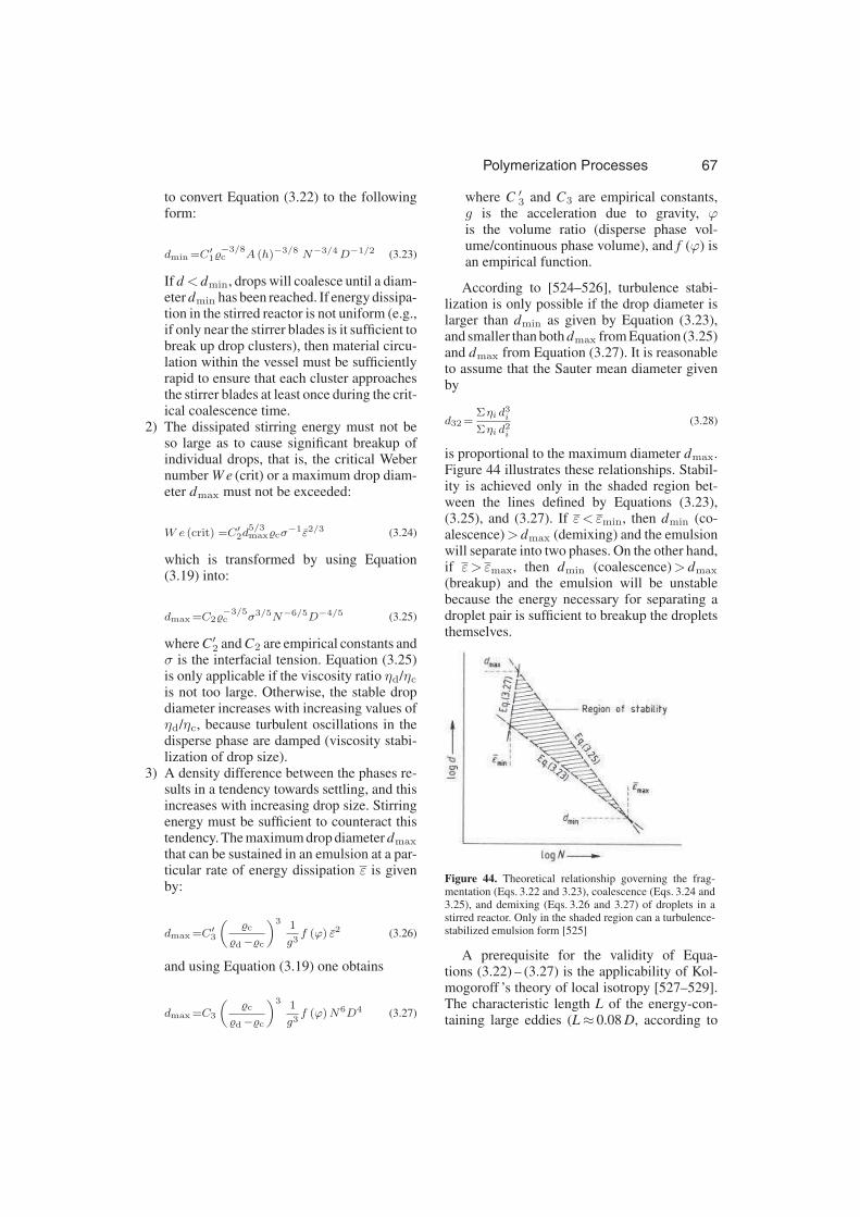
Polymerization Processes 67
to convert Equation (3.22) to the followingform:
dmin =C′1−3/8c A (h)−3/8 N−3/4D−1/2 (3.23)
If d< dmin, drops will coalesce until a diam-eter dmin has been reached. If energy dissipa-tion in the stirred reactor is not uniform (e.g.,if only near the stirrer blades is it sufficient tobreak up drop clusters), then material circu-lation within the vessel must be sufficientlyrapid to ensure that each cluster approachesthe stirrer blades at least once during the crit-ical coalescence time.
2) The dissipated stirring energy must not beso large as to cause significant breakup ofindividual drops, that is, the critical Webernumber W e (crit) or a maximum drop diam-eter dmax must not be exceeded:
W e (crit) =C′2d5/3maxcσ
−1ε2/3 (3.24)
which is transformed by using Equation(3.19) into:
dmax =C2−3/5c σ3/5N−6/5D−4/5 (3.25)
where C′2 and C2 are empirical constants andσ is the interfacial tension. Equation (3.25)is only applicable if the viscosity ratio ηd/ηc
is not too large. Otherwise, the stable dropdiameter increases with increasing values ofηd/ηc, because turbulent oscillations in thedisperse phase are damped (viscosity stabi-lization of drop size).
3) A density difference between the phases re-sults in a tendency towards settling, and thisincreases with increasing drop size. Stirringenergy must be sufficient to counteract thistendency. The maximum drop diameter dmax
that can be sustained in an emulsion at a par-ticular rate of energy dissipation ε is givenby:
dmax =C′3
(
c
d−c
)3 1
g3f (ϕ) ε2 (3.26)
and using Equation (3.19) one obtains
dmax =C3
(
c
d−c
)3 1
g3f (ϕ)N6D4 (3.27)
where C ′3 and C3 are empirical constants,
g is the acceleration due to gravity, ϕis the volume ratio (disperse phase vol-ume/continuous phase volume), and f (ϕ) isan empirical function.
According to [524–526], turbulence stabi-lization is only possible if the drop diameter islarger than dmin as given by Equation (3.23),and smaller than both dmax from Equation (3.25)and dmax from Equation (3.27). It is reasonableto assume that the Sauter mean diameter givenby
d32 =Σηi d
3i
Σηi d2i(3.28)
is proportional to the maximum diameter dmax.Figure 44 illustrates these relationships. Stabil-ity is achieved only in the shaded region bet-ween the lines defined by Equations (3.23),(3.25), and (3.27). If ε< εmin, then dmin (co-alescence)> dmax (demixing) and the emulsionwill separate into two phases. On the other hand,if ε> εmax, then dmin (coalescence)> dmax
(breakup) and the emulsion will be unstablebecause the energy necessary for separating adroplet pair is sufficient to breakup the dropletsthemselves.
Figure 44. Theoretical relationship governing the frag-mentation (Eqs. 3.22 and 3.23), coalescence (Eqs. 3.24 and3.25), and demixing (Eqs. 3.26 and 3.27) of droplets in astirred reactor. Only in the shaded region can a turbulence-stabilized emulsion form [525]
A prerequisite for the validity of Equa-tions (3.22) – (3.27) is the applicability of Kol-mogoroff ’s theory of local isotropy [527–529].The characteristic length L of the energy-con-taining large eddies (L≈ 0.08 D, according to

68 Polymerization Processes
[244]) must be larger, and the characteristiclength l of the energy-dissipating small ed-dies [l = (γ3
c /ε)1/4], where γc is the kinematicviscosity of the continuous phase] must bemuch smaller than the drop diameter d (i.e.,L≫ d≫ l). Equations (3.24) and (3.25) [531–534] as well as (3.22) and (3.23) [525], [526],[535] have been verified experimentally. Nev-ertheless, they apply only for very small phaseratiosϕ< 0.015, which are unrealistic for indus-trial suspension polymerizations. The polymer-izing system is also subject to nonnegligible ef-fects of the viscosity ratio ηd/ηc. In [536], for ex-ample, this has been taken into account by intro-duction of the viscosity group ηd(d σ d)−1/2,which depends only on the physical propertiesof the disperse phase. At higher phase ratios,both d32 and dmax increase with increasing dis-tance from the stirrer [534], [537], [538]. Variouscorrections [531], [534], [539], [540] have beensuggested for Equation (3.25), all of which takethe form:
d32
D=A (1+Bϕ) W e−3/5 (3.29)
where A and B are numerical constants. Forphase relationships such as those applicable onan industrial scale it is therefore not possible toassume a homogeneous energy-dissipation rateε; instead, it must be anticipated that ε is largein the vicinity of the stirrer, becoming smallerin more remote circulation zones. A simulationprogram has been described [541–543] that ap-proaches this problem by dividing the reactorinto various stirring and circulation zones andthen applying Monte Carlo methods.
The Size of the Polymer Particles. Con-version of a monomer into polymer increasesthe viscosity ηd and density d of the dispersephase, and lowers the volume phase ratio ϕ. Theinterfacial tension σ also changes, and graftingreactions between polymeric radicals on the or-ganic protective colloid and the monomer mayhave to be accounted for. As has been demon-strated by Hopff et al. [544–547] in the caseof a suspension bead polymerization of methylmethacrylate with a relatively high concentra-tion of a protective colloid [poly(vinyl alcohol),Mowiol N 70 (88)], systems exist in which thefinal particle size is already established at verylow conversion. Polymerizing droplets main-tain their identity, and subsequent reduction
in stirring speed has no influence on particlesize. Apparently, a turbulence-stabilized stateis reached at the very onset of polymerization.Evaluation with respect to particle size is partic-ularly straightforward in this case, since changesin the above-mentioned parameters during poly-merization are irrelevant.
A series of experiments in geometrically sim-ilar reactors (see Fig. 45) coupled with dimen-sional analysis, permitted derivation of the fol-lowing dimensionless equation in the case of thisespecially simple system:
d50
D=kRe0.5W e−0.9Fr−0.1
(
ηd
ηc
)0.1
ϕ0 (3.30)
where d50 is the bead diameter below which50 wt % of the particles pass through the sieve(in other words 50 wt % of the particles have adiameter less than d50), D is the stirrer diameter,which throughout the experiments was kept in aconstant ratio to the reactor diameter, and k is anumerical constant.
Figure 45. Dependence of the bead diameter d50 on thestirrer velocity N [545]Experiments conducted in four geometrically similar stirredreactors with stirrer diameter D
Curve parameter: protective colloid concentration ing/100 cm3
The dimensionless groups are:
Polymerization Processes 69
Re=
(
D2Nc
ηc
)
= ratio of inertial/viscous forces
Fr=
(
DN2
g
)
=
ratio of inertial/gravitational forces (3.30a)
W e=
(
D3N2c
σ
)
=
ratio of inertial/interfacial forces
It follows that d50 = kN−1.5
A relationship similar to Equation (3.30) hasbeen found for the suspension polymerizationof vinyl chloride [548], [549]. In this case, how-ever, a large particle diameter region was identi-fied with d = kN−1.9 at low stirrer speeds (withcorrespondingly large particle diameters) as wellas a fine-particle size region with d = kN−0.6.An analogous effect has also been reported forstyrene [550].
In contrast to the very early establishment ofparticle diameter in the experiments of Hopff etal., dye-labeling experiments have shown that inother systems [506–508], [550], [551] the par-ticles reach the so-called identity point only athigh conversion. With these systems it is appar-ently necessary to take into account the time andconversion dependence of the parameters enu-merated above. Another important observation[550], [552] is the fact that in certain systems thestirring time in which the unpolymerized emul-sion reaches its final droplet diameter is longerthan that taken by the polymerizing system toreach 50 % conversion. A faster polymerizationwould therefore give larger polymer particlesdue to viscosity stabilization.
The problems associated with scaling upfrom small to industrial scale, particularly forparticle size, are an important concern in sus-pension polymerization. In principle, Equation(3.30) should be applicable, suggesting that allthat is required for maintaining constant d/Dwhen scaling up is to keep Re, W e, Fr, and ηd/ηc
constant. However, Equations (3.30 a) show thatthis is not possible without changing the com-position of the system. Furthermore, it is d, notd/D, that must be kept constant in an industrialscaleup. To what extent it is possible at highReynolds numbers to avoid an exact similaritytransformation and scale the process up on thebasis, for example, of [553], [554]
d
D=kW e−0.6Eu−1.0 (3.31)
or
d∼D−0.8N−1.2 (3.32)
has not yet been established experimentally (Eu
is here a modified power number in power perunit volume). A not further defined suspensionpolymerization of methyl methacrylate in 1 %polyacrylamide solution was transformed withconstant particle size on the basis of
N1 =N2
(
D2
D1
)2/3
(3.33)
from a laboratory reactor (1) with D = 10.1 cmto a half-tonne scale (2) with D = 81.2 cm [555].
3.3.3.3.4. Industrial Applications
Suspension polymerization is used for produc-ing a wide variety of polymer types, the mostimportant of which are mentioned briefly. Stan-dard polystyrene for use in injection moldingis manufactured by suspension bead polymer-ization, as is poly(methyl methacrylate) and itscopolymers containing small amounts of acry-late esters. Clear transparent polymers are of-ten required, so formulations involving Picker-ing dispersant (e.g., MgCO3) that can be dis-solved out of the polymer with dilute acid afterpolymerization are particularly advantageous.
In the case of styrene – acrylonitrile copoly-mers, the method of choice for batch suspen-sion polymerization is normally that involvingthe azeotropic composition to minimize compo-sitional drift. Nevertheless, complications oftenarise, because considerably more acrylonitrilethan styrene dissolves in the aqueous contin-uous phase. As conversion proceeds, acryloni-trile diffuses into the polymer particles and themonomer ratio in the beads changes, causingthe composition of the copolymer to change aswell [556]. The same phenomenon can accom-pany copolymerization in heterogeneous sys-tems generally [557].
High-impact polystyrene and ABS are oftenprepared in a combined process. This beginswith a solution of polybutadiene in styrene or
70 Polymerization Processes
styrene/acrylonitrile and permits bulk polymer-ization to occur under stirring until phase rever-sal or inversion has occurred. Water and disper-sant are then added and the polymerization iscompleted in suspension [558], [559].
Expandable polystyrene is prepared by sus-pension polymerization in the presence of ablowing agent, such as pentane [560], [561]. Itis also possible to introduce the blowing agent ina second step after polymerization, allowing itto diffuse into the beads [562], [563]. Warmingto 80 – 110 ◦C, generally with steam, causes thebeads to expand by foaming, their volume in-creasing by a factor of ca. 30 – 50. Particle sizeand size distributions both play important roles.For example, if thin-walled objects are to bemade from expandable polystyrene, especiallysmall polymer particles are required. The un-foamed product is fractionated by sieving priorto drying. Figure 46 shows a schematic of a typ-ical EPS production facility.
Figure 46. Schematic representation of the manufacture ofStyropor by batch suspension polymerizationa) Mixing tank; b) Stirred reactor; c) Puffer tank; d) Cen-trifuge; e) Sieving; f) Drying; g) Silo; h) Packaging
The required amount of deionized water isloaded into the reactor at ambient temperatureand agitation is started. Styrene and the initiatorpair, AIBN or benzoyl peroxide plus a finishinginitiator such as di-tert-butyl peroxide or tert-butyl peroxybenzoate are pumped into the reac-tor at a constant rate, while the stabilizer, eitheran inorganic, insoluble, finely divided powder ora polymeric steric stabilizer is added. The reac-tor is closed and the heating cycle starts. Dropletsize development occurs during the heating cy-cle. When the polymerization temperature isreached, between 75 ◦C and 95 ◦C depending onthe initiator type, the polymerization proceedsuntil a conversion in the range 32 – 35 % is ob-
tained. This point marks the beginning of theso-called “sticky-stage” at which point the co-alescence rate begins to increase, causing thebeads to grow from a mean particle diameterof about 0.2 mm to the desired size, dependingon the original stabilizer formulation, for the fi-nal application of the resin product. During thisstage of the process, particle size is monitoredby periodic sampling of particle size growthrate. Additional stabilizer may be added if thegrowth rate is too large. At 65 – 68 % conver-sion of monomer, the identity point is reached.At this point the particle viscosity is sufficientlylarge that collisions between particles are elas-tic and particle size growth ceases. In addition,the density of dispersed and continuous phasesare almost identical, and the suspension is verystable. Autoacceleration of the polymerizationrate becomes appreciable at the identity pointand increases until ca. 95 % conversion where aglassy-state transition occurs and the beads be-come hard. Once the beads are hard the reac-tion mixture is heated to a temperature abovethe glass transition temperature of the polysty-rene (Tg≈ 100 ◦C). During heating, the reactoris pressurized with a blowing agent (5 – 8 % withrespect to polymer), a low-boiling hydrocarbon(C4 – C7). The reactor is then pressurized withnitrogen at 700 – 950 kPa and the so-called im-pregnation stage starts and proceeds for 3 – 8 h.During impregnation the blowing agent diffusesinto the beads. At the same time, the free vol-ume increases, and the finishing initiator rapidlygenerates radicals, causing a relatively rapid in-crease to a monomer conversion of ca. 99.9 %.The impregnation time should be sufficient toallow the blowing agent to reach the core of theparticle and to cause the breakup of hydrocarbondomains within the polymer matrix, giving a uni-form distribution. At the end of the impregnationstage the suspension is cooled to 20 – 30 ◦C, de-pending on the blowing agent type, to freeze inthe ingredients and prevent bead expansion dur-ing handling. Some typical properties of an EPSgrade are:
Monomer conversion > 99.9 %
MW× 10−3 200 – 300
Polydispersity 2.2 – 2.4
Mean particle diameter d 0.4 – 1.5 mm
PSD breadth σ/d 0.20 – 0.25
Blowing agent concentration 5.0 – 8.0 %

Polymerization Processes 71
Table 3 lists required properties of the beadfor different applications.
Table 3. EPS bead properties and applications
d, mm σ/d Density, kg/m3 Use
1.5 0.20 8 – 16 construction
(insulation)
1.0 0.15 12 – 20 packaging
0.4 0.10 50 – 70 coffee cups
Figure 47. Growth path for EPS beads (mean diameter d
versus monomer conversion) during suspension polymer-ization of styrene [564]Stage I: breakup and coalescence rates are about equalStage II: coalescence rate exeeds breakup rateStage III: conversions exceed identity point (no furtherbreakup and coalescence)
Suspension polymerization processes give arather broad PSD. In some EPS applications,such as for coffee cups, a very narrow PSD isrequired and for this grade the suspension poly-merization process is commonly carried out intwo stages to minimize off-spec resin. In the firststage, styrene is polymerized to give the nar-rowest PSD possible and then the suspension isremoved from the reactor and the polymer par-ticles are classified by sieving to give the re-quired narrow PSD. The particles are then re-suspended in the reactor to permit impregnationwith a blowing agent in the second stage. Sus-pension polymerization for EPS production is athree stage process. In the first stage, the parti-cle viscosities are low and an equilibrium par-ticle size is obtained (rates of droplet breakupand coalescence are equal). In the second stage,where the viscosity of the particles is sufficientlyhigh, the particles grow (coalescence rate ex-ceeds breakup rate). For EPS, Villalobos [564]
observed that no further breakup occurs beyond50 % monomer conversion when the particle vis-cosity is about 104 cP. Addition of stabilizer isused to obtain the desired d at the identity point.At the identity point both breakup and coales-cence rates are zero. At the end of stage II, thePSD has been established except for some minorshrinkage in the third stage due to density dif-ferences between monomer and polymer. Fig-ure 47 shows a typical growth path for EPSbeads with d = 0.425 mm. Since d continuallyincreases during stage II, the variance of the PSDalso increases significantly. Figure 48 shows thebroadening of the PSD with conversion observedby Konno et al. [565].
Figure 48. Transient drop size distributions for styrene sus-pension polymerization [565]◦ 3 % monomer conversion, 10 min2 20 % monomer conversion, 120 min△ 45 % monomer conversion, 240 min
A potentially practical method of narrowingthe PSD is to speed up the polymerization rate,by, for example, employing bifunctional initia-tors [566] to reduce the time for coalescence instage II. This approach is based on the interac-tion of polymerization variables with the fluiddynamical variables to achieve a desired PSD.
Suspension polymerization is the most im-portant commercial process for the manufactureof poly(vinyl chloride) [→Poly(Vinyl Chlo-ride), Chap. 4.1.]. Porous beads with a rough sur-face are advantageous for rapid incorporation ofplasticizers. This effect can be achieved by suit-able choice of dispersant [515], [567–569] orby the addition of a few percent n-butane [570],[571]. A review provides a comprehensive sur-vey of polymer particle morphology develop-ment during suspension polymerization of vinylchloride [572]. A serious attempt to predict thesize distribution of primary polymer particles

72 Polymerization Processes
and bead porosity has been made [573]. Ion-exchange resins are almost always made by sus-pension polymerization giving spherical beadsin the size range ca. 0.3 – 1.2 mm. Most prod-ucts use polystyrene cross-linked with divinyl-benzene to which functional groups are subse-quently attached (e.g., – SO3 groups by treat-ment with sulfuric acid, chlorosulfonic acid, orSO3). Weakly acidic cation exchangers are pre-pared by copolymerization of divinylbenzenewith methacrylic acid, acrylate esters of loweralcohols, or acrylonitrile. In this case the func-tional groups are incorporated during polymer-ization, or they result from subsequent hydroly-sis. Macroporosity is achieved by addition of aninert liquid which is a solvent for the monomerbut a nonsolvent for the polymer and which canreadily be removed after polymerization is com-plete [574].
With water-soluble monomers, especially ac-rylamide and comonomers (e.g., acrylic acid,dimethylaminoethyl acrylate) it is common touse “inverse microsuspension polymerization”in which a concentrated aqueous solution of themonomer is emulsified in an oily continuousphase, usually a hydrocarbon, and then polymer-ized with either an oil- or water-soluble initiator.When an oil-soluble initiator is used with an aro-matic continuous phase, the kinetics have beenshown to resemble those of emulsion polymer-ization [575–577]. The resulting polymer parti-cles are much smaller than the original monomerdroplets, and the number of radicals per polymerparticle is small (< 1). However, when paraffinicoil continuous phases are used, as is most com-mon commercially, the locus of polymerizationis in the monomer droplets. This has been ver-ified by dynamic light scattering measurementswhich failed to detect inverse micelles and indi-cated a constant particle morphology with in-creasing conversion [578–580]. The polymer-ization therefore physically and kinetically re-sembles a suspension polymerization and theprefix “micro” is added because average poly-mer particle diameter is nominally 1 µm, wellbelow the usual size range for suspension poly-merization. Suitable dispersants include Picker-ing emulsifiers, polymers bearing hydrophilicgroups, or block or graft copolymers whosecomponents differ in solubility [581–583].
Stirred batch reactors are by far the most com-mon for suspension polymerization, reaching
sizes up to 200 m3. Their construction presentsnumerous engineering problems [554], [584–588]. The most effective stirring in large reac-tors is achieved with impellers driven from be-low. The patent literature describes a wide va-riety of approaches for continuous suspensionpolymerization. Apparently to date there are nocontinuous suspension polymerizations carriedout commercially. The main problems relate tothe fact that, on the one hand, it is important toassure the most uniform shear gradients possible(i.e., total back-mixing) to establish the desiredparticle size distribution and to prevent coagula-tion and clumping in dead spaces. On the otherhand, maximum conversion is also desirable,and this is only possible in a continuous processwith a narrow residence time distribution. Diffu-sion of monomer through the continuous phasemay not be sufficiently rapid to ensure that con-version is the same in all particles, independentof their residence time in the reactor. A particlethat has a long residence may have a very lowmonomer concentration with concomitant highlevel of branching, cross-linking, and gel.
3.3.3.4. Emulsion Polymerization
Emulsion polymerization is probably the mostversatile of the polymerization techniques, ap-plicable with many monomer types in batch,semi-batch (semicontinuous), and continuousprocesses. The product is a finely divided (par-ticle diameters ca. 0.05 – 0.3 µm) aqueous poly-mer dispersion (latex) containing up to 60 wt %solids, which can either be used in latex formor first coagulated and dried. Particle size dis-tribution may play an important role in the fi-nal application, as with emulsion PVC pasteproducts. However, with some polymers (e.g.,styrene – butadiene rubber), the latex particlesare coagulated during work up to rubber balesand so their size is irrelevant, except perhaps inthe coagulation stage of the process.
Suspension and emulsion polymerizationare both begun in an aqueous emulsion of amonomer with low water solubility. In emul-sion polymerization, however, the locus of poly-merization is in latex particles and not monomerdroplets, the latex particles being much smallerand having a much larger total interfacial area[589]. Various theories exist for the mechanism

Polymerization Processes 73
of latex particle formation, differing primar-ily with respect to the effect of the degree ofmonomer solubility in water. The polymeriza-tion process in the latex particles is also quite dif-ferent from that in monomer – polymer dropletsin suspension polymerization, because the pri-mary radicals generally form in the aqueous con-tinuous phase and migrate from there into thelatex particles. The most obvious difference inthe kinetics compared to solution or suspensionpolymerization is the fact that polymerizationrate and molecular mass of the polymer pro-duced may be increased simultaneously in emul-sion polymerization. Various explanations havebeen offered for the observed kinetic behavior.The differences relate primarily to the questionof whether or not radicals, once they have en-tered a latex particle, are then capable of leav-ing again and entering other particles. The de-cisive factors are the prevalence of chain trans-fer to small molecules (e.g., monomer) and thewater solubility of the monomer. Finally, theTrommsdorff – Norrish effect also plays an im-portant role but with some modified features.It should also be noted that polymer particlesin emulsion polymerization have a rather highpolymer concentration even at their birthtime.
Several reviews discuss kinetics and mecha-nisms [590–602] as well as mathematical mod-els [357], [603] applicable to emulsion polymer-ization. Proceedings from various symposia onemulsion polymerization and related topics havealso been published [604–611].
3.3.3.4.1. Theories of EmulsionPolymerization
Qualitative Theory. The qualitative theoryof batch emulsion polymerization is due pri-marily to the groups of Fikentscher [589],[612–614] and Harkins [615–618]. It is basedon a system consisting of water, a monomerwith low water solubility, an emulsifier, and awater-soluble initiator that decomposes to pro-duce radicals in the aqueous phase (see Fig. 49).The emulsifier concentration is above the criti-cal micelle concentration (CMC) and thus mi-celles form. The hydrophobic interior of themicelles contains solubilized monomer, whichis apportioned by diffusion out of the emul-sified monomer drops and through the aque-
ous phase. Initiator decomposes in the waterphase to generate primary radicals, which prop-agate with monomer dissolved in water to formoligomeric radicals. When an oligomeric radicalenters a micelle it propagates rapidly with sol-ubilized monomer to form a polymer particle.In a typical emulsion polymerization there areabout 1013 monomer droplets per liter of emul-sion, with an average droplet size of about 3 µm.This compares with ca. 1018 micelles, each con-sisting of ca. 100 emulsifier molecules with adiameter of about 5 – 10 nm. The total interfa-cial area of the micelles is about three orders-of-magnitude larger than that of the monomerdroplets. Consequently, oligomeric radicals inthe aqueous phase are much more likely to dif-fuse into a micelle swollen with monomer thaninto a monomer droplet. Polymerization thus oc-curs almost exclusively in the micelles and poly-mer particles which are later formed, consum-ing monomer that arrives by diffusion throughthe aqueous phase from the monomer droplets.Micelles are thus gradually transformed intopolymer (latex) particles with a diameter of ca.0.1 µm and a concentration of ca. 1017 particlesper liter. As polymerization proceeds a form ofsubdivision occurs, with monomer being trans-ferred from large monomer droplets with a con-comitant increase in total interfacial area. As aconsequence, micelles are consumed by being“stung” with an oligomeric radical from the wa-ter phase and by being adsorbed on new inter-facial area which is continuously being formed.When all the micelles are consumed and the con-centration of emulsifier in the aqueous phase isjust about to fall below the CMC, polymer parti-cle nucleation (via micellar nucleation) ceases.The interval from the start of the generation ofoligomeric radicals in the aqueous phase to thepoint where micelles have been consumed iscalled Stage I in the emulsion polymerizationprocess. At the end of Stage I, as illustrated inFigure 50, there is a rapid drop in the free emul-sifier concentration (which throughout Stage Iis equal to the CMC due to equilibrium withmicelles) and the surface tension (head-spacegas/latex) rises rapidly from its previously sta-tionary value. Because the fractional coverageof the surface of polymer particles falls after theend of Stage I problems with particle stabilityand coagulation may occur.
74 Polymerization Processes
Figure 49. Schematic representation of an emulsion poly-merizationA) Particle nucleation stage; B) Particle growth stage; C)Monomer finishing stagea) Monomer droplet; b) Micelle; c) Emulsifier molecule;d) Latex particle; e) Water; f) Radical; g) Monomermolecule
Figure 50. Overall rate of reaction Rp and surface tensionσ as a function of conversion during the three phases ofemulsion polymerization (schematic)
Stage II is known as the polymer particlegrowth stage, during which the number of par-ticles remains constant (in the absence of co-agulation), as does the monomer concentra-tion [M]p in the latex particles as a resultof monomer diffusion from the reservoir ofmonomer droplets. Because of the extremelyhigh interfacial areas (polymer particle/waterand monomer droplet/water) and associated veryrapid mass transfer of monomer, there is anequilibrium with respect to monomer transferfrom monomer droplets to polymer particles (thechemical potential of monomer is the same in allthree phases, monomer droplet/water/polymerparticle). The interfacial energy per unit volumefor the small polymer particles contributes sig-nificantly to the free energy and thus must beaccounted for as shown in Equation (3.34):
2V1σ
rRT= −
{
ln (1−ϕp) +ϕp +χϕ2p
}
(3.34)
where V1 is the molar volume of monomer, σis the interfacial tension (latex particle/aqueousphase), r is the radius of the latex particle; ϕp
is the volume fraction of polymer in the la-tex particle (ϕm = 1−ϕp, with ϕm the volumefraction of monomer); χ is the Flory – Hugginspolymer – solvent interaction parameter [435,p. 522], [455].
Swelling and monomer concentration [M]pboth increase with decreasing interfacial tensionσ, increasing particle radius r, and with a de-crease in the parameter χ (which is equivalentto the monomer being a better solvent for thepolymer; only when χ< 0.5 are monomer andpolymer completely miscible).
Since σ and r increase simultaneously dur-ing Stage II, both ϕm and [M]p remain rela-tively constant [619], [620] provided monomerdroplets are present. The constancy of Np (thetotal number of polymer particles per liter) and[M]p usually results in a constant polymeriza-tion rate Rp during Stage II.
Stage III, known as the depletion or monomerfinishing stage, begins with the disappearanceof all monomer droplets. The only reservoir ofmonomer for the polymerization in the latex par-ticles is the aqueous phase. This is hardly suffi-cient and in Stage III the monomer concentration[M]p falls with time and conversion. The viscos-ity of the latex particles increases dramaticallydue to increase in the number of physical chain
Polymerization Processes 75
entanglement points as the polymer concentra-tion increases. The self-diffusion coefficients ofpolymeric radicals fall and the Trommsdorff–Norrish effect, which was active in both Stages Iand II, increases in intensity with monomer con-version [621], [622]. This can lead to a heat-kickwhen temperature control of the polymeriza-tion is inadequate. Another phenomenon whichmay occur is a glassy-state transition in the la-tex particles. This occurs when the polymeriza-tion temperature is lower than the glass transi-tion temperature of the polymer being synthe-sized. The monomer acts as a plasticizer forthe polymer, and propagation essentially ceaseswhen the polymer – monomer solution under-goes glass transition at the polymerization tem-perature.
Overall Rate of Polymerization with aGiven Number of Particles. To calculate therate of polymerization it is necessary to know thenumber of polymer particles containing n radi-cals (or the average number of radicals per latexparticle). Assuming a stationary state, the fol-lowing particle population balance may be writ-ten [623]:
The formation rate of particles with n radicalsequals the disappearance rate of particles with n
radicals.where Ri is the rate of radical entry (radicalcm−3 s−1); K0 is the rate constant for radical exit(cm/s); S is the particle surface area (cm2); Ktp isthe rate constant for bimolecular termination inthe polymer particles (cm3 radical−1 s−1); andv is the particle volume.
Smith and Ewart have derived expressionsfor several limiting cases [623]:
Case 1) Rate of radical exit≫ rate of radicalentry
K0S
v≫
Ri
Np(3.36)
In this case the average number of radicals perparticle which is given by
n=
∑
nNn∑
Nn≪ 1 (3.37)
is much less than unity.Case 2) Rate of termination> rate of en-
try≫ rate of exit
Ktp
v>
Ri
Np≫K0S
v(3.38)
This case leads to n = 1/2 on the basis of thefollowing simple considerations [511]: when anoligomeric radical enters a polymer particle con-taining no radicals polymerization is rapid and aparticle containing one radical is formed. Whena second radical enters this particle, termina-tion is instantaneous and two radicals are anni-hilated (two radicals cannot coexist for any sig-nificant time). Instantaneous termination occursfor small latex particles when the terminationconstant Ktp is sufficiently large. Since the exitrate is negligibly small, a given latex particlewill alternately contain either one or no radical.Thus averaged over time n = 1/2. One can alsoobtain this result with a simple kinetic analysis:application of the stationary-state hypothesis forradicals:
Ri = 2Ri
(
N1
Np
)
and n=N1
Np= 1/2 (3.39)
where Np= N0 + N1 .Since water-phase termination affects Ri by
the same factor (on both sides of the equation)its magnitude is irrelevant. Radical scavengers inthe water phase will for the same reasons haveno effect on n. Radical scavengers in the poly-mer particles would, however, lower N1 and n
to values below 1/2.Case 3) Rate of exit≪ rate of entry≥ rate of
termination
K0S
v≪
Ri
Np≥Ktp
v(3.40)
Here the latex particles are effectively floodedwith radicals, so that n≫ 1, and it can be shownthat the kinetics in the polymer particles corre-spond to those in bulk polymerization. Duringthe buildup of radicals in the particles with time,

76 Polymerization Processes
radical entry rate will exceed the bimolecular ter-mination rate; however, a stationary-state withrespect to radical concentration will be reachedas with bulk polymerization.
A general solution to Equation (3.35) hasbeen provided by Stockmayer [624] with mi-nor corrections by O’Toole [625]. After multi-plication by v/Ktp and the substitutions
α=vRi
NpKtp, m=
K0S
Ktp, a= (8α)1/2
Equation (3.35) is transformed into:
Nn+2 (n+2) (n+1) +Nn+1 (n+1) m+Nn−1α =
Nn [n (n−1) +mn+α]
Solutions to this equation follow:
n=a
4
I0 (a)
I1 (a)form= 0 (3.41a)
n=a
4
Im (a)
Im−1 (a)for 0<m<1 (3.41b)
n=(m−1)
2+a
4
Im−2 (a)
Im−1 (a)form≥1 (3.41c)
Here the expressions Im (a) = i−m Jm (ia) arefirst-order Bessel functions, tabulated in [626],[627]. An approximate solution to the Besselfunctions is available in [597, pp. 556, 602 ff].Figure 51 shows the dependence of n on a andm. Knowledge of n allows calculation of Rp us-ing the relationship:
Rp =Kp [M]p nNp/NA (3.42)
where NA is Avogadro’s number.
Figure 51. Average number of radials n in latex particles asa function of the parameters a and m Equation (3.41) [625]
Gardon has described a series of investi-gations in which the assumption dNn/dt = 0 inEquation (3.35) was not made [620], [628]. Re-alistic parameters when used in the nonstation-ary form of Equation (3.35) led to the conclu-sion that negligible errors were introduced inEquation (3.35) by neglecting the transient ac-cumulation term [597, pp. 566, 602 ff], [629].One possible exception is a system subject toa very large Trommsdorff–Norrish effect andwhere Ktp ≫Kp is no longer valid. In princi-ple, Equations (3.41) and (3.42) may be usedto estimate the magnitude of the Trommsdorff–Norrish effect in emulsion polymerization.
Using an appropriate relationship for the ter-mination constant Ktp and its dependence onpolymer concentration or monomer conversionin Stage III, one can calculate n versus conver-sion as shown in Figure 52 for styrene emul-sion polymerization. Figure 53 shows calculatedconversion – time curves for several monomersystems using appropriate expressions for Ktp
as a function of conversion. It is clear that theTrommsdorff–Norrish effect is of greater impor-tance in emulsion polymerization when Case 2kinetics are obeyed and when the polymer par-ticles are larger (vinyl acetate is clearly a Case1 system).
Figure 52. Theoretical course of the average number of rad-icals n per latex particle with increasing conversion [630]Emulsion polymerization of styrene, calculated on the basisof Equation (3.41)
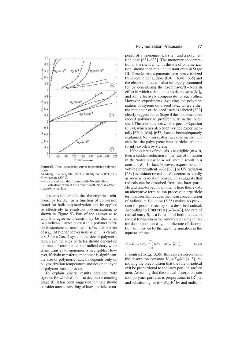
Polymerization Processes 77
Figure 53. Time – conversion curves for emulsion polymer-izationA) Methyl methacrylate (60 ◦C); B) Styrene (60 ◦C); C)Vinyl acetate (50 ◦C)—- calculated with the Trommsdorff–Norrish effect· · · · · calculated without the Trommsdorff–Norrish effect◦ experimental data
It seems remarkable that the empirical rela-tionships for Ktp as a function of conversionfound for bulk polymerization can be appliedso effectively to emulsion polymerization, asshown in Figure 53. Part of the answer as towhy this agreement exists may be that whentwo radicals cannot coexist in a polymer parti-cle (instantaneous termination), n is independentof Ktp. At higher conversions when n is clearly> 0.5 for a Case 2 system, the size of polymericradicals in the latex particles should depend onthe rates of termination and radical entry whenchain transfer to monomer is negligible. How-ever, if chain transfer to monomer is significant,the size of polymeric radicals depends only onpolymerization temperature and not on the typeof polymerization process.
To explain kinetic results obtained withstyrene, for which Rp fails to decline on enteringStage III, it has been suggested that one shouldconsider uneven swelling of latex particles com-
posed of a monomer-rich shell and a polymer-rich core [631–633]. The monomer concentra-tion in the shell, which is the site of polymeriza-tion, should then remain constant even in StageIII. These kinetic arguments have been criticizedby several other authors [630], [634], [635] andthe observed facts can also be largely accountedfor by considering the Trommsdorff – Norrisheffect in which a simultaneous decrease in [M]pand Ktp effectively compensate for each other.However, experiments involving the polymer-ization of styrene on a seed latex where eitherthe monomer or the seed latex is labeled [632]clearly suggest that in Stage II the monomer doesindeed polymerize preferentially in the outershell. The contradiction with respect to Equation(3.34), which has also been verified experimen-tally [620], [636], [637], has not been adequatelyexplained. Neutron scattering experiments indi-cate that the polystyrene latex particles are uni-formly swollen by styrene.
If the exit rate of radicals is negligible (m = 0),then a sudden reduction in the rate of initiationin the water phase to Ri = 0 should result in aconstant Rp. In fact, however, experiments in-volving intermittent γ-Co [638] or UV radiation[639] as initiator reveal that Rp decreases rapidlyas soon as irradiation ceases. This suggests thatradicals can be desorbed from one latex parti-cle and reabsorbed in another. There thus existsan alternative termination process: interparticletermination that reduces the mean concentrationof radicals n. Equation (3.35) makes no provi-sion for possible reentry of a desorbed radical.According to Ugelstad [640–643], the rate ofradical entry Ri is a function of both the rate ofradical formation in the aquous phease by initia-tor decomposition Ri, w and the rate of desorp-tion, diminished by the rate of termination in theaqueous phase:
Ri =Ri,w +Kd
∞∑
n=1
nNn−2Ktw [R·]2w (3.43)
In contrast to Eq. (3.35), this expression containsthe desorption constant Kd = K0S/v [s−1], re-moving the precondition that the rate of radicalexit be proportional to the latex particle surfacearea. Assuming that the radical absorption rate
into polymer particles is proportional to [R•
]Wand substituting for Ri = Ka [R
•
]W and multipli-

78 Polymerization Processes
cation by(
vKtpNp
)
and making the following
substitutions:
α=Ri v
KtpNp; α′=
Ri,w v
KtpNp;
m=Kd v
Ktp; Y =
2NpKtpKtW
K2a v
gives
α = α′+mn−Y α2 (3.44)
where Y is a dimensionless group.Equations (3.41) and (3.44) permit calcula-
tion of n as a function of a′, m, Y . The resultsfor Y = 0 (i.e., negligible termination in the waterphase) are shown in Figure 54. It is apparent thatthere is a rather large range of parameter values(α′ and m) for which n< 0.5; this is discussedfurther in [640] and [597, p. 559 ff].
Figure 54. Average number of radicals n per latex particle,assuming interparticle termination and a negligible amountof termination in the aqueous phase (Y = 0), calculated byusing Equations (3.41 and 3.44) [640]
The number of radicals in a polymer par-ticle clearly depends on rates of radical entry,desorption, bimolecular termination, and chaintransfer. Although radical capture efficiencies bypolymer particles can be high [644], efficienciesconsiderably below 100 % have been observed[645]. Brooks [644] has presented general ex-pressions for radical absorption rates which ac-count for reabsorption and give capture efficien-cies less than 100 %. Various experimental tech-niques for the measurement of desorption rateshave been employed [645–647]. Lichti et al.[648] obtained significantly enhanced desorp-tion rates from polystyrene particles containing
soluble hydrocarbon diluents. It has been sug-gested that in some systems desorbed radicalscross-terminate in the water phase and are not re-absorbed. Nomura et al. [649] used the pseudo-kinetic rate constant method to develop expres-sions forn for binary copolymerizations that fol-low the terminal model. Nomura et al. [650]also observed that the extent of Stage I (particlenucleation stage) could be lengthened by radicaldesorption.
Mechanism of Particle Formation. Asemulsion polymerization always involves a cer-tain amount of monomer in the aqueous phase,and for this reason all the routes depicted inFigure 55 represent possible reactions of theradicals or radical ions that form in the waterphase by initiator decomposition:
1) Entry into micelles, which are then trans-formed into latex particles
2) Propagation within the aqueous phase untila specific critical degree of polymerizationPcr is reached, at which point the growingmacroradical precipitates to form a latex par-ticle
3) Entry into an existing monomer droplet,which is converted into a latex particle
4) Entry into an existing latex particle, which isthen subject once again to propagation (seedpolymerization)
Figure 55. Possible radical reactions leading to particle for-mation during emulsion polymerization (schematic)
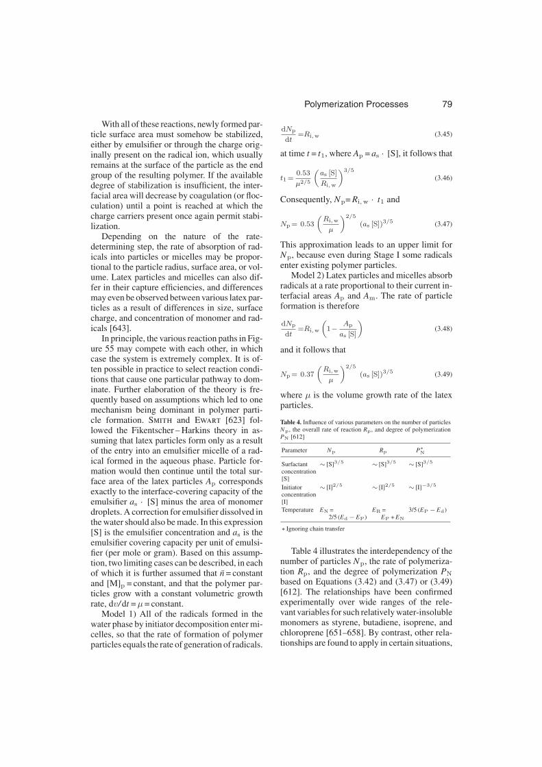
Polymerization Processes 79
With all of these reactions, newly formed par-ticle surface area must somehow be stabilized,either by emulsifier or through the charge orig-inally present on the radical ion, which usuallyremains at the surface of the particle as the endgroup of the resulting polymer. If the availabledegree of stabilization is insufficient, the inter-facial area will decrease by coagulation (or floc-culation) until a point is reached at which thecharge carriers present once again permit stabi-lization.
Depending on the nature of the rate-determining step, the rate of absorption of rad-icals into particles or micelles may be propor-tional to the particle radius, surface area, or vol-ume. Latex particles and micelles can also dif-fer in their capture efficiencies, and differencesmay even be observed between various latex par-ticles as a result of differences in size, surfacecharge, and concentration of monomer and rad-icals [643].
In principle, the various reaction paths in Fig-ure 55 may compete with each other, in whichcase the system is extremely complex. It is of-ten possible in practice to select reaction condi-tions that cause one particular pathway to dom-inate. Further elaboration of the theory is fre-quently based on assumptions which led to onemechanism being dominant in polymer parti-cle formation. Smith and Ewart [623] fol-lowed the Fikentscher – Harkins theory in as-suming that latex particles form only as a resultof the entry into an emulsifier micelle of a rad-ical formed in the aqueous phase. Particle for-mation would then continue until the total sur-face area of the latex particles Ap correspondsexactly to the interface-covering capacity of theemulsifier as · [S] minus the area of monomerdroplets. A correction for emulsifier dissolved inthe water should also be made. In this expression[S] is the emulsifier concentration and as is theemulsifier covering capacity per unit of emulsi-fier (per mole or gram). Based on this assump-tion, two limiting cases can be described, in eachof which it is further assumed that n = constantand [M]p = constant, and that the polymer par-ticles grow with a constant volumetric growthrate, dv/ dt =µ= constant.
Model 1) All of the radicals formed in thewater phase by initiator decomposition enter mi-celles, so that the rate of formation of polymerparticles equals the rate of generation of radicals.
dNp
dt=Ri,w (3.45)
at time t = t1, where Ap = as · [S], it follows that
t1 =0.53
µ2/5
(
as [S]
Ri,w
)3/5
(3.46)
Consequently, Np= Ri, w · t1 and
Np = 0.53
(
Ri,w
µ
)2/5
(as [S])3/5 (3.47)
This approximation leads to an upper limit forNp, because even during Stage I some radicalsenter existing polymer particles.
Model 2) Latex particles and micelles absorbradicals at a rate proportional to their current in-terfacial areas Ap and Am. The rate of particleformation is therefore
dNp
dt=Ri,w
(
1−Ap
as [S]
)
(3.48)
and it follows that
Np = 0.37
(
Ri,w
µ
)2/5
(as [S])3/5 (3.49)
where µ is the volume growth rate of the latexparticles.
Table 4. Influence of various parameters on the number of particles
Np, the overall rate of reaction Rp, and degree of polymerization
PN [612]
Parameter Np Rp P∗N
Surfactant
concentration
[S]
∼ [S]3/5∼ [S]3/5
∼ [S]3/5
Initiator
concentration
[I]
∼ [I]2/5∼ [I]2/5
∼ [I]−3/5
Temperature EN =
2/5 (Ed−EP)
ER =
EP + EN
3/5 (EP−Ed)
∗ Ignoring chain transfer
Table 4 illustrates the interdependency of thenumber of particles Np, the rate of polymeriza-tion Rp, and the degree of polymerization PN
based on Equations (3.42) and (3.47) or (3.49)[612]. The relationships have been confirmedexperimentally over wide ranges of the rele-vant variables for such relatively water-insolublemonomers as styrene, butadiene, isoprene, andchloroprene [651–658]. By contrast, other rela-tionships are found to apply in certain situations,

80 Polymerization Processes
especially in the case of more soluble monomerswith large transfer-to-monomer rate constants,including vinyl acetate and vinyl chloride [640],[642], [659–664]. Even in the case of styrene itis not possible to explain all the experimentalresults on the basis of the Smith – Ewart theory.If particle formation were to conform to Model1, then at the end of Stage I, each latex par-ticle would contain precisely one radical, i.e.,n = 1 [665]. In addition the molecular mass of thepolymer chain in a particle nucleated near t = 0would be extremely large at the end of Stage I.For Model 2, n = 0.67 at the end of Stage I [628].Since n = 0.5 during Stage II, Rp must peak atthe end of Stage I. However, no such maximumhas been observed with styrene. Moreover, Np
calculated by using Equations (3.47) or (3.49)often exceeds observed values by a factor of2 – 3. These discrepancies can be rationalized byassuming that latex particles are more efficientat capturing radicals than micelles [665], [666].Some particle coagulation would also reduce thediscrepancy. If radicals formed in the aqueousphase can enter either micelles or latex particles,the condition for radical balance assures that
d [R·]
dt=Ri,w−K1 [Mi] [R
·] −K2Np [R·] (3.50)
where [Mi] is the micelle concentration. Assum-ing a stationary state is valid, one obtains
[R·] =Ri,w
K1 [Mi] +K2Np(3.51)
Particle formation should only occur after theentry of a radical into a micelle, so
dNp
dt=K1 [Mi] [R
·] (3.52)
Substitution of Equation (3.51) into (3.52) gives
dNp
dt=
K1 [Mi]Ri,w
K1 [Mi] +K2Np=
Ri,w
1+K2Np
K1[Mi]
=Ri,w
1+εNp
[S]
(3.53)
where [S]/[Mi] = Mm is the aggregation numberfor emulsifier molecules in micelles (in manycases, Mm≈ 100); K2Np/K1 [M i] = εNp/[S] isthe ratio of the rate of entry into latex particlesversus micelles, and ε= (K2/K1)Mm character-izes the radical capture efficiency of latex parti-cles relative to micelles. For εNp/[S]≪ 1, Equa-tion (3.53) is equivalent to Equation (3.45) and
Smith – Ewart kinetics are applicable in the formof Equation (3.47).
On the other hand, in the case whereεNp/[S]≫ 1, there is a somewhat differ-
ent dependency, with Np∼ (Ri, w)2/7 and
Np∼ [S]5/7. To obtain agreement between cal-culated and experimental Np, it is necessary tointroduce the values ε= 1.3× 10⁵ for styrene[666] and ε= 1.2× 10⁷ for vinyl acetate [667].This is explained by assuming that radicals exitvery rapidly from very small latex particles aswell as micelles – so rapidly that they do not havesufficient time to propagate to the extent requiredfor insolubility in the water phase. Hansen andUgelstad [597, p. 556, 602 ff], [668] have ap-plied Danckwerts theory of diffusion with ho-mogeneous reaction [669] to this problem. Therate of absorption by latex particles that alreadycontain a radical is significantly larger than thatof latex particles and micelles containing no rad-icals, because the rate of termination betweentwo radicals is much higher than the rate of prop-agation. Termination by combination with a sec-ond radical normally leads to molecules that areno longer able to desorb due to having exceededthe critical degree of polymerization Pcr.
In the derivation of Equations (3.47) and(3.49) the volumetric growth rate µ of a latexparticle, given by
µ=dv
dt=
Kpϕm
NA (1+ϕm)·m
p·n (3.54)
was considered constant since n was taken to bea constant, independent of the latex particle age.This assumption is no longer valid when Case1 kinetics apply, and n increases with particlegrowth. Reference [643] has therefore adoptedthe following general relationship for the rate ofparticle formation:
dNp
dt=Ri ·
δNM rχM
δNM rχM +NM rχ
p(3.55)
where NM is the number of micelles, rM is themicelle radius, and rp is the particle radius, χ(= 1, 2, 3) is the exponent that characterizes thedependence of the capture rate on the radii of themicelles and polymer particles, and δ is an effi-ciency factor for the capture of radicals by mi-celles relative to polymer particles. This in turnis a function of the factor ε in Equation (3.56):
Polymerization Processes 81
δ=Mm
ε
(
rp
rM
)χ
(3.56)
Neglecting termination in the aqueous phase,Equation (3.43) is transformed into
Ri =Ri,w +Kd nNp (3.57)
and Equations (3.55) and (3.57) then lead to
dNp
dt=
Ri,w +KdnNp[
1+Np
δ NM
(
rp
rM
)x] (3.58)
Assuming that only monomer transfer radicalsare capable of desorbing from latex particles,Hansen and Ugelstad [643] constructed abalance equation for the formation and disap-pearance of latex particles containing a singlemonomer transfer radical, and then proceededto solve it under the assumption of steady state.One can then assume either that desorbed radi-cals do not add monomer in the aqueous phase,and instead simply wander from one particleto another, or that such radicals do in fact addat least one monomer molecule in the aqueousphase. In the latter case, no monomer transferradicals absorb into the latex particles, and thechain-transfer reaction becomes the sole sourceof monomer radicals in the particles. For furtherdetails refer to the original article [643]. Whatfinally results from these calculations is a setof curves representing the number of particlesNp as a function of the emulsifier concentration[S] and the rate of initiation Ri, w as shown inFigure 56 for various monomer types, assum-ing there is no chain transfer to monomer in theaqueous phase. Other graphs of interest corre-sponding to various values of δ and χ may befound in [643]. These curves serve as a basis forthe rule that the sum of the orders with respect to[S] or [I] (or Ri, w) for styrene, methyl methac-rylate, vinyl acetate, or vinyl chloride is alwaysin the vicinity of 1.0. Stated more generally
Np∼ [S]z ,Np∼ [I]1−z (3.59)
where 0.6< z< 1.0. If desorption and reabsorp-tion dominate (total radical entry rate≫Ri, w)z = 1.0; if there is no desorption of radicals,z = 0.6 (usual value for styrene). The actual valueof z may vary with [S] and [I]. If all other vari-ables are held constant, then an increase in [S]or [I] leads to an increase in the order z relative
to [S] or [I], while the order with respect to thevariable that is held constant decreases [643].
Figure 56. Number of particles Np as a function of A) theinitial emulsifier concentration [S]0 and B) the rate of initi-ation Ri, w for five different monomers [643] δ = 1.0; x = 1;
Ri, w in A = 1016 L−1 s−1 ; [S]0 in B = 1.0 g/Ldotted lines: Smith – Ewart theory (Eqs. 3.47 and 3.49)VAc: vinyl acetate; VC: vinyl chloride; MMA: methyl meth-acrylate; BMA: n-butyl methacrylate; S: styrene
In the case of monomers that are significantlymore soluble in water than styrene, it is also nec-essary to take into account the fact that latex par-ticles can be formed by homogeneous nucleationin the aqueous phase [655]. However, Equations(3.47) and (3.49) based on the Smith – Ewart the-ory (which, incidentally, do not explicitly refer toparticle formation from micelles) remain valideven when homogeneous nucleation is signifi-cant [670]. The rate of particle formation thenbecomes equal to either Ri, w (for Model 1 andEq. 3.47) or Ri, w minus the rate of radical cap-ture by previously formed latex particles (Model2 and Eq. 3.49). The volumetric growth rate µ istaken here to be constant, and particle nucle-ation ceases when the total latex particle surfacearea corresponds to as [S]. The concentration offree emulsifier should at this point be somewhatlower than the CMC.
Fitch and coworkers have developed the the-ory of homogeneous particle nucleation further[606, pp. 73 – 102, 103 – 116], [671–675]. With[S]<CMC, a radical produced in the aqueousphase by initiator decomposition continues togrow in this phase until it is either absorbed byan existing latex particle or a specific critical de-gree of polymerization Pcr has been exceeded,

82 Polymerization Processes
whereupon the macroradical precipitates andforms a primary polymer particle. In this casethe rate of particle formation is described by
dNp
dt=Ri,w − vc (3.60)
A steady-state (where Ri, w = vc) is reached att = ts, which means that the number of polymerparticles nucleated is given by
Np =
ts∫
0
(
Ri,w − vc)
dt (3.61)
originally, the rate of capture vc was taken to be
[628], [673].
vc =Ri,w
(
Npπr2)
L (3.62)
where L is the length of the path traversed by
the growing radical from its point of origin tothe point where it precipitates as a primary par-ticle (collision theory). This proposal has beensubjected to criticism [493, pp. 163 ff], [629] andthe expression
vc = 4πDopCSNpr (3.63)
where Dop is the mean diffusion coefficientfor oligomeric radicals and latex particles in theaqueous phase and CS is the concentration ofoligomeric radicals in the same phase in fact pro-vides a better fit than Equation (3.62) to exper-imental data on particle nucleation in the pres-ence of seed particle [675]. The effectivenessof seed particles in capturing oligomeric radi-cals before they grow and precipitate to formnew particles corresponds not to Npr2 but ratherto Npr. Hansen and Ugelstad [597, pp. 556,602 ff ], [643] have proposed a model for radicalcapture that takes into account not only the pos-sibility of radical desorption, but also the electro-static repulsion between radicals and particles.
One practical application of these considera-tions relates to stepwise seed polymerization asa means of preparing uniformly large (monodis-perse) latex particles [676], [677], in which thekey consideration is keeping vc as large as pos-sible; i.e., preventing the formation of new poly-mer particles.
Figure 57. Number of particles Np as a function ofconversion in the emulsion polymerization of methylmethacrylate with sodium dodecylsulfate as emulsifier[606, pp. 73 – 102]
Concentrations in mol/L: [S2O2−8 ] = 7.35× 10⁻⁴,
[HSO−3 ] = 1.14× 10⁻³ ; T = 30 ◦C
In certain formulations (e.g., in the absence ofemulsifier, or where the emulsifier concentrationis very low) charge density on the polymer par-ticle surface is insufficient to stabilize the result-ing particles. Moreover, with relatively solublemonomers such as methyl acrylate the interfa-cial tension is especially low, and emulsifiers areapparently less strongly adsorbed. The relation-ships here are further complicated by the factthat particles tend to coagulate until the surfacearea has been reduced (surface charge densityhas increased) sufficiently to restore stability, aprocess for which experimental evidence alsoexists [590, pp. 292 ff], [629], [678]. Figure 57shows experimental data for the production ofparticles by homogeneous nucleation, in whichmethyl methacrylate was polymerized with var-ious rates of initiation Ri, w and sodium dodecylsulfate concentrations ranging from zero to theCMC. With increasing conversion the numberof particles passes through a maximum beforefalling to a constant value. The conversion at thismaximum as well as the final constant number ofpolymer particles is lower for lower Ri, w valuesand lower emulsifier concentrations. Very sim-

Polymerization Processes 83
ilar results have been obtained with ethyl acry-late [679]. Electron micrographs of the resultingpolyacrylate latex particles after etching with O2
clearly show that they were formed by coagula-tion of a large number of smaller primary parti-cles.
If limited coagulation (or flocculation) oc-curs, it is necessary to also take into accountthe rate of flocculation vf , transforming Equa-tion (3.60) into
dNp
dt=Ri,w − vc − vf (3.64)
The Smoluchowski theory [680] can be used tocalculate the flocculation rate vf [674].
If to an anionic or cationic emulsifier there isadded a small amount of a straight-chain alco-hol whose chain length corresponds at least tothat of the emulsifier, then emulsification leadsto an especially stable emulsion consisting ofmany very small monomer droplets. Polymeri-zation of such an emulsion with an oil- or water-soluble initiator can, in an appropriate formula-tion, lead to almost total adsorption of the emul-sifier on the surface of the monomer droplets.Since the number of micelles is no longer largecompared to the number of monomer droplets,polymerization occurs partially or even princi-pally within the monomer droplets. The conse-quence is a bimodal distribution of polymer par-ticle sizes, where small particles formed in theaqueous phase are accompanied by large parti-cles whose origin is in the monomer droplets. Inthe limiting case, the size distribution of the la-tex particles corresponds almost exactly to thatof the original monomer droplet size distribution[681], [682]. These relatively large latex parti-cles may contain considerably more than oneradical and the observed polymerization kineticsare similar to those for homogeneous bulk poly-merization [683], [684]. This therefore repre-sents a transition toward suspension bead poly-merization.
An emulsion polymerization in which poly-merization occurs in both latex particles (formedfrom micellar or homogeneous nucleation) andmonomer droplets is called miniemulsion poly-merization (a term coined by the Lehigh Uni-versity Group). For such systems bimodal PSDas well as polymerization rates have been bothmeasured and predicted [685–687].
Song and Poehlein [688–690] have devel-oped new approaches to modeling homogeneousnucleation for monomers having a range of watersolubility. They account for the variation of thecritical chain length for precipitation with con-centration, and for sparingly soluble monomerssuggest that oligomers generated in the waterphase form micelles which are then stung by aradical to generate polymer particles. They alsoshowed that the number of polymer particles Np
increases slowly with emulsifier concentration[S] below the CMC, where homogeneous nu-cleation is dominant, but rapidly increases abovethe CMC due to micellar nucleation. Others haveconcluded that micellar nucleation is dominanteven for monomer with appreciable water solu-bility [691].
Radical scavengers (e.g., O2 and monomerinhibitors such as tert-butyl catechol) can haveinteresting effects on the number of polymer par-ticles formed and n. Radical scavengers havebeen classified as water soluble and monomer(organic) soluble [692], [693]. Oxygen, whichdissolves in water, monomer droplets, micelles,and polymer particles, mainly influences the ini-tiation of particle nucleation. Oxygen dissolvedin the aqueous phase reacts rapidly with primaryradicals, preventing particle nucleation. This re-sults in an induction period in which no poly-merization occurs. The induction period endswhen the oxygen content of the aqueous phasehas been reduced to an almost indetectable level.After the induction period, apart from usually aminor loss of initiator, the polymerization takesits normal course. However, in the presence of,say, tert-butyl catechol (an oil-soluble inhibitor)in the micelles and polymer particles, polymerparticles are nucleated, but n can be very lowdue to radicals reacting with inhibitor. This re-duces the volumetric growth rate µ and hencea larger number of polymer particles are nu-cleated (refer to Equations (3.47), (3.49), and(3.54). Once the organic-soluble inhibitor hasbeen consumed, the polymerization rate recov-ers but to a rate higher than originally expectedin the absence of the inhibitor. This phenomenoncan cause low-frequency oscillations in reactortrains when inhibitor contents in monomer recy-cle streams vary and potential safety problemsfor all reactor types (heat generation rate may beexcessive).

84 Polymerization Processes
3.3.3.4.2. Physicochemical Parameters ofDispersions
This section treats some properties of disper-sions that can be unambiguously described interms of physiochemical quantities. In additionto these, applications technology makes use ofa number of other characteristics, primarily em-pirical quantities and tests, [694], [695].
Molecular Mass Distribution of LinearHomopolymer Chains. In emulsion polymer-ization, chain transfer to monomer is more im-portant than in homogeneous bulk polymeriza-tion because bimolecular termination rates for agiven polymerization rate are generally lower foremulsion polymerization. This is why it is pos-sible to obtain high molecular mass at high poly-merization rates in these systems. When transferto monomer is dominant in controlling molec-ular mass development, the process type is ir-relevant and molecular masses of linear chainsdepend solely on polymerization temperature.Therefore, equations developed in Section 2.2for bulk and solution polymerization in homoge-neous media may be used to calculate molecularmass distributions. A useful experimental testto determine whether chain-transfer reactionsto small molecules (monomer or chain-transferagent) are dominant in producing polymer is tochange the concentration of initiator by severalfold. If molecular masses decrease with increas-ing initiator concentration then a significant frac-tion of polymer chains are formed by bimolec-ular termination. However, if polymer molecu-lar mass is independent of initiator concentra-tion, then chain-transfer reactions are dominantin producing polymer chains [696].
When termination reactions are significant inmolecular mass development, the calculation ofMWD and average molecular masses is gener-ally not straightforward. There are several com-plicating factors. Firstly, the MWD depends onthe polymer particle size distribution, which isdifficult to predict in commercial latex systems.Even if the PSD were known one would stillneed to know the mechanism by which radicalsenter particles. Attempts to predict the PSD havebeen made by using population balance methods[697–700].
Experimental verification of these PSD pre-dictions is lacking in most cases. The molecular
masses depend on radical entry rate per parti-cle, which in turn is some unknown function ofparticle size and number. For the special caseof a monodisperse latex the radical entry rateis known, however, and this case can be easilytreated when termination is instantaneous (rateof radical entry is much smaller than the rate oftermination in the polymer particle; or in otherwords two radicals cannot coexist in a poly-mer particle). This is true for Case 2 kinetics(n = 1/2). An expression is now derived whichdescribes molecular mass development for thisspecial case. Transfer to monomer and to chain-transfer agent are included in the analysis.
Consider an oligomeric radical in a polymerparticle. The probability that this radical adds r
monomer molecules and then terminates eitherby chain transfer to monomer or chain-transferagent T or by instantaneous termination with anew oligomeric radical which enters the particlefrom the aqueous phase is given by ϕr (1−ϕ),where
ϕ=Kp [M]p
Kp [M]p +Kfm [M]p +KfT [T]p +(
Ri,w
Np
)
NA
(3.65)
The instantaneous weight chain length distribu-tion W (r, t) is therefore given by
W (r, t)=r (1− ϕ) ϕr
0∫
∞
r (1−ϕ) ϕrdr
=r (1−ϕ)2 exp (− (1−ϕ) r) (3.66)
where K fm and K fT are rate constants for chaintransfer to monomer and chain-transfer agent T.
Equation (3.66) is the most probable distribu-tion, with number- and weight-average degreesof polymerization given by
PN =1
(1−ϕ)(3.67)
PW/PN = 2 (3.68)
These expressions should be valid for systemssuch as styrene and methyl methacrylate whenCase 2 kinetics apply and the PSD is quite nar-row. It is worth mentioning that in bulk polymer-ization of styrene at low conversions the poly-dispersity (PW/PN) is 1.5 because bimoleculartermination by combination produces most of
Polymerization Processes 85
the polymer chains. A polydispersity of 2 inemulsion polymerization is due to the fact thatwhen termination is instantaneous, terminationby combination acts like termination by dis-proportionation. In fact the polydispersity (forpolymer produced instantaneously) obtained inemulsion polymerization of any monomer typewill always be equal to or greater than that inhomogeneous solution or bulk polymerization.Equations (3.66) – (3.68) apply to an essentiallymonodisperse latex. For polydisperse PSD it isclear that instantaneous molecular mass proper-ties will be broader as will the MWD of polymeraccumulated in the polymer particles over poly-merization times of several hours. For most com-mercial recipes, chain-transfer agents are used tocontrol molecular mass development. In thesecases, the MWD is independent of the PSD,and molecular mass calculations for both poly-mer produced instantaneously and accumulatedpolymer are straightforward. ϕ is then equalto K fT [T]p/Kp [M]p, the instantaneous weightchain length distribution is again given by Equa-tion (3.66), and the MWD of the accumulatedpolymer for a batch reactor is given by Equation(3.69)
W (r, t)=
t∫
0
W (r, t) Rpdt
t∫
0
Rpdt
(3.69)
Several theoretical papers dealing with MWDdevelopment in emulsion homopolymerizationsare available [701–705]. The problem has nowbeen fully solved [706], [707] for the case whentwo or more radicals can coexist in a polymerparticle (zero – one – two, systems). When thePSD is broad, the population balance equationsfor particle size and molecular mass are cou-pled, requiring numerical solution of a large setof partial differential equations [708].
Polymer Chains with Long-Chain Branch-ing. Long-chain branching and cross-linkingcan occur as a result of chain transfer to polymerand by addition of polymeric radicals to termi-nal and pendant double bonds. The dimension-less groups which are relevant in polymer chainmodification by these reactions are
F1KfpQ1
Kp [M]p,K∗pQ0
Kp [M]pand
F2K∗pQ1
Kp [M]p
where K fp, K∗p are chain transfer to polymerrate constant and rate constant for the additionof polymeric radicals to terminal and pendantdouble bonds, respectively; Q1 is the number ofmoles per liter of monomer molecules chemi-cally bound to polymer chains (proportional tograms per liter of polymer); Q0 is moles of poly-mer per litre which have a terminal double bond;F1 is the fraction of monomer molecules in thepolymer chains which have an extractable atom;F2 is the fraction of monomer molecules in thepolymer chains which have a pendant doublebond. As these dimensionless groups increasein value, long-chain branching and cross-linking(cross-linking density and gel/sol ratio) increase.These groups increase with monomer conver-sion and usually increase with polymerizationtemperature. Long-chain branching and cross-linking reactions are more important in emul-sion polymerization than in homogeneous so-lution, bulk, and suspension polymerization be-cause even at the birth of a latex polymer particle,the concentration of polymer in the particle islarge [709]. Chain branching, cross-linking, andgel formation are undesirable for the manufac-ture of cold SBR and NBR by continuous emul-sion polymerization. To minimize long-chainbranching, three important features of plant de-sign are:
1) A large number of back-mixed reactors in se-ries (this gives a narrow residence-time dis-tribution which is desirable for low levels ofbranching)
2) The final conversion is kept rather low (ca.63 % monomer conversion for cold SBR)
3) The polymerization temperature (ca. 5 ◦C forcold SBR) is kept low to reduce K fp/Kp andK∗p/Kp
When carrying out semi-batch emulsionpolymerization, extending the addition time ofmonomers lowers [M]p, and this can lead tohigher levels of long-chain branching and cross-linking.
Linear and Branched Copolymer Chains.For such calculations, it is recommended thatthe pseudo-kinetic rate constant method be em-ployed. Emulsion copolymerizations can be suc-cessfully modeled (calculations of polymeriza-tion rate, chain microstructure, molecular mass,
86 Polymerization Processes
and long-chain branching and cross-linking) byapplication of the pseudo-kinetic rate constantmethod [417], [649], [710] and properly ac-counting for changes in chemical and physicalproperties during the course of polymerization[711–713].
Copolymer composition is usually control-ling semi-batch operation [357], [405], [714],[715]. The composition of polymer particles de-pends on the thermodynamic compatibility ofpolymer chains and is not always spatially uni-form. Core/shell morphology, which is oftenthe planned particle morphology for specialtyproducts, can be effected by grafting and cross-linking reactions as well as compositional drift[715–718]. Special end use properties can be ob-tained by controlling morphology [719], [720].The morphology of latex particles is also a func-tion of the mechanism of particle formation.Limited coagulation (flocculation) leads to latexparticles composed of a number of not entirelyfused smaller primary particles. Such particlesare often not smooth and spherical, displaying arather rough surface and an irregular lumpy or“potato-like” shape [721].
Polymer Particle Size Distribution. Ingeneral, the PSD is narrower the lower theconversion at the end of Stage 1 is relativeto the final conversion at the end of the poly-merization. In the limiting case of stepwise seedpolymerization, no new polymer particles areproduced, even though a very high monomerconversion is reached, resulting in larger latexparticles that are nearly monodisperse in PSD[676], [677]. A semiquantitative calculation[590, p. 275 ff] based on Smith – Ewart Case 2kinetics shows that PSD narrows with increasingmonomer/water ratio, as well as with increasingtemperature, increasing initiator concentrationin the aqueous phase, and decreasing emul-sifier concentration [S]. Experiments involvingstyrene have confirmed these predictions. Quan-titative calculations are also in good agreementwith experiment [606, pp. 153 – 161] for styreneemulsion polymerization. A more comprehen-sive population balance model which accountsfor coagulation in the seeded emulsion poly-merization of vinyl chloride has been developed[722]. The predicted bimodal distributions ofparticle size are in good agreement with experi-mental data.
Gianetti [699] in a theoretical study of theevolution of PSD in Stage 2 has reviewed themore important theoretical studies and discussedtheir limitations. The results obtained representa generalization of previous theories in that
1) A comprehensive description for monomersystems which conform to zero – one kinet-ics has been made
2) The contribution of latex particles havingmore than one growing radical has beenproperly accounted for
3) Bimolecular termination has been explicitlyincluded in the model (at least where mutualannihilation of two growing chains is not themain termination reaction)
4) General expressions for the time evolutionof the cumulants of the PSDs (both in thetransient and nontransient case) have beendetermined
Gianetti’s solutions not only revise theoret-ical misinterpretations which appeared in the lit-erature, but also allow rate coefficients to be ex-tracted with more precision from reliable experi-mental data. In this connection it has been shownthat rate coefficients obtained from experimen-tal PSD data are in good agreement with val-ues found by using dilatometry to measure ratesof polymerization. Recent interest in analyzingthe experimental time evolution of PSD is duemainly to the possibility of determining kineticrate constants with a small confidence interval[602], [723]. According to Gianetti’s solutionsPSD and kinetic data are not independent of eachother at steady state (in other words, if a certainvolume dependence for the entry rate constant isassumed, from the analysis of an experimentalPSD one must find the same volume dependencefor the exit rate constant). Apparently, PSDs forsystems with n≤ 1/2 are insensitive to assump-tions about the mechanisms of radical entry andexit. In this connection, a new approach based onthe effect of PSD on MDW has been proposed[724]. In fact, a similar approach was proposedmuch earlier by DeGraff and Poehlein [725].A CSTR was used to obtain a broad PSD forstyrene emulsion polymerization, and assumingthat radical capture was according to the colli-sion theory (capture rate∼ r2), a polydispersityof 4.84 was calculated for the MWD, DeGraff
and Poehlein’s MWD measurements showedthat the molecular mass averages MN and MW
Polymerization Processes 87
were independent of mean residence time andthat the polydispersity was ca. 3. The discrep-ancy between theory and experiment may be dueto any number of possibilities, including:
1) Perhaps the collision model is not valid (trythe diffusion model)
2) Larger latex particles may not obey Case 2kinetics
3) Transfer to monomer may not be insignifi-cant
Similar experimental data were found forcontinuous emulsion polymerization of styrenein a CSTR [726]. Simultaneous growth of la-tex particles by polymerization and coagulationmay occur at various stages in emulsion poly-merization [688–690], [723], [727–730]. For thecalculation of PSD in the emulsion polymeriza-tion of vinyl chloride, it may be necessary toaccount for coagulation [731], [732].
The extent of coverage of the particle sur-faces by emulsifier is an important factor in thestability of a dispersion. For example, this cover-age should not be too large if the polymer is to belater recovered by controlled coagulation. Thesurface coverage is evaluated in a detergent titra-tion [733], [734], in which the amount of emul-sifier that must be added to give total monomo-lecular coverage of the surface is measured. To-tal coverage is indicated, for example, by thepoint where additional emulsifier no longer low-ers the surface tension (surface tension remainsconstant after micelles are formed). If the sur-face coverage required for particle stability isknown, emulsifier can be added during Stage IIto maintain stability but not form new micelleswith the danger of nucleating a second family ofparticles. More is involved here than simply theadsorption of an emulsifier on the particle sur-faces, however. The majority of the hydrophilicend groups on polymer molecules also tend tomigrate to the interface (e.g., – OH, – SO4, –COOH), thereby contributing to stabilization ofthe polymer particles. A comparable effect isachieved by the addition of small amounts ofhydrophilic comonomers (e.g., acrylic or meth-acrylic acid), which polymerize preferentially atthe particle surface [721].
The minimum film-forming temperatureof a polymer is the lowest temperature at which
a dispersion can be converted into an integralfilm on a surface by evaporation of the water.This normally corresponds approximately to theglass transition temperature Tg of the polymerand is one of the most important application pa-rameters of a polymer dispersion. Copolymer-ization of monomers whose homopolymers havea range of glass transition temperatures makesit possible to achieve desired values for boththe glass temperature and the minimum film-forming temperature. The glass transition tem-perature [Tg] of the copolymer can be calculatedby using the equation
Tg =W1Tg1 +KW2Tg2
W1 +KW2withK=
∆α1
∆α2(3.70)
where W1 and W2 are mass fractions ofmonomers 1 and 2 in the copolymer, Tg1 and Tg2
are the glass transition temperatures of the cor-responding homopolymers, and ∆α1 and ∆α2
are the differences between the thermal expan-sion coefficients above and below Tg (melt andglass) for the two homopolymers.
3.3.3.4.3. Inverse Emulsion Polymerization
In inverse emulsion polymerization, a hy-drophilic monomer is dissolved in water, emulsi-fied in a continuous hydrophobic oil phase witha water-in-oil emulsifier, and polymerized by us-ing an oil- or water-soluble initiator. The productis a latex consisting of very small polymer par-ticles, swollen with water and suspended in anoil continuous phase. The emulsified monomerdroplets are also very small, and they may serveas the source of some of the latex particles(a form of miniemulsion polymerization). Theoverall rate of polymerization is significantlyhigher here than in the corresponding solutionpolymerization. This observation strongly sup-ports the idea that what is occurring is a trueinverse emulsion polymerization rather than aninverse suspension polymerization. When oil-soluble initiators are used with aromatic con-tinuous phases the kinetics have been shownto resemble those of emulsion polymerization[576], [577], [735] with the locus of nucleationof particles in inverse micelles. However, whenparaffinic oil continuous phases are used, as ismost common commercially, the locus of par-ticle nucleation and polymerization is in the

88 Polymerization Processes
monomer droplets and the process is properlycalled inverse suspension polymerization (theterm microsuspension is often used because themonomer droplets are nominally 1 µm in diam-eter) [575]. This has been verified by dynamiclight scattering measurements which failed todetect inverse micelles and indicated a con-stant particle size throughout the polymeriza-tion [578–580]. Reviews of polymerization ininverse emulsions and microemulsions are avail-able [736–738]. Inverse microsuspension poly-merization has been used to study the kineticsof polymerization of acrylamide with cationiccomonomers (quaternary ammonium cationicmonomers) [739].
Water-in-oil emulsions of high molecularmass polyacrylamide and acrylamide copoly-mers (anionic and cationic) are particularly use-ful as flocculating agents in sewage treatmentand as retention aids in papermaking. At thepresent time inverse emulsion and microsuspen-sion polymerization is the only technology forthe large-scale production of very high molec-ular mass polymers in a liquid-like form thataffords a convenient suspension viscosity, highsolids content, and easy phase inversion duringapplication [740–742].
3.3.3.4.4. Semi-Batch EmulsionPolymerization
In semi-batch polymerizations, water,monomers, initiators, and emulsifiers may beadded to a reactor over a time period whichis comparable to the total polymerization time(usually over several hours). Several feed poli-cies have been employed. For example, a startingmixture of water, emulsifier, and initiator is firstprepared, usually also containing a portion ofthe monomer; the remaining monomer (often to-gether with initiator) is added during the courseof polymerization (monomer feed) [743]. Withanother procedure, the polymerization is begunin a portion of the total batch, the rest beingfed into the reactor gradually after the onset ofpolymerization in the form of a monomer emul-sion (emulsion feed), although the compositionof the feed may well differ somewhat from thematerial used to initiate the process [744].
Semi-batch processes are intermediate bet-ween batch and continuous polymerization pro-
cesses. A monomer-feed process based on avery large starter mix resembles more batch pro-cesses, whereas an emulsion semi-batch processinvolving a small initial charge with most of themonomers being fed in during the semi-batchperiod is more similar to continuous processes.These two semi-batch methods are often men-tioned in the patent literature [745]. Their advan-tages include better control of polymerizationand heat-generation rates by appropriate manip-ulation of feed rates. Moreover, the concentra-tion of unreacted monomer can be minimized(offering a safer process which is less prone torunaway) and cold feed can give higher produc-tivity (less demand for jacket or condenser cool-ing, for example). In the case of copolymeriza-tions, it is possible to manipulate monomer feedsto control copolymer composition [746–751]. Inparticular, such methods are often exploited forthe purpose of reaching a specific degree of poly-merization, particle size, or particle size distri-bution without changing the overall compositionof the copolymer in the latex particles. Adjust-ment of the process parameters can also havean influence, for example, on the stability of anacrylate dispersion [752–755].
Kinetic studies [756], [757] have shown that,provided the feed rate is not too large, bothtypes of semi-batch polymerization experiencea quasi-steady state in which the polymeriza-tion rate and feed rate of monomer remain com-parable. During the semi-batch feeding period,the concentration of monomer [M]p is rela-tively constant and it stays below the satura-tion concentration predicted by Equation (3.34).The resulting conversion – time curves are lin-ear over a wide range of monomer feed times.Increasing the monomer feed rate causes an in-crease in [M]p and according to Equation (3.42)this also leads to increases in both Rp and PN.Slower feed rates prolong the steady state pe-riod, and this should result in a narrower MWDfor the polymeric product [757], [758]. Prolong-ing the monomer feed period lowers [M]p andraises polymer concentration. For certain typesof monomer this can lead to greater long-chainbranching and cross-linking [355], [357].
When every ingredient except a reserve por-tion of the monomer is initially charged to thereactor, the phase ratio of monomer/water differsfrom the corresponding batch process, but thishas no effect on the number of particles nucle-

Polymerization Processes 89
ated. On the other hand, when polymerization isinitiated in a portion of the complete recipe, thenumber of polymer particles nucleated per unitvolume of emulsion may not be the same as fora batch process. Clearly the number of particlesnucleated in the initial charge will be much less.If the onset of addition is delayed until sometime after polymerization has begun, then StageI (the nucleation stage) for the initial charge mayhave been completed. If no further particles arenucleated during the semi-batch feed period, thefeed will be entirely directed towards the growthand stabilization of the existing polymer parti-cles. The number of polymer particles is thenfewer and their size at the end of the polymer-ization is larger. Based on the same total recipe,the two semi-batch processes just described canbe compared and contrasted as follows:
When the initial charge and the semi-batchfeed have the same recipe (composition), fewer(hence larger) latex particles are produced thanfor the batch process or the semi-batch processwith just monomer fed to the reactor over time.If particle formation is avoided during the semi-batch period, then the initial rate of polymeriza-tion Rp, o and the number of particles nucleatedNp will be proportional to the size of the initialcharge.
Assuming particle formation does not oc-cur during the semi-batch feed period, emulsionfeed provides a narrower PSD than monomerfeed or batch polymerization. If particle for-mation does occur during emulsion feed, thenthe PSD becomes broader, and in extreme casesit can be even broader than with the otherprocesses. Particle formation during semi-batchfeed can be suppressed by using a larger amountof initial charge and prolonging the time periodbefore semi-batch feed is initiated (i.e., morepolymer particles are nucleated and grow largerbefore semi-batch feed is initiated). Taking theincreasing surface area into account also makesit possible to adjust the emulsifier feed so thatnew polymer particles are not nucleated and nocoagulation occurs [759].
As long as the rate of addition of monomer issufficiently large to keep the polymer particlessaturated, then the rate and degree of polymer-ization for both semi-batch processes are inde-pendent of feed rate.
If the monomer concentration falls below itssaturation value in the polymer particles (due
to slow monomer feed, for example) then therate of polymerization will equal the monomerfeed rate. The rate of polymerization and heat-generation rate will increase with increasingmonomer feed rate. The polymerization temper-ature can therefore be controlled by manipulat-ing the monomer feed rate.
For the control of copolymer compositiondistribution, various monomer feed policies maybe used and equations have been developed todetermine the appropriate time-dependent feedrates required [356], [357], [405]. Considerationof molecular mass, long-chain branching, andcross-linking is also possible [357].
3.3.3.4.5. Continuous EmulsionPolymerization
Continuous emulsion polymerization is usedparticularly where the latex is to be coagu-lated and the solid polymer recovered. Im-portant examples include the manufacture ofstyrene – butadiene rubber (cold SBR) [760–762], acrylonitrile – butadiene rubber (NBR)[763], polychloroprene [764], [765], SAN andABS polymers [766–769], and poly(vinyl chlo-ride) [733], [770]. For products used in latexform, most manufacturers prefer the flexibilityassociated with batch and semi-batch processes,especially with product lines that are subject tofrequent change. Apparently, however, there isalso a certain amount of large-scale polymer dis-persion manufacture by the continuous process.
Systematic investigations have been carriedout on the kinetics and mechanisms of par-ticle formation in continuous stirred-tank orstirred-cascade reactors for styrene [771–781],styrene – butadiene [782], [418], [419], ethylene[783], vinyl chloride [733], [784], [785], vinylacetate [786–791], methyl methacrylate [786],and methyl acrylate [776]. A tubular reactor hasalso been analyzed [780] and review articles areavailable [792], [793] on the general subject ofcontinuous emulsion polymerization.
The most important elements of the theoryof emulsion polymerization in a stirred reac-tor or stirred reactor cascade have been pre-sented by Gerhsberg and Longfield [771].They began with the Smith – Ewart assumptionthat latex particles originate with the entry ofan oligomeric radical into a micelle, and that
90 Polymerization Processes
radicals enter both latex particles and micellesaccording to their surface areas (collision the-ory, with no distinction between micelles andpolymer particles). The following equation thendescribes the steady state with particle formationrate equal particle outflow rate (Case 2 kineticsapply)
dNp
dt=Ri,wAm
Am +Ap−Np
τ= 0 (3.71)
where Am and Ap are the surface areas per unitvolume of latex for micelles and polymer parti-cles and τ is the mean residence time of a singleCSTR. The residence-time distribution for latexparticles in a CSTR is given by
E (t) dt=dNp
Np=
1
τexp (− t/τ) dt (3.72)
where E (t) dt is the fraction of latex particles inthe exit stream with age t. Because latex particlesare very small and have a density close to that ofwater, the continuous phase, it is reasonable toassume that the residence-time distribution of la-tex particles and the aqueous phase are the same(latex particles follow streamlines).
It is further assumed that the role of molecu-larly dissolved emulsifier in the aqueous phasecan be neglected relative to the amount of emul-sifier in micelles and adsorbed on latex particles.Additional assumptions are that [S]≫CMC andthat
as [S] NA =Am +Ap (3.73)
The number of particles is then given by
Np =Ri,w τ
(1+Ap/Am)(3.74)
The particle surface area Ap for spherical lat-exparticles with various ages and sizes thus be-comes
Ap = 4.85
N∫
0
v2/3 dNp (3.75)
Substitution of v = f (Kp, t, [M]p, n) into Equa-tion (3.75), where [M]p is constant (due to thevery rapid diffusion of monomer from monomerdroplets to polymer particles and, if monomerdroplets are absent, due to rapid diffusion ofmonomer from polymer particle to polymer par-ticle; the direction of monomer diffusion should
be towards older and larger polymer particles)and n = 0.5 and combination with Equations(3.72) and (3.74) then gives
Np=Ri,wτ
[
1+KlRi,w τ
as[s]
(
Kpτ [M]pl−K2[M]p
)] (3.76)
As can be seen the comparison of Equations(3.74) and (3.76), the second term in the de-nominator of Equation (3.76) is analogous to thequantity Ap/Am. At low concentrations of emul-sifier [S] and high values of Ri, w and τ , it canbe assumed that Ap/Am≫ 1, so Equation (3.76)takes on the simplified form
Np =as
K1
[S]
(Kpτ)2/3
(
1−K2 [M]p
[M]p
)2/3
(3.77)
Substitution into Equation (3.42) then gives
Rp =K3 [M]pas [S] K
1/3p
τ2/3
(
1−K2 [M]p
[M]p
)2/3
(3.78)
Here the constants K1–K3 are functions of thespecific volumes Vm and Vp of monomer andpolymer as well as of the molecular masses ofthe monomers; K1 and K3 contain in addition theassumed constant n = 0.5 within the latex parti-cles [771].
In order to compare exprimental data ob-tained over a wide range of conditions, it is con-venient to rewrite Equation (3.76) in dimension-less form [772]:
(
Ri,wτ
Np
)
= 1+K1Ri,wτ
as [S]
(
τKp [M]p
1−K2 [M]p
)2/3
(3.79)
or
π1 = 1+π2
If Np is expressed in terms of Equation (3.42)and introduced into Equation (3.79), what resultsis a second dimensionless equation for Rp:
Ri,wτKp [M]p n
RpNA= 1+K1
Ri,wτ
as [S]
(
τKp [M]p
1−K2 [M]p
)2/3
(3.80)
or
π3 = 1+π2
Comparisons of data supplied by three differ-ent authors [771], [772], [776] are presented in

Polymerization Processes 91
Figures 58 A and 58 B. In Figure 58 A, essen-tially all of the points lie above the 45◦ line;that is, fewer latex particles are formed thanpredicted by theory. By contrast, the experi-mental values for Rp in Figure 58 B, which aremore precise, correspond well to the theoreticalstraight line. Overall, one may conclude that inthe case of styrene the theory is well substanti-ated. The Gershberg – Longfield theory has beenextended and modified a number of times. ThusDeGraff and Poehlein dropped the assump-tion that n = 0.5 and instead calculated n usingthe Stockmayer – O’Toole solution for differentparticle sizes (Eq. 3.41) [772]. This accounts forthe possibility of more than one radical per par-ticle for the larger particles. Nomura et al. [773]also applied Equation (3.53), according to whichradicals are absorbed more rapidly into latex par-ticles than into micelles, to continuous emulsionpolymerization and obtained a prediction that isin better agreement with experiment (as com-pared to that in Fig. 58 A). Brooks [794] dis-cusses various equations for the entry of rad-icals into latex particles and micelles, assum-ing among other things that micelles disintegrateonly slowly under subsaturation conditions, andthat even in the presence of micelles the surfaceof the latex particle may not be saturated withemulsifier.
Figure 58. A) Number of particles according to Equation(3.79), and B) Overall rate of polymerization according toEquation (3.80) for the continuous emulsion polymeriza-tion of styrene (dimensionless representation) [772]2 from [772]H from [771]◦ from [776]• calculated from values for Rp with the assumption thatn = 1/2
The existence of multiple steady states forthe isothermal operation of a CSTR was firstdemonstrated in the case of continuous emulsionpolymerization by Gerrens et al. [776–778], al-
though it had earlier been predicted on theoret-ical grounds for autocatalytic processes in gen-eral [795–806]. Autocatalytic acceleration hereis a consequence of the Trommsdorff –Norrisheffect. The mass balance for monomer at steadystate is given by
v [M]0 − v [M] −RpV = 0 (3.81)
where υ is the volumetric flow rate to and fromthe reactor, [M]o is the monomer concentrationin the feed, [M] is the monomer concentrationin the reactor and exit stream, V is the volume ofthe reacting mass in the reactor, and Rp is the rateof polymerization in the reactor. Furthermore,
1
τ
(
[M]0 − [M])
=Rp (3.82)
where τ = V /υ is the mean residence time in thereactor.
Figure 59 shows a graphical solution of Equa-tion (3.82) and Rp versus monomer concen-tration, in which data have been plotted as afunction of both monomer concentration [M]and conversion X. At low values of mean res-idence time τ , there is one intersection (one so-lution) between experimental Rp = f ([M]) andthe straight line (Eq. 3.82) which implies a singlestable operating point at low conversion. By con-trast, longer residence times lead to three pointsof intersection, with stable operating points atboth low and high conversions and an unsta-ble operating point at an intermediate conver-sion. For a train or cascade of n stirred reactorsthere may be as many as n + n (n + 1)/2 stableoperating points and n unstable operating pointsfor the individual reactors as well as n + 1 sta-ble states for the entire cascade. Oscillations inthe number of particles, the polymerization rate,and the interfacial tension have attracted consid-erable theoretical attention. These are attributedto bursts of particle formation that accompanyswings between states of supersaturation of thelatex particle surfaces, indicating large amountsof free emulsifier (and micelles), and states char-acterized by undersaturation, in which particleformation almost ceases. This phenomenon haslong been recognized in industrial-scale con-tinuous emulsion polymerization [733] and hasnow been thoroughly investigated in the case ofstyrene [771], [778], methyl methacrylate [786],[807], [808], and vinyl acetate [786], [798],[799], [809].
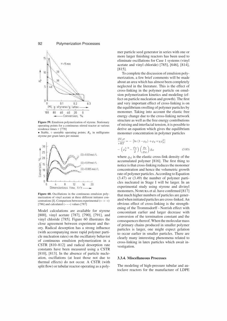
92 Polymerization Processes
Figure 59. Emulsion polymerization of styrene. Stationaryoperating points for a continuous stirred reactor at variousresidence times τ [778]• Stable, ◦ unstable operating points; Rp in milligramsstyrene per gram latex per minute
Figure 60. Oscillations in the continuous emulsion poly-merization of vinyl acetate at three different initiator con-centrations [I]. Comparison between experimental (◦ ·◦ ·◦)[786] and calculated (– – –) values [787]
Model calculations are available for styrene[800], vinyl acetate [787], [790], [791], andvinyl chloride [785]. Figure 60 illustrates theclose agreement between experiment and the-ory. Radical desorption has a strong influence(with accompanying more rapid polymer parti-cle nucleation rates) on the oscillatory behaviorof continuous emulsion polymerization in aCSTR [810–812] and radical desorption rateconstants have been measured using a CSTR[810], [813]. In the absence of particle nucle-ation, oscillations (at least those not due tothermal effects) do not occur. A CSTR (withsplit flow) or tubular reactor operating as a poly-
mer particle seed generator in series with one ormore larger finishing reactors has been used toeliminate oscillations for Case 1 systems (vinylacetate and vinyl chloride) [785], [646], [814],[815].
To complete the discussion of emulsion poly-merization, a few brief comments will be madeabout an area which has almost been completelyneglected in the literature. This is the effect ofcross-linking in the polymer particle on emul-sion polymerization kinetics and modeling (ef-fect on particle nucleation and growth). The firstand very important effect of cross-linking is onthe equilibrium swelling of polymer particles bymonomer. Taking into account the elastic freeenergy change due to the cross-linking networkstructure as well as the free energy contributionsof mixing and interfacial tension, it is possible toderive an equation which gives the equilibriummonomer concentration in polymer particles
2V1σ
rRT= −
[
ln (1−ϕp) +ϕp +χϕ2p
]
−(
ϕ1/3p −
ϕp
2
)
(
p
M
)
¯el (3.83)
where el is the elastic cross-link density of theaccumulated polymer [816]. The first thing tonotice is that cross-linking reduces the monomerconcentration and hence the volumetric growthrate of polymer particles. According to Equation(3.47) or (3.49) the number of polymer parti-cles nucleated in Stage I will be larger. In anexperimental study using styrene and divinylmonomers, Nomura et al. have confirmed [817]that much higher numbers of particles are gener-ated when initiated particles are cross-linked. Anobvious effect of cross-linking is the strength-ening of the Trommsdorff – Norrish effect withconcomitant earlier and larger decrease withconversion of the termination constant and theconsequences thereof. When the molecular massof primary chains produced in smaller polymerparticles is larger, one might expect gelationto occur earlier in smaller particles. There areclearly many interesting phenomena related tocross-linking in latex particles which await in-vestigation.
3.3.4. Miscellaneous Processes
The modeling of high-pressure tubular and au-toclave reactors for the manufacture of LDPE
Polymerization Processes 93
has received a great deal of attention [818–836].These models are notable for the detailed kinet-ics, which include transfer to polymer, backbit-ing, and β-scission in an attempt to calculateboth short- and long-chain branching frequen-cies. The polymerizations are almost adiabatic,with large temperature increases, and phase sep-aration between ethylene and polyethylene mayoccur in autoclave reactors. The tubular reactoris considered to be in plug flow, while mixingin the autoclave is rather complex and variousmixing models have been considered. A com-prehensive copolymerization model for ethyleneand comonomers in a high-pressure continuoustubular reactor has been developed [836].
A comprehensive tubular reactor model forthe solution polymerization of vinyl acetate hasbeen developed by Hamer and Ray [837]. Thekinetics employed account for transfer to poly-mer and reaction with terminal double bonds(trifunctional branching frequencies are calcu-lated). The model solves the equations of mo-tion for both axial and radial velocity profiles.Experimental validation of the model has beencarried out.
The bulk and solution polymerization ofstyrene in tubular reactors has also been exten-sively studied both theoretically and experimen-tally [375], [838]. Spatial distributions of veloc-ity, temperature, and concentration were mod-eled [838] and it was shown that for tube diame-ters > 2 cm, thermal runaway may occur. Inter-nal mixers were used in larger diameter tubesto give better radial mixing and this techniqueappears to give polystyrenes with high molecu-lar mass at a productivity of commercial interest[375]. References to other important studies onstyrene production in tubular reactors may befound elsewhere [375], [838].
Chemical Modification of Polymers in Ex-truders The commercial incentive for the chem-ical modification of polymers by chain scission,long-chain branching, cross-linking, and graft-ing is the enhancement of the physical and chem-ical properties of polymers and polymer mix-tures (alloys, blends, additives) and/or improve-ment of their processability. In many cases, theextruder has been found to be an effective chem-ical reactor in which chemical modification ofhigh molecular mass polymers in the melt canbe done economically for low-volume products.
It is particularly effective for chemical modi-fication of high molecular mass, solvent-free,commodity polymers to tailor-made productsto meet the growing diversity in polymer ap-plications. The extruder reactor provides shortand controlled residence times; efficient mix-ing, particularly for reactants at low concentra-tions; and good heat transfer. Multistage reac-tion, with sequential feeding of reactants andremoval of byproducts, is possible. There arecertain advantages of twin-screw over single-screw extruders [839]. These include: intenseshear mixing (with better surface renewal rates)giving molecular-level mixing (micromixing),improved heat transfer, multistage feeding, vent-ing of volatile byproducts, and screw speed canbe changed without changing the throughput.These attributes of the twin-screw extruders areideal for chemical modification where a smallamount of the low molecular mass compound tobe grafted on the polymer chains must be ho-mogeneously mixed with a highly viscous basepolymer.
Chemical modifications are often carried outusing free-radical reactions in the temperaturerange 170 ◦C – 350 ◦C. When a polymer con-taining a peroxide and a compound to be graftedis melt processed, chain scission, long-chainbranching, cross-linking, and grafting reactionsmay occur simultaneously. To optimize productproperties, the rates of these reactions must becontrolled.
Chain Scission. Polymer chain scission oc-curs when chemical bonds (usually C – C) alongthe backbone break. Since a higher molecu-lar mass chain has a greater number of suchbonds, it experiences chain scission preferen-tially (for polypropylene, scission seems to berandom with respect to the position of the bondalong the chain backbone [840], [841]). There-fore, the broad MWDs, usually found for poly-olefins narrow as the average molecular massfalls. With random scission occurring exclu-sively, the limiting polydispersity for all initialMWDs is two and the limiting MWD is Flory’smost-probable distribution. A reduction in mo-lecular mass improves processability. The out-standing commercial example of the use of con-trolled chain scission of polypropylene (PP) is inthe production of controlled-rheology PP usedfor fiber manufacture, film-extrusion, and forfast molding applications [842].
94 Polymerization Processes
Long-Chain Branching and Cross-Linking.
Long-chain branches (tetrafunctional) areformed when radical centers on the backbone ofpolymer chains experience bimolecular termina-tion by combination. If this long-chain branch-ing process continues, a three-dimensional net-work (cross-linked gel) is formed. The pro-duction of higher molecular mass chains bylong-chain branching produces a polymer thatexhibits increased die swell and melt strength,and improved strain-hardening properties [842].
Cross-linking of polymer chains results whenbimolecular coupling (via bimolecular termina-tion by combination of polymer backbone rad-icals or the reaction of grafted chemical groupssuch as those with silane functionality [843],[844]) of polymer chains to form tetrafunc-tional branches occurs repeatedly. The cross-linked polymer is a mixture of polymeric gel,of effectively infinite molecular mass, and solwhich is made up of linear and branched chains.Property enhancement due to cross-linking in-cludes: increased service temperature, solventresistance, flexural modulus, low-temperatureimpact strength, environmental stress crackingresistance, and reduced creep [842].
Grafting onto polymer chains can occurwhen a mixture of the polymer, peroxide, andunsaturated or saturated compound to be graftedare melt processed in an extruder. For exam-ple, acrylic acid or maleic anhydride can begrafted onto PP or PE to enhance compatabil-ity with more polar blends or to improve adhe-sion to metals, glass fibers, and to other polymertypes [845], [846]. Vinyl silanes can be graftedto polyolefins to subsequently produce cross-links in the presence of moisture [843]. Func-tionalized additives (antioxidants, flame retar-dants, pigments) can be grafted onto the hostpolymer to give the desired property enhance-ment. These chemically bound additives are ef-fectively mixed on a molecular scale and do notdiffuse out of the matrix during use [847].
Source of Radicals. During normal extrusionof polyolefins, alkyl radicals may be formedthermomechanically, but at too low a rate to initi-ate chemical modification to the extent normallydesired. To provide a suitable source of radicals,organic peroxides are added to the polymer be-fore melt processing. In these applications theperoxides used must generate radicals which are
sufficiently energetic to abstract backbone atomsand generate backbone radical centers.
Other reaction types, including anionic,cationic, anionic coordination, and condensationcan be carried out in an extruder reactor [839].Kowalski [848] describes an extruder processfor halogenation of butyl rubber. Saleem andBaker [849] describe a process in which poly-styrene and polyethylene along with their re-active counterparts (polystyrene with oxazolinegroups, and polyethylene with carboxylic acidgroups) are reacted to form polymeric compata-bilizers in situ.
Kinetics and Extruder Reactor Modeling.
Reviews of the kinetics of chemical modifica-tion of polymer by free-radical mechanisms areavailable [839], [850], [851]. Motha et al. [852]have developed a model for the grafting of unsat-urated acids and silanes on polyethylene. Thismodel does not attempt to predict the gelationpoint nor the gel/sol ratio in the post-gel re-gion. A very general model which permits oneto follow the change in the MWD of polymer be-ing modified by simultaneous random scission,long-chain branching, cross-linking, and graft-ing has been developed [850], [851]. The model,which is in the form of an integro-differentialequation is based on a simpler version devel-oped earlier by Saito [851], [852]. Saito foundan analytical solution for the limiting case ofrandom scission occurring exclusively. Kimura
[853] obtained a limiting analytical solution forthe case in which random cross-linking is oc-curring exclusively. The general case can behandled by using the method of moments togive the molecular mass averages. The widelyused Charlesby – Pinner equation was obtainedby using an idealization which is questionable[854]. Simultaneous scission and cross-linkingare treated as two processes in series, with ran-dom scission occurring first and then cross-linking. In addition, the initial MWD must beFlory’s most probable distribution. Numeri-cal methods must be used to solve the integro-differential equation for the case of simultaneousscission and cross-linking. This is not a trivialproblem and has not been successfully solved todate.
The design of extruders for reactive process-ing is much more challenging than for purelyphysical processing [839]. Extruders must han-dle polymer melts with continuously changing

Polymerization Processes 95
properties. Residence-time distribution (RTD)and micromixing can significantly affect theproperties of the chemically modified polymer.One of the important advantages of twin-screwover single-screw extruders is the greater controlthey allow over RTD and mixing. The modelingof conventional or physical extrusion processeshas been well documented in the literature, par-ticularly for single-screw extruders. Details ofthe modeling of extruders may be found in the re-view article by Tzoganakis [839]. Tzoganakis
et al. [855] developed a comprehensive rheoki-netic model for the random scission of isotacticpolypropylene in a single-screw extruder. Finite-element or finite-difference methods will playan important role in the solution of the three-dimensional flow equations for both single andtwin-screw extruders [856].
3.3.5. Ionic Polymerization Modeling
3.3.5.1. Introduction
The most powerful processes for the control ofMWD of linear chains are living anionic andcationic polymerizations. These processes areinteresting from the point of view of process en-gineering because the MWD of the product canbe varied widely by changing the RTD of theprocess or by oscillating the process in a con-trolled manner. These living ionic processes willbe considered from this perspective in Section3.3.6.1.
3.3.5.2. Heterogeneous CoordinationPolymerization
The commercially important anionic coordina-tion processes (heterogeneous ZN polymeriza-tion) are now discussed. Seppala and Auer
have published an excellent review of muchof the relevant subject matter [857]. Third-and fourth-generation catalysts have alreadybeen commercialized for slurry polymeriza-tions. These newer catalysts possess high andstable activity, high stereospecificity indepen-dent of polymerization time, and increase in ac-tivity with increasing temperature up to about80 ◦C. Electron donors may be used to regulateisotacticity. Catalysts may also be designed tocontrol the size and shape of polymer particles.
The gas-phase UNIPOL process has becomeone of the most successful commercial processesfor the production of polyolefins [858]. In thisprocess, homo- and copolymerizations of ethyl-ene with α-olefin comonomers are carried outin a fluidized-bed reactor using heterogeneousZiegler – Natta or Philips supported metal oxidecatalysts [859].
Modeling of these processes can be classifiedinto three categories [857], [860]:
1) Microscale kinetic phenomena: coordina-tion kinetic mechanism, multiple active sitetypes, stereoregularity, copolymer composi-tion and molecular mass distributions, andcatalyst deactivation kinetics
2) Mesoscale particle phenomena: fracture ofcatalyst particles, heat generation in parti-cles, mass transfer, and growth and influenceof changing properties of reaction environ-ment
3) Macroscale reactor phenomena: overallmass and energy balances, gas – liquidmass transfer effects, influence of reactionmedium, effects of particle motion, and heattransfer limitations and influence of reactortype
Similar modeling categories could be con-sidered for the manufacture of PVC and EPS byfree-radical suspension polymerization, whereparticle morphology and foamed cell structureare important considerations.
One of the major challenges in modeling het-erogeneous coordination polymerizations hasbeen to rationalize the very broad MWDsand copolymer composition distributions (CCD)that are often observed. There have been twoschools of thought. Ray and coworkers haveuntil recently attempted to explain the broadMWDs in terms of diffusional resistances forreactants, which increase as the catalyst parti-cles are enveloped by a growing shell of poly-mer. An additional resistance may result fromthe crystallization of polymer chains. Othershave attempted to explain the broad MWDs andCCDs as due to multiple sites of different ac-tivity. These sites have different compositions.To model a binary copolymerization it can beassumed that each site type produces a poly-mer with Stockmayer’s bivariate distribution[861], [862]. The more difficult problem is, of

96 Polymerization Processes
course, to determine the number of active sitetypes and the concentration of each. Two active-site-type models have been used [862], [863]as well as site-type distribution functions [864].Among the diffusion-limited models, the multi-grain model is the most comprehensive. It is as-sumed that fragmentation of the original cata-lyst particle is complete before appreciable poly-mer has been produced [865], [866]. Thus, thelarge macroparticle is composed of many cata-lyst fragments encapsulated by polymer [865],[867–869]. Both macroparticle and microparti-cle mass transfer can be important for large cat-alyst particles of high activity [857]. Ray et al.[868] found that the maximum possible temper-ature rise in both micro and macroparticles isnegligible in slurry polymerization of propyl-ene. However, in gas-phase processes the tem-perature inside the polymer particle could reachits melting point under some conditions [866].Near the beginning of polymerization, the poly-mer particles may heat up because of the highcatalyst activity and polymerization rate. In sum-mary, it can be said that the very broad MWDsand CCDs can be explained by invoking mul-tiple site types. However, under certain condi-tions, mass- and heat-transfer resistances mayalso play a significant role. The developmentof more realistic models for copolymerizationon heterogeneous coordination catalysts will re-quire the measurement of the bivariate distri-bution of molecular mass and composition bya combination of analytical techniques such asTREF/GPC and TREF/NMR to observe the de-tailed microstructure of the copolymer chains[870].
3.3.6. Process Variables, Reactor Dynamics/Stability, On-Line Monitoring and Control
3.3.6.1. Influence of Reactor Type andConfiguration on Molecular Mass andCopolymer Composition Distributions, andon Long-Chain Branching andCross-Linking
Survey of Idealized Reactor Types andSimple Polymerization Reactions. Molecularmass and copolymer composition distributions,long-chain branching, and cross-linking can ex-ert a significant influence on the properties of
all polymers. It is thus important to know thedistribution functions that correspond to vari-ous polymerization mechanisms and how thesedistributions change with reactor type and con-figuration. Another way of expressing this is tonote that these molecular properties are strongfunctions of the residence-time distribution ofthe polymerizing mass and that once an optimalresidence-time distribution has been established,one can choose reactor types and manipulate re-actor configuration to obtain this residence-timedistribution in a practical manner. Most devia-tions of predicted and measured molecular prop-erties are likely to be due to assumptions aboutlevels of micromixing and segregated flow andthe comparison of predicted instantaneous mo-lecular properties with measurements of theseproperties on accumulated polymer (e.g., instan-taneous properties can change with time in abatch reactor as, say, [M] decreases and hencethe distributions for molecular properties forthe accumulated polymer will have larger vari-ances). From an industrial standpoint, however,any process of interest involves high – if notcomplete – conversion, and a wide variety ofbatch and continuous reactors is utilized. Therelationships between reactor types and config-urations and the various polymerization mecha-nisms are often quite complex, and it will onlybe possible within the confines of this article totreat certain simple ideal reactors and reactiontypes.
Figure 61 shows four ideal reactors, char-acterizing them on the basis of residence-timedistribution and the temporal and spatial courseof chemical reaction. Batch reactors (BR), con-tinuous plug flow reactors (CPFR), and homo-geneous continuous stirred-tank reactors (HC-STR) are treated in the article Stirred –Tank andLoop Reactors. With a homogeneous continu-ous stirred-tank reactor, perfect mixing down tothe molecular level is assumed, and for a CSTRwith an ideal residence-time distribution, thereare by definition no spatial variations in tempera-ture and concentrations. Mixing at the molecularlevel is often called “micromixing”. This condi-tion is often not achieved in practice, however,and for this reason a fourth ideal reactor typeis introduced, the segregated continuous stirred-tank reactor (SCSTR) [801–803]. Here the fluidphase is regarded as subdivided into many small
Polymerization Processes 97
isolated compartments. Each compartment con-tains a large number of molecules, which arepermanently confined within the limits of thatcompartment; therefore, the individual compart-ments function as miniature batch reactors withdifferent residence times in the flow reactor. Thecompartments themselves are taken to be ideallymixed, leading to what is called “macromix-ing” despite total segregation of molecules indifferent compartments. Thus, the sum of allthe compartments in a segregated continuousstirred-tank reactor have the same residence-time distibution as the contents of the homoge-neous stirred-tank reactor. A macroscopic meantaken over all the compartments in the efflu-ent stream and in the reactor itself would showconcentrations and temperature that are constantboth spatially and with respect to time. On theother hand, a probe capable of microscopic sam-pling of individual compartments would revealconcentrations that varied in a statistical man-ner from one compartment to another. Given thehigh viscosity of a typical polymerizing solutionit is quite likely that many solution polymeriza-tions actually occur in segregated systems [804].Ideal reactors are discussed in greater detail in,for example, [795], [805].
Polymerization reactions can be divided ac-cording to their kinetics into three classes:
1) Monomer coupling with bimolecular termi-nation (e.g., free-radical polymerization)
2) Monomer coupling without termination(e.g., living anionic polymerization)
3) Polymer coupling (e.g., polycondensation)
In both cases of monomer coupling, many in-dividual monomer molecules add successivelyto the growing chains. Monomer coupling withbimolecular termination is characteristic of free-radical polymerizations. Termination may occurthrough the combination of two growing radi-cals (degree of coupling K = 2). Termination bydisproportionation is an example of a processin which K = 1 [806]. Monomer coupling with-out termination is encountered, for example, inliving anionic or cationic polymerizations. Poly-mer coupling between macromolecules is char-acteristic of polycondensation and polyadditionreactions. The discussion that follows has beenrestricted deliberately to the simplest reactionspossible, with precisely simultaneous initiationof all active centers in the case of anionic poly-merization and exact stoichiometric balances inpolycondensation. Chain-transfer reactions willbe neglected, as will exchange reactions (e.g.,transesterification, transamidation). A few con-sequences of these complex reactions are out-lined in [871].
The three types of polymerization differ con-siderably in the way the degree of polymer-ization of the accumulated polymer PN (aver-aged over the course of the conversion process)changes as a function of conversion. As shown inFigure 62, a high degree of polymerization PN isreached at very small conversions in free-radicalpolymerization. In a batch reactor this value sub-sequently decreases with increasing conversionas a consequence of decrease in the monomerconcentration [M] (assuming that the Tromms-dorff effect is negligible and that the radical ini-tiation rate is essentially constant). With livingpolymerization in the absence of termination re-actions, on the other hand, PN increases linearlywith conversion, and in polycondensation a highdegree of polymerization is achieved only atvery high conversion (e.g., 95 % conversion isrequired to reach PN = 20).

98 Polymerization Processes
Figure 61. Schematic illustration of the course of reaction in various types of reactorsE/E0 = mass fraction of the material throughput traversing the reactor with a residence time between t and t + dt; CA = concen-tration of component A; t = time; τ = mean residence time; x = spatial coordinate; L = reactor length; n = order of the reaction
Figure 62. Cumulative degree of polymerization PN as afunction of conversion for various polymerization reactionsa) Monomer coupling with termination; b) Monomer cou-pling without termination; c) Polymer coupling
Batch and plug flow reactors provide equiva-lent results, so they can conveniently be consid-ered together. There are thus nine different com-binations possible for the three types of poly-merization and the three ideal reactor types, assummarized in Table 5, which also includes aqualitative description of the resulting molecu-lar mass distributions.
3.3.6.1.1. Monomer Coupling withBimolecular Termination Plug Flow andBatch Reactors (CPFR/BR)
Under the assumption that R1 = constant (con-stant radical generation rate; half-life t1/2 ofthe initiator ≫ residence time τ of reactor con-tents) and [M] = constant (small conversion in-crement), the instantaneous degree of polymer-

Polymerization Processes 99
Table 5. Molecular mass distribution for polymerization reactions in various types of reactors
ization PN, when termination is exclusively bydisproportionation, is given by
PN =Kp [M]
(KtdRI)1/2
=1
(1−ϕ)(3.84)
and the instantaneous mass chain length distri-bution is given by the Schulz – Flory (or mostprobable) distribution [872], [873]:
W (r) = (1−ϕ)2 rϕr−1
≈ (1−ϕ)2 r exp = [− (1−ϕ) r] (3.85)
where
ϕ=kp [M]
kp [M] + (KtdRI)1/2
The breadth of the distribution is described ei-ther by the nonuniformity U or by the polydis-persity index PDI.
U=PW
PN−1 (3.86)
PDI =PW
PN=Q2Q0
Q21
(3.87)
with PDI = 2 for k = 1 (bimolecular termina-tion by disproportionation); PDI = 1.5 for k = 2(bimolecular termination by combination). ThePDI (or U) can be expressed in terms ofthe moments of the frequency distribution ofchain lengths Q as shown in Equation (3.87).Thus, if one examines the entire range of con-versions (i.e., dropping the assumption that[M] = constant) what results with increasing
conversion x (decreasing monomer concentra-tion [M]) is a set of Schulz – Flory distributionswith different PN for decreasing degrees of poly-merization, as shown in Figure 63.
Figure 63. Mass distribution W (r) of instantaneouslyformed polymer for monomer coupling with termination.Batch reactor at small conversion increments, or homoge-neous continuous stirred-tank reactor.PN, 0 = 1000, PN, x = PN, 0 (1− x); degree of couplingk = 1
Note that PDI = 2 for all the molecular massdistributions (actually mass chain length distri-butions to be more precise) in Figure 63. By con-trast, the statistical variance σ2 of the associated

100 Polymerization Processes
frequency distribution decreases with increasingconversion. However, since σ2 = P2
N (PDI− 1),σ2 continuously decreases as PN decreases withconversion, except in the case of a monodisperseMWD with PDI = 1. For this reason, one of thequantities PDI or U is preferred for expressingdistribution breadth.
Figure 64. Cumulative mass distribution W (r) for polymerformed throughout the conversion interval x = 0 to x = x formonomer coupling with termination in a BR/CPFRPN, x = 1000, k = 1
Integration of the distributions in Figure 63with appropriate weighting factors gives the mo-lecular mass distribution of the final polymerproduct at the end of the batch [874–877]. Tosimplify comparison, the distributions in Fig-ure 64 have been calculated in such a way thatfor each conversion x, the degree of polymeriza-tion of the accumulated polymer PN = 1000. Itis clear that distributions broaden with increas-ing conversion. Representations of PDI and PN
as functions of conversion follow in Figures 68and 69. Theoretical treatments of this case canbe found in [878–888] and in Section 2.2. Beforeleaving CPFR/BR reactors, the following pointsshould be noted. Firstly, the Trommsdorff effectcan have a significant effect on molecular massdevelopment with increasing conversion. Thesignificant lowering of either Ktc or Ktd whenchain transfer to small molecules (monomer or
chain-transfer agents) is negligible can causedramatic increases of molecular mass with con-version. See, for example, data for the change ofmolecular mass distribution with conversion forthe bulk homogeneous polymerization of methylmethacrylate [380]. On the other hand, whenchain transfer to monomer (as in vinyl chloridepolymerization) or to chain-transfer agent pro-duces most of the polymer chains, the Tromms-dorff effect has no influence on molecular massdevelopment. In particular, when chain trans-fer to monomer produces most of the polymerchains, molecular mass development will de-pend on temperature and be independent of pro-cess type and reactor type [889].
Figure 65. Radical polymerization of styrene in an HCSTRat low viscosity. Comparison between observed (– – –) andcalculated (—-) molecular mass distributions [891]Reaction conditions:Feed: 2.39 mol/L monomer, 7.44 mol/L solvent (benzene),0.0152 mol/L initiator (AIBN); temperature 74.1 ◦C; vis-cosity η = 1.5 mPa · s; mean residence time τ = 160 min
Figure 66. Mass distribution W (r) of polymer formed bymonomer coupling with termination in an SCSTR [883]PN, 0 = 2000; k = 2
Polymerization Processes 101
In a CPFR/BR, the width of the copoly-mer composition distribution can be substan-tial if one monomer type reacts much fasterthan the other in propagation. For the same finalconversion, the residence-time distribution forCPFR/BR is ideal compared to the other reactortypes when minimization of long-chain branch-ing, cross-linking and gel/sol ratios is required.
Figure 67. Mass distribution for radical polymerization inthree different reactors [885]Conversion x = 0.6; PN,0 = 1000; k = 2
Figure 68. Polydispersity index PDI = PW/PN as a functionof conversion for radical polymerization in three differentreactors
Homogeneous Continuous Stirred-TankReactor (HCSTR). Denbigh has shown that ina homogeneous CSTR two opposing factors in-fluence the molecular mass distribution [878–881]. The constancy of [M] at steady state leadsto a narrowing of the distribution relative to thatobtained in a batch reactor, while the range ofresidence times leads in principle to broadeningof the distribution. However, in radical polymer-ization, the lifetime of a growing radical is ca.1 s, very small compared to the mean residencetime of any industrial reactor. This first factor(constant [M]) thus predominates and the result-ing distribution is narrower in an HCSTR than ina CPFR/BR. With polymerization reactions thatdo not involve termination, the lifetime of thegrowing chain is comparable to the mean resi-dence time of the reactor, so that broadening ofthe MWD by the residence-time distribution isdominant.
In the steady state with [M] = constant, thesame conditions are present in the stationarystate as in a batch reactor at low conversion or atsome higher conversion over a small conversionincrement, resulting in the Schulz – Flory dis-tribution described by Equations (3.85) – (3.87).A comparison of observed and calculated mo-lecular mass distributions for an HCSTR, asshown in Figure 65, indicates very good agree-ment in regions of low viscosity where theTrommsdorff – Norrish effect plays no signifi-cant role. Even when the Trommsdorff – Norrisheffect is appreciable, the Flory – Schulz distribu-tion should still apply when diffusion-controlledbimolecular termination is not chain-length de-pendent [358]. Additional experimental studieson continuous free-radical polymerization aredescribed in [367], [373], [890–895].
Experimental Theoretical
MW = 20 990 MW = 20 440
MN = 14 020 MN = 13 650
PDI = 1.50 PDI = 1.50
Segregated Continuous Stirred-Tank Re-actor (SCSTR). Individual compartments, allof which can be regarded as miniature batch re-actors, display residence times or reaction timesaccording to the exit-age distribution function ofa CSTR which is
E (t) =1
τexp (−t/τ) (3.88)
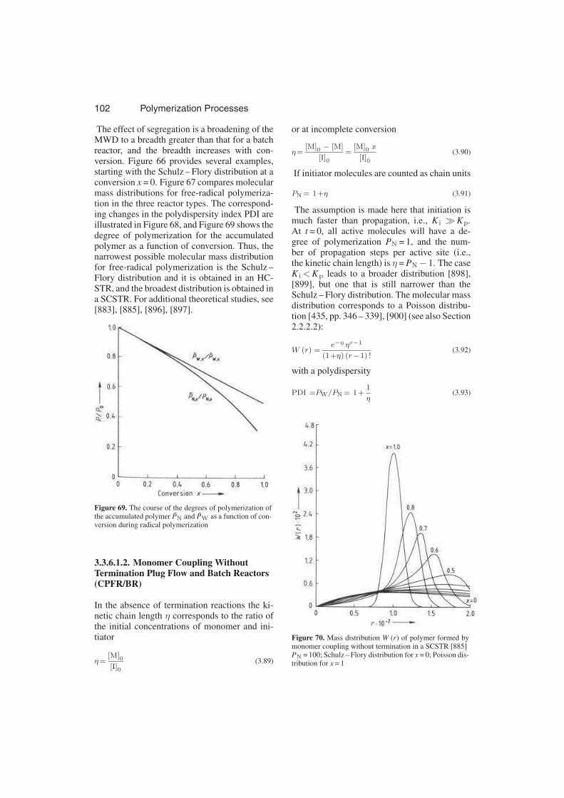
102 Polymerization Processes
The effect of segregation is a broadening of theMWD to a breadth greater than that for a batchreactor, and the breadth increases with con-version. Figure 66 provides several examples,starting with the Schulz – Flory distribution at aconversion x = 0. Figure 67 compares molecularmass distributions for free-radical polymeriza-tion in the three reactor types. The correspond-ing changes in the polydispersity index PDI areillustrated in Figure 68, and Figure 69 shows thedegree of polymerization for the accumulatedpolymer as a function of conversion. Thus, thenarrowest possible molecular mass distributionfor free-radical polymerization is the Schulz –Flory distribution and it is obtained in an HC-STR, and the broadest distribution is obtained ina SCSTR. For additional theoretical studies, see[883], [885], [896], [897].
Figure 69. The course of the degrees of polymerization ofthe accumulated polymer PN and PW as a function of con-version during radical polymerization
3.3.6.1.2. Monomer Coupling WithoutTermination Plug Flow and Batch Reactors(CPFR/BR)
In the absence of termination reactions the ki-netic chain length η corresponds to the ratio ofthe initial concentrations of monomer and ini-tiator
η=[M]0[I]0
(3.89)
or at incomplete conversion
η=[M]0 − [M]
[I]0=
[M]0 x
[I]0(3.90)
If initiator molecules are counted as chain units
PN = 1+η (3.91)
The assumption is made here that initiation ismuch faster than propagation, i.e., K i ≫Kp.
At t = 0, all active molecules will have a de-gree of polymerization PN = 1, and the num-ber of propagation steps per active site (i.e.,the kinetic chain length) is η = PN− 1. The caseK i<Kp leads to a broader distribution [898],[899], but one that is still narrower than theSchulz – Flory distribution. The molecular massdistribution corresponds to a Poisson distribu-tion [435, pp. 346 – 339], [900] (see also Section2.2.2.2):
W (r) =e−η ηr−1
(1+η) (r−1) !(3.92)
with a polydispersity
PDI =PW/PN = 1+1
η(3.93)
Figure 70. Mass distribution W (r) of polymer formed bymonomer coupling without termination in a SCSTR [885]PN = 100; Schulz – Flory distribution for x = 0; Poisson dis-tribution for x = 1
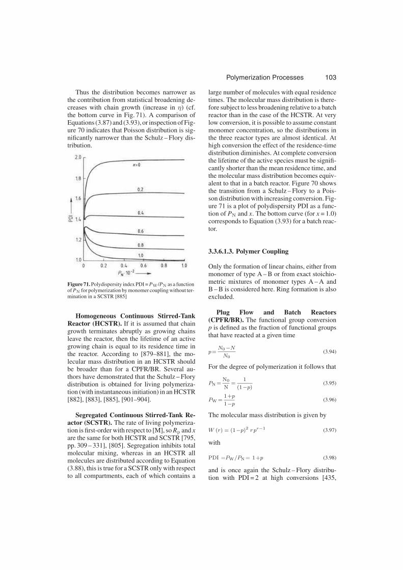
Polymerization Processes 103
Thus the distribution becomes narrower asthe contribution from statistical broadening de-creases with chain growth (increase in η) (cf.the bottom curve in Fig. 71). A comparison ofEquations (3.87) and (3.93), or inspection of Fig-ure 70 indicates that Poisson distribution is sig-nificantly narrower than the Schulz – Flory dis-tribution.
Figure 71. Polydispersity index PDI = PW/PN as a functionof PN for polymerization by monomer coupling without ter-mination in a SCSTR [885]
Homogeneous Continuous Stirred-TankReactor (HCSTR). If it is assumed that chaingrowth terminates abruptly as growing chainsleave the reactor, then the lifetime of an activegrowing chain is equal to its residence time inthe reactor. According to [879–881], the mo-lecular mass distribution in an HCSTR shouldbe broader than for a CPFR/BR. Several au-thors have demonstrated that the Schulz – Florydistribution is obtained for living polymeriza-tion (with instantaneous initiation) in an HCSTR[882], [883], [885], [901–904].
Segregated Continuous Stirred-Tank Re-actor (SCSTR). The rate of living polymeriza-tion is first-order with respect to [M], so Rp and x
are the same for both HCSTR and SCSTR [795,pp. 309 – 331], [805]. Segregation inhibits totalmolecular mixing, whereas in an HCSTR allmolecules are distributed according to Equation(3.88), this is true for a SCSTR only with respectto all compartments, each of which contains a
large number of molecules with equal residencetimes. The molecular mass distribution is there-fore subject to less broadening relative to a batchreactor than in the case of the HCSTR. At verylow conversion, it is possible to assume constantmonomer concentration, so the distributions inthe three reactor types are almost identical. Athigh conversion the effect of the residence-timedistribution diminishes. At complete conversionthe lifetime of the active species must be signifi-cantly shorter than the mean residence time, andthe molecular mass distribution becomes equiv-alent to that in a batch reactor. Figure 70 showsthe transition from a Schulz – Flory to a Pois-son distribution with increasing conversion. Fig-ure 71 is a plot of polydispersity PDI as a func-tion of PN and x. The bottom curve (for x = 1.0)corresponds to Equation (3.93) for a batch reac-tor.
3.3.6.1.3. Polymer Coupling
Only the formation of linear chains, either frommonomer of type A – B or from exact stoichio-metric mixtures of monomer types A – A andB – B is considered here. Ring formation is alsoexcluded.
Plug Flow and Batch Reactors(CPFR/BR). The functional group conversionp is defined as the fraction of functional groupsthat have reacted at a given time
p=N0−N
N0(3.94)
For the degree of polymerization it follows that
PN =N0
N=
1
(1−p)(3.95)
PW =1+p
1−p(3.96)
The molecular mass distribution is given by
W (r) = (1−p)2 rpr−1 (3.97)
with
PDI =PW/PN = 1+p (3.98)
and is once again the Schulz – Flory distribu-tion with PDI = 2 at high conversions [435,

104 Polymerization Processes
pp. 336 – 339], [873], [882], [883], [902], [905–908].
Figure 72. Molecular mass distribution W (r) of polymerformed by polymer coupling in a CPFR/BR [873]
Figure 73. Molecular mass distribution W (r) for polymer-ization by polymer coupling in three different reactors [883]
Figure 72 shows the molecular mass distri-bution at various conversions. For free-radical
polymerization the Schulz – Flory distributionalways has a PDI = 2 because ϕ, the probabil-ity of propagation, is almost always very closeto unity. This is not so for polycondensations,where p can vary from 0 to 1, and thus PDI variesfrom 1 to 2.
Figure 74. Polydispersity index PDI = PW/PN as a functionof PN for polymer coupling [885]
Homogeneous Continuous Stirred-TankReactor (HCSTR). Monomer and polymermolecules are capable of reacting with eachother throughout their entire residence time inthe reactor. Thus, according to the principle ofDenbigh [879–881], a broader molecular massdistribution is to be expected in an HCSTR thanin a batch reactor. The broad distribution of res-idence times means that material leaving the re-actor always contains a relatively large amountof monomer and polymer with a low degree ofpolymerization. On the other hand, with increas-ing molecular mass the probability of the forma-tion of very large macromolecules by the cou-pling of two smaller ones increases greatly. Cal-culations give a very broad distribution (Fig. 73)in which the number-average degree of polymer-ization PN is the same as in a batch reactor, butthe weight-average PW is much higher [883],[885], [902], [907], [909], [910]:

Polymerization Processes 105
Figure 75. Composition of the copolymer produced in a batch reactor (BR) as a function of monomer composition of thecharge as well as conversionFirst column: instantaneous composition; second column: instantaneous compositions, starting with monomer ratios[M1] : [M2] = 1 : 3, 1 : 1, and 3 : 1; third column: cumulative compositions based on the same starting ratios
PN =1
1−p
PW =1+p2
(1−p)2(3.99)
This corresponds also to a considerably higherPDI, which increases rapidly with increasingconversion (Fig. 74):
PDI =1+p2
(1−p)(3.100)
Segregated Continuous Stirred-TankReactor (SCSTR). Segregation reduces theamount of polymer with very high or very lowmolecular mass [883], [885]. Figure 73 com-pares the molecular mass distributions expectedfor the three reactor types and Figure 74 showsthe polydispersity index PDI as a function ofPN. In terms of both PN and PDI, the SCSTRlies between the CPFR/BR and the HCSTR.
Note that the conclusions drawn in the pre-ceding two sections are a result of purely the-oretical considerations, and they actually havelittle to do with practice. On the one hand, Equa-tion (3.95) (see also Fig. 62) indicates that at-taining a reasonably high degree of polymer-ization requires a very high conversion; HC-

106 Polymerization Processes
Figure 76. Ternary copolymerization in the system styrene (M1), 2,5-dichlorostyrene (M2), and acrylonitrile (M3) [912]A) Instantaneous copolymer composition (arrow point) as a function of composition of the monomer mixture (origin of thearrow); B) Partial azeotropes, where arrows outside the diagram indicate the positions of binary azeotropes
STR and SCSTR systems would therefore ap-pear inappropriate (extreme viscosities wouldbe inappropriate for a CSTR). On the otherhand, many polycondensations and polyaddi-tions are accompanied by rearrangements atthe heteroatoms, including transesterificationsor transamidations. This means that polymerwith a Schulz – Flory distribution would be ob-tained even in an HCSTR [435, pp. 336 – 339],[911].
3.3.6.1.4. Copolymerization
The theory of copolymerization kinetics is co-vered in Section 2.3. However, the performanceof the three reactor types (CPFR/BR, HCSTR,and SCSTR) were not compared and thereforethis topic is considered here.
Copolymerization in CPFR/BR Reactors.Figure 75 gives several illustrations of composi-tional drift for binary copolymerization for var-ious comonomer pairs in continuous plug flowand batch reactors. The first two columns arefor the mole fraction of monomer 1 chemicallybound in copolymer chains produced instanta-neously (over a small conversion or time in-terval) as a function of mole fraction of freemonomer 1 and of conversion. The third col-umn shows the mole fraction of monomer 1 inthe accumulated copolymer chains versus con-version. Azeotropes also occur in systems with
more than two comonomers. Figure 76 shows athree-fold combination represented in terms oftriangular coordinates. The compositions of var-ious comonomer mixtures are indicated by theorigins of arrows, with the corresponding arrowpoints showing the instantaneous compositionsof the resulting polymers. The length of an ar-row is thus a measure of the deviation betweencompositions of free monomer and copolymer.Such an arrow degenerates to a point in the caseof an azeotropic composition. A phenomenonknown as “partial azeotropy” is of interest in thecontext of multicomponent systems, with onlyone of the monomers represented by an identicalmole fraction in both copolymer and monomermixture. Thus, for ternary copolymerization
m1
m1 +m2 +m3=
[M1]
[M1] + [M2] + [M3](3.101)
A systematic computer search of the literaturehas produced copolymerization parameters for37 ternary azeotropes, 4 quaternary azeotropes,and one 5-component azeotrope [912]. Fig-ure 77 shows copolymer composition distribu-tions (CCDs) for the monomer pairs and com-positions treated in Figure 75. Copolymer ofuniform composition can be expected duringa batch polymerization only at the azeotropiccomposition, or at extremely low conversions.Strictly speaking, a copolymer is not uniform atall molecular masses even under azeotropic con-ditions. What is in fact produced is more nearly a

Polymerization Processes 107
Figure 77. Copolymer composition distributions (CCDs) for the monomer pairs of Figure 75. CCDs of completely polymer-ized batches with molar ratios [M1] : [M2] = 1 : 3 (first column), 1 : 1 (second column), and 3 : 1 (third column)The mean composition of the copolymer corresponds to that in the batch. The height of each block represents that fraction ofthe overall copolymer that has a composition within the block width of 0.05Experimental data and calculated values as a function of f 1; 60 ◦C, [I] = 1 g/L azobisisobutyronitrile
statistical distribution about a mean [913], [914],although at high degrees of polymerization thisvariation is minor in comparison to the hetero-geneity that results from progressive changes inthe composition of the monomer mixture withconversion.
Copolymerization in an HCSTR. In anHCSTR operating at steady state the tempera-ture and concentration are constant in both spaceand time. The result is therefore a chemicallyuniform copolymer. In the limiting case of verylow conversion, the copolymer composition cor-responds to the predictions of Equation (2.121)and Figure 75 when concentrations of monomerin the inlet stream are used to calculate monomer
composition. The only other situation in whichthe composition of the copolymer correspondsprecisely to the composition of the monomermixture in the feed is the technically unrealis-tic limit of complete conversion, which wouldrequire impractically long residence times. Theinstantaneous copolymer equation, of course,can always be used when monomer composi-tion in the exit stream is used (as opposed toinlet stream) [915], [916]. Figure 78 shows thechange in steady-state copolymer compositionfor the system styrene/acrylonitrile (40/60) asa function of conversion. Thus, a copolymerwith a particular composition can be made inpractice (at least approximately) either by estab-lishing in advance a preferred composition for

108 Polymerization Processes
the monomer feed and then varying the extent ofconversion, or by varying the feed compositionat a fixed conversion.
Figure 78. Continuous copolymerization in the systemstyrene ( f 1 = 0.4) / acrylonitrile ( f 2 = 0.6) [915]Composition of accumulated copolymer Fi as a function ofconversion
Copolymerization in a SCSTR. It wasnoted earlier that true mixing is often less com-plete than envisioned by the HCSTR concept ina polymerization reactor operating under condi-tions of high viscosity. Most industrial reactorsprobably provide an efficiency of mixing thatfalls between the values assumed for the HCSTRand SCSTR. By introducing certain simplify-ing assumptions, O’Driscoll and Knorr [917]were able to calculate CCDs corresponding tothe three reactor models CPFR/BR, HCSTR, andSCSTR. Figure 79 A shows a representation ofa typical instantaneous copolymer compositiondiagram. Figure 61 B shows CCD curves for thethree ideal reactor types at two conversions. Thefeed composition is fixed at f 1 = 0.4 for all casesshown. Open circles represent mean copolymercompositions F1 which are not very different inthe three cases. The differences in the CCDs aregreater, however. At 35 % conversion the CCDis relatively narrow in a CPFR/BR (curve 1),absolutely uniform in an HCSTR (curve 2), andalready quite nonuniform in a SCSTR (curve3). In the latter, more than 10 % of the poly-mer is homopolymer of monomer 2. A SCSTRalways provides several batch-reactor-like com-partments with very long residence times, highconversions, and extreme changes in monomerand copolymer compositions. At 73 % conver-sion the CCD shows nearly as much nonuni-formity with a CPFR/Batch (curve 4) as with aSCSTR (curve 6), only the HCSTR (curve 5)
again producing a uniform CCD. The amountof homopolymer produced is, of course, greaterat 73 % than at 35 % conversion.
Figure 79. Copolymerization of methyl methacrylate(M1) – vinyl acetate (M2) in three types of reactor: BR,HCSTR, and SCSTR [917]A) Instantaneous composition, calculated with r1 = 20,r2 = 0.015; B) Copolymer composition distribution (CCD)at f 1 = 0.4, 35 and 73 % conversion in a BR (curves 1 and4), a HCSTR (2 and 5), and a SCSTR (3 and 6)
Curve: 1 2 3 4 5 6
Conversion x: 0.35 0.35 0.35 0.73 0.73 0.73
3.3.6.1.5. Long-Chain Branching andCross-Linking
The amounts of long-chain branching and cross-linking (with gel formation) obtained in free-radical polymerizations depend strongly on theresidence-time distribution of the reactor and theconversion (or polymer concentration). Com-pared to the HCSTR, the CPFR/BR givesless long-chain branching, cross-linking (cross-linking density), and gel for the same con-version. Apparenty, calculations on long-chainbranching and cross-linking in a SCSTR havenot been performed; however, one could specu-late that the extent of long-chain branching in aSCSTR would lie between that for a CPFR/BRand HCSTR. Graessley et al. [918] have car-ried out theoretical modeling and experimentsfor CPFR/BR and HCSTR using vinyl acetatehomopolymerization. Their experimental poly-dispersity data are shown in Figure 80 forCPFR/BR and HCSTR. Note that long-chainbranching is due to chain transfer to polymer andaddition of polymeric radicals to terminal doublebonds on polymer chains and that such branch-ing leads to increases in the polydispersity in-dex starting at 2.0 for linear chains produced at
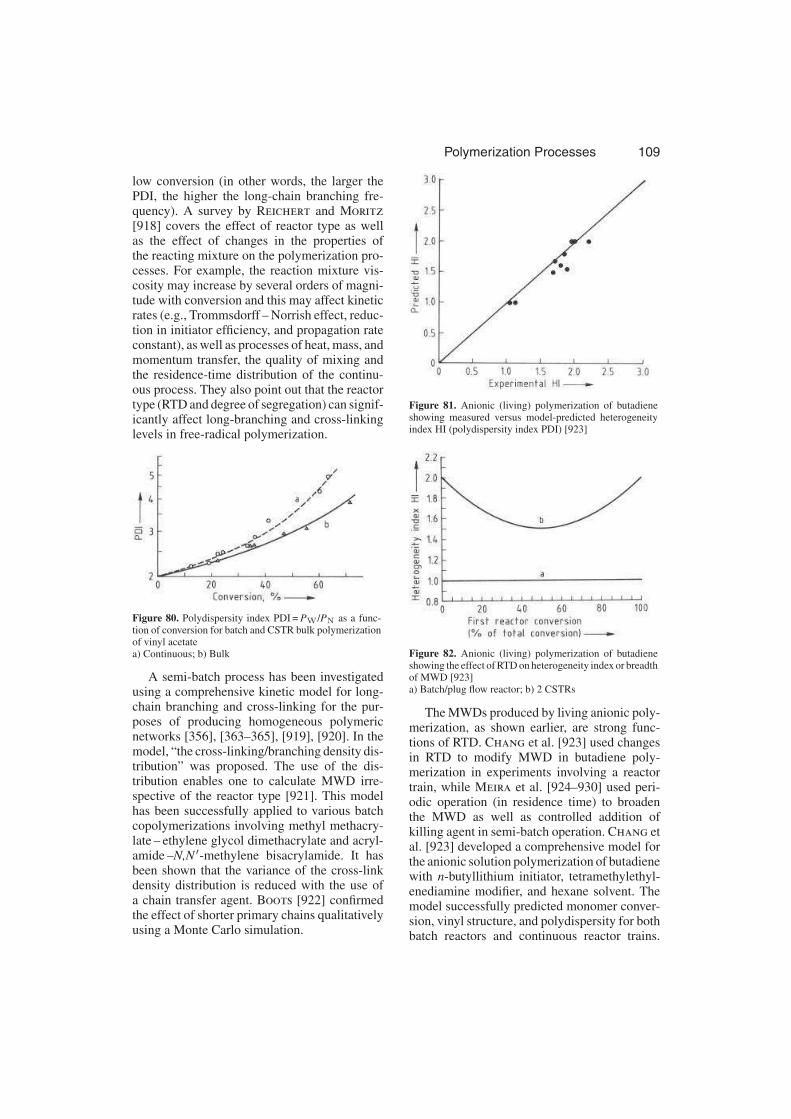
Polymerization Processes 109
low conversion (in other words, the larger thePDI, the higher the long-chain branching fre-quency). A survey by Reichert and Moritz
[918] covers the effect of reactor type as wellas the effect of changes in the properties ofthe reacting mixture on the polymerization pro-cesses. For example, the reaction mixture vis-cosity may increase by several orders of magni-tude with conversion and this may affect kineticrates (e.g., Trommsdorff – Norrish effect, reduc-tion in initiator efficiency, and propagation rateconstant), as well as processes of heat, mass, andmomentum transfer, the quality of mixing andthe residence-time distribution of the continu-ous process. They also point out that the reactortype (RTD and degree of segregation) can signif-icantly affect long-branching and cross-linkinglevels in free-radical polymerization.
Figure 80. Polydispersity index PDI = PW/PN as a func-tion of conversion for batch and CSTR bulk polymerizationof vinyl acetatea) Continuous; b) Bulk
A semi-batch process has been investigatedusing a comprehensive kinetic model for long-chain branching and cross-linking for the pur-poses of producing homogeneous polymericnetworks [356], [363–365], [919], [920]. In themodel, “the cross-linking/branching density dis-tribution” was proposed. The use of the dis-tribution enables one to calculate MWD irre-spective of the reactor type [921]. This modelhas been successfully applied to various batchcopolymerizations involving methyl methacry-late – ethylene glycol dimethacrylate and acryl-amide –N,N ′-methylene bisacrylamide. It hasbeen shown that the variance of the cross-linkdensity distribution is reduced with the use ofa chain transfer agent. Boots [922] confirmedthe effect of shorter primary chains qualitativelyusing a Monte Carlo simulation.
Figure 81. Anionic (living) polymerization of butadieneshowing measured versus model-predicted heterogeneityindex HI (polydispersity index PDI) [923]
Figure 82. Anionic (living) polymerization of butadieneshowing the effect of RTD on heterogeneity index or breadthof MWD [923]a) Batch/plug flow reactor; b) 2 CSTRs
The MWDs produced by living anionic poly-merization, as shown earlier, are strong func-tions of RTD. Chang et al. [923] used changesin RTD to modify MWD in butadiene poly-merization in experiments involving a reactortrain, while Meira et al. [924–930] used peri-odic operation (in residence time) to broadenthe MWD as well as controlled addition ofkilling agent in semi-batch operation. Chang etal. [923] developed a comprehensive model forthe anionic solution polymerization of butadienewith n-butyllithium initiator, tetramethylethyl-enediamine modifier, and hexane solvent. Themodel successfully predicted monomer conver-sion, vinyl structure, and polydispersity for bothbatch reactors and continuous reactor trains.
110 Polymerization Processes
Figure 81 shows predicted versus measuredheterogeneity index (polydispersity index orMW/MN), covering the range from that obtainedin a PFR or batch reactor to that obtained in asingle CSTR. Figure 82 shows the polydisper-sity for 2 CSTRs of equal volume in series withequal conversion of monomer in each, giving thelowest value of polydispersity, 1.5.
3.3.6.2. Reactor Dynamics and Stability
Reichert and Moritz [918] discuss reactor sta-bility and safety under the subtopics thermal andconcentration stability. The strong nonlinear de-pendence of polymerization rate (or heat pro-duction rate) on temperature is due to the Ar-rhenius dependence of rate on temperature andto the large activation energy and heat of poly-merization. The dynamic behavior of polymerreactors is therefore greatly affected by temper-ature. The influence of the nonlinear dependenceof polymerization rate on monomer concentra-tion, on reactor dynamics is much smaller thanthat for thermal effects. Both static and dynamicinstabilities may occur when stability limits arecrossed. The reactor is statically unstable if tem-perature and conversion rapidly move from onestate to another as if alternately experiencing “ig-nition” and “extinction”. Dynamic instabilitiesgive rise to periodic changes in temperature andmonomer conversion with certain phase shiftsobserved [931], [932]. Thermal instabilities mayoccur in various reactor types (CSTR, PFR, non-ideal reactors) [933], [934]. Henderson [935]points out that for all prior publications on mul-tiple steady states and instability for free radicalpolymerization in a CSTR, three basic assump-tions were made:
1) The heat-transfer coefficient of the vesselwall does not change with monomer conver-sion
2) The viscous dissipation term for the agitationis negligible
3) Perfect mixing (ideal RTD and micromixing)
Mechanical work of the agitator can be a sig-nificant factor in the energy balance for a pilot-scale reactor (perhaps for solution and bulk poly-merization, but not for suspension and emulsionpolymerization), while it is almost negligible forcommercial scale. Assumptions (2) and (3) may
be valid for low-viscosity solution processes;however, in bulk polymerization, the viscositycan increase by several orders of magnitude and,therefore, all 3 assumptions are questionable.Henderson again points out that a thermal run-away can occur when:
1) The process side heat-transfer coefficient de-creases significantly
2) The agitator provides insufficient mixing ofthe reaction mass, allowing hot spots to de-velop
3) The agitator is putting more mechanicalwork into the system than designed for
Ray et al. [788–791], [936–945] have madethe most significant contributions to the under-standing of polymer reactor dynamics and sta-bility. Comprehensive reactor models were de-veloped for a range of polymerization processesand reactor types: nonisothermal solution homo-and copolymerization in a CSTR [931], [939],[940]; batch and continuous emulsion polymer-ization reactors [788–791], [941], [942]; hetero-geneous coordination polymerization for bothliquid and gas dispersion reactors [943–945].The contributions by Ray et al. are notable notonly for the comprehensive mathematical mod-els but also for attempts at experimental verifi-cation. In this regard, the experimental investi-gation of the effect of chain-transfer agents onthe stability of continuous latex reactors is veryrevealing. Whereas under most operation con-ditions the continuous emulsion polymerizationof styrene is stable, the addition of a chain-trans-fer agent to the recipe can lead to sustained os-cillations. Some of Ray’s general conclusionsinclude:
1) Bifurcation analysis reveals a parame-ter space rich in dynamic phenomena. Itconfirms limit cycle behavior (in whichmonomer conversion does not smoothly ap-proach a constant steady-state value, butrather oscillates with constant frequency andamplitude indefinitely) and analyzes the sta-bility of periodic branches in detail providinguseful guidelines for experimental design.
2) Full-scale reactors exhibit dynamic behaviorof high complexity.
3) Semi-batch reactors can be operated underconditions that insure a fast approach to a
Polymerization Processes 111
steady-state operating value, hence permit-ting almost perfect control. The possibility ofoscillatory behavior was, however, demon-strated.
4) Multiplicity (multiple steady states) oc-curs under isothermal conditions due to theTrommsdorff – Norrish effect and there ap-pears to be no relationship between phenom-ena causing multiplicity and reactor oscilla-tions.
5) The PSD plays a major role in latex reac-tor stability. Models which calculate only amean diameter d (and not the full PSD) can-not predict oscillations under any operatingconditions.
6) Polymer particle multiplicity, which leads topolymer melting and sticking (in gas-phaseheterogeneous coordination polymerization,such as UNIPOL) can cause a thermal run-away of the reactor (UNIPOL is open-loopunstable). Multiplicity and Hopf bifurcationof the fluidized-bed reactor can lead to run-away and long periods of slowly damped os-cillations. The reactor is prone to runawayeven under feedback control because of cool-ing limitations and nonlinear sensitivity toprocess disturbances.
Lu and Brooks [946] have confirmed that la-tex reactor startup policy can have a significanteffect on reactor stability.
It is clear, based on these studies of reactorstability, that a comprehensive dynamic modelof the polymerization reactor is required to prop-erly design a continuous manufacturing process(process stability, control, and startup proce-dures should be considered at the design stage).The interactions are too complex to permit an ef-fective design based on costly experimentationalone.
3.3.6.3. On-Line Monitoring and Control
The goals in commercial polymerizations areconsistent polymer properties, high productiv-ity, and safe operation achieved in the most eco-nomic manner possible. Polymerizations (par-ticularly ionic and free-radical) are very sensi-tive to temperature and impurities (radical scav-engers and poisons at ppm levels) and, therefore,adjustments may have to be made during poly-merization. Process models when applied in real
time require measurements and parameter up-dating to track and control the process. The needfor monitoring the polymerization is clear andto be most effective in controlling the process,on-line monitoring is highly desirable. A surveyof on-line sensors for polymerization reactorswas made by Chien and Penlidis [947]. Al-though considerable advances have been madein polymer reaction engineering over the pasttwo decades, sensor technology for on-line mon-itoring is still in its infancy. The major problemhas been the on-line measurement of polymerand particle properties (copolymer composition,molecular mass averages, long-chain branching,as well as cross-linked gel content and poly-mer particle size distribution in suspension andemulsion polymerization). Sensors in the reac-tion mixture are readily fouled by sticky polymerand polymer particles. Another factor to explainthe lack of progress is the fact that sensor devel-opment is a multidisciplinary task with exper-tise required in statistics, mathematical model-ing, process understanding, reactor design, ad-vanced control concepts, electronics, and in-strumentation engineering [947]. Even the mea-surement of polymer properties off-line is diffi-cult (e.g., measurement of molecular mass aver-ages and long-chain-branching frequencies forheterogeneous copolymers [870]). Chien andPenlidis [947] classify sensors as those whichmonitor reactor operation [by measuring tem-perature, pressure, flows and level (of reactionmixture in the reactor)], and those that moni-tor polymer properties (e.g., by measuring den-sity, viscosity, concentrations, copolymer com-position, particle size, using densitometers, vis-cometers, gas and liquid chromatographs, IR andUV spectrophotometers, light scattering, ultra-sonics, fiber-optic techniques, robotics, reactorenergy balances, and state estimation/filteringtechniques). Most of the commercial applica-tions of on-line monitoring involve those whichmonitor reactor operation, although reactor en-ergy balances are commonly used to monitormonomer conversion. The main problem withthe successful use of reactor energy balances liesin the evaluation of the transient accumulationterms (time derivatives of temperature) and inaccounting for the propagation of measurementerrors (temperature and flow rate) into the cal-culated heat release term. Acceptable results are

112 Polymerization Processes
often obtained through rapid sampling and thenaveraging or filtering all the measurements atregular short intervals [949].
Two promising on-line monitoring tech-niques are based on the use of ultrasound andNIRS (near infrared spectroscopy) [948]. Ul-trasonic velocity and attenuation measurementshave been used for monitoring high-temperaturecomposition in extruders and melt-transfer lines;high-temperature imaging studies in extruders;and for ultrasonic spectroscopy of dispersions.NIRS is an older technique which has been im-proved by newly available computing power.It is the most promising process spectroscopyavailable at present because of its process com-patability and ability to analyze multicomponentmixtures. NIRS has been applied as an on-linemonitoring technique for both extruders used forchemical modification and polymer reactors.
The on-line monitoring and control of poly-mer and polymer particle properties should pro-vide a major improvement in product consis-tency and productivity.
There have been a number of excellent re-views on control of polymerization reactors[947], [949], [950]. Most industrial control prac-tice to date has centered around batch reactorsequencing and the control of process variablessuch as temperature, pressure, and viscosity. Re-actor energy balances, as mentioned earlier, havealso been used to infer polymer production ratesand monomer conversion.
Much of the academic literature has focusedon the computation of optimal operating poli-cies for batch reactors by using nonlinear pro-gramming or the maximum principle [374].These policies are open-loop in that they provideoptimal feed and temperature policies versustime. Kozub and MacGregor [951] presenteda much simpler solution to the optimal trajec-tory problems based on an “instantaneous prop-erty” approach. This latter approach is applica-ble only to chain-growth polymerizations (seeSection 2.2 for details of instantaneous propertycalculations), but it allows for the feedback im-plementation of these optimal policies via non-linear control.
Due to the lack of sufficient on-line sen-sors to monitor polymer properties of interest orbecause some property measurements are onlyavailable infrequently from quality control lab-oratories, various methods for inferring or es-
timating these properties on-line by using fun-damental mathematical models have been pro-posed. State estimators such as the Kalman Filter[952], [953] and recursive parameter estimators[954] have been advocated to update model pa-rameters and predict polymer properties.
Feedback control over measured or inferredproperties in continuous reactors has been ac-complished by using empirical models [955],[956].
However, in spite of the many advances thathave been made in the methodology for the ad-vanced control of polymerization reactors, thereare still few industrial applications.
Figure 83. Continuous emulsion polymerization in a reac-tor train with a split feed (small polymer particle nucleatingreactor followed by one or more larger finishing reactors)[956]a) Small seeding reactor; b) First large reactor in train
To again emphasize the point that controlproblems should be considered at the designstage of a polymer manufacturing process, ref-erence is made to the well-known stability prob-lems that are experienced with continuous emul-sion polymerization (in a single CSTR) involv-ing monomer(s) that experience Case I kinetics(e.g., vinyl acetate and vinyl chloride). Moderncontrol theory did not provide suitable controlmethodology for the single CSTR. It was de-cided, therefore to go back to the design stage,redesign the process by using a dynamic reac-tor model and minimize control problems at thedesign stage. The new design which is shownin Figure 83 has almost trivial control problems[949], [956]. Experimental verification of the in-crease in stability of this new design may be seenin Figure 84. The initial response (conversion

Polymerization Processes 113
Figure 84. Conversion responses to CSTR reactor system shown in Figure 83 for continuous emulsion polymerization of vinylacetatePart A: operation with a single CSTR (shows sustained oscillations)Part B: switching over to seed reactor followed by one finishing reactor (responses for both reactors are shown, with verystable response for downstream reactor and minor disturbance for seed reactor) [611]
versus time) is for a single CSTR. The follow-ing two responses are for the small seed reactorand for the larger finishing reactor.
4. References
1. J. V. Seppala, K. H. Reichert: “Trends in
Polymer Reaction Engineering,” Kem.-Kemi
17 (1990) 346.
2. W. H. Ray: “Current Problems in
Polymerization Reaction Engineering,” ACS
Symp. Ser. 226 (1983) 101.
3. Ullmann, 4th ed., 19, 109.
4. H. Gerrens, Chem. Ing. Tech. 52 (1980) 477;
Chemical Engineering 4 (1981) 1.
5. H. Gerrens, Chem. Tech. (1982) June, 380;
(1982) July, 434.
6. D. H. Sebastian, J. A. Biesenberger:
Polymerization Engineering, Wiley, New York
1983.
7. K. H. Reichert, H. U. Moritz: “Polymer
Reaction Engineering,” Comprehensive
Polymer Science, vol. 3, Pergamon Press, New
York 1989, p. 327.
General References
8. P. J. Flory: Principles of Polymer Chemistry,
Cornell University Press, Ithaca, New York
1953.
9. R. W. Lenz: Organic Chemistry of Synthetic
High Polymers, Wiley-Interscience, New York
1968.
10. F. W. Billmeyer: Te xbook of Polymer Science,
Wiley-Interscience, New York 1971.
11. D. H. Solomon (ed.): Step-Growth
Polymerization, Marcel Dekker, New York
1972.
12. F. A. Bovey, F. W. Winslow (eds.):
Macromolecules, Academic Press, New York
1979.
13. G. Odian: Principles of Polymerization,
Wiley-Interscience, New York 1981.
14. A. Rudin: The Elements of Polymer Science
and Engineering, Academic Press, Orlando,
Fla. 1982.
15. P. C. Hiemenz: Polymer Chemistry, Marcel
Dekker, New York 1984.
16. S. K. Gupta, A. Kumar: Reaction Engineering
of Step Growth Polymerization, Plenum Press,
New York 1987.
17. R. B. Seymour, C. E. Carraher: Polymer
Chemistry, Marcel Dekker, New York 1988.
Specific References
18. J. L. Stanford, R. F. T. Stepto, J. Chem. Soc.,
Faraday Trans. 71 (1975) 1292.
19. R. F. T. Stepto: “Intra-Molecular Reaction and
Gelation in Condensation or Random
Polymerization,” in R. N. Haward (ed.):

114 Polymerization Processes
Developments in Polymerization-3, Applied
Science Publ., Barking 1982, p. 81.
20. W. H. Carothers, Trans. Faraday Soc. 32
(1936) 39.
21. P. J. Flory: Principles of Polymer Chemistry,
Cornell University Press, Ithaca, N.Y. 1953,
chap. 8.
22. W. Burchard, Polymer 20 (1979) 589.
23. D. Durand, C. M. Bruneau, Makromol. Chem.
180 (1979) 2947.
24. T. M. Orlova, S.-S. A. Pavlova, L. V.
Dubrovina, J. Polym. Sci., Polym. Chem. Ed.
17 (1979) 2209.
25. F. Lopez-Serrano, J. M. Castro, C. W.
Macosko, M. Tirrell, Polymer 21 (1980) 263.
26. E. Ozizmir, G. Odian, J. Polym. Sci., Polym.
Chem. Ed. 18 (1980) 2281.
27. W. H. Abraham, Ind. Eng. Chem. Fundam. 2
(1963) 221.
28. H. Kilkson, Ind. Eng. Chem. Fundam. 3
(1964) 281.
29. J. A. Biesenberger, AIChE J. 11 (1965) 369.
30. H. Kilkson, Ind. Eng. Chem. Fundam. 7
(1968) 354.
31. T. T. Szabo, J. F. Leathrum, J. Appl. Polym. Sci.
13 (1969) 477.
32. W. H. Ray, J. Macromol. Sci. Rev. Macromol.
Chem. C 8 (1972) 1.
33. W. H. Ray: “Polymerization Reaction
Engineering,” in L. Lapidus, N. R. Amundson
(eds.): Chemical Reactor Theory,
Prentice-Hall, Englewood Cliffs, N. J. 1977,
p. 532.
34. N. A. Dotson, Macromolecules 22 (1989)
3690.
35. P. W. Morgan: Condensation Polymers by
Interfacial and Solution Methods,
Wiley-Interscience, New York 1965.
36. F. Millich, C. E. Carraher, Jr., J. Preston (eds.):
Interfacial Synthesis, vol. III, Marcel Dekker,
New York 1982.
37. P. J. Flory, J. Am. Chem. Soc. 63 (1941) 3083.
38. P. J. Flory, J. Am. Chem. Soc. 63 (1941) 3091.
39. P. J. Flory, J. Am. Chem. Soc. 63 (1941) 3096.
40. C. Cozewith, W. W. Graessley, G. Ver Strate,
Chem. Eng. Sci. 34 (1979) 245.
41. S. K: Gupta, A. Kumar: Reaction Engineering
of Step Growth Polymerization, Plenum Press,
New York 1987, chap. 4.
42. W. H. Stockmayer, J. Chem. Phys. 11 (1943)
45.
43. W. H. Stockmayer, J. Chem. Phys. 12 (1944)
125.
44. W. H. Stockmayer, J. Polym. Sci. 9 (1952) 69;
J. Polym. Sci. 11 (1953) 11.
45. M. Gordon, Proc. R. Soc. London A 268
(1962) 240.
46. M. Gordon, S. B. Ross-Murphy, Pure Appl.
Chem. 43 (1975) 1.
47. M. Gordon, W. B. Temple: “The Graph-Like
State of Matter and Polymer Science,” in A. T.
Balaban (ed.): Chemical Application of Graph
Theory, Academic Press, New York 1976,
p. 299.
48. S. I. Kuchanov, S. V. Koralev, S. V. Panyukov,
Adv. Chem. Phys. 72 (1988) 115.
49. D. S. Pearson, W. W. Graessley,
Macromolecules 11 (1978) 528. O. Durand,
C. M. Bruneau, Makromol. Chem. 83 (1982)
1007, 1021.
50. D. R. Miller, C. W. Macosko, J. Polym. Sci.
Polym. Phys. Ed. 26 (1988) 1.
51. C. W. Macosko, D. R. Miller, Macromolecules
9 (1976) 199.
52. D. R. Miller, C. W. Macosko, Macromolecules
9 (1976) 206.
53. D. R. Miller, C. W. Macosko, Macromolecules
11 (1978) 656.
54. D. Durand, C. M. Bruneau, Polymer 24 (1983)
587.
55. M. Gordon, G. R. Scantlebury, Proc. R. Soc.,
London, A 292 (1966) 380. M. Gordon, G. N.
Malcom, Proc. Roy. Soc, London, Ser. A 292
(1966) 29. D. Durand, C. M. Bruneau, Polymer
24 (1983) 592.
56. D. R. Miller, C. W. Macosko, Macromolecules
13 (1980) 1063.
57. R. W. Kilb, J. Phys. Chem. 62 (1958) 969.
58. M. Gordon, G. R. Scantlebury, J. Polym. Sci.,
Part C 16 (1968) 3933.
59. W. B. Temple, Makromol. Chem. 160 (1972)
277.
60. H. Galina, A. Szustalewicz, Macromolecules
22 (1989) 3124.
61. H. Tobita, Ph. D. Thesis, McMaster University,
Hamilton, Canada 1990.
62. A. N. Dotson, R. Galvan, C. W. Macosko,
Macromolecules 21 (1988) 2560.
63. O. Saito, J. Phys. Soc. Jpn. 13 (1958) 198.
64. O. Saito: “Statistical Theory of Crosslinking”,
in M. Dole (ed.): The Radiation of
Macromolecules, Academic Press, New York
1972, p. 223.
65. S. I. Kuchanov, L. M. Pis’men, Polym. Sci.
USSR (Engl. Transl.) 14 (1972) 985. M.
Gordon, G. N. Malcom, Proc. R. Soc. London
A, 292 (1966) 29. D. Durand, C. M. Bruneau,
Polymer 24 (1983) 592.
66. K. Dusek, Makromol. Chem. Suppl. 2 (1979)
35.

Polymerization Processes 115
67. E. Donoghue, J. H. Gibbs, J. Chem. Phys. 70
(1979) 2346.
68. S. I. Kuchanov, Ye. S. Povolotskaya, Polym.
Sci. USSR (Engl. Transl.) 24 (1982) 2499.
69. S. I. Kuchanov, Ye. S. Povolotskaya, Polym.
Sci. USSR (Engl. Transl.) 24 (1982) 2512.
70. J. Mikes, K. Dusek, Macromolecules 15
(1982) 93.
71. S. R. Broadbent, J. M. Hammersley, Proc.
Cambridge Philos. Soc. 53 (1957) 629.
72. J. M. Hammersley, Proc. Cambridge Philos.
Soc. 53 (1957) 642.
73. H. L. Frisch, J. M. Hammersley, J. Soc. Ind.
Appl. Math. 11 (1963) 894.
74. J. W. Essam: “Percolation and Cluster Size,” in
C. Domb, M. Green (eds.): Phase Transitions
and Critical Phenomena, Academic Press,
New York 1972, p. 197.
75. S. Kirkpatrick, Rev. Mod. Phys. 45 (1973) 574.
76. C. Domb, E. Stoll, T. Schneider, Contemp.
Phys. 21 (1980) 577.
77. D. Stauffer: Introduction to Percolation
Theory, Taylor and Francis, London 1985.
78. D. Stauffer, A. Conoglio, M. Adam, Adv.
Polym. Sci. 44 (1982) 103.
79. D. Durand: “Network Formation – From Basic
Theories Towards More Realistic Models,” in
R. A. Pethrick (ed.): Polymer Yearbook 3,
Harwood Academic Publishers, New York
1986, p. 229.
80. P. G. de Gennes: Scaling Concepts in Polymer
Physics, Cornell University Press, Ithaca, N.Y.
1979, p. 139.
81. O. Vogl: “Kinetics of Aldehyde
Polymerization,” C. H. Bamford, C. F. H.
Tipper (eds.): Comprehensive Chemical
Kinetics, vol. 15, Elsevier, Amsterdam 1976,
chap. 5.
82. O. Vogl: “Aldehyde Polymers,” in
Encyclopedia of Polymer Science and
Engineering, vol. 1, Wiley-Interscience, New
York 1985, p. 623.
83. R. N. Noyes: “Cage Effect,” in Encyclopedia
of Polymer Science and Technology, vol. 2,
Wiley-Interscience, New York 1965, p. 796.
84. G. Odian: Principles of Polymerization,
Wiley-Interscience, New York 1981, p. 216.
85. H. Kiefer, T. G. Traylor, J. Am. Chem. Soc. 89
(1967) 6667.
86. E. Niki, Y. Kamiya, J. Am. Chem. Soc. 96
(1974) 2129.
87. G. T. Russell, D. H. Napper, R. G. Gilbert,
Macromolecules 21 (1988) 2141.
88. S. Zhu, A. E. Hamielec, Macromolecules 22
(1989) 3098.
89. S. S. Ivanchev, Polym. Sci. USSR, (Engl.
Transl.) 20 (1978) 2157.
90. V. R. Kamath, Mod. Plast. 58 (1981) Sept.,
106.
91. K. Y. Choi, W. R. Liang, G. D. Lei, J. Appl.
Polym. Sci. 35 (1988) 1547.
92. M. A. Villalobos, M. Eng. Thesis, McMaster
University, Hamilton, Canada 1989.
93. F. R. Mayo, J. Am. Chem. Soc. 90 (1968) 1289.
94. W. D. Graham, J. G. Green, W. A. Pryor, J.
Org. Chem. 44 (1979) 907.
95. F. R. Mayo, J. Am. Chem. Soc. 75 (1953) 6133.
96. A. W. Hui, A. E. Hamielec, J. Appl. Polym. Sci.
16 (1972) 749.
97. A. Husain, A. E. Hamielec, J. Appl. Polym.
Sci. 22 (1978) 1207.
98. N. J. Barr, W. I. Bengough, G. Beveridge, G. B.
Park, Eur. Polym. J. 14 (1978) 245.
99. H. F. Kaufmann, Makromol. Chem. 180
(1979) 2649, 2665, 2681.
100. Y. K. Chong, E. Rizzardo, D. H. Solomon, J.
Am. Chem. Soc. 105 (1983) 7761.
101. C. W. Wilson III, E. R. Santee, Jr., J. Polym.
Sci., Part C 8 (1965) 97.
102. G. Talamini, G. Vidotto, Makromol. Chem.
100 (1967) 48.
103. T. G. Fox, H. W. Schnecko, Polymer 3 (1962)
575.
104. T. Otsu, B. Yamada, M. Imoto, J. Macoromol.
Sci. Chem. 1 (1966) 61.
105. F. S. Dainton, K. J. Ivin, Nature 162 (1948)
705.
106. H. Sawada: Thermodynamics of
Polymerization, Marcel Dekker, New York
1976.
107. H. W. McCormick, J. Polym. Sci. 25 (1957)
488.
108. T. P. Davis, K. F. O’Driscoll, M. C. Piton, M. A.
Winnik, Macromolecules 22 (1989) 2785.
109. M. J. Ballard et al., Macromolecules 19 (1986)
1303.
110. P. J. Flory: Principles of Polymer Chemistry,
Cornell University Press, Ithaca, N.Y. 1953,
p. 127.
111. K. Horie, I. Mita, H. Kambe, J. Polym. Sci.
Polym. Chem. Ed. 6 (1968) 2663.
112. M. Stickler, Makromol. Chem. 184 (1983)
2563.
113. K. Ito, Polym. J. (Tokyo) 16 (1984) 761.
114. G. C. Eastmond: “The Kinetics of
Free-Radical Polymerization of Vinyl
Monomers in Homogeneous Solution,” in
C. H. Bamford, C. F. H. Tipper (eds.):
Comprehensive Chemical Kinetics, vol. 14 A,
Elsevier, Amsterdam 1976, chap. 1.
116 Polymerization Processes
115. J. C. Bevington, H. W. Mellville, R. P. Taylor,
J. Polym. Sci. 12 (1954) 449.
116. G. V. Schulz, G. Henrici-Olive, S. Olive,
Makromol. Chem. 31 (1959) 88.
117. C. H. Bamford, G. C. Eastmond, D. Whittle,
Polymer 10 (1969) 771.
118. M. Stickler, D. Panke, A. E. Hamielec, J.
Polym. Sci., Polym. Chem. Ed. 22 (1984) 2243.
119. G. V. Schulz, G. Haborth, Makromol. Chem. 1
(1948) 106.
120. A. M. North: “The Influence of Chain
Structure on the Free-Radical Termination
Reaction,” in A. D. Jenkins, A. Ledwith (eds.):
Reactivity, Mechanism and Structure in
Polymer Chemistry, Wiley-Interscience, New
York 1974, chap. 5.
121. K. F. O’Driscoll: “Kinetics of Bimolecular
Termination,” in Comprehensive Polymer
Science, vol. 3 Pergamon Press, London 1989,
p. 161.
122. I. Mita, K. Horie, J. Macromol. Sci., Rev.
Macromol. Chem. Phys. C 27 (1987) 91.
123. A. W. Hui, A. E. Hamielec, J. Polym. Sci., Part
C 25 (1968) 167.
124. J. H. Duerksen, A. E. Hamielec, J. Polym. Sci.
25 (1968) 155.
125. G. Z. A. Wu, L. A. Denton, R. L. Laurence,
Polym. Eng. Sci. 22 (1982) 1.
126. C. J. Kim, A. E. Hamielec, Polymer 25 (1984)
845.
127. G. C. Eastmond: “Chain Transfer, Inhibition
and Retardation,” in C. H. Bamford, C. F. H.
Tipper (eds.): Comprehensive Chemical
Kinetics, vol. 14 A, Elsevier, Amsterdam 1976,
chap. 2.
128. C. H. Bamford, W. G. Barb, A. D. Jenkins, P. F.
Onyon: The Kinetics of Vinyl Polymerization
by Free Radical Mechanism, Butterworth
Publications, London 1958.
129. C. H. Bamford: “Radical Polymerization,” in
Encyclopedia of Polymer Science and
Technology, vol. 13, Wiley-Interscience, New
York 1988, p. 708.
130. J. Brandrup, E. H. Immergut (eds.): Polymer
Handbook, Wiley-Interscience, New York
1975.
131. Z. Tadmor, J. A. Biesenberger, Ind. Eng.
Chem. Fundam. 5 (1966) 336. A. E.
Hamielec, J. W. Hodgins, K. Tebbens, AIChE
J. 13 (1967) 1087.
132. R. Cintron-Cordero, R. A. Mostello, J. A.
Biesenberger, Canad. J. Chem. Eng. 46
(1968) 434.
133. L. H. Peebles, Jr.: “Rates of Polymerization,
Average Molecular Weights, and Molecular
Weight Distribution of Polymers,” in J.
Brandrup, E. H. Immergut (eds.): Polymer
Handbook, vol. II, Wiley-Interscience, New
York 1975, p. 405.
134. H. Tompa: “The Calculation of Mole-Weight
Distributions from Kinetic Schemes,” in C. H.
Bamford, C. F. H. Tipper (eds.):
Comprehensive Chemical Kinetics, Elsevier,
Amsterdam 1976, chap. 7.
135. M. Tirrell, R. Galvan, R. L. Laurence:
“Polymerization Reactors,” in J. J. Carberry,
A. Varma (eds.): Chemical Reaction and
Reactor Engineering, Marcel Dekker, New
York 1987, chap. 11.
136. D. J. P. Harrison, W. R. Yates, J. F. Johnson, J.
Macromol. Sci. Rev. Macromol. Chem. C 25
(1985) 481.
137. M. Andreis, J. L. Koenig, Adv. Polym. Sci. 89
(1989) 69.
138. S. Shiga, Polym. Plast. Technol. Eng. 282
(1989) 17.
139. C. H. Bamford, H. Tompa, J. Polym. Sci. 10
(1953) 345.
140. C. H. Bamford, H. Tompa, Trans. Faraday
Soc. 50 (1954) 1097.
141. C. H. Bamford, W. G. Barb, A. D. Jenkins, P. F.
Onyon: The Kinetics of Vinyl Polymerization
by Free Radical Mechanism, Butterworth
Publications, London 1958, chap. 7.
142. W. W. Graessley, H. Mittelhauser, R.
Maramba, Makromol. Chem. 86 (1965) 129.
143. W. W. Graessley, H. Mittelhauser, J. Polym.
Sci., Polym. Phys. Ed. 5 (1967) 431.
144. O. Saito, K. Nagasubramanian, W. W.
Graessely, J. Polym. Sci., Polym. Phys. Ed. 7
(1969) 1937.
145. H. Tobita, A. E. Hamielec, Makromol. Chem.,
Macromol. Symp. 20/21 (1988) 501.
146. H. Tobita, A. E. Hamielec, Macromolecules
22 (1989) 3098.
147. H. Tobita, A. E. Hamielec: “Cross-linking
Kinetics in Free-Radical Copolymerization,”
in K.-H. Reichert, W. Geiseler (eds.): Polymer
Reaction Engineering, VCH
Verlagsgesellschaft, Weinheim 1989, p. 43.
148. P. J. Flory, J. Am. Chem. Soc. 69 (1947) 2893.
149. P. J. Flory: Principles of Polymer Chemistry,
Cornell University Press, Ithaca, N.Y. 1953,
p. 384.
150. K. Nagasubramanian, W. W. Graessley, Chem.
Eng. Sci. 25 (1970) 1549.
151. K. Nagasubramanian, W. W. Graessley, Chem.
Eng. Sci. 25 (1970) 1559.
152. F. A. Bovey, F. C. Schilling, F. L. McCrackin,
H. J. Wagner, Macromolecules 9 (1976) 76.
Polymerization Processes 117
153. R. Dowbenko et al., Prog. Org. Coat. 11
(1983) 71.154. G. A. Senich, R. E. Florin, J. Macromol. Sci.,
Rev. Macromol. Chem. Phys. C 24 (1984) 239.155. J. G. Kloosterboer, Adv. Polym. Sci. 84 (1988)
1.156. T. Masuda, T. Higashimura, Macromolecules
7 (1974) 728.157. G. C. East, H. Furukawa, Polymer 20 (1979)
659.158. G. A. Olah, J. Am. Chem. Soc. 94 (1972) 808.159. G. Odian: Principles of Polymerization,
Wiley-Interscience, New York 1981,
p. 342 – 344.160. H. Sawada: Thermodynamics of
Polymerization, Marcel Dekker, New York
1976, chap. 4.161. J. P. Kennedy, R. G. Squires, Polymer 6 (1965)
579.162. D. H. Richards: “Anionic Polymerization,” in
R. N. Haward (ed.): Development in
Polymerisation-1, Applied Science
Publishers, Essex 1979, chap. 1.163. S. Bywater: “Anionic Polymerization,” in
Encyclopedia of Polymer Science and
Engineering, vol. 2, Wiley-Interscience, New
York 1985, p. 1.164. M. Fontanille: “Carbanoic Polymerization:
General Aspects and Initiation,” in
Comprehensive Polymer Science, vol. 3,
Pergamon Press, London 1989, p. 365.165. D. N. Bhattacharyya, C. L. Lee, J. Smid, M.
Szwarc, J. Phys. Chem. 69 (1965) 612.166. D. N. Bhattacharyya, J. Smid, M. Szwarc, J.
Phys. Chem. 69 (1965) 624.167. M. Szwarc, M. Levy, R. Milkovich, J. Am.
Chem. Soc. 78 (1956) 2656.168. M. Szwarc: “Living Polymers,” in
Encyclopedia of Polymer Science and
Technology, vol. 8, Wiley-Interscience, New
York 1968, p. 303.169. J. Boor, Jr., Macromol. Rev. 2 (1967) 115.170. A. Ledwith, D. C. Sherrington: “Reactivity and
Mechanism in Polymerization by Complex
Organometallic Derivatives,” in A. D. Jenkins,
A. Ledwith (eds.): Reactivity, Mechanism and
Structure in Polymer Chemistry,
Wiley-Interscience, New York 1974, p. 383.171. W. Cooper: “Kinetics of Polymerization
Initiated by Ziegler – Natta Catalysts,” in C. H.
Bamford, C. F. H. Tipper (eds.):
Comprehensive Chemical Kinetics, vol. 15,
Elsevier, Amsterdam 1976, chap. 3.172. J. Boor, Jr.: Ziegler – Natta Catalysts and
Polymerizations, Academic Press, New York
1979.
173. G. Odian: Principles of Polymerization,
Wiley-Interscience, New York 1981, chap. 8.
174. G. Natta, I. Pasquon, Adv. Catal. 11 (1959) 1.
175. J. A. Biesenberger, D. H. Sebastian: Principles
of Polymerization Engineering,
Wiley-Interscience, New York 1983, p. 79,
130.
176. A. B. de Carvalho, P. E. Gloor, A. E. Hamielec,
Polymer 30 (1989) 280.
177. F. R. Mayo, F. M. Lewis, J. Am. Chem. Soc. 66
(1944) 1594.
178. T. Alfrey, Jr., G. Goldfinger, J. Chem. Phys.
12 (1944) 205.
179. F. T. Wall, J. Am. Chem. Soc. 66 (1944) 2050.
180. I. Sakurada: Kyojugo Hanno, Society of
Polymer Chemistry, Tokyo 1944 p. 35.
181. E. Merz, T. Alfrey, Jr., G. Goldfinger, J. Polym.
Sci. I. (1946) 75.
182. G. E. Ham: “Theory of Copolymerization,” in
G. E. Ham (ed.): Copolymerization,
Wiley-Interscience, New York 1964, chap. 1.
183. G. E. Ham, J. Polym. Sci. 45 (1960) 169.
184. F. P. Price, J. Chem. Phys. 36 (1962) 209.
185. K. Ito, Y. Yamashita, J. Polym. Sci., Part A 3
(1965) 2165.
186. B. D. Coleman, T. G. Fox, J. Polym. Sci., Part
A 1 (1963) 3183.
187. C. W. Pyun, J. Polym. Sci. 8 (1970) 1111.
188. T. Alfrey, Jr., G. Goldfinger, J. Chem. Phys.
12 (1944) 322.
189. C. Walling, E. R. Briggs, J. Am. Chem. Soc.
67 (1945) 1774.
190. T. Alfrey, Jr., G. Goldfinger, J. Chem. Phys.
14 (1946) 115.
191. T. Fueno, J. Furukawa, J. Polym. Sci., Part A 2
(1964) 3681.
192. M. N. Galbraith, G. Moad, D. H. Solomon,
T. H. Spurling, Macromolecules 20 (1987)
675.
193. K. F. O’Driscoll, T. P. Davis, Polym. Commun.
30 (1989) 317.
194. R. Simha, H. Branson, J. Chem. Phys. 12
(1944) 253.
195. W. H. Stockmayer, J. Chem. Phys. 13 (1945)
199.
196. J. Stejskal, P. Kratochvil, D. Strakava,
Macromolecules 14 (1981) 150.
197. C. Tosi, G. Catinella, Makromol. Chem. 137
(1970) 211.
198. J. Stejskal, P. Kratochvil, Macromolecules 20
(1987) 2624.
199. J. C. J. F. Tacx, H. N. Lissen, A. L. German, J.
Polym. Sci., Polym. Chem. Ed. 26 (1988) 61.
118 Polymerization Processes
200. J. C. J. F. Tacx, A. L. German, Polymer 30
(1989) 918.
201. F. P. Price: “Copolymer Composition and
Tacticity,” in G. G. Lowry (ed.): Markov
Chains and Monte Carlo Calculations in
Polymer Science, Marcel Dekker, New York
1970, p. 187.
202. I. Skeist, J. Am. Chem. Soc. 68 (1946) 1781.
203. I. H. Spinner, B. C.-Y. Lu, W. F. Graydon, J.
Am. Chem. Soc. 77 (1955) 2198.
204. V. E. Meyer, G. G. Lowry, J. Polym. Sci., Part
A 3 (1965) 2843.
205. V. E. Meyer, G. G. Lowry, J. Polym. Sci.,
Polym. Chem. Ed. 5 (1967) 1289.
206. W. Ring, Makromol. Chem. 101 (1967) 145.
207. R. L. Kruce, J. Polym. Sci., Part B, 5 (1967)
437.
208. R. K. S. Chan, V. E. Meyer, J. Polym. Sci., Part
C 25 (1968) 11.
209. A. E. Hamielec, J. F. MacGregor: “Modelling
Copolymerization–Control of Composition,
Chain Microstructure, Molecular Weight
Distribution, Long Chain Branching and
Cross-linking,” in K.-H. Reichert, W. Geiseler
(eds.): Polymer Reaction Engineering, Hanser
Publishers, New York 1983, p. 21.
210. A. E. Hamielec, J. F. MacGregor, A. Penlidis,
Makromol. Chem., Macromol. Symp. 10/11
(1987) 521.
211. S. Igarashi, J. Polym. Sci., Part B 1 (1963) 359.
212. C. Tosi, Makromol. Chem. 108 (1967) 307.
213. M. Fineman, S. D. Ross, J. Polym. Sci. 5
(1950) 259.
214. F. R. Mayo, C. Walling, Chem. Rev. 46 (1950)
191.
215. T. Kelen, F. Tudos, J. Macromol. Sci., Chem.
A 9 (1975) 1.
216. D. W. Behnken, J. Polym. Sci., Part A 2 (1964)
645.
217. P. W. Tidwell, G. A. Mortimer, J. Polym. Sci.,
Part A 3 (1965) 369.
218. P. W. Tidwell, G. A. Mortimer, J. Macromol.
Sci., Rev. Macromol. Chem. C 4 (1970) 281.
219. R. M. Joshi, J. Macromol. Sci., Chem. A 7
(1973) 1231.
220. R. Van der Meer, H. N. Lissen, A. L. German,
J. Polym. Sci., Polym. Chem. Ed. 16 (1978)
2915.
221. B. Yamada, M. Itahashi, T. Otsu, J. Polym.
Sci., Polym. Chem. Ed. 16 (1978) 1719.
222. R. C. McFarlane, P. M. Reilly, K. F. O’Driscoll,
J. Polym. Sci., Polym. Chem. Ed. 18 (1980)
251.
223. K. F. O’Driscoll, P. M. Reilly, Makromol.
Chem., Macromol. Symp. 10/11 (1987) 355.
224. G. C. Laurier, K. F. O’Driscoll, P. M. Reilly, J.
Polym. Sci., Polym. Symp. 72 (1985) 17.
225. M. J. Box, Technometrics 12 (1970) 219.
226. H. I. Britt, R. H. Luecke, Technometrics 15
(1973) 233.
227. T. L. Sutton, J. F. MacGregor, Canad. J. Chem.
Eng. 55 (1977) 602.
228. H. Patino-Leal, P. M. Reilly, K. F. O’Driscoll,
J. Polym. Sci., Polym. Lett. Ed. 18 (1980) 219.
229. P. M. Reilly, H. Patino-Leal, Technometrics 23
(1981) 221.
230. L. H. Garcia-Rubio, M. G. Lord, J. F.
MacGregor, A. E. Hamielec, Polymer 26
(1985) 2001.
231. M. Berger, I. Kuntz, J. Polym. Sci., Part A 2
(1964) 1687.
232. D. J. T. Hill, J. H. O’Donnell, P. W. O’Sullivan,
Macromolecules 15 (1982) 960.
233. K. F. O’Driscoll, T. P. Davis, J. Polym. Sci.,
Polym. Lett. Ed. 27 (1989) 417.
234. T. Fukuda, Y.-D. Ma, H. Inagaki, Makromol.
Chem., Phys. Suppl. 12 (1985) 125.
235. H. Tobita, A. E. Hamietec, Polymer 32 (1991)
2641.
236. M. Nomura, M. Kubo, K. Fujita, Research
Reports of the Faculty of Engineering, Fukui
University 29 (1981) 167.
237. T. O. Broadhead, A. E. Hamielec and J. F.
MacGregor, Makromol. Chem., Phys. Suppl.
10/11 (1985) 105.
238. H. Tobita, A. E. Hamielec, ACS Symp. Ser.
404 (1989) 242. H. Tobita, A. E. Hamielec.
Polymer 32 (1991) 2641.
239. H. W. Melville, B. Noble, W. F. Watson, J.
Polym. Sci. 2 (1947) 229.
240. H. W. Melville, B. Noble, W. F. Watson, J.
Polym. Sci. 4 (1949) 629.
241. C. Walling, J. Am. Chem. Soc. 71 (1949) 1930.
242. P. Wittmer, Makromol. Chem. Suppl. 3 (1979)
129.
243. J. N. Atherton, A. M. North, Trans. Faraday
Soc. 58 (1962) 2049.
244. A. M. North: The Kinetics of Free Radical
Polymerization, Pergamon Press, London
1966, p. 94.
245. S. Russo, S. Munari, J. Macromol. Sci., Chem.
A 2 (1968) 1321.
246. T. Fukuda, Y.-D. Ma, H. Inagaki, Polym. J.
(Tokyo) 14 (1982) 705.
247. T. Fukuda, Y.-D. Ma, H. Inagaki,
Macromolecules 18 (1985) 17.
248. Y.-D. Ma, T. Fukuda, H. Inagaki,
Macromolecules 18 (1985) 26.
249. T. Fukuda, K. Kubo, Y.-D. Ma, H. Inagaki,
Polym. J. (Tokyo) 19 (1987) 523.

Polymerization Processes 119
250. T. Fukuda, Y.-D. Ma, H. Inagaki, Makromol.
Chem., Rapid Commun. 8 (1987) 495.
251. T. Fukuda, Y.-D. Ma, K. Kubo, A. Takada,
Polym. J. (Tokyo) 12 (1989) 1003.
252. T. P. Davis, K. F. O’Driscoll, Makromol Chem.,
Rapid Commun. 10 (1989) 509.
253. M. Gordon, R.-J. Roe, J. Polym. Sci. 21
(1956) 27 – 90.
254. B. T. Storey, J. Polym. Sci., Part A 3 (1965)
265.
255. K. Ulbrich, M. Ilavsky, K. Dusek, J. Kopecek,
Eur. Polym. J. 13 (1977) 579.
256. K. Ulbrich, K. Dusek, M. Ilavsky, J. Kopecek,
Eur. Polym. J. 14 (1978) 45.
257. A. C. Shah, I. W. Parsons, R. N. Haward,
Polymer 21 (1980) 825.
258. J. N. Nieto et al., Eur. Polym. J. 23 (1987) 551.
259. W.-H. Li, A. E. Hamielec, C. M. Crowe,
Polymer 30 (1989) 1513.
260. S. Zhu, Y. Tian, A. E. Hamielec, D. R. Eaton,
Polymer 31 (1990) 154.
261. K. Horie, A. Otagawa, M. Muaoka, I. Mita, J.
Polym. Sci., Polym. Chem. Ed. 13 (1975) 445.
262. H. Kast, W. Funke, Makromol. Chem. 180
(1975) 1335.
263. J. Spevacek, K. Dusek., J. Polym. Sci., Polym.
Phys. Ed. 18 (1980) 2027.
264. H. Galina et al., Eur. Polym. J. 16 (1980) 1043.
265. K. Dusek: “Network Formation by Chain
Cross-linking (Co)polymerization,” in R. N.
Haward (ed.): Developments in
Polymerisation, Applied Science Pub, London
1982, p. 143.
266. M. K. Gupta, R. Bansil, J. Polym. Sci., Polym.
Lett. 21 (1983) 969.
267. M. Nagy, Colloid Polym. Sci. 263 (1985) 245.
268. J. Baselga, I. Hernandez-Fuentes, I. F. Pierola,
M. A. Llorente, Macromolecules 20 (1987)
3060.
269. W. E. Gibbs, J. Polym. Sci., Part A 2 (1964)
4809.
270. G. B. Butler, R. J. Angelo, J. Am. Chem. Soc.
79 (1957) 3128.
271. C. L. McCormick, G. B. Butler, J. Macromol.
Sci., Rev. Macromol. Chem. C 8 (1972) 201.
272. J. Roovers, G. Smets, Makromol. Chem. 60
(1963) 89.
273. W. E. Gibbs, R. J. McHenry, J. Polym. Sci.,
Part A 2 (1964) 5277.
274. D. Braun, W. Brendlein, Makromol. Chem.
167 (1973) 203.
275. A. Matsumoto, T. Aso, S. Tanaka, M. Oiwa, J.
Polym. Sci., Polym. Chem. Ed. 11 (1973) 2357.
276. K. Dusek, J. Spevacek, Polymer 21 (1980)
750.
277. P. J. Flory, J. Am. Chem. Soc. 69 (1947) 30.
278. D. Durand, C. M. Bruneau, Eur. Polym. J. 21
(1985) 527.
279. D. Durand, C. M. Bruneau, Eur. Polym. J. 21
(1985) 611.
280. H. Tobita, A. E. Hamielec: “Network
Formation in Free Radical Polymerization,” in
P. J. Lemstra, L. A. Kleintjens (eds.):
Integration of Fundamental Polymer Science
and Technology, vol. IV, Elsevier Applied
Science Publishers, London 1990, p. 33.
281. R. Okasha, G. Hild, P. Rempp, Eur. Polym. J.
15 (1979) 975.
282. R. S. Whitney, W. Burchard, Makromol. Chem.
181 (1980) 869.
283. C. D. Frick, A. Rudin, R. H. Wiley, J.
Macromol. Sci., Chem. A 16 (1981) 1275.
284. G. Hild, R. Okasha, Makromol. Chem. 186
(1985) 93.
285. G. Hild, R. Okasha, Makromol. Chem. 186
(1985) 389.
286. D. T. Landin, C. W. Macosko, Macromolecules
21 (1988) 846.
287. H. Tobita, A. E. Hamielec, Polymer 31 (1990)
1546.
288. S. I. Kuchanov, L. M. Pis’man, Polym. Sci.,
USSR (Engl. Transl.) 13 (1971) 2288.
289. H. Tobita, A. E. Hamielec, Makromol. Chem.,
Macromol. Symp. 35/36 (1990) 193.
290. H. J. Herrmann, D. Stauffer, D. P. Landau, J.
Phys., A: Math. Gen. 16 (1983) 1221.
291. R. Bansil, H. J. Herrmann, D. Stauffer,
Macromolecules 17 (1984) 998.
292. R. Bansil, H. J. Herrmann, D. Stauffer, J.
Polym. Sci., Polym. Symp. 73 (1985) 175.
293. H. E. Stanley, F. Family, H. Gould, J. Polym.
Sci., Polym. Symp. 73 (1985) 19.
294. H. M. J. Boots: “Simulation Model for Densely
Cross-Linked Networks Formed by
Chain-Reactions,” in L. A. Kleintjens, P. J.
Lemstra (eds.): Integration of Fundamental
Polymer Science and Technology, Elsevier
Applied Science, London 1986, p. 204.
295. G. P. Simon et al., Macromolecules 22 (1989)
3555.
296. H. Gerrens, Chem. Tech. vol. 12, (1982) June,
380.
297. H. Gerrens, Chem. Tech. (1982) July, 434.
298. O. Levenspiel: Chemical Reaction
Engineering, John Wiley & Sons, New York
1972.
299. G. F. Froment, K. B. Bischoff: Chemical
Reactor Analysis and Design, John
Wiley & Sons, New York 1979.

120 Polymerization Processes
300. J. M. Smith: Chemical Engineering Kinetics,
McGraw-Hill, New York 1981.301. J. A. Biesenberger, D. H. Sebastian: Principles
of Polymerization Engineering,
Wiley-Interscience, New York 1983.302. S. K. Gupta, A. Kumar: Reaction Engineering
of Step Growth Polymerization, Plenum Press,
New York 1987.303. P. J. Flory: Principles of Polymer Chemistry,
Cornell University Press, Ithaca, N.Y. 1953,
chap. 8.304. H. Kilkson, Ind. Eng. Chem., Fundam. 2
(1964) 281.305. Z. Tadmor, J. A. Biesenberger, Ind. Eng.
Chem., Fundam. 5 (1966) 336.306. Kao Corporation, JP-Kokai 27 0704, 1990.307. H. Tobita, Y. Ohtani, Polymer 33 (1992) 801.308. J. G. Watterson, J. W. Stafford, J. Macromol.
Sci., Chem. A 5 (1971) 679.309. J. W. Stafford, J. Polym. Sci., Polym. Chem.
Ed. 19 (1981) 3219.310. H.-G. Elias, J. Macromol. Sci., Chem. A 12
(1978) 183.311. A. Kumar, R. K. Agarwal, S. Gupta, J. Appl.
Polym. Sci. 27 (1982) 1759.312. O. Saito, J. Phys. Soc. Jpn. 13 (1958) 198.313. O. Saito in M. Dole (ed.): The Radiation
Chemistry of Macromolecules vol. 1,
Academic Press, New York 1972, p. 223.314. L. J. Lee, Rubber Chem. Technol. 53 (1980)
542.315. L. T. Manzione: “Reaction Injection Molding,”
in Encyclopedia of Polymer Science and
Engineering, vol. 14, Wiley-Interscience, New
York 1988, p. 72.316. J. Zimmerman, J. Polym. Sci. B 2 (1964) 955.317. F. C. Chen, R. G. Griskey, G. H. Beyer, AIChE
J. 15 (1969) 680.318. T. M. Chang, Polym. Eng. Sci. 10 (1970) 364.319. L. H. Buxbaum, J. Appl. Polym. Sci., Appl.
Polym. Symp. 35 (1979) 59.320. M. Thakur: “Solid-State Polymerization,”
Encyclopedia of Polymer Science and
Technology, vol. 15, Wiley-Interscience, New
York 1989, p.362.321. H. K. Reimschessel, Macromol. Rev. 12
(1977) 65.322. K. Tai, T. Tagawa, Ind. Eng. Chem., Prod. Res.
Dev. 22 (1983) 192.323. J. Sebenda, Prog. Polym. Sci. 6 (1978) 123.324. S. K. Gupta, A. Kumar, J. Macromol. Sci., Rev.
Macromol. Chem. Phys. C 26 (1986) 183.325. R. J. Welgos: “Polyamide, Plastics,”
Encyclopedia of Polymer Science and
Engineering, vol. 11, Wiley-Interscience, New
York 1988, p. 445.
326. G. Odian: Principles of Polymerization,
Wiley-Interscience, New York 1981, p. 536.
327. P. H. Hermans, D. Heikens, P. F. van Velden, J.
Polym. Sci. 30 (1958) 81.
328. J. M. Andrews, F. R. Jones, J. A. Semlyen,
Polymer 15 (1974) 420.
329. J. A. Semlyen, Adv. Polym. Sci. 21 (1976) 41.
330. S. K. Gupta, A. Kumar; Reaction Engineering
of Step-Growth Polymerization, Plenum Press,
New York 1987, chap. 7.
331. S. Mochizuki, N. Ito, Chem. Eng. Sci. 28
(1973) 1139.
332. S. Mochizuki, N. Ito, Chem. Eng. Sci. 33
(1978) 1401.
333. S. K. Gupta, C. D. Naik, P. Tandon, A. Kumar,
J. Appl. Polym. Sci. 26 (1981) 2153.
334. Ullmann, 4th ed. 19 118.
335. K. Tai, Y. Arai, T. Tagawa, J. Appl. Polym. Sci.
27 (1982) 731.
336. D. B. Jacobs, J. Zimmerman in C. E.
Schildknecht, I. Skeist (eds.): Polymerization
Processes, Wiley-Interscience, New York
1977, p. 424.
337. N. Ogata, Makromol. Chem. 42 (1960) 52.
338. N. Ogata, Makromol. Chem. 43 (1961) 117.
339. Y. Murakami: Fundamental Principles and
Analysis of Polymerization Reactors,
Baifukan, Tokyo 1976, p. 127, in Japanese.
340. A. Kumar, S. Kuruville, A. R. Raman, S. K.
Gupta, Polymer 22 (1981) 387.
341. A. Kumar, R. K. Agarwal, S. K. Gupta, J. Appl.
Polym. Sci. 27 (1982) 1759.
342. M. Katz in C. E. Schildknecht, I. Skeist (eds.):
Polymerization Processes, Wiley-Interscience,
New York 1977, p. 468.
343. S. K. Gupta, A. Kumar: Reaction Engineering
of Step-Growth Polymerization, Plenum Press,
New York 1987, chap. 8.
344. M. J. Barandiaran, J. M. Asua, Polymer 31
(1990) 1347.
345. M. J. Barandiaran, J. M. Asua, Polymer 31
(1990) 1352.
346. J. W. Ault, D. A. Mellichamp, Chem. Eng. Sci.
27 (1972) 2219.
347. K. Ravindranath, R. A. Mashelker, J. Appl.
Polym. Sci. 26 (1981) 3179.
348. A. Kumar, V. K. Sukthankar, C. P. Vaz, S. K.
Gupta, Polym. Eng. Sci. 24 (1984) 185.
349. K. Ravindranath, R. A. Mashelker, J. Appl.
Polym. Sci. 27 (1982) 471.
350. K. Ravindranath, R. A. Mashelker, Chem. Eng.
Sci. 41 (1986) 2969.
Polymerization Processes 121
351. I. Goodman: “Polyesters,” Encyclopedia of
Polymer Science and Technology, vol. 12,
Wiley-Interscience, New York 1988, p. 1.
352. K. Ravindranath, R. A. Mashelkar, Polym.
Eng. Sci. 22 (1982) 610.
353. T. Yamada, Y. Imamura, O. Makimura, Polym.
Eng. Sci. 25 (1985) 788.
354. T. Yamada, Y. Imamura, O. Makimura, Polym.
Eng. Sci. 26 (1986) 708.
355. A. E. Hamielec, J. F. MacGregor, A. Penlidis:
“Multicomponent Free-Radical
Polymerization in Batch, Semi-Batch and
Continuous Reactors,” Makromol. Chem.,
Macromol. Symp. 10/11 (1987) 521.
356. H. Tobita, A. E. Hamielec: “The Kinetics of
Free-Radical Copolymerization–The
Pseudo-Kinetic Rate Constant Method,”
Polymer 32 (1991) 2641.
357. A. E. Hamielec, J. F. MacGregor: “Modelling
Copolymerizations – Control of Chain
Microstructure, Long Chain Branching,
Cross-linking and Molecular Weight
Distributions,” in K. H. Reichert, W. Geiseler
(eds.): Polymer Reaction Engineering, Hanser
Publishers, New York 1983, p. 21.
358. S. Zhu, A. E. Hamielec, Macromolecules 22
(1989) 3093.
359. H. M. J. Boots, J. Polym. Sci., Polym. Phys. Ed.
20 (1982) 1695.
360. S. Zhu, Y. Tian, A. E. Hamielec, D. R. Eaton,
Polymer 31 (1990) 154.
361. D. J. Coyle, T. J. Tulig, M. Tirrell, Ind. Eng.
Chem. Fundam. 24 (1985) 343.
362. W. H. Stockmayer, J. Chem. Phys. 13 (1945)
199.
363. H. Tobita, A. E. Hamielec, Makromol. Chem.,
Macromol. Symp. 20/21 (1988) 501.
364. H. Tobita, A. E. Hamielec, Macromolecules
22 (1989) 3105.
365. H. Tobita, A. E. Hamielec, Makromol. Chem.,
Macromol. Symp. 35/36 (1990) 193.
366. W. A. Pryor: Free Radicals, McGraw-Hill,
New York 1966.
367. K. Kirchner, K. Riederle, Angew. Makromol.
Chem. 111 (1983) 1.
368. Y. K. Chong, E. Rizzardo, D. H. Solomon, J.
Am. Chem. Soc. 105 (1983) 7761.
369. M. Tirrell, T. J. Tulig, in K. H. Reichert, W.
Geiseler (eds.): Polymer Reaction Engineering,
Hanser Publishers, New York 1983, p. 247.
370. C. T. Liao, D. C. Sundberg, Polymer 27 (1986)
265.
371. A. W. Hui, A. E. Hamielec, J. Applied Polym.
Sci. 16 (1972) 749.
372. A. Husain, A. E. Hamielec, J. Applied Polym.
Sci. 22 (1978) 1207.373. A. E. Hamielec, J. F. MacGregor, S. Webb, T.
Spychaj in K. H. Reichert, W. Geiseler (eds.):
Polymer Reaction Engineering,
Huthig & Wepf Verlag, New York 1986, p. 185.374. G. Z. Wu, L. A. Denton, R. L. Laurence,
Polym. Eng. Sci. 22 (1982) 1.375. T. Rintelen, K. Riederle, K. Kirchner in K. H.
Reichert, W. Geiseler (eds.): Polymer Reaction
Engineering, Hanser Publishers, New York
1983, p. 269. N. Khac Tien, E. Flaschel, A.
Renken in K. H. Reichert, W. Geiseler (eds.):
Polymer Reaction Engineering, Hanser
Publishers, New York 1983, p. 175.376. H. K. Fauske, J. C. Leung, Chem. Eng. Progr.
81 (1985) 39.377. J. C. Leung, H. K. Fauske, Thermochim. Acta
104 (1986) 13.378. O. Chiantore, A. E. Hamielec, Polymer 26
(1985) 608.379. J. Braks, Ph. D. Thesis, University of
Waterloo, Canada 1973.380. S. T. Balke, A. E. Hamielec, J. Applied Polym.
Sci. 17 (1973) 905.381. J. Cardenas, K. F. O.’Driscoll, J. Polym. Sci.,
Chem. Ed. 14 (1976) 883.382. J. Cardenas, K. F. O’Driscoll, J. Polym. Sci.,
Chem. Ed. 15 (1977) 1883, 2097.383. F. L. Marten, A. E. Hamielec, ACS Symp. Ser.
104 (1979) 43.384. M. Stickler, D. Panke, A. E. Hamielec, J.
Polym. Sci., Chem. Ed. 22 (1984) 2243.385. W. Y. Chiu, G. M. Carratt, D. S. Soong,
Macromolecules 16 (1983) 348.386. S. K. Soh, D. C. Sundberg, J. Polym. Sci.,
Chem. Ed. 20 (1982) 1299, 1315, 1331, 1345.387. K. Ito, Polym. J. (Tokyo) 12 (1980) 499.388. H. M. J. Boots, J. Polym. Sci., Polym. Phys. Ed.
20 (1982) 1695.389. T. J. Tulig, M. V. Tirrell, Macromolecules 14
(1981) 1501.390. T. J. Tulig, M. V. Tirrell, Macromolecules 15
(1982) 459.391. B. M. Louie, G. M. Carratt, D. S. Soong, J.
Appl. Polym. Sci. 30 (1985) 3985.392. D. Achillias, C. Kiparissides, J. Applied
Polym. Sci. 35 (1990) 1303.393. M. E. Adams et al., Makromol. Chem.,
Macromol. Symp. 35/36 (1990) 1.394. D. Panke, Makromol. Chem., Rapid Commun.
7 (1986) 171.395. J. C. Bevington, Trans. Faraday Soc. 51
(1955) 1392.396. F. DeSchrijver, G. Smets, J. Polym. Sci., Part
A-1 4 (1966) 2201.

122 Polymerization Processes
397. J. H. Duerksen, A. E. Hamielec, J. Polym. Sci.
C 25 (1968) 155.
398. A. W. Hui, A. E. Hamielec, J. Polym. Sci. C 25
(1968) 167.
399. M. J. Ballard et al., Macromolecules 19 (1986)
1303.
400. M. Stickler, Makromol. Chem. 184 (1983)
2563.
401. J. G. Kloosterboer, Adv. Polym. Sci. 84 (1988)
1.
402. J. G. Kloosterboer, G. F. C. Lijten, H. M. J.
Boots, Makromol. Chem., Macromol. Symp.
24 (1989) 223.
403. P. D. Armitage et al., Polymer 29 (1988) 2221.
404. S. Zhu, A. E. Hamielec: “Heat Effects for
Free-Radical Polymerization in Glass
Ampoule Reactors,” Polymer 32 (1991) 3021.
405. A. E. Hamielec, J. F. MacGregor, A. Penlidis:
“Copolymerization Kinetics,” Comprehensive
Polymer Science, vol. 3, Pergamon Press,
Oxford 1989, p. 17 – 32.
406. D. A. Tirrell: “Copolymer Composition,”
Comprehensive Polymer Science, vol. 3,
Pergamon Press, Oxford 1989, p. 195 – 206.
407. T. Fukuda, Y. D. Ma, H. Inagaki,
Macromolecules 18 (1985) 17.
408. Y. D. Ma, T. Fukuda, H. Inagaki,
Macromolecules 18 (1985) 267.
409. T. Fukuda, Y. D. Ma, H. Inagaki, Makromol.
Chem., Rapid Commun. 8 (1987) 495.
410. H. Tanaka, K. Sasai, T. Sato, T. Ota,
Macromolecules 21 (1988) 3534.
411. O. F. Olaj, I. Bitai, G. Gleixner, Makromol.
Chem. 186 (1985) 2569.
412. O. F. Olaj, I. Bitai, F. Hinkelmann, Makromol.
Chem. 188 (1987) 1689.
413. O. F. Olaj, P. Kremminger, I. Schnoll-Bitai,
Makromol. Chem., Rapid Comm. 9 (1988)
771.
414. H. K. Mahabadi, K. F. O’Driscoll, J.
Macromol. Sci. Chem. A 11 (1977) 967.
415. T. P. Davis, K. F. O’Driscoll, M. C. Piton, M. A.
Winnik, Macromolecules 23 (1990) 2119.
416. J.-F. Kuo, C.-Y. Chen, C.-W. Chen, T.-C. Pan,
Polym. Eng. Sci. 24 (1984) 22.
417. G. Storti et al., Makromol. Chem., Macromol.
Symp. 35/36 (1990) 213.
418. T. O. Broadhead, A. E. Hamielec, J. F.
MacGregor, Makromol. Chem., Suppl. 10/11
(1985) 105.
419. J. Kanetakis, F. Y. Wong, A. E. Hamielec, J. F.
MacGregor, Chem. Eng. Commun. 35 (1985)
123.
420. L. H. Garcia, M. G. Lord, J. F. MacGregor,
A. E. Hamielec, Polymer 27 (1986) 602.
421. K. M. Jones, D. Bhattacharya, J. L. Brash,
A. E. Hamielec, Polymer 27 (1986) 602.
422. D. Bhattacharya, A. E. Hamielec, Polymer 27
(1986) 611.
423. I. M. Yaraskavitch, J. L. Brash, A. E.
Hamielec, Polymer 28 (1987) 489.
424. M. A. Dube, A. Penlidis, K. F. O’Driscoll,
Chem. Eng. Sci. 45 (1990) 2785.
425. K. F. O’Driscoll, J. Huang, Eur. Polym. J. 26
(1990) 643.
426. A. E. Hamielec, A. C. Ouano, L. L. Nebenzahl,
J. Liq. Chromatogr. 1 (1978) 527. A. E.
Hamielec, H. Meyer: “Online Molecular
Weight and Long Chain Branching
Measurements using SEC and Low-Angle
Laser Light Scattering,” Developments in
Polymer Characterization–5, Elsevier Applied
Science Publishers, London 1986, p. 95 – 130.
M. Styring, J. Armonas, A. E. Hamielec,
Polym. Mat. Sci. Eng. 54 (1986) 88. M.
Styring, J. Armonas, A. E. Hamielec, J. Liq.
Chromatogr. 10 (1987) 783. Ullmann, 4th.
ed. 19, 107 – 165. H. Bieringer, K. Flatan, D.
Reese, Angew. Makromol Chem. 123/124
(1984) 307.
427. Dow, US 2 530 409, 1948, US 2 727 884, 1953,
US 2 849 430, 1955. Distrene, Br. Plast. 30
(1957) no. 1, 26 – 27.
428. H. Ritter, Chem.-Ing.-Tech. 41 (1969)
419 – 426.
429. R. Friedrich, M. Eisenstein, Chem.-Ing.-Tech.
50 (1978) 466 – 467.
430. K.-M. Hess, Chem.-Ing.-Tech. 51 (1979) 245.
431. F. Widmer, Adv. Chem. Ser. 128 (1973)
51 – 67.
432. G. Beckmann, E. F. Engel, Chem.-Ing.-Tech.
38 (1966) 1025 – 1031.
433. G. Daumiller, Chem.-Ing.-Tech. 40 (1968)
673 – 682.
434. R. L. Scott, J. Chem. Phys. 17 (1949)
279 – 284.
435. P. J. Flory: Principles of Polymer Chemistry,
Cornell University Press, Ithaca, N.Y. 1953,
p. 554 ff.
436. G. E. Molau, J. Polym. Sci. Part A 3 (1965)
1267 – 1278, 4235 – 4242.
437. G. E. Molau, J. Polym. Sci. Polym. Lett. Ed. 3
(1965) 1007 – 1015.
438. G. E. Molau, H. Keskkula, J. Polym. Sci.
Polym. Chem. Ed. 4 (1966) 1595 – 1607.
439. G. E. Molau, W. M. Wittbrodt, V. E. Meyer, J.
Appl. Polym. Sci. 13 (1969) 2735 – 2736. G. E.
Molau, Kolloid Z. Z. Polym. 238 (1970)
493 – 498.

Polymerization Processes 123
440. Dow, US 2 694 692, 1954.441. J. L. Amos, Polym. Eng. Sci. 14 (1974) 1 – 11.442. B. W. Bender, J. Appl. Polym. Sci. 9 (1965)
2887 – 2894.443. E. R. Wagner, L. M. Robeson, Rubber Chem.
Technol. 43 (1970) 1129 – 1137.444. T. O. Craig, J. Polym. Sci. Polym. Chem. Ed.
12 (1974) 2105 – 2109.445. H. Willersinn, Makromol. Chem. 101 (1967)
296 – 316.446. G. E. Molau, W. M. Wittbrodt,
Macromolecules 1 (1968) 260 – 264.447. G. F. Freeguard, M. Karmarkar, J. Appl. Polym.
Sci. 15 (1971) 1649 – 1655.448. G. F. Freeguard, M. Karmarkar, J. Appl. Polym.
Sci. 15 (1971) 1657 – 1663.449. G. F. Freeguard, M. Karmarkar, J. Appl. Polym.
Sci. 16 (1972) 69 – 82.450. G. F. Freeguard, Polymer 13 (1972) 366 – 370.451. G. F. Freeguard, Br. Polym. J. 6 (1974)
205 – 228.452. J. P. Fischer, Angew. Makromol. Chem. 33
(1973) 35 – 74.453. H. Cherdron, Chimia 28 (1974) 553 – 560.454. A. Echte, Angew. Makromol. Chem. 58/59
(1977) 175 – 198.455. M. L. Huggins: Chemistry of High Polymers,
Wiley, New York 1958, p. 38 – 51.456. H. Gerrens, W. Fink, E. Kohnlein, J. Polym.
Sci. Polym. Symp. 16 (1967) 2781 – 2793.457. A. R. Berens, Angew. Makromol. Chem. 47
(1975) 97 – 110.458. G. Talamini, J. Polym. Sci. Polym. Phys. Ed. 4
(1966) 535 – 537.459. A. Crosato-Arnaldi, P. Gasparini, G. Talamini,
Makromol. Chem. 117 (1968) 140 – 152. J.
Swoboda, J.-C. Heilig, Kunststoff-Symposium
Moskau, 11 – 14 Oct, 1977.460. A. F. Hauss, J. Polym. Sci. Polym. Symp. 33
(1971) 1 – 12.461. A. H. Abdel-Alim, A. E. Hamielec, J. Appl.
Polym. Sci. 16 (1972) 1093 – 1101.462. C. Hoheisel, Angew. Makromol. Chem. 34
(1973) 19 – 33.463. O. F. Olaj, Angew. Makromol. Chem. 47
(1975) 1 – 14.464. O. F. Olaj, J. Makromol. Sci. C A 11 (1977)
1307 – 1317.465. O. F. Olaj, J. W. Breitenbach, K. J. Parth, N.
Philippovich, J. Macromol. Sci. Chem. A 11
(1977) 1319 – 1331.466. J. Ugelstad, H. Lervik, B. Gardinovacki, E.
Sund, Pure Appl. Chem. 25 (1971) 121 – 152.467. J. Ugelstad, H. Fløgstad, T. Hertzberg, E.
Sund, Makromol. Chem. 164 (1973)
171 – 181.
468. J. Ugelstad, J. Macromol. Sci. Chem. A 11
(1977) 1281 – 1305.
469. J. Jaeger, Chem. Ztg. 90 (1966) 70 – 73.
470. J.-C. Thomas, SPE J. 23 (1967) no. 10,
61 – 65.
471. J.-C. Thomas, Hydrocarbon Process. 47
(1968) no. 11, 192 – 196.
472. J. Chatelain, Br. Polym. J. 5 (1973) 457 – 465.
473. Union Carbide, BE 723 775, 1968.
474. D. M. Rasmussen, Chem. Eng. 79 (1972)
no. 21, 104 – 105.
475. H. L. Batleman, Plast. Eng. 31 (1975) no. 4,
73 – 75.
476. Union Carbide, Hydrocarbon Process. 56
(1977) no. 11, 212.
477. BASF, US 3 634 282, 1968; BASF, US
3 639 377, 1967; BASF, US 3 652 527, 1968.
478. BASF, Oil Gas J. 68 (1970) no. 47, 64.
479. K. Wisseroth, Angew. Makromol. Chem. 8
(1969) 41 – 60.
480. K. Wisseroth, Kolloid Z. Z. Polym. 241 (1970)
943 – 954.
481. K. Wisseroth, Chem. Ztg. 101 (1977)
271 – 284.
482. J. C. Davis, Chem. Eng. 85 (1978) no. 1,
25 – 27.
483. B. Dietrich, Appl. Polym. Symp. 26 (1975)
1 – 11.
484. H. Kreuter, B. Dietrich, Chem. Eng. 81 (1974)
no. 16, 62 – 63.
485. Hoechst, Hydrocarbon Process. 56 (1977)
no. 11, 208. A. Kageyama, A. Hirotani,
Hydrocarbon Process. 51 (1972) no. 11,
97 – 98. E. Susa, Hydrocarbon Process. 51
(1972) no. 7, 115 – 116. Montecatini Edison,
Hydrocarbon Process. 50 (1971) no. 11, 195.
Snam Progetti, Hydrocarbon Process. 50
(1971) no. 11, 197.
486. Hoechst, Hydrocarbon Process. 56 (1977)
no. 11, 213. Mitsui – Montedison,
Hydrocarbon Process. 56 (1977) no. 11, 214.
487. F. S. Dainton, P. H. Seaman, D. G. L. James,
R. S. Eaton, J. Polym. Sci. 34 (1959)
209 – 228.
488. Hoechst, Hydrocarbon Process. 54 (1975)
no. 11, 175. Ullmann, 3rd ed., 14,
pp. 276 – 280.
489. K. Thomas, India Rubber World 130 (1954)
203.
490. BASF, DT 961 309, 1954. BASF DT
1 003 446, 1955.
491. H. Gerrens, H. Ohlinger, R. Fricker,
Makromol. Chem. 87 (1965) 209 – 227.

124 Polymerization Processes
492. H. Gerrens, D. J. Stein, Makromol. Chem. 87
(1965) 228 – 247.
493. K. E. J. Barrett (ed.): Dispersion
Polymerization in Organic Media, Wiley,
London 1975.
494. W. Heller, T. L. Pugh, J. Chem. Phys. 22
(1954) 1778. W. Heller, Pure Appl. Chem. 12
(1966) 249 – 274.
495. D. J. Walbridge: The Design and Synthesis of
Dispersants for Dispersion Polymerization in
Organic Media, chap. 3 in [493], p. 45 – 114.
496. E. W. Fischer, Kolloid Z. 160 (1958)
120 – 141.
497. R. H. Ottewill, T. Walker, Kolloid Z. Z. Polym.
227 (1968) 108 – 116.
498. D. H. Napper, Ind. Eng. Chem. Prod. Res. Dev.
9 (1970) 467 – 477.
499. K. Jackel, Kolloid-Z. 197 (1964) 143 – 151.
500. R. H. Ottewill: “Effect of Nonionic Surfactants
on the Stability of Dispersion,” in M. J. Schick
(ed.): Nonionic Surfactants, vol. 1, chap. 19,
Dekker, New York 1967, p. 627 – 682.
501. D. H. Napper, Trans. Faraday Soc. 64 (1968)
1701 – 1711. D. H. Napper, J. Colloid Interface
Sci. 29 (1969) 168 – 170. D. H. Napper, J.
Colloid Interface Sci. 32 (1970) 106 – 114.
502. D. H. Napper, A. Netschey, J. Colloid
Interface Sci. 37 (1971) 528 – 535.
503. D. H. Napper, R. J. Hunter in M. Kerker (ed.):
Surface Chemistry and Colloids, Butterworth,
London 1972, p. 279 – 292. D. H. Napper:
Polymeric Stabilization of Calloidal
Dispersions, Academic Press, London 1983.
504. A. Guyot: “Precipitation Polymerization,” in
Comprehensive Polymer Science, Pergamon
Press, Oxford 1989, p. 261.
505. S. U. Pickering, J. Chem. Soc. 91 (1907)
2001 –2021. S. U. Pickering, Kolloid Z. 7
(1910) 11 – 16.
506. W. P. Hohenstein, H. Mark, J. Polym. Sci. 1
(1946) 127 – 145.
507. H. Wenning, Makromol. Chem. 20 (1956)
196 – 213.
508. E. H. Merz, J. Appl. Polym. Sci. 3 (1960) 374.
509. H. Wenning, Kolloid Z. Z. Polym. 182 (1962)
60 –75.
510. H. Wenning, Kunstst. Plast. 5 (1958)
328 – 340.
511. R. N. Haward, J. Polym. Sci. 4 (1949)
273 – 287.
512. S. Kaichi, Bull. Chem. Soc. Jpn. 29 (1956)
241 –245.
513. E. Trommsdorff, Makromol. Chem. 13 (1954)
76 –89.
514. H. J. Reinhardt, R. Thiele, Plaste Kautsch. 19
(1972) 648 – 654.
515. E. Farber, M. Koral, Polym. Eng. Sci. 8 (1968)
11 – 18.
516. Dow, BE 677 224, BE 677 173, 1965.
517. Br. Petroleum, US 3 726 848, 1970.
518. E. Trommsdorff, C. E. Schildknecht:
“Polymerizations in Suspension,” in C. E.
Schildknecht (ed.): Polymer Processes,
chap. 3, Interscience, New York 1956,
p. 69 – 109. M. Munzer, E. Trommsdorff:
“Polymerizations in Suspension,” in C. E.
Schildknecht, I. Skeist (eds.): Polymerization
Processes, chap. 5, Wiley, New York 1977,
p. 106 – 142.
519. E. Farber: “Suspension Polymerization,” in
H. F. Mark, N. G. Gaylord, N. M. Bikales
(eds.): Encyclopedia of Polymer Science and
Technology, vol. 13, Interscience, New York
1970, p. 552 –571.
520. J. H. Rushton, E. W. Costich, H. J. Everett,
Chem. Eng. Prog. 46 (1950) 395 – 404,
467 – 476. F. Wolf, B. Hoffbauer, S. Eckert,
Plaste Kautsch. 19 (1972) 26 – 28.
521. F. H. Winslow, W. Matreyek, Ind. Eng. Chem.
43 (1951) 1108 – 1112.
522. BASF, DT 810 812, 1949.
523. Rohm & Haas, DT 735 284, 1935; DT
747 596, 1935; US 2 171 765, 1934.
524. R. Shinnar, J. M. Church, Ind. Eng. Chem. 52
(1960) 253 – 256.
525. J. M. Church, R. Shinnar, Ind. Eng. Chem. 53
(1961) 479 – 484.
526. R. Shinnar, J. Fluid Mech. 10 (1961)
259 – 275.
527. A. N. Kolmogoroff, C. R. Acad. Sci USSR 30
(1940) 301, 538.
528. A. N. Kolmogoroff, J. Fluid Mech. 13 (1962)
82 –85.
529. R. H. Kraichnan, J. Fluid Mech. 62 (1974)
305 –330.
530. L. A. Cutter, Ph. D. Thesis, Columbia
University, New York 1960. H. G.
Schwartzberg, R. E. Treybal, Ind. Eng. Chem.
Fundam. 7 (1968) 1 – 6.
531. T. Vermeulen, G. M. Williams, G. E. Langlois,
Chem. Eng. Prog. 51 (1955) no. 2, 85 F – 94 F.
532. F. B. Sprow, Chem. Eng. Sci. 22 (1967)
435 – 442.
533. H. T. Chen, S. Middleman, AIChE J. 13
(1967) 989 – 995.
534. Y. Mlynek, W. Resnick, AIChE J. 18 (1972)
122 – 127.
535. W. A. Rodger, V. G. Trice, J. H. Rushton,
Chem. Eng. Prog. 52 (1956) 515 – 520.

Polymerization Processes 125
536. J. O. Hinze, AIChE J. 1 (1955) 289 – 295.
537. F. B. Sprow, AIChE J. 13 (1967) 995 – 998.
538. H. D. Schindler, R. E. Treybal, AIChE J. 14
(1968) 790 – 798.
539. C. A. Coulaloglou, L. L. Tavlarides, AIChE J.
22 (1976) 289 – 297.
540. J. H. Vanderveen, M. S. Thesis, Univ. of
California, Berkeley UCRL 8 733, Berkeley
1960.
541. M. A. Zeitlin, L. L. Tavlarides, AIChE J. 18
(1972) 1268 – 1271.
542. M. A. Zeitlin, L. L. Tavlarides, Can. J. Chem.
Eng. 50 (1972) 207 – 215.
543. M. A. Zeitlin, L. L. Tavlarides, Proc. 5th
European/2nd Intern. Symp. on Chem.
Reaction Eng., Elsevier, Amsterdam 1972,
p. B 1, 1 – 12.
544. H. Hopff, E. Lutz, Kunstst. Plast. 5 (1958)
341 –344.
545. H. Hopff, H. Lussi, P. Gerspacher, Makromol.
Chem. 78 (1964) 24 – 36, 37 – 46.
546. H. Hopff, H. Lussi, E. Hammer, Makromol.
Chem. 82 (1965) 175 – 183, 184 – 189.
547. H. Hopff, H. Lussi, E. Hammer, Makromol.
Chem. 84 (1965) 274 – 281, 282 – 285,
286 – 289.
548. H. Hedden, Dissertation Univ. Stuttgart 1969.
549. H. Hedden, Chem.-Ing.-Tech. 42 (1970)
457 – 462.
550. F. Langner, H. U. Moritz, K. H. Reichert,
Chem. Ing. Tech. 51 (1979) 746.
551. F. Wolf, S. Eckert, Plaste Kautsch. 18 (1971)
580 –583.
552. H. Wenning, Kunstst. Plast. 5 (1958)
328 – 340.
553. B. A. Hills, Br. Chem. Eng. 6 (1961) no. 2,
104 –106.
554. G. Beckmann, Chem. Ing. Tech. 36 (1964)
169 – 174.
555. D. B. Scully, J. Appl. Polym. Sci. 20 (1976)
2299 – 2303.
556. G. Mino, J. Polym. Sci. 22 (1956) 369 – 383.
557. J. Brandrup, Faserforsch. Textiltechn. 12
(1961) 133 – 140, 208 – 213.
558. Monsanto, US 2 862 906, 2 862 907, 1957.
559. Dow, US 3 267 178, 1962.
560. BASF, DT 845 264, 1950.
561. BASF, DT 941 389, 1951.
562. BASF, DT 951 299, 1953; 963 955, 1953.
563. Koppers, GB 756 654, 1953.
564. M. Villalobos: Foamed Polymer Course Notes,
McMaster University, Hamilton, Canada 1990.
565. M. Konno, K. Arai, S. Saito, J. Chem. Eng.
Jpn. 15 (1982) 131.
566. M. A. Villalobos, A. E. Hamielec, P. E. Wood,
J. Appl. Polym. Sci. 42 (1991) 629.567. Edison, US 3 228 919, 1960.568. Chem. Werke Huls, DE-AS 2 528 950, 1975.569. Firestone, US 4 000 355, 1975.570. Hoechst, DE-AS 1 021 165, 1956.571. M. Macoveanu, K. H. Reichert, Angew.
Makromol. Chem. 44 (1975) 141 – 149.572. T. Y. Xie, A. E. Hamielec, P. E. Wood, D. R.
Woods, J. Vinyl Technol. 13 (1991) 2.573. C. Kiparissides, Makromol. Chem., Macromol.
Symp. 35/36 (1990) 171.574. Bayer, DT 1 045 102, 1957; DT 1 113 570,
1957.575. D. Hunkeler, A. E. Hamielec, W. Baade,
Polymer 30 (1989) 127.576. P. Trijasson, P. Pith, M. Lambla, Makromol.
Chem. Macromol. Symp. 35/36 (1990) 141.577. C. Graillot, C. Pichot, A. Guyot, M. S.
El-Aasser, J. Polym. Sci., Polym. Chem. Ed.
24 (1986) 427.578. W. Baade, K. H. Reichert, Makromol. Chem.,
Rapid Commun. 7 (1986) 235.579. F. Candau, Y. S. Leong, R. M. Fitch, J. Polym.
Sci., Polym. Chem. Ed. 23 (1985) 193.580. J. W. Vanderhof et al., J. Dispersion Sci.
Technol. 5 (1984) 323.581. Dow, DT 1 081 228, 1957.582. Nalco, US 3 767 629, 1971.583. Rohm GmbH, DE-OS 2 009 218, 1970.584. G. Beckmann, Adv. Chem. Ser. 128 (1973)
37 – 50.585. G. Beckmann, Chem. Technol. 3 (1973)
304 – 310.586. G. Beckmann, Chemie-Techn. 5 (1976) no. 4,
135 – 139.587. L. F. Albright, C. G. Bild, Chem. Eng. 82
(1975) no. 19, 121 – 128.588. B. Terwiesch, Hydrocarbon Process. 55
(1976) no. 11, 117 – 121.589. H. Fikentscher, Angew. Chem. 51 (1938) 433.590. H. Gerrens, Fortschr. Hochpolym. Forsch. 1
(1959) 234 – 328.591. E. W. Duck: “Emulsion Polymerization,” in
H. F. Mark, N. G. Gaylord, N. M. Bikales
(eds.): Encyclopedia of Polymer Science and
Technology, vol. 5, Interscience, New York
1966, p. 801 – 859.592. B. M. E. van der Hoff: “Emulsion
Polymerization,” in K. Shinoda (ed.): Solvent
Properties of Surfactant Solutions, Marcel
Dekker, New York 1967, p. 285 – 340.593. J. W. Vanderhoff: “The Mechanism of
Emulsion Polymerization,” in G. E. Ham (ed.):
Kinetics and Mechanisms of Polymerization,
vol. 1, part II, Marcel Dekker, New York 1969,
p. 1 – 138.

126 Polymerization Processes
594. A. E. Alexander, D. H. Napper: “Emulsion
Polymerization,” in A. D. Jenkins
(ed.): Progress in Polymer Sci., vol. 3,
Pergamon Press, Oxford 1971, p. 145 – 197.
595. J. L. Gardon: “Mechanism of Emulsion
Polymerization,” in J. K. Graven, R. W. Tess
(eds.): Applied Polymer Science, Org. Coatings
and Plastic Div., ACS, Washington, D. C.
1975, p. 138 – 160.
596. J. L. Gardon: “Emulsion Polymerization,
Theory,” in H. F. Mark, N. M. Bikales (eds.):
Encyclopedia of Polymer Science and
Technology, Supplement vol. 1, Interscience,
New York 1976, p. 238 – 259.
597. J. Ugelstad, F. K. Hansen, Rubber Chem.
Technol. 49 (1976) 536 – 609.
598. G. W. Poehlein: in R. Buscall, T. Corner, J. F.
Stageman (eds.): Polymer Colloids, Elsevier
Applied Sci. Publishers, Barking 1985,
p. 45 – 68.
599. A. Penlidis, J. F. MacGregor, A. E. Hamielec,
AIChE J. 31 (1985) 881.
600. J. W. Vanderhoff, J. Polym. Sci., Polym. Symp.
72 (1985) 161.
601. B. W. Brooks: “Developments in Emulsion
Polymerization,” in K. H. Reichert, W. Geiseler
(eds.): Polymer Reaction Engineering, VCH
Publishers, New York 1989, p. 3.
602. D. H. Napper, R. G. Gilbert: “Polymerizations
in Emulsions,” Comprehensive Polymer
Science, vol. 4.
603. K. W. Min, W. H. Ray, J. Macromol. Sci. Rev.
Macromol. Chem. 11 (1974) no. 2, 177 – 255.
604. J. Polym. Sci. Polym. Symp. 27 (1969).
605. Br. Polym. J. 2 (1970) 1 – 66, 116 – 177.
606. R. M. Fitch (ed.): Polymer Colloids, Plenum
Press, New York 1971.
607. J. Makromol. Sci. Chem. 7 (1973) 601 – 736.
608. ACS Symp. Ser. 24 (1976).
609. “Emulsion Copolymerization Mechanisms and
Processes; Relations between Colloid
Structure and Properties,” Die
Makromolekulare Chemie, Macromolecular
Chemistry and Physics, Suppl. 10/11, March
1985.
610. “Copolymerization and Copolymers in
Dispersed Media,” Die Makromolekulare
Chemie, Macromolecular Chemistry and
Physics, Suppl. 35/36, May 1990.
611. G. W. Poehlein, R. H. Ottewill, J. W. Goodwin
(eds.): Science and Technology of Polymer
Colloids, vols. I and II, Nato ASI Series, Series
E: Applied Sciences, no. 68, Martinus, Nijhoff
Publishers, 1983.
612. H. Fikentscher, H. Gerrens, H. Schuller,
Angew. Chem. 72 (1960) 856 – 864.
613. H. Finkentscher, Kunststoffe 53 (1963)
734 – 740.
614. C. Heuck, Chem. Ztg. 94 (1970) 147 – 157.
615. W. D. Harkins, J. Chem. Phys. 13 (1945)
381 – 382.
616. W. D. Harkins, J. Chem. Phys. 14 (1946)
47 – 48.
617. W. D. Harkins, J. Am. Chem. Soc. 69 (1947)
1428 – 1444.
618. W. D. Harkins, J. Polym. Sci. 5 (1950)
217 – 251.
619. B. M. E. van der Hoff, Adv. Chem. Ser. 34
(1962) 6 – 31.
620. J. Gardon, J. Polym. Sci. Polym. Chem. Ed. 6
(1968) 2859 – 2879.
621. H. Gerrens, Z. Elektrochem. 60 (1956)
400 – 404.
622. H. Gerrens, Ber. Bunsenges. Phys. Chem. 67
(1963) 741 – 753.
623. W. V. Smith, R. H. Ewart, J. Chem. Phys. 16
(1948) 592 – 599.
624. W. H. Stockmayer, J. Polym. Sci. 24 (1957)
314 –317.
625. J. T. O’Toole, Appl. Polym. Sci. 9 (1965)
1291 – 1297.
626. E. Jahnke, F. Emde: Funktionentafeln mit
Formeln und Kurven, 2nd ed., B. G. Teubner,
Leipzig 1933.
627. M. Abramowitz, I. A. Stegun: Handbook of
Mathematical Functions, 10th ed., Dover,
New York 1972.
628. J. L. Gardon, J. Polym. Sci. Polym. Chem. Ed.
6 (1968) a 623 – 641, b 643 – 664, c 665 – 685,
d 687 – 710, e 2853 – 2857.
629. J. Ugelstad, F. K. Hansen, K.
Herder-Kaggerud, Faserforsch. Textiltech. 28
(1977) 309 – 320.
630. N. Friis, A. E. Hamielec, J. Polym. Sci. Polym.
Chem. Ed. 11 (1973) 3321 – 3325.
631. M. R. Grancio, D. J. Williams, J. Polym. Sci.
Polym. Chem. Ed. 8 (1970) 2617 – 2629,
2733 – 2745.
632. P. Keusch, J. Prince, D. J. Williams, J.
Macromol. Sci. Chem. 7 (1973) 623 – 646. P.
Keusch, D. J. Williams, J. Polym. Sci. Polym.
Chem. Ed. 11 (1973) 143 – 162.
633. P. Keusch, R. A. Graff, D. J. Williams,
Macromolecules 7 (1974) 304 – 310. D. J.
Williams, J. Polym. Sci. Polym. Chem. Ed. 11
(1973) 301 – 303. D. J. Williams, J. Polym. Sci.
Polym. Chem. Ed. 12 (1974) 2123 – 2132.
634. J. L. Gardon, J. Polym. Sci. Polym. Chem. Ed.
11 (1973) 241 – 251.
Polymerization Processes 127
635. J. L. Gardon, J. Polym. Sci. Polym. Chem. Ed.
12 (1974) 2133 – 2135.
636. M. Morton, S. Kaizerman, M. W. Altier, J.
Colloid Sci. 9 (1954) 300 – 312.
637. E. Vanzo, R. H. Marchessault, V. Stannet, J.
Colloid Sci. 20 (1965) 62 – 71.
638. D. Hummel, G. Ley, C. Schneider, Adv. Chem.
Ser. 34 (1962) 60 – 86.
639. G. V. Schulz, J. Romatowski, Makromol.
Chem. 85 (1965) 195 – 226. J. Romatowski,
G. V. Schulz, Makromol. Chem. 85 (1965)
227 – 248.
640. J. Ugelstad, P. C. Mork, J. O. Aasen, J. Polym.
Sci. Polym. Chem. Ed. 5 (1967) 2281 – 2288.
641. J. Ugelstad, P. C. Mork, P. Dahl, P. Rangnes, J.
Polym. Sci. Polym. Symp. 27 (1969) 49 – 68.
642. J. Ugelstad, P. C. Mork, Br. Polym. J. 2 (1970)
31 – 39.
643. F. K. Hansen, J. Ugelstad, Makromol. Chem.
180 (1979) 2423 – 2434. Polym. Sci. C, Polym.
Lett. 26 (1988) 385.
644. B. W. Brooks, Colloid Polym. Sci. 265 (1987)
58.
645. B. S. Hawkett, D. H. Napper, R. G. Gilbert, J.
Chem. Soc., Faraday Trans. 76 (1980) 1323.
646. H. C. Lee and G. W. Poehlein, J. Dispersion
Sci. Technol. 5 (1984) 247.
647. B. W. Brooks, B. O. Makanjuola, J. Chem.
Soc., Faraday Trans. 77 (1981) 2659.
648. G. Lichti et al., J. Chem. Soc., Faraday Trans.
80 (1984) 2911.
649. M. Nomura, M. Kubo, K. Fugita, J. Appl.
Polym. Sci. 28 (1983) 2767.
650. M. Nomura, I. Horie, M. Kubo, K. Fujita, J.
Appl. Polym. Sci. 37 (1989) 1029.
651. W. V. Smith, J. Am. Chem. Soc. 70 (1948)
2177 –2179; 71 (1949) 4077 – 4082.
652. M. Morton, P. P. Salatiello, H. Landfield, J.
Polym. Sci. 8 (1952) 111 – 121.
653. M. Morton, P. P. Salatiello, J. Polym. Sci. 8
(1952) 279 – 287.
654. I. M. Kolthoff et al.: Emulsion Polymerization,
Interscience, New York 1955, p. 191 – 201.
655. E. Bartholome, H. Gerrens, R. Herbeck, H. M.
Weitz, Z. Elektrochem. 60 (1956) 334 – 348.
656. H. Gerrens, E. Kohnlein, Z. Elektrochem. 64
(1960) 1199 – 1210.
657. Z. Manyasek, A. Rezabek, J. Polym. Sci. 56
(1962) 47 – 56.
658. K. P. Paoletti, F. W. Billmeyer, J. Polym. Sci.,
Part A 2 (1964) 2049 – 2062.
659. D. M. French, J. Polym. Sci. 32 (1958)
395 – 411.
660. M. K. Lindemann: “The Mechanism of Vinyl
Acetate Polymerization,” in G. E. Ham (ed.): :
Kinetics and Mechanisms of Polymerization,
vol. 1 part I, Marcel Dekker, New York 1967,
p. 207 – 329, 259 – 290.661. R. Patsiga, M. Litt, V. Stannett, J. Phys. Chem.
64 (1960) 801 – 804.662. M. Litt, R. Patsiga, V. Stannett, J. Polym. Sci.
Polym. Chem. Ed. 8 (1970) 3607 – 3649.663. N. Friis, L. Nyhagen, J. Appl. Polym. Sci. 17
(1973) 2311-2327.664. M. Nomura et al., J. Chem. Eng. Jpn. 4 (1971)
160 – 166.665. A. G. Parts, D. E. Moore, J. G. Watterson,
Makromol. Chem. 89 (1965) 156 – 164.666. M. Harada et al., J. Appl. Polym. Sci. 16
(1972) 811 – 833.667. M. Nomura, M. Harada, W. Eguchi, S. Nagata,
ACS Div. of Polymer Chemistry, Polymer
Preprints 16 (1975) no. 1, 217 – 222.668. F. K. Hansen, J. Ugelstad, J. Polym. Sci.
Polym. Chem. Ed. 16 (1978) 1953 – 1979.669. P. V. Danckwerts, Chem. Eng. Sci. 2 (1953)
1 – 13.670. C. P. Roe, Ind. Eng. Chem. 60 (1968) 20 – 33.671. R. M. Fitch, Off. Dig J. Paint Technol. Eng. 37
(1965), no. 10, 32 – 48.672. R. M. Fitch, M. B. Prenosil, K. J. Sprick, J.
Polym. Sci. Polym. Symp. 27 (1969) 95 – 118.673. R. M. Fitch, C. H. Tsai, J. Polym. Sci. Polym.
Lett. Ed. 8 (1970) 703 – 710.674. R. M. Fitch, Br. Polym. J. 5 (1973) 467 – 483.675. R. M. Fitch, Lih-Bin Shih, Progr. Colloid
Polym. Sci. 56 (1975) 1 – 11.676. J. W. Vanderhoff, J. F. Vitkuske, E. B.
Bradford, T. Alfrey, J. Polym. Sci. 20 (1956)
225 – 234.677. N. Dezelic, J. J. Petres, G. J. Dezelic, Kolloid
Z. Z. Polym. 242 (1970) 1142 – 1150. N.
Dezelic, J. J. Petres, G. J. Dezelic in J. E.
Mulvaney (ed.): Macromolecular Syntheses,
vol. 6, Wiley, New York 1977, p. 85 – 89.678. A. R. Goodall, M. C. Wilkinson, J. Heran, J.
Colloid Interface Sci. 53 (1975) 327 – 331.679. V. I. Yeliseyeva, A. V. Zuikov, ACS Symp. Ser.
24 (1976) 62 – 81.680. M. V. Smoluchowski, Z. Phys. Chem. 92
(1918) 129 – 168.681. J. Ugelstad, M. S. El-Aasser, J. W. Vanderhoff,
J. Polym. Sci. Polym. Lett. Ed. 11 (1973)
503 – 513.682. J. Ugelstad, H. Fløgstad, F. K. Hansen, T.
Ellingsen, J. Polym. Sci. Polym. Symp. 42
(1973) 473 – 485.683. J. Ugelstad, F. K. Hansen, S. Lange,
Makromol. Chem. 175 (1974) 507 – 521.

128 Polymerization Processes
684. A. R. M. Azad, J. Ugelstad, R. M. Fitch, F. K.
Hansen, ACS Symp. Ser. 24 (1976) 1 – 23.
D. P. Durbin, M. S. El-Aasser, G. W. Poehlein,
J. W. Vanderhoff, J. Appl. Polym. Sci. 24
(1979) 703 – 707.
685. H. Tang, P. L. Johnson, E. Gulari, Polymer 25
(1984) 1357.
686. G. I. Litvinenko, V. A. Kaminski, M. G. Slinko,
Khim. Promst. (Moscow) 8 (1984) 463.
687. J. M. Asua, V. S. Rodriguez, C. A. Silebi, M. S.
El-Aasser, Makromol. Chem., Macromol.
Symp. 35/36 (1990) 59. Pergamon Press,
Oxford 1989, p. 171.
688. Z. Song, G. W. Poehlein, J. Macromol. Sci.
Chem. A 25 (1988) 403, 1587.
689. Z. Song, G. W. Poehlein, J. Colloid Interface
Sci. 128 (1989) 486, 501.
690. Z. Song, G. W. Poehlein, Polym. Plast.
Technol. Eng. 29 (1990) 377.
691. M. Nomura, U. S. Satpathy, Y. Kouno, K.
Fujita, J. Polym. Sci. 37 (1989) 1029.
692. B. P. Huo et al., J. Appl. Polym. Sci. 35 (1988)
2009.
693. A. Penlidis, J. F. MacGregor, A. E. Hamielec,
J. Appl. Polym. Sci. 35 (1988) 2023.
694. Dispersionen synthetischer Hochpolymerer,
Springer, Berlin 1969, F. Holscher:
“Eigenschaften, Herstellung und Prufung,”
part 1, H. Reinhard: “Anwendung,” part 2.
695. H. Warson: The Applications of Synthetic
Resin Emulsions, Ernest Benn, London 1972.
696. N. Friis, A. E. Hamielec, J. Appl. Polym. Sci.
19 (1975) 97.
697. K. W. Min, W. H. Ray, J. Macromol. Sci. Rev.
Macromol. Chem. C 11 (1974) 177.
698. C. Kiparissides, S. R. Ponnuswamy, Chem.
Eng. Commun. 10 (1981) 283.
699. E. Giannetti in K. H. Reichert, W. Geiseler
(eds.): Polymer Reaction Engineering, VCH
Publishers, Basel 1989, p. 343.
700. D. C. Sundberg, J. Appl. Polym. Sci. 23 (1979)
2197.
701. J. L. Gardon, J. Polym. Sci. A 6 (1968) 665.
702. S. Katz, R. Shinnar, G. M. Saidel, Adv. Chem.
Ser. 91 (1969) 145.
703. K. W. Min, W. H. Ray, J. Appl. Polym. Sci. 22
(1968) 89. K. W. Min, W. H. Ray, J. Macromol.
Sci. Rev. Macromol. Chem. C 11 (1974) 177.
704. D. C. Sundberg, J. D. Eliassen: Polymer
Colloids, Plenum, New York 1971,
p. 121 – 137.
705. C. C. Lin, W. Y. Chin, J. Appl. Polym. Sci. 23
(1979) 2049.
706. G. Lichti, R. G. Gilbert, D. H. Napper, J.
Polym. Sci. Polym. Ed. 18 (1980) 1297.
707. E. Giannetti, G. Storti, M. Morbidelli, J.
Polym. Sci., Part A: Chem. Ed. 26 (1988)
1835, 2307.
708. K. W. Min, W. H. Ray, J. Macromol. Sci. Rev.
Macromol. Chem. C 11 (1974) 177.
709. N. Friis, A. E. Hamielec, J. Appl. Polym. Sci.
19 (1975) 97. H. Tobita, Macromolecules 25
(1992) 2671.
710. T. O. Broadhead, A. E. Hamielec, J. F.
MacGregor, Makromol. Chem., Suppl. 10/11
(1985) 105.
711. X. Z. Kong, C. Pichot, J. Buillot, Eur. Polym. J.
24 (1988) 485.
712. J. Guillot in K. H. Reichert, W. Geiseler (eds.):
Polymer Reaction Engineering,
Huthig & Wepf, Basel 1986, p. 147.
713. F. V. Loncar, M. S. El-Aasser, J. W. Vanderhoff,
Polym. Mater. Sci. Eng. 54 (1986) 453.
714. M. H. Andrus, Polym. Mater. Sci. Eng. 54
(1986) 603.
715. J. W. Vanderhoff, NATO ASI Ser. E : 138
(1987) 23.
716. V. Dimonie, M. S. El-Aasser, A. Klein, J. W.
Vanderhoff, J. Polym. Sci. Polym. Chem. Ed.
22 (1984) 2197.
717. H. Schuller in K. H. Reichert, W. Geiseler
(eds.): Polymer Reaction Engineering,
Huthig & Wepf, Basel 1986, p. 137.
718. M. Okubo, A. Yamada, R. Matsumato, J.
Polym. Sci. Polym. Chem. Ed. 18 (1980) 3219.
719. M. Okubo, Makromol. Chem., Macromol.
Symp. 35/36 (1990) 307.
720. A. Zosel, W. Heckelmann, G. Ley, W.
Machtle, Makromol. Chem., Macromol. Symp.
35/36 (1990) 423.
721. D. Distler, G. Kanig, Colloid Polym. Sci. 256
(1978) 1052 – 1060.
722. K. W. Min, H. I. Gostin, Ind. Eng. Chem. Prod.
Res. Dev. 18 (1979) 272.
723. G. Lichti, R. G. Gilbert, D. H. Napper, J.
Polym. Sci. Polym. Chem. Ed. 21 (1983) 269.
724. M. Cociani et al. in K. H. Reichert, W. Geiseler
(eds.): Polymer Reaction Engineering, VCH
Publishers, Basel 1989, p. 199.
725. A. W. DeGraff, G. W. Poehlein, J. Polym. Sci.
A 2 9 (1971) 1955.
726. G. C. Lin, W. Y. Chin, L. C. Huang, J. Appl.
Polym. Sci. 25 (1980) 567.
727. P. J. Feeney, D. H. Napper, R. G. Gilbert,
Macromolecules 17 (1984) 2520.
728. J. L. Guillaume, C. Pichot, A. Revillon,
Macromol. Chem. Suppl. 10/11 (1985) 69.
729. A. S. Dunn, Macromol. Chem., Suppl. 10/11
(1985) 1.

Polymerization Processes 129
730. J. Snuparek, Z. Kleckova, J. Appl. Polym. Sci.
29 (1984) 1.
731. T. Hjertberg, E. M. Sorvik, J. Polym. Sci., Part
A, Polym. Chem. Ed. 24 (1986) 1313.
732. K. Tauer, I. Mueller, Chem. Abstracts 101
(1984) 7729 g.
733. B. Jacobi, Angew. Chem. 64 (1952) 539 – 543.
734. S. H. Maron et al., J. Colloid Sci. 9 (1954)
89 – 103, 104 – 112, 263 – 268, 347 – 352,
353 – 358, 382 – 384.
735. W. Hubinger, K. H. Reichert in K. H. Reichert,
W. Geiseler (eds.): Polymer Reaction
Engineering, VCH Publishers, Basel 1989,
p. 207.
736. A. S. Dunn: “Polymerization in Micelles and
Microemulsions,” in Comprehensive Polymer
Science, Pergamon Press, Oxford 1989, p. 219.
737. F. Candau: “Polymerization in Inverse
Microemulsions,” in Comprehensive Polymer
Science, Pergamon Press, Oxford 1989, p. 225.
738. F. Candau in F. Candau, R. H. Ottewill (eds.):
Scientific Methods for the Study of Polymer
Colloids and their Applications, vol. XIII,
Kluwer Publishers, Dordrecht, Boston 1991,
p. 73.
739. D. Hunkeler, A. E. Hamielec, Polymer 32
(1991) 2626.
740. Dow, US 3 284 393, 1959.
741. Nalco, US 3 624 019, 1970.
742. BASF, DAS 2 432 699, 1974.
743. IG-Farbenind., DT 663 469, 1930.
744. IG-Farbenind., DT 900 019, 1937.
745. Houben-Weyl, 4. ed., “Makromolekulare
Stoffe,” vol. XIV–1, part 1, p. 159, 186, 333,
337, 874, 878, 912, 1051.
746. IG-Farbenind., DT 629 220, 1933.
747. K. Chujo, Y. Harada, S. Tokuhara, J. Polym.
Sci. Polym. Symp. 27 (1969) 321 – 332.
748. J. Snuparek, Angew. Makromol. Chem. 25
(1972) 105 – 112, 113 – 119.
749. J. Snuparek, Angew. Makromol. Chem. 37
(1974) 1 – 9.
750. J. Snparek, F. Krska, J. Appl. Polym. Sci. 20
(1976) 1753 – 1764.
751. J. Snuparek, F. Krska, J. Appl. Polym. Sci. 21
(1977) 2253 – 2260.
752. V. I. Yeliseyeva, N. G. Zharkova, A. V.
Chubarova, P. I. Zubov, Polym. Sci. USSR
(Engl. Transl.), 7 (1965) 171 – 178.
753. V. I. Yeliseyeva, P. I. Zubov, U. F.
Malofeyevskaya, Polym. Sci. USSR (Engl.
Transl.) 7 (1965) 1496 – 1504.
754. V. I. Yeliseyeva et al., Polym. Sci. USSR (Engl.
Transl.) 9 (1967) 813 – 822.
755. V. I. Yeliseyeva et al., Polym. Sci. USSR (Engl.
Transl.) 11 (1969) 1136 – 1144.
756. H. Gerrens, Kolloid Z. Z. Polym. 227 (1968)
92 – 107.
757. J. J. Krackeler, H. Naidus, J. Polym. Sci.
Polym. Symp. 27 (1969) 207 – 235.
758. S. Jovanovic, J. Romatowski, G. V. Schulz,
Makromol. Chem. 85 (1965) 187 – 194.
759. J. E. Vandegaer, J. Appl. Polym. Sci. 9 (1965)
2929 – 2938.
760. J. J. Owen, C. T. Steele, P. T. Parker, E. W. C.
Carrier, Ind. Eng. Chem. 39 (1947) 110 – 113.
761. R. W. Laundrie, R. F. McCann, Ind. Eng.
Chem. 41 (1949) 1568 – 1570.
762. P. Baumann, Chimia 12 (1958) 233 – 245.
763. W. Hofmann: Nitrilkautschuk, Berliner Union,
Stuttgart 1965.
764. Du Pont, US 2 384 277, 1939.
765. Du Pont, US 2 831 842, 1953.
766. Union Carbide, US 2 984 703, 1956.
767. Uniroyal, GB 1 168 760, 1967.
768. Monsanto, GB 1 154 820, 1966.
769. Societa Italiana Resine, FR 2 074 118, 1970.
770. R. D. Dunlop, F. E. Reese, Ind. Eng. Chem. 40
(1948) 654 – 660.
771. D. B. Gershberg, J. E. Longfield, Symp.
Polymerization Kinetics and Catalyst Systems,
part 1, preprint no. 10, 54th Meeting A. I. Ch.
E., New York, Dec. 2 – 7, 1961.
772. A. W. DeGraff, G. W. Poehlein, J. Polym. Sci.
Polym. Phys. Ed. 9 (1971) 1955 – 1976.
773. M. Nomura et al., J. Appl. Polym. Sci. 15
(1971) 675 – 691.
774. T. Ueda, S. Omi, H. Kubota, J. Chem. Eng.
Jpn. 4 (1971) 50 – 54.
775. S. Omi, T. Ueda, H. Kubota, J. Chem. Eng.
Jpn. 2 (1969) 193 – 198.
776. H. Gerrens, K. Kuchner, Br. Polym. J. 2
(1970) 18 – 24.
777. H. Gerrens, K. Kuchner, G. Ley,
Chem.-Ing.-Tech. 43 (1971) 693 – 698.
778. G. Ley, H. Gerrens, Makromol. Chem. 175
(1974) 563 – 581.
779. B. W. Brooks, H. W. Kropholler, S. N. Purt,
Polymer 19 (1978) 193 – 196.
780. M. Ghosh, T. H. Forsyth, ACS Symp. Ser. 24
(1976) 367 – 378.
781. J. D. Stevens, J. O. Funderburk, Ind. Eng.
Chem. Process. Des. Dev. 11 (1972) 360 – 369.
782. G. Beckmann, H. Matis, Chem.-Ing.-Tech. 38
(1966) 209 – 214.
783. S. Senrui, A. Kodama, M. Takehisa, J. Polym.
Sci. Chem. Ed. 12 (1974) 2403 – 2417.
784. A. R. Berens, J. Appl. Polym. Sci. 18 (1974)
2379 – 2390.
130 Polymerization Processes
785. A. Penlidis, A. E. Hamielec, J. F. MacGregor,
J. Vinyl Technol. 6 (1984) 134.
786. R. K. Greene, R. A. Gonzalez, G. W. Poehlein,
ACS Symp. Ser. 24 (1976) 341 – 358.
787. C. Kiparissides, J. F. MacGregor, A. E.
Hamielec, J. Appl. Polym. Sci. 23 (1979)
401 – 418.
788. J. B. Rawlings, W. H. Ray, AIChE J. 33 (1987)
1663.
789. J. B. Rawlings, J. C. Prindle, W. H. Ray, in
K. H. Reichert, W. Geiseler (eds.): Polymer
Reaction Engineering, Huthig & Wepf Verlag,
New York 1986, p. 1.
790. J. B. Rawlings, W. H. Ray, Polym. Eng. Sci. 42
(1987) 2767.
791. J. B. Rawlings, W. H. Ray, Polym. Eng. Sci. 28
(1988) 237, 257.
792. G. W. Poehlein, D. J. Dougherty, Rubber
Chem. Technol. 50 (1977) 601 – 638.
793. A. Penlidis, J. F. MacGregor, A. E. Hamielec:
“Continuous Emulsion Polymerization:
Design and Control of CSTR Trains,” Chem.
Eng. Sci. 44 (1989) 273.
794. B. W. Brooks, Br. Polym. J. 5 (1973)
199 – 211.
795. O. Levenspiel: Chemical Reaction
Engineering, Wiley, New York 1962, p. 145.
796. T. Matsuura, M. Kato, Chem. Eng. Sci. 22
(1967) 171 – 183.
797. R. S. Knorr, K. F. O’Driscoll, J. Appl. Polym.
Sci. 14 (1970) 2683 – 2696.
798. M. Nomura, personal communication.
799. R. K. Greene, Ph. D. Thesis, Dept. of Chem.
Eng., Lehigh Univ., Bethlehem, 1976.
800. R. F. Dickinson, C. E. Gall, 59th CIC
Conference, London, Ontario, June 1976.
801. P. V. Danckwerts, Chem. Eng. Sci. 8 (1958)
93 – 102.
802. Th. N. Zwietering, Chem. Eng. Sci. 8 (1958)
101.
803. Th. N. Zwietering, Chem. Eng. Sci. 11 (1959)
1 – 15.
804. E. B. Naumann, J. Macromol. Sci. Rev.
Macromol. Chem. 10 (1974) 75 – 112.
805. E. Fitzer, W. Fritz: Technische Chemie. Eine
Einfuhrung in die Chemische
Reaktionstechnik, Springer, Berlin 1975,
p. 352 ff.
806. G. V. Schulz, Z. Phys. Chem. Abt. B 43 (1939)
25 – 46.
807. F. J. Schork, W. H. Ray in D. R. Bassett, A. E.
Hamielec (eds.): “Emulsion Polymers and
Emulsion Polymerization,” ACS Symp. Ser.
165 (1981).
808. F. J. Schork, W. H. Ray, J. Appl. Polym. Sci. 28
(1983) 407.809. M. S. Nomura et al., ACS Meeting Preprints,
San Francisco 1980.810. H. C. Lee, G. W. Poehlein, Chem. Eng. Sci. 41
(1986) 1023.811. C. H. Lee, R. G. Mallinson, AIChE J. 34
(1988) 840.812. J. B. Rawlings, W. H. Ray, Chem. Eng. Sci. 42
(1987) 2767.813. R. N. Mead, G. W. Poehlein, Ind. Eng. Chem.
28 (1989) 51.814. M. Nomura in K. H. Reichert, W. Geiseler
(eds.): Polymer Reaction Engineering,
Huthig & Wepf, Basel 1986, p. 42.815. M. Pollock, J. F. MacGregor, A. E. Hamielec,
ACS Symp. Ser. 197 (1982) 209.816. H. Tobita: “Crosslinking Kinetics in Emulsion
Polymerization,” Polymer 25 (1992) 2671.817. M. Nomura, K. Fujita: “Particle Nucleation in
Emulsion Copolymerization Containing
Multifunctional Monomers,” Polym. Int.
(1992).818. M. Buback, Makromol. Chem. 181 (1980)
373.819. Y. Tatsukami, T. Takahashi, H. Yoshioka,
Makromol. Chem. 181 (1980) 1108.820. S. Seidl, G. Luft, J. Macromol. Sci. Chem.
A 15 (1981) 1.821. S. Goto, K. Yamamoto, S. Furui, M. Sugimoto,
J. Appl. Polym. Sci., Appl. Polym. Symp. 36
(1981) 21.822. G. Donati et al., ACS Symp. Ser. 196 (1982)
579.823. M. Buback, H. Lendle, Makromol. Chem. 184
(1983) 193.824. W. Hollar, P. Ehrlich, Chem. Eng. Commun.
24 (1983) 57.825. Y. Ogo: “Polymerizations at High Pressures,”
J. Macromol. Sci. Revs. Macromol. Chem.
Phys. C 24 (1984) 1.826. P. Feucht, B. Tilger, G. Luft, Chem. Eng. Sci.
40 (1985) 1935.827. H. Mavridis, C. Kiparissides, Polym. Process
Eng. 3 (1985) 263.828. S. K. Gupta, A. Kumar, M. V. G.
Krishnamurthy, Polym. Sci. Eng. 25 (1985) 1.829. B. J. Yoon, H. K. Rhee, Chem. Eng. Commun.
24 (1985) 253.830. P. P. Shirodkar, G. O. Tsien, Chem. Eng. Sci.
41 (1986) 1031.831. P. Postelnicescu, A. M. Dumitrescu, Materiale
Plastice 24 (1987) 2.832. S. K. Gupta, Current Science 56 (1987) 19.833. M. Tjahjadi, S. K. Gupta, M. Morbidelli, A.
Varma, Chem. Eng. Sci. 42 (1987) 2385.
Polymerization Processes 131
834. A. Brandolin, N. J. Capiati, J. N. Farber, E. M.
Valles, Ind. Eng. Chem. Res. 27 (1988) 784.
835. J. K. Beasley: “Polymerization at High
Pressure,” in Comprehensive Polymer Science,
vol. 3, Pergamon Press, Oxford 1989, p. 273.
836. R. C. M. Zabisky, W.-M. Chan, P. E. Gloor,
A. E. Hamielec: “A Kinetic Model for Olefin
Polymerization in High Pressure Tubular
Reactors–A Review and Update,” Polymer 33
(1992) 2243.
837. J. W. Hamer, W. H. Ray, Chem. Eng. Sci. 41
(1986) 3083.
838. S. S. Agarwall, C. Kleinstreuer, Chem. Eng.
Sci. 41 (1986) 3101.
839. C. Tzoganakis: “Reactive Extrusion of
Polymers, A Review,” Adv. Polym. Techn. 9
(1989) 321.
840. D. Suwanda, R. Lew, S. T. Balke, J. Appl.
Polym. Sci. 35 (1988) 1019, 1033.
841. C. Tzoganakis, J. Vlachopoulos, A. E.
Hamielec, Polym. Eng. Sci. 28 (1988) 170.
842. G. Foster: “Processing and Product
Performance Control” in Polymer Reaction
Engineering Course Notes, McMaster
University, Hamilton, Canada 1990.
843. G. M. Gale: “Crosslinked Polyethylene
Extrusions Using Direct Silane Injection,”
ANTEC /84, Society of Plastics Engineers,
1984, p. 2.
844. L. Panzer, “Advances in Silane Crosslinking of
Polyethylene,” ANTEC /88, Society of Plastics
Engineers, 1988, p. 1421.
845. R. Greco et al., Polym. Proc. Eng. 4 (1986)
253.
846. A. Hogt, ANTEC /88, Society of Plastics
Engineers, 1988, p. 1478.
847. S. Al-Malaika in J. L. Benham, J. F. Kinstle
(eds.): Chemical Reactions on Polymers,
ACS, Washington 1988, chap. 29.
848. R. C. Kowalski, Chem. Eng. Prog. 85 (1989)
no. 5, 67.
849. M. Saleem, W. E. Baker, J. Appl. Polym. Sci.
39 (1990) 655.
850. A. E. Hamielec, P. E. Gloor, S. Zhu, “Chemical
Modification of High Molecular Weight
Polymers in Extruders – Experimentation and
Computer Modelling of the Kinetics of Chain
Scission, Long Chain Branching, Crosslinking
and Grating” in 4th International Congress on
Compatibilizers and Reactive Polymer
Alloying, New Orleans 1991.
851. A. E. Hamielec, P. E. Gloor, S. Zhu, Canad. J.
Chem. Eng. 69 (1991) 611.
852. K. Motha, J. Seppala, C. Bergstrom, Polym.
Eng. Sci. 29 (1989) 1579.
853. T. Kimura, J. Phys. Soc. Jpn. 17 (1962) 1884.
854. A. Charlesby and S. H. Pinner, Proc. R. Soc.
London A 249 (1959) 367.
855. C. Tzoganakis, J. Vlachopoulos, A. E.
Hamielec, Intl. Polym. Proc. 3 (1988) 141.
856. A. Hrymak, McMaster University, personal
comunication 1990.
857. J. V. Seppala, M. Auer: “Factors Affecting
Kinetics in Slurry Type Coordination
Polymerization,” Prog. Polym. Sci. 15 (1990)
147.
858. I. D. Burdett, “The Union Carbide UNIPOL
Process: Polymerization of Olefins in a
Gas-Phase Fluidized Bed,” AIChE Annual
Meeting, Washington, D.C., Nov./Dec., 1988.
859. K. Y. Choi, W. H. Ray, J. Macromol. Sci., Rev.
Macromol. Chem. 25 (1985) 57.
860. W. H. Ray, Ber. Bundesanst. Ges. Phys. Chem.
90 (1986) 947.
861. B. de Carvalho, P. Gloor, A. E. Hamielec,
Polymer 30 (1989) 280.
862. K. B. McAuley, J. F. MacGregor, A. E.
Hamielec, AIChE J. 36 (1990), 837.
863. R. Galvan, M. Tirrell, Chem. Eng. Sci. 41
(1986) 2385.
864. B. de Carvalho, P. Gloor, A. E. Hamielec,
Polymer 31 (1990) 1294.
865. S. Floyd et al., J. Appl. Polym. Sci. 33 (1987)
1021.
866. R. L. Laurence, G. N. Chiovetta in K. H.
Reichert, W. Geiseler (eds.): Polymer Reaction
Engineering, Hanser Verlag, Munchen 1983,
p. 74.
867. E. D. Nagel, A. V. Kirillov, W. H. Ray, Ind.
Eng. Chem. Prod. Res. Dev. 19 (1980) 372.
868. S. Floyd, K. Y. Choi, T. W. Taylor, W. H. Ray,
J. Appl. Polym. Sci. 32 (1986) 2231, 2935.
869. T. W. Taylor, K. Y. Choi, H. Yuan, W. H. Ray,
“Physicochemical Kinetics of Liquid Phase
Propylene Polymerization,” in Proceedings
International Symposium on Transition Metal
Catalyzed Polymerization, Gordon and
Breach, New York 1983.
870. J. M. Vela Estrada, A. E. Hamielec:
“Measurement of the Bivariate Distribution of
composition and Molecular weight for Binary
Copolymers – A Review,” Polym. Reaction
Engng. (1992).
871. H. Gerrens, Proc. 4th Intern./6th European
Symp. Chem. Reaction Engng. Heidelberg,
vol. 2, April 6 –8, 1976, DECHEMA,
Frankfurt/Main 1976, p. 585 – 614.
872. G. V. Schulz, Z. Phys. Chem. Abt. B 30 (1935)
379 –398.

132 Polymerization Processes
873. P. J. Flory, J. Am. Chem. Soc. 58 (1936)
1877 – 1885.
874. E. F. G. Herington, A. Robertson, Trans.
Faraday Soc. 38 (1942) 490 – 501.
875. G. Gee, H. M. Melville, Trans. Faraday Soc.
40 (1944) 240 – 251.
876. L. Kuchler: Polymerisationskinetik, Springer,
Berlin 1951, p. 74 ff.
877. C. H. Bamford, W. G. Barb, A. D. Jenkins, P. F.
Onyon: The Kinetics of Vinyl Polymerization
by Radical Mechanisms, Butterworth, London
1958, p. 279 ff.
878. K. G. Denbigh, Trans. Faraday Soc. 40 (1944)
352 –373.
879. K. G. Denbigh, Trans. Faraday Soc. 43 (1947)
648 –660.
880. K. G. Denbigh, J. Appl. Chem. 1 (1951)
227 – 236.
881. K. G. Denbigh: Chemical Reactor Theory,
Cambridge University Press, Cambridge 1965,
p. 104 – 107.
882. J. A. Biesenberger, Z. Tadmor, J. Appl. Polym.
Sci. 9 (1965) 3409 – 3416.
883. J. A. Biesenberger, Z. Tadmor, Polym. Eng.
Sci. 6 (1966) 299 – 305.
884. Z. Tadmor, J. A. Biesenberger, J. Polym. Sci.
Polym. Lett. Ed. 3 (1965) 753 – 759.
885. Z. Tadmor, J. A. Biesenberger, Ind. Eng.
Chem. Fundam. 5 (1966) 336 – 343.
886. S. Katz, G. M. Saidel, AIChE J. 13 (1967)
319 – 326.
887. R. Thiele, Chem. Tech. (Leipzig) 19 (1967)
221 –225.
888. R. Thiele, K.-D. Herbrich, J. Fischmann,
Chem. Tech. (Leipzig) 22 (1970) 445 – 460.
889. N. Friis, A. E. Hamielec, J. Appl. Polym. Sci.
19 (1975) 97.
890. S. T. Balke, A. E. Hamielec, J. Appl. Polym.
Sci. 17 (1973) 905 – 949.
891. J. H. Duerksen, A. E. Hamielec, J. W. Hodgins,
AIChE J. 13 (1967) 1081 – 1086.
892. J. H. Duerksen, A. E. Hamielec, J. Polym. Sci.
Polym. Symp. 25 (1968) 155 – 166.
893. A. E. Hamielec, J. W. Hodgins, K. Tebbens,
AIChE J. 13 (1967) 1087 – 1091.
894. A. W. Hui, A. E. Hamielec, J. Polym. Sci.
Polym. Symp. 25 (1968) 167 – 189.
895. N. Khac Tien, E. Flaschel, A. Renken in K. H.
Reichert, W. Geiseler (eds.). Polymer Reaction
Engineering, Hanser, New York 1983, p. 175.
C. Cozewith, J. Appl. Polym. Sci. 15 (1971)
2855 – 2863.
896. R. W. Dunn, C. C. Hsu, Adv. Chem. Ser. 109
(1972) 85 – 86.
897. M. Ratzsch, R. Nitzsche, Plaste Kautsch. 17
(1970) 6 – 8.898. L. Gold, J. Chem. Phys. 28 (1958) 91 – 99.899. L. H. Peebles: Molecular Weight Distributions
in Polymers, Interscience, New York 1971,
p. 137 ff.900. P. J. Flory, J. Am. Soc. 62 (1940) 1561 – 1565.901. W. H. Abraham, Ind. Eng. Chem. Fundam. 2
(1963) 221 – 224.902. H. Kilkson, Ind. Eng. Chem. Fundam. 3
(1964) 281 – 293.903. T. E. Corrigan, M. J. Dean, J. Makromol. Sci.
Chem. 2 (1968) 645 – 662.904. L. L. Bohm et al., Fortschr. Hochpolym.
Forsch. 9 (1972) 1 – 45.905. H. Dosal, R. Raff, Z. Phys. Chem. Abt. B 32
(1936) 117 – 129.906. P. J. Flory, Chem. Rev. 39 (1946) 137 – 197.907. J. A. Biesenberger, AIChE J. 11 (1965) 369,
371 – 373.908. W. H. Ray, J. Macromol. Sci. Rev. Macromol.
Chem. 8 (1972) 1 – 56.909. N. H. Smith, G. A. Sather, Chem. Eng. Sci. 20
(1965) 15 – 23.910. W. H. Abraham, Chem. Eng. Sci. 25 (1970)
331 – 335.911. W. Kuhn, Ber. Dtsch. Chem. Ges. B 63 (1930)
1503 – 1509.912. P. Wittmer, F. Hafner, H. Gerrens, Makromol.
Chem. 104 (1967) 101 – 119.913. R. Simha, H. Branson, J. Chem. Phys. 12
(1944) 253 – 267.914. W. H. Stockmayer, J. Chem. Phys. 13 (1945)
199 – 207.915. W. Ring, Dechema-Monogr. 49 (1964)
75 – 97.916. W. Ring, Makromol. Chem. 75 (1964)
203 – 207.917. K. F. O’Driscoll, R. Knorr, Macromolecules 2
(1969) 507 – 515.918. K. H. Reichert, H. U. Moritz: “Polymer
Reaction Engineering,” Comprehensive
Polymer Sience, vol. 3, Pergamon Press,
Oxford 1989, p. 327.919. H. Tobita, A. E. Hamielec: “Control of
Network Structure in Free-Radical
Crosslinking Copolymerization,” Polymer
(1992)920. H. Tobita, A. E. Hamielec, in “Computer
Applications in Applied Science II,” ACS
Symp. Ser. 404 (1989) 242.921. H. Tobita, A. E. Hamielec in P. J. Lemstra,
L. A. Kleintjens (eds.): Integration of
Fundamental Polymer Science and
Technology–4, Elsevier Applied Science,
London 1990, p. 33.

Polymerization Processes 133
922. H. M. J. Boots: “Simulation Model for Densely
Cross-linked Networks Formed by
Chain-Reactions,” in L. A. Kleintjens, P. J.
Lemstra (eds.): Integration of Fundamental
Polymer Science and Technology, Elsevier
Applied Science, London 1986, p. 204.923. C. C. Chang, J. W. Miller, Jr., G. R. Schorr, J.
Appl. Polym. Sci. 39 (1990) 2395.924. G. R. Meira, A. F. Johnson, Polym. Eng. Sci.
21 (1981) 415.925. D. A. Couso, G. R. Meira, Polym. Eng. Sci. 24
(1984) 391.926. D. A. Couso, L. M. Alassia, G. R. Meira, J.
Appl. Polym. Sci. 30 (1985) 3249.927. G. L. Frontini, G. E. Elicabe, D. A. Couso,
G. R. Meira, J. Appl. Polym. Sci. 31 (1986)
1019.928. L. M. Alassia, D. A. Couso, G. R. Meira, J.
Appl. Polym. Sci. 36 (1988) 481.929. G. L. Frontini, G. E. Elicabe, G. R. Meira, J.
Appl. Polym. Sci. 33 (1987) 2165.930. L. M. Alassia, G. L. Frontini, J. R. Vega, G. R.
Meira, J. Appl. Polym. Sci., Part C: Polym.
Lett. 26 (1988) 201.931. J. W. Hamer, T. A. Akramov, W. H. Ray, Chem.
Eng. Sci. 36 (1981) 1897.932. A. D. Schmidt, W. H. Ray, Chem. Eng. Sci. 36
(1981) 1401.933. J. A. Biesenberger, D. H. Sebastian, Polym.
Eng. Sci. 16 (1976) 117.934. D. H. Sebastian, J. A. Biesenberger, Polym.
Eng. Sci. 19 (1979) 190.935. L. S. Henderson, Chem. Eng. Prog. 83 (1987)
42.936. A. Uppal, W. H. Ray, A. B. Poore, Chem. Eng.
Sci. 29 (1974) 967.937. A. Uppal, W. H. Ray, A. B. Poore, Chem. Eng.
Sci. 31 (1976) 205.938. J. B. Planeaux, K. F. Jensen, Chem. Eng. Sci.
41 (1986) 1497.939. A. D. Schmidt, A. B. Clinch, W. H. Ray, Chem.
Eng. Sci. 39 (1984) 419.940. F. Teymour, W. H. Ray, Chem. Eng. Sci. 44
(1989) 1967.941. M. J. Barandiaran, J. C. Prindle, W. H. Ray:
“The Effects of Chain Transfer Agents on the
Stability of Continuous Polymerization
Reactors,” AIChE Meeting, Washington,
Nov. 27 – Dec. 2, 1988.
942. J. C. Prindle, W. H. Ray: “Emulsion
Polymerization Model Development for
Operation Below the CMC,” AIChE Meeting,
New York, Nov. 15 – 20, 1987.
943. R. A. Hutchinson, W. H. Ray, J. Appl. Polym.
Sci. 34 (1987) 657.
944. K. Y. Choi, W. H. Ray, Chem. Eng. Sci. 40
(1985) 2261.
945. K. Y. Choi, W. H. Ray, Chem. Eng. Sci. 43
(1988) 2587.
946. Y. J. Lu, B. W. Brooks, Chem. Eng. Sci. 44
(1989) 857.
947. D. C. H. Chien, A. Penlidis,: “On-Line Sensors
for Polymerization Reactors,” J. Macromol.
Sci. Rev. Macromol. Chem. Phys. C 30 (1990)
1.
948. C. H. Sohl: “Process Sensors,” in Polymer
Reaction Engineering, Engineering
Foundation (AIChE), Santa Barbara 1991.
949. J. F. MacGregor, A. Penlidis, A. E. Hamielec:
“Control of Polymerization Reactors: A
Review,” Polym. Process Eng. 2 (1984) 179.
950. G. E. Elicabe, G. R. Meira: “Estimation and
Control in Polymerization Reactors: A
Review,” Polym. Eng. Sci. 28 (1988) 121.
951. D. Kozub, J. F. MacGregor: “Feedback Control
of Polymer Quality in Semi-Batch
Copolymerization Reactors,” Chem. Eng. Sci.
47 (1992).
952. H. Schuler: “Automation,” IFAC PRP-4,
Ghent, Belgium, Pergamon Press, London
1980, p. 369.
953. L. Gagnon, J. F. MacGregor: “State Estimation
for Continuous Emulsion Polymerization,”
Can J. Chem. Eng. 69 (1991) 648.
954. K. McAuley, J. F. MacGregor: “Online
Inference of Polymer Properties in an
Industrial Polyethylene Reactor,” AIChE J. 37
(1991) 825.
955. J. Roffel, T. W. Hoffman, J. F. MacGregor,
DYCORD 89, Maastricht, Netherlands 1989.
956. J. F. MacGregor, A. E. Hamielec, A. Penlidis,
M. Pollock, IFAC PRP-5, Antwerp, Belgium,
Pergamon Press, London 1983, p. 291.
957. http://www.kvs.ch/bulletin2000/bulletin2 200-
0/Kap2.htm
Polymerization Technology → Polymerization Processes

c© 2005 Wiley-VCH Verlag GmbH & Co. KGaA, Weinheim10.1002/14356007.a21 429
Polymers, Electrically Conducting 1
Polymers, Electrically Conducting
Herbert Naarmann, BASF Aktiengesellschaft, Ludwigshafen, Federal Republic of Germany
1. Introduction . . . . . . . . . . . . . . . . . 1
2. Synthetic Routes . . . . . . . . . . . . . . 2
3. Principles of Electrical Conduction . . 3
4. Orientation Processes . . . . . . . . . . . 4
5. Types of Electrically Conducting Or-
ganic Materials . . . . . . . . . . . . . . . 5
5.1. Polyacetylene . . . . . . . . . . . . . . . . 5
5.2. Polydiacetylenes . . . . . . . . . . . . . . 7
5.3. Polypyrrole . . . . . . . . . . . . . . . . . 8
5.4. Polythiophene . . . . . . . . . . . . . . . . 10
5.5. Polyphenylene . . . . . . . . . . . . . . . 10
5.6. Poly(Phenylene Sulfide) . . . . . . . . . 12
5.7. Poly(Phenylene Vinylene) . . . . . . . . 13
5.8. Polyaniline . . . . . . . . . . . . . . . . . . 13
5.9. Miscellaneous Polymers . . . . . . . . . 15
6. Uses . . . . . . . . . . . . . . . . . . . . . . 18
7. References . . . . . . . . . . . . . . . . . . 18
1. Introduction
Electrically conducting polymers (ECPs) arematerials with an extended system of C=C con-jugated bonds. They are obtained by reductionor oxidation reactions (called doping), givingmaterials with electrical conductivities up to105 S/cm. These materials differ from polymersfilled with carbon black or metals because thelatter are only conductive if the individual con-ductive particles are mutually in contact andform a coherent phase.
This review concerns the synthesis routes,polymerization techniques, doping, orientation,and development of well-defined, highly con-ducting polymeric materials. Their wide rangeof potential uses from electrodes in recharge-able batteries to organic transistors is limitedby their vulnerability to air and moisture due totheir highly conjugated structures and the dop-ing agents. Electrically conducting materials arecompiled, their specific properties and potentialapplications are described.
Numerous attempts have been made to syn-thesize “conductive organic materials”. Thefirst was the synthesis of polyaniline byF. Goppelsroeder in 1891 [1]. After decadesinterest grew in organic polymers as insulators,but not as electrical conductors.
In the late 1950s organic semiconductors be-came the focus of investigations. Preliminarystudies in this field up until the mid 1960sare reviewed in [2]. The semiconducting poly-mers were termed “covalent organic polymers”,“charge-transfer complexes”, “organometallic
polymers”, “hydrogen-bonded polymers”, and“mixed polymers”. Highest conductivity valuesreached about 10−3 S/cm. In 1964 Little the-oretically evaluated the possibility of supercon-ductivity in polymers and suggested a model,consisting of a polyene chain with cyanine, dye-like substituents [3]. In the same year system-atic studies were presented based on aromaticand heterocyclic compounds exhibiting electri-cal conductivities of 0.5 S/cm [4], followed bystudies correlating doping, pressure, irradiation,and chain length to conductivity, with values upto 100 S/cm [5].
Interest heightened and became acutefrom 1975 when IBM scientists showed thatpoly(sulfur nitride), (SN)n, was superconduc-tive [6] and MacDiarmid’s group reported[7] the doping of polyacetylene films preparedby Shirakava [8] reaching conductivity valuesof 38 S/cm. Since then many expectations havebeen raised, but scientific progress and practi-cal applications have been limited; they dependon the reproducible production of well-definedspecimens, the determination of synthesis con-ditions, and the laws relating these conditions toproduct properties. Synthetic methods are im-proving; more easily processible, soluble, flexi-ble materials are now being produced.
2. Synthetic Routes
The synthesis of electrically conducting poly-mers with conjugated −HC=CH− bonds re-quires the controlled coupling of a large number