3.1.1: progress report on massive adaptation

3.1.1: Progress Report on Massive Adaptation

RWTH, UPVLC, XEROX, EML

Distribution: Public

trans LecturesTranscription and Translation of Video Lectures

ICT Project 287755 Deliverable 3.1.1

October 31, 2012

Project funded by the European Communityunder the Seventh Framework Programme forResearch and Technological Development.

Project ref no. ICT-287755Project acronym trans LecturesProject full title Transcription and Translation of Video LecturesInstrument STREPThematic Priority ICT-2011.4.2 Language TechnologiesStart date / duration 01 November 2011 / 36 Months

Distribution PublicContractual date of delivery October 31, 2012Actual date of delivery November 18, 2012Date of last update October 31, 2012Deliverable number 3.1.1Deliverable title Progress Report on Massive AdaptationType ReportStatus & version DraftNumber of pages 48Contributing WP(s) WP3WP / Task responsible RWTH (WP) / EML (3.1) RWTH (3.2) XRCE (3.3)Other contributors UPVLCInternal reviewers J. Andres-Ferrer, M. Mast, M. Mylonakis and M. Sunder-

meyerAuthor(s) RWTH, UPVLC, XEROX, EMLEC project officer Susan Fraser

The partners in trans Lectures are:

Universitat Politecnica de Valencia (UPVLC)XEROX Research Center Europe (XRCE)Josef Stefan Institute (JSI)Knowledge for All Foundation (K4A)RWTH Aachen University (RWTH)European Media Laboratory GmbH (EML)Deluxe Digital Studios Limited (DDS)

For copies of reports, updates on project activities and other trans Lectures related in-formation, contact:

The trans Lectures Project Co-ordinatorAlfons Juan, Universitat Politecnica de ValenciaCamı de Vera s/n, 46018 Valencia, [email protected] +34 699-307-095 - Fax +34 963-877-359

Copies of reports and other material can also be accessed via the project’s homepage:http://www.translectures.eu

© 2012, The Individual AuthorsNo part of this document may be reproduced or transmitted in any form, or by any means,

electronic or mechanical, including photocopy, recording, or any information storage andretrieval system, without permission from the copyright owner.

Executive Summary

This deliverable reports results for work package 3 on massive adaptation for the two lecturerepositories VideoLectures.net and poliMedia. The research covered by this work package isdivided into three tasks, according to the core components of automatic speech recognitionand statistical machine translation systems, i. e., the acoustic model (task 3.1), the languagemodel (task 3.2), and the translation model (task 3.3).

For each language or language pair, baseline systems are developed to define initial startingconditions for adaptation. Then, for each task, existing state-of-the-art adaptation methods areinvestigated, and new adaptation methods are developed. Finally, the approaches are evaluatedempirically on the development and testing data of the project.

Contents

1 Introduction 5

2 Massive adaptation of acoustic models 62.1 Adaptation with CMLLR . . . . . . . . . . . . . . . . . . . . . . . . . . . . . . . . . . 6

2.1.1 English lectures . . . . . . . . . . . . . . . . . . . . . . . . . . . . . . . . . . . 62.1.2 Slovenian lectures . . . . . . . . . . . . . . . . . . . . . . . . . . . . . . . . . . 92.1.3 Spanish lectures . . . . . . . . . . . . . . . . . . . . . . . . . . . . . . . . . . . 10

2.2 MAP adaptation of English lectures . . . . . . . . . . . . . . . . . . . . . . . . . . . 142.2.1 Introduction . . . . . . . . . . . . . . . . . . . . . . . . . . . . . . . . . . . . . 142.2.2 Experimental Setup . . . . . . . . . . . . . . . . . . . . . . . . . . . . . . . . . 152.2.3 Supervised Adaptation . . . . . . . . . . . . . . . . . . . . . . . . . . . . . . . 162.2.4 Unsupervised Adaptation . . . . . . . . . . . . . . . . . . . . . . . . . . . . . 16

3 Massive adaptation of language models 183.1 Adaptation with in-domain data . . . . . . . . . . . . . . . . . . . . . . . . . . . . . . 183.2 Adaptation based on lecture slides . . . . . . . . . . . . . . . . . . . . . . . . . . . . 19

3.2.1 English lectures . . . . . . . . . . . . . . . . . . . . . . . . . . . . . . . . . . . 193.2.2 Spanish lectures . . . . . . . . . . . . . . . . . . . . . . . . . . . . . . . . . . . 21

3.3 Adaptation by dynamic interpolation for English lectures . . . . . . . . . . . . . . 24

4 Massive adaptation of translation models 274.1 Multi-domain translation model adaptation . . . . . . . . . . . . . . . . . . . . . . . 27

4.1.1 Introduction . . . . . . . . . . . . . . . . . . . . . . . . . . . . . . . . . . . . . 274.1.2 Baseline . . . . . . . . . . . . . . . . . . . . . . . . . . . . . . . . . . . . . . . . 294.1.3 Lexical coverage features . . . . . . . . . . . . . . . . . . . . . . . . . . . . . . 294.1.4 Domain-specific language model array . . . . . . . . . . . . . . . . . . . . . . 304.1.5 Experiments . . . . . . . . . . . . . . . . . . . . . . . . . . . . . . . . . . . . . 314.1.6 Related work . . . . . . . . . . . . . . . . . . . . . . . . . . . . . . . . . . . . . 32

4.2 Adaptation using in-domain data . . . . . . . . . . . . . . . . . . . . . . . . . . . . . 334.2.1 Slovenian↔English . . . . . . . . . . . . . . . . . . . . . . . . . . . . . . . . . 334.2.2 English→German . . . . . . . . . . . . . . . . . . . . . . . . . . . . . . . . . . 35

4.3 Adaptation using slides . . . . . . . . . . . . . . . . . . . . . . . . . . . . . . . . . . . 354.3.1 Extracting the slide text . . . . . . . . . . . . . . . . . . . . . . . . . . . . . . 354.3.2 Discriminative word lexica . . . . . . . . . . . . . . . . . . . . . . . . . . . . . 364.3.3 Adaptation using a recurrent neural network . . . . . . . . . . . . . . . . . . 364.3.4 Results . . . . . . . . . . . . . . . . . . . . . . . . . . . . . . . . . . . . . . . . 37

4.4 Sentence selection . . . . . . . . . . . . . . . . . . . . . . . . . . . . . . . . . . . . . . 384.4.1 Experiments . . . . . . . . . . . . . . . . . . . . . . . . . . . . . . . . . . . . . 40

3

5 Conclusion 42

A Acronyms 48

4

1 Introduction

Today, large amounts of audio and video data covering a broad range of university lecturesare available to students and interested individuals. The goal of the transLectures project isto obtain high-quality automatic transcriptions and translations for two specific collections oflecture videos, namely the videoLectures.net and the poliMedia archive.

In the past, research mainly has focused on transcribing and translating broadcast newsand broadcast conversational data. In such a setting, for example the following conditions canusually be expected: (1) The audio data stem from radio and TV stations with well-defined,clean audio conditions. (2) The speakers are natives. (3) The domain of the speech data israther general, and no special vocabulary is required. (4) Large amounts of in-domain trainingdata are available.

When dealing with recorded lectures, often none of these conditions are met. It is thusnecessary to apply adaptation methods to overcome the difficulties imposed by the lecturedomain. In work package 3, we address these problems in three different tasks.

In task 3.1, we investigate the adaptation of acoustic models. Several different kinds ofadaptation are considered, namely at the speaker level (CMLLR), at the lecture level (MAPadaptation), and at the lecture domain level (training with in-domain data).

Task 3.2 addresses the adaptation of language models. An efficient adaptation method isto interpolate different language models that were trained on data originating from differentsources. In this connection it is important that lectures most of the time are accompaniedby a set of slides, roughly summarizing a speaker’s presentation by key words. In this task,we explore the benefits of including these additional data for adaptation. Finally, dynamicinterpolation methods for adaptation are analyzed in detail.

Task 3.3 deals with the adaptation of translation models. Massively adaptating translationmodels in order to target a particular domain, such as the scientific video lecture transcriptionsof trans Lectures , naturally involves the task of maximising the performance potential of large,diverse arrays of training data collections. In this report, we present two methods that explorethis: lexical coverage features and multi-domain language model arrays. We use these in ourtranslation systems to learn how to combine together the different translation options that canbe extracted from 6 different training collections, in order to produce translations that bettermatch the lecture transcription genre and the related style of language use. Moreover, for thistask we also consider how we can better address the trans Lectures domain by using speciallyselected in-domain data, by taking advantage of the content of the slides that were used duringvideo lecture presentations, as well as by employing data selection methods.

Sections 2 to 4 cover our work for each task in detail, section 5 concludes our proposedapproaches for adaptation.

5

2 Massive adaptation of acoustic models

Today’s state-of-the-art speech recognition sytems rely on probabilistic models to find the mostlikely word sequence. In mathematical notation, this means that such a system tries to maximizethe quantity

p(wN1 ∣xT1 ),

where wN1 denotes a sequence of words w1, . . . ,wN , and x1, . . . , xT are the acoustic observations.

This decision rule can be factorized and simplified using Bayes’ Theorem:

arg maxwN

1

p(wN1 ∣xT1 ) = arg max

wN1

p(wN1 ) ⋅ p(xT1 ∣wN

1 ).

The first factor p(wN1 ) in the above equation is commonly referred to as the language model,

whereas the second is denoted as the acoustic model.

In principle, the probability of the acoustic observations depends on the full word sequence.As this is too difficult for an efficient modelling, a simplified approach based on Hidden MarkovModels (HMMs) is used. For each word from the lexicon of the recognizer, a finite state machinesimilar to the one depicted in Fig. 1 can be built. Each acoustic observation xt for t = 1, . . . , T

1

p(1|1)

2 3 4 5

p(2|2) p(3|3) p(4|4) p(5|5)

p(2|1) p(3|2) p(4|3) p(5|4)

p(3|1) p(4|2) p(5|3)

Figure 1: Example Hidden Markov Model

can then be associated with one of the states of the corresponding word automaton. Thealignment of acoustic features to HMM states defines a path through the automaton, and forthis path an acoustic probability can be computed in the following way:

p(xT1 , sT1 ∣w) =T

∏t=1

p(st∣st−1,w)´¹¹¹¹¹¹¹¹¹¹¹¹¹¹¹¹¹¹¹¹¹¹¹¹¹¹¹¹¸¹¹¹¹¹¹¹¹¹¹¹¹¹¹¹¹¹¹¹¹¹¹¹¹¹¹¹¹¶

transition probability

⋅ p(xt∣st,w)´¹¹¹¹¹¹¹¹¹¹¹¹¹¹¹¹¹¹¹¹¹¸¹¹¹¹¹¹¹¹¹¹¹¹¹¹¹¹¹¹¹¹¹¶

emission probability

,

where the first factor is the transition probability, and the second is referred to as the emissionprobability.

In Fig. 1, the transition probabilities are depicted as arrows. Commonly, only transitionsspanning zero, one, or two states are allowed. For practical applications, the transition prob-ability is modelled by a small table of constant values that have to be tuned manually. Theemission probabilities form the crucial part of the acoustic model, they can be modelled byGaussian mixtures.

From a theoretic point of view, to obtain a valid acoustic model p(xT1 ∣w), the term p(xT1 , sT1 ∣w)needs to be summed over all possible paths sT1 in the HMM automaton. Instead, the Viterbiapproximation is used in practice, and only the most likely path is retained by the searchalgorithm.

2.1 Adaptation with CMLLR

2.1.1 English lectures

Table 1 shows word error rate (WER) results for the RWTH baseline system that was used toproduce initial results on the development and test data of the transLectures English task. This

6

system had been optimized for the recognition of podcast and broadcast conversational data,which puts emphasis on spontaneous speech and vivid discussions, sometimes with backgroundnoise.

For the first pass recognition, the acoustic features were warped using Vocal Tract LengthNormalization (VTLN) as a simple form of speaker adaptation ([60]).

The basic observation underlying this normalization technique is that different speakersusually have vocal tracts of different lengths. These different lengths result in linear shifts ofthe formant frequencies (i. e., of those frequency regions where the acoustic energy of the voice ishigh). To accomodate this effect, all frequencies from the acoustic data are linearly transformed.The parameter of this transformation can be found by trying different values (grid search) andchoosing the one that maximizes the log-likelihood.

For the second recognition pass, a Constrained Maximum Likelihood Linear Regression(CMLLR) adaptation approach was adopted ([13]). For the general case of a Maximum Likeli-hood Linear Regression (MLLR), this means that the mean µs and variance Σs of a Gaussianmixture density for an HMM state s are transformed to µs and Σs such that

µs = Gµs + b and HΣsHT

for adaptation matrices G,H and an adaptation vector b. In case of CMLLR, we have G = H.This constrained form of adaptation has several advantages: On the one hand, closed-formsolutions exist to compute b and G = H. On the other hand, while the transform originallyaffects the acoustic modelling, it can be shown that it is equivalent to a transformation of theinput features (feature space CMLLR) which is more convenient for implementation.

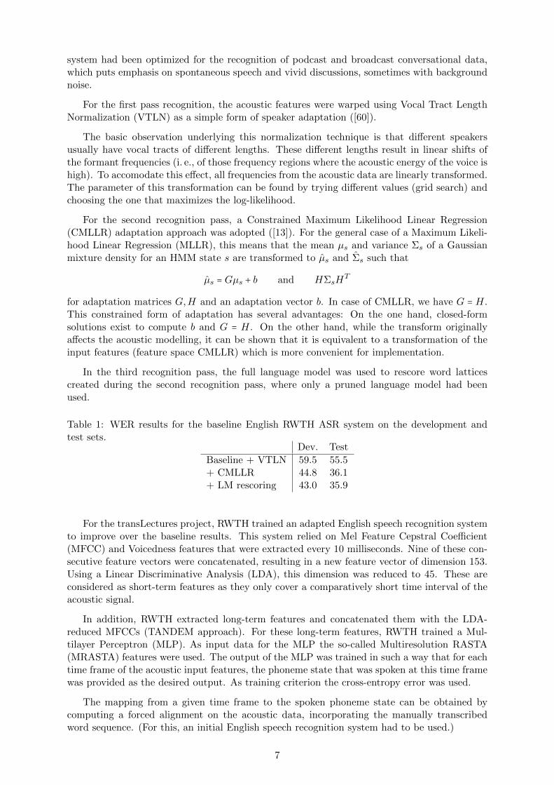
In the third recognition pass, the full language model was used to rescore word latticescreated during the second recognition pass, where only a pruned language model had beenused.

Table 1: WER results for the baseline English RWTH ASR system on the development andtest sets.

Dev. Test

Baseline + VTLN 59.5 55.5+ CMLLR 44.8 36.1+ LM rescoring 43.0 35.9

For the transLectures project, RWTH trained an adapted English speech recognition systemto improve over the baseline results. This system relied on Mel Feature Cepstral Coefficient(MFCC) and Voicedness features that were extracted every 10 milliseconds. Nine of these con-secutive feature vectors were concatenated, resulting in a new feature vector of dimension 153.Using a Linear Discriminative Analysis (LDA), this dimension was reduced to 45. These areconsidered as short-term features as they only cover a comparatively short time interval of theacoustic signal.

In addition, RWTH extracted long-term features and concatenated them with the LDA-reduced MFCCs (TANDEM approach). For these long-term features, RWTH trained a Mul-tilayer Perceptron (MLP). As input data for the MLP the so-called Multiresolution RASTA(MRASTA) features were used. The output of the MLP was trained in such a way that for eachtime frame of the acoustic input features, the phoneme state that was spoken at this time framewas provided as the desired output. As training criterion the cross-entropy error was used.

The mapping from a given time frame to the spoken phoneme state can be obtained bycomputing a forced alignment on the acoustic data, incorporating the manually transcribedword sequence. (For this, an initial English speech recognition system had to be used.)

7

RWTH used 268 hours of broadcast conversational data for training the MLP. A phonemeaccuracy of 57.9 % on cross-validation data was obtained. Instead of directly using the phonemeposterior probabilities (which corresponds to a vector of dimension 133 as there exist 133phoneme states in the training lexicon), RWTH extracted the corresponding activations ofa bottleneck layer directly preceding the output layer. This layer only has size 75. Thereforethis procedure can be interpreted as non-linear dimensionality reduction. More details on thetraining of MLP features can be found in [39].

In previous experiments, RWTH found that best results can be obtained when combining thisnon-linear dimensionality reduction with an additional linear dimensionality reduction, therebyreducing the dimension of the MLP features even further. Applying a Principal ComponentsAnalysis (PCA), the final dimension was set to 100.

For the acoustic model, 763 hours of manually transcribed speech data were used, including102 hours from the European Parliament Plenary Sessions (EPPS), the aforementioned Broad-cast Conversational (BC) data as well as 393 hours from the publically available HUB4 andTDT4 corpora (cf. Table 2).

Table 2: Acoustic training data for the RWTH English ASR system

Data source Duration Type

Quaero 268 h Broadcast Conversational data, podcastsEPPS 102 h European Parliament Plenary Session transcriptionsHub4 + TDT4 393 h Broadcast News data

Due to the fact that large amounts of training data available for the English language, atleast for acoustic training including the 20 hours of transcribed transLectures acoustic data didnot seem promising to RWTH. Instead, RWTH made use of the transLectures transcriptions forlanguage model training (see below). In addition, RWTH decided to include the EPPS data fortraining because they stem from a strongly related domain, and much more data are availablefrom this source.

A Gaussian Mixture Model (GMM) was trained on these data with a globally pooled diagonalcovariance matrix, resulting in a total of 1.2 million densities. The number of possible triphonestates was reduced to 4501 states by clustering using a Classification and Regression Tree(CART), see[64].

For the recognition lexicon, the phoneme set was based on the BEEP dictionary (whichis available from Cambridge University). The vocabulary included the most frequent 150,000words from the language model training data. As the language model data consist of a multi-tude of corpora having different sizes, the word frequencies were normalized over the availablecorpora.

Table 3: WER results for the improved English RWTH ASR system.

Dev. Test

Baseline + VTLN 44.5 34.0+ CMLLR 39.4 28.4+ LM rescoring 38.2 27.9

Table 3 states the current results of RWTH’s adapted English ASR system. Huge im-provements can be observed which are mainly caused by three different factors: Inclusion ofstate-of-the-art acoustic MLP features, adaptation to the lecture domain by including EPPSand BN data, and the incorporation of in-domain training data into the language model.

8

2.1.2 Slovenian lectures

RWTH’s phoneme set for the recognition of Slovene lectures is based on the one used in theLC-STAR project. In addition to 39 phonemes it contains one phoneme for silence, one forhesitation and one “garbage” phoneme for all kinds of noise. A grapheme-to-phoneme (G2P)model was trained on the LC-STAR lexicon (∼100k words) and used to create the traininglexicon.

The transcription of the training data was preprocessed as follows:

1. convert to lower case

2. collapse all types of hesitation tags to one

3. remove all other tags and punctuation marks

4. remove segments marked with ignore time segment in scoring

5. map incomplete words to [unknown]

6. use original spelling of foreign words

The acoustic training was performed on 34 lectures with a total duration of approx. 27 hoursof speech downsampled to 16 kHz. The initial Gaussian mixture model (GMM) with a globallypooled diagonal covariance matrix was trained on 33-dimensional features (16 MFCC plus firstorder derivative and first component of the second order derivative). The underlying HiddenMarkov model (HMM) has a three-state left-to-right topology and allows for loops and skips.Also across-word transitions are taken into account. The monophone system was trained withrespect to the maximum likelihood (ML) criterion by means of the Expectation Maximization(EM) algorithm. The number of Gaussians was increased in every iteration by splitting. Thebest alignment was then used for training of a triphone system. The number of triphone stateswas reduced to 4500 generalized states by tying with a Classification And Regression Tree(CART). The CART labels were used as classes to estimate an LDA transform that maps nineconsecutive MFCC feature vectors (four frames left and right context) to 45 dimensions. TheML training of the triphone system was performed on the LDA-transformed features, resultingin approx. 440k Gaussians.

Table 4: Corpus statistics

Corpus Number of lectures Duration [h]

train 34 27.0dev 4 3.1test 4 3.3

A second system was trained in the same fashion as the baseline system on the MFCCfeatures warped for Vocal tract length normalization (VTLN). The evaluation was performedon a development and a test set. The corpus statistics are given in Table 4. The results for thefirst two systems are given in Table 5.

During the recognition a 4-gram language model (LM) was used in all systems. See Section3.2 for details on language modeling. The recognition lexicon has been compiled from 400k wordsthat occur in all available text data most freqently. This way the ratio of out of vocabulary(OOV) words on the development set is approximately 2.4%.

9

Table 5: Recognition results (word error rates in %)

System Pass dev test

Baseline MFCC 1 38.8 59.2

(a) MFCC + VTLN 1 38.6 57.6(b) CMLLR in training 1 37.8 57.2(c) CMLLR in training+recognition 2 35.3 47.3

The transcription obtained from the first pass recognition was used for performing an unsu-pervised adaptation with CMLLR, aligning the features to the recognition output. The resultsof the second pass recognition performed on the CMLLR adapted features are given in Table 5.

While on the development data the relative improvement by CMLLR is in the usual range ofabout 10 %, the gain is much larger on the test data. This indicates a mismatch in the acousticconditions in the training and test data which is normalized by the CMLLR transform.

Such a mismatch also exists on the level of the language model, partly because of the widespectrum of topics covered in the lectures.

Moreover, the lecturers speak freely (“spontaneous speech” as opposed to “prepared” or“scripted”), while the language model is trained on written texts like books and articles. Lastly,Slovene is characterized by a large number of dialects, which makes the automatic transcriptionof lectures with many different speakers a difficult task.

2.1.3 Spanish lectures

The various sources of the audio training data are summarized in Table 6

Table 6: Audio data for transLectures Spanish ASR system

Data source No. of hours Type

transLectures 100 spontaneous, cleanQUAERO 170 News and podcasts, background noise/musicEPPS 90 Parliament speeches, cleanHub4 30 American Spanish

Some pre-processing steps are applied to all transcriptions; the numbers are expanded totheir word form, and for alternate terms (i.e. of the form /phrase 1/phrase 2//) the first termis retained.

The acoustic model training for the transLectures Spanish ASR system was done with theRWTH ASR software. The basic phoneme set consists of 31 language phonemes, plus onesilence and four non-language sound phonemes (representing noise, hesitation, articulation andbreath). The acoustic input features are three-layer Multilayer-Perceptron (MLP), which inturn have been trained on a concatenation of MFCC, PLP and Gammatone features. The 9output frames of the MLP are then concatenated together and then transformed by a lineardiscriminant analysis (LDA) transformation to 45 dimensions, and similarly transformed 45dimensional MFCC features are concatenated to it. The resulting 90 dimensional input featurevectors (with a resolution of 10 milliseconds per vector) are used as input features.

A previously trained QUAERO Spanish ASR system is used to generate an initial phoneme-to-feature-vector alignment for the audio data. The triphones are clustered into 4500 clas-sification and regression tree (CART) states. From this alignment, Gaussian mixture means

10

are estimated for each of these CART states (up to 256 Gaussian densities per state), and apooled diagonal covariance matrix. Using this newly calculated acoustic model, the phoneme-to-feature-vector alignments are refined. Speaker dependent constrained maximum likelihoodlinear regression (CMLLR) matrices are calculated for each speaker according to the speakerlabels as provided by the transcriptions. After adding these CMLLR matrices to the featureextraction pipeline, new Gaussian mixtures are estimated to the same resolution as before. TheGaussian mixtures are then converted to their log-linear parameter form λs and αs for an HMMstate s, so that the state posterior becomes

pΛ(st∣xt) =exp (λ⊺stxt + αst)

∑s′ exp (λ⊺s′xt + αs′)(1)

for a fixed alignment sT1 and acoustic observations xT1 . These new log-linear parameters arethen discriminatively trained according to the minimum phone error (MPE) objective function.Details of the Gaussian to log-linear conversion and the MPE optimization procedure can befound in [56]. The discriminative training resulted in about 1% absolute WER improvement onthe development and test data.

Table 7: WER (%) for transLectures Spanish

transLectures Corpus dev-2012 eval-2012

1st-pass 20.3 21.4with CMLLR 16.7 18.2with CMLLR (log-linear) 15.7 17.1

In addition to RWTH, UPVLC also investigated the adaptation of acoustic models for theSpanish poliMedia repository.

For this task, UPVLC focused on the development of a Spanish large-vocabulary ASR systemfor the poliMedia task. Specifically, UPVLC focused here on the development and adaptationof acoustic models, which have been modeled using Hidden Markov Models (HMMs). HMMshave been built using the AK toolkit [1]. This toolkit is released under a free software licenseand provides similar features to other HMM toolkits as HTK [63] or RASR [42]. However, inthis task UPVLC extended the AK features to support several widespread ASR techniques astriphone HMMs or cross-word recognition, as well as some adaptation techniques.

UPVLC has focused on transcriptions of the Spanish lectures from poliMedia. At the begin-ning of the project, 704 manually transcribed and segmented poliMedia lectures were providedfor the development of Spanish ASR systems. From these, 49 lectures where extracted to definedevelopment and test sets, leaving the rest of lectures for training purposes. Table 8 summarizesthe main statistics of the poliMedia speech database.

In order to develop Spanish acoustic models, training speech segments were first trans-formed into 16KHz, and then parameterized into sequences of 39-dimensional real feature vec-tors. In particular, every 10 milliseconds 12 Mel Frequency Cepstral Coefficients (MFCC), thelog-energy, and their first and second order time derivatives were calculated. Regarding thetranscriptions, 23 basic phonemes were considered plus a silence model. Words were trans-formed into phonemes according to the Spanish pronunciations rules. The resulting phonemetranscriptions also include speech disfluencies as hesitations, incorrect pronunciations, etc.

The previously extracted features were used to train a tied triphone HMM with Gaussianmixture models for emission probabilities. The training scheme is similar to the one describedin [63]. Firstly, each Spanish phoneme is modeled as a three state HMM with a conventional

11

Table 8: poliMedia Speech Corpus

Set Lectures Time (h) Phrases Running Words Vocabulary size

Train 655 96 41.5k 96.8k 28kDevelopment 26 3.5 1.4k 34k 4.5kTest 23 3 1.1k 28.7k 4k

Table 9: PPLs, OOVs (%) and WER (%) using several language models for the baseline SpanishASR system.

Language ModelDevelopment Test

PPL OOV WER PPL OOV WER

3-gram 298.0 4.5 36.4 317.6 5.2 36.24-gram 293.2 4.5 36.3 313.0 5.2 36.0

3-gram (External) 186.1 2.2 28.7 244.1 3.0 30.54-gram (External) 179.7 2.2 28.1 240.2 3.0 30.3

left to right topology. Secondly, these HMMs models are used to initialize triphones whichare extracted by modeling each phoneme with its context. Thirdly, an automatic tree-basedclustering based on manually crafted rules is used to tie the original states. As a product ofthe previous process, a tied triphone HMM with only one Gaussian component per state isobtained similarly to [64]. Finally, mixture components in each state are repeatedly split usingan iterative training process. During all training steps the Baum-Welch algorithm was used toestimate the model parameters that maximizes the log-likelihood for the input data [40, 63].In summary, UPVLC obtained 1745 HMM triphones with 3 342 tied-states having up to 64Gaussians per state. The training configuration was tuned on preliminary experiments usingthe development set.

In order to evaluate the trained acoustic models, UPVLC built n-gram language modelsusing the SRILM toolkit [52]. Two kinds of language models have been trained. The first ap-proach is a simple n-gram model trained only with the utterance transcriptions of the poliMediaspeech database. The second approach is fully described in Section 3.2.2 as the baseline. Insummary, this approach computes a linear mixture of language models trained with the poliMe-dia transcriptions along with other external resources described in Table 23, see Section 3.2.2for further information. For each case, UPVLC compared results for both 3-grams and 4-grams.In the case in which only poliMedia was used, the size of the vocabulary is about 28K, whereasfor the external data, the vocabulary was restricted to the 60K most frequent words. Regardingto the poliMedia transcriptions, UPVLC used what the speaker said instead of the correctedtranscription. Hesitations were considered a special word for the language model. Finally, thewell-known Viterbi algorithm was used to automatically recognize the videos. Recognition pa-rameters were tuned on development as for instance the grammar scale factor which was set to11, or the word insertion penalty, which was set to 0.

Table 9 reports WER results on development and test, for all the proposed language models.It is observed that when external text corpora is used a big improvement of about 6 points ofWER is obtained. The order of the language models slightly improves the WER when it isincreased from 3 to 4. The best result, 30.3%, is obtained with a 4-gram model.

Two speaker adaptation techniques were implemented in order to improve our best baselinemodel (4-gram language model with external data): fast Vocal Tract Length Normalization [60],and constrained MLLR (CMLLR) features [50, 16].

12

Table 10: WER (%) using several adaptation techniques on baseline Spanish ASR system.

Development Test

Baseline 28.1 30.3

VTN 26.2 28.8CMLLR (GMM-Diag.) 27.8 30.1CMLLR (HMM-Diag.) 27.3 29.7CMLLR (HMM-Full) 22.3 24.8CMLLR (HMM-Full 2nd Pass) 22.2 24.6

In order to apply the correct transformation, it is necessary to determine a suitable warpingfactor for each speech segment in training and recognition. In contrast to other methods, infast VTLN the selection of the warping factor during recognition is carried out without theneed of a preliminary transcription. Specifically, the selection is carried out using a Gaussianmixture model which is trained using the normalized training data [60]. In the recognitionprocess, UPVLC used a Gaussian mixture model of 128 components to select the optimalwarping factor, whereas, in the training process, our baseline HMM triphone model with onlyone Gaussian per state was used. In both training and recognition stages, the warping factorwas optimized at speech segment level. Results are shown in Table 10. As expected, the use offast VTLN outperforms our baseline model. In particular, UPVLC obtained a WER of 28.8%,1.5 points better than the baseline.

CMLLR is a technique for finding a linear transformation of the parameters of either aGaussian mixture model, or the Gaussian mixtures of a conventional HMM. This transformationis aimed at obtaining a data representation independent of the speaker.

In a first experiment, UPVLC compared two different target models: a mixture Gaussianof 512 mixture components (GMM), and our baseline triphone HMM with only one Gaussianper state. It is worth noting that in order to use a HMM as the target model for CMLLRa preliminary transcription is required. In our case, UPVLC used the transcriptions of thebaseline system. This first CMLLR experiment was carried out using diagonal transformationmatrices. UPVLC clustered each video in training and tested as a single CMLLR cluster withits own transformation. This decision was taken in light of poliMedia characteristics, since inmost of the poliMedia lectures there is only one speaker per video.

Results are shown in Table 10. In the GMM approach a small improvement of only 0.2 points(30.1%) over the test baseline was obtained. Similarly, for the HMM case UPVLC achieved animprovement of 0.6 points (29.7%). In both cases the improvement obtained was small, howeverthe HMM target model had a better performance.

A second experiment was carried out using full CMLLR transformation matrices instead ofdiagonal ones. Full CMLLR transformation matrices are more powerful than diagonal matricessince they can model covariances. The result, using the HMM target model, is also shown inTable 10. It is observed that for the case of full matrices, a much larger improvement is obtainedthan that of the diagonal case.

Finally, given the significant improvement obtained with full CMLLR (6 WER points),UPVLC performed a second pass with the transcriptions obtained by the previous CMLLRmodel. This second pass was performed with the expectation that improving the quality of thetranscriptions used to compute the transformation may improve the transformation itself. Afterthis new transformation is obtained, the same system is used to transcribe the videos again. Asit is observed in Table 10 the second pass obtains only a slight improvement yielding the bestresult of 24.6% WER points.

13

2.2 MAP adaptation of English lectures

2.2.1 Introduction

Acoustic adaptation has been investigated in two different scenarios, namely the supervisedadaptation of a general purpose acoustic model towards the lectures domain, and the unsuper-vised adaptation of a lectures specific acoustic model towards a particular lecture.

The first scenario is considered relevant for the rapid prototyping of initial models for thelectures domain which can help in further data collection and transcription efforts needed forthe development of improved models. The second scenario aims at the creation of high qualitymanuscripts for individual lectures. The investigations carried out in this direction focus onthe amount of data that is needed for adaptation and on a processing setup that foresees thedecoding of thousands of hours of lecture data.

The proper choice of an adaptation technique depends on the amount of adaptation datathat is available in a particular scenario. Maximum a posteriori (MAP) adaptation [15] is oneof the most efficient techniques if a large amount of data, say more than 10 – 15 minutes, isavailable.

The underlying principle of MAP adaptation is to consider the weighted log-likelihood func-tion FMAP

FMAP(λ) =T

∑t=1

log(pAM(xt∣λ)p(λ)),

where λ denotes the parameters of the acoustic model pAM (i. e., mean vectors and covariancematrices in case of a Gaussian mixture model). Here, xT1 denotes acoustic adaptation datato which an existing acoustic model shall be fitted. Under certain assumptions, closed-formsolutions exist to compute the adapted mean vectors and covariance matrices.

Originally developed for speaker adaptation, it has been successfully used for the adaptationof acoustic models towards particular dialects, languages, and/or acoustic conditions in the past.MAP is the method of choice for both cases described above, because in the transLecturesscenario one can safely assume the availability of a large adaptation corpus — a single lectureis usually much longer than the required 10 – 15 minutes. Moreover, its conceptual simplicityallows the rapid development of adaptation tools for the various acoustic models needed intoday’s multi-pass speech recognizers.

The EML transcription engine implements a two-pass recognition strategy that can alsobe found in several (open source) toolkits; see, for example, [43, 47]. After model basedspeech/silence segmentation, speaker independent, gender (or vocal tract length) normalizedacoustic models are used for the creation of a preliminary transcript in a first recognition pass.This transcript is used for the online computation of a speaker- specific affine feature transforma-tion that is required by the speaker adaptive acoustic models employed in a second recognitionpass. The second pass recognition results can be further improved, e.g. by a consensus networkalgorithm [28], or by word lattice rescoring, if processing time requirements permit.

Tools have been developed in the reporting period for MAP adaptation of the various modelsneeded in the recognition process sketched above:

� the (coarse, monophone) speaker independent acoustic models used for speech/silencesegmentation,

� the Bayesian classifier for text independent determination of a warping factor for vocaltract length normalization [61],

� the vocal tract length normalized acoustic models used in the first recognition pass,

14

Table 11: Properties of EML’s acoustic models used for massive adaptation.

EML English AMs lectures AM general purpose AM

training data (16 kHz) 100 hours 900 hoursHMMs (triphone context) 4000 40001st pass densities 680k 600k2nd pass densities 550k 430k

� the (coarse) acoustic model that serves as a target model in speaker adaptive training andrecognition [51], and

� the speaker adaptive acoustic models employed in the second recognition pass.

During development, special focus has been given to the integration of the adaptation toolsinto a (semi-)automatic workflow that allows the direct use of lecture transcripts produced bythe EML transcription platform for unsupervised adaptation, or the seamless use of manuallycorrected transcripts for (lightly) supervised adaptation. Another important aspect has beenthe integration of the developed tools into the acoustic model training environment used byEML’s language partners and customers for the development of acoustic models for severallanguages and/or target domains. Here, massive parallel processing is a key feature for therapid creation or adaptation of acoustic models from real application data.

2.2.2 Experimental Setup

Table 11 gives some details about the acoustic models for single pass and two pass recognitionemployed in our study. The lecture specific acoustic models are created from approximately 100hours of audio that were agreed upon for training in the transLectures consortium. In contrast,the general purpose acoustic models used in the supervised adaptation scenario are created froman EML in-house English speech data base available at EML. It consists of roughly 900 hoursof speech from many sources, but does not include any of the first models’ training data thatis of restricted (research only) use. Both acoustic models make use of the same 45-dimensionalfeature vector which results from the application of a linear discriminant analysis (LDA) to asliding window of 9 consecutive vectors consisting of 16 MFCCs and a voicing feature. TheMFCCs are computed in a vocal tract length normalized feature space that uses 13 warpingfactors in a range from 0.88 to 1.12. CMLLR is applied for the training of acoustic models forthe second decoding pass.

Both the lectures and the general purpose acoustic models use a single state HMM inventorythat consists of 4000 context dependent triphone HMMs. In both cases the HMMs are sharedbetween the acoustic models for the first and second decoding pass in order to provide a reason-able small memory footprint. Whereas model training originally aimed at the same number ofdensities in both cases, it turned out that the general purpose acoustic model performed betterwith fewer densities in both the first and second pass model.

The transLectures development set for the English language consists of audio from 4 lecturesfrom different speakers and serves as adaptation data for the supervised adaptation of the generalpurpose acoustic models. Both baseline and adapted models are tested against the transLecturestest set, which also consists of audio from 4 lectures. In case of the unsupervised adaptationtowards a particular lecture, different portions of the test set were used for the offline adaptationof the baseline models, see below. Finally, a “general English”, word based 4-gram languagemodel with a total of approximately 15 million n-grams was used in all experiments. No effortshave been made to adapt the language model towards the domains covered in the lectures dataused here.

15

Table 12: Supervised adaptation of a general purpose acoustic model; single pass recognitionword error rates for different adaptation weights.

General AM 1st-base 1st-5 1st-50 1st-100 1st-500

Lecture 1 63.3 62.8 61.9 62.0 63.3Lecture 2 35.8 35.6 35.5 35.4 36.8Lecture 3 50.3 50.2 49.9 49.4 52.6Lecture 4 48.3 48.2 48.0 48.3 49.0

Total 48.7 48.4 48.2 48.1 49.7

Table 13: Supervised adaptation of a general purpose acoustic model; word error rates for singleand two pass recognition.

General AM 1st-base 2nd-base 1st-100 2nd-100

Lecture 1 63.3 60.1 62.0 57.9Lecture 2 35.8 35.8 35.4 36.0Lecture 3 50.3 48.2 49.4 47.0Lecture 4 48.3 44.2 48.3 44.6

Total 48.7 46.1 48.1 45.6

2.2.3 Supervised Adaptation

Table 12 shows word error rates (different lectures from the transLectures English test set. Theoverall baseline WER is 48.7 percent; it reduces to 48.1 percent for the best adaptation weight(100) and increases to 49.7 percent, if too much weight is given to the adaptation data.

The best adaptation weight has also been used for the adaptation of the speaker adaptivemodels employed in the second recognition pass; results are given in Table 13.

It is worth noting that for the two lectures with lowest WER (Lecture 2 and Lecture 4)there is a small degradation when using the MAP adapted models for the second recognitionpass. However, a closer inspection shows that this degradation is due to an increased WER forsome background speakers, whereas results for the main speaker (lecturer) remain at least asgood as for the baseline models.

2.2.4 Unsupervised Adaptation

The unsupervised adaptation scenario aims at the rapid creation of the best possible transcriptfor a given lecture. The idea pursued in the experiments described here is to replace the standardtwo pass recognition strategy by a setup that collects some amount of adaptation data in anunsupervised manner, adapts the CMLLR models used in the second recognition pass, computesthe usual feature space transformation, and finally runs recognition with the adapted acousticCMLLR models. The interesting quantity in this setup is the amount of adaptation data: onthe one hand it should be as much as possible in order to achieve the best word error rate foreach show, on the other hand it should be as little as possible in order to guarantee a highthroughput if hundreds of lectures have to be transcribed.

Table 14 gives the baseline results for the transLectures test set and the lecture specificacoustic models, showing a baseline WER of 54.2 percent for single pass recognition and aWER of 47.9 percent for the two pass recognition setup. Note the degradation compared to thegeneral acoustic model above, which incorporates much more acoustic data.

16

Table 14: Baseline results (WER in percent) for the lecture specific acoustic models.

Lecture AM 1st-base 2nd-base

Lecture 1 63.4 53.9Lecture 2 37.8 36.2Lecture 3 50.2 44.8Lecture 4 62.5 54.2

Total 54.2 47.9

Table 15: Word error rates for adapted second pass (CMLLR) acoustic models (unsupervisedadaptation with different portions of the same lecture).

Lecture AM 2nd-base 2nd-10 2nd-25 2nd-50

Lecture 1 53.9 52.5 51.7 51.6Lecture 2 36.2 36.1 35.3 35.3Lecture 3 44.8 43.9 36.0 35.8Lecture 4 54.2 52.7 42.2 52.5

Total 47.9 47.3 40.6 45.3

Preliminary transcripts of different length have been created by decoding 10, 25, and 50percent of each lecture, corresponding to roughly 5, 12.5, and 25 minutes of audio. Segmentconfidence scores computed by the recognizer were then used for the selection of data for unsu-pervised adaptation. Following a rule of thumb, thresholds were set in a fashion that discardedthe 50 percent worst scoring segments of each (partial) lecture, resulting in a net amount ofroughly 2.5 – 12 minutes of audio data per lecture for adaptation. Finally, this data was used forboth MAP adaptation of the CMLLR models and the computation of a single speaker transformfor each lecture. Table 15 compares the word error rates for the standard two pass recognitionwith baseline acoustic models and single pass recognition with CMLLR-adapted models (usingdifferent amounts of adaptation data). While the degradation for Lecture 4 (2nd-50) deservesa closer examination, the sketched approach seems feasible. However, further implementationwork (dealing with the integration into the EML transcription platform) is needed in order tojudge the approach in terms of system throughput.

17

3 Massive adaptation of language models

3.1 Adaptation with in-domain data

During the recognition of the Slovenian lectures, RWTH used a 4-gram language model (LM) inall systems. The transcriptions of the acoustic training data have been interpolated with somefreely accessible texts collected on the web. The interpolation weights have been optimized onthe development set. The resulting perplexities on the development set are given in Table 16.

Table 16: Slovenian language model perplexities (lexicon size: 400k)

Text source, content Sentences Running words Perplexity (dev)

AM training data (lectures) 6.2k 136k 978Web data (books, articles) 1.5M 74.6M 518

Interpolated LM 1.6M 74.7M 468

For the Spanish lectures, various sources of language model text are summarized in Table17

Table 17: LM data for transLectures Spanish ASR system

Data source Running words

Translectures transcriptions 1MOther transcriptions 8MQUAERO 600MGigaword corpus 1000M

The language model is 5-gram with Kneser-Ney discounting to account for unknown n-grams. There are 320K words in the lexicon, with pronunciation variants for many frequentlyused words. The initial pronunciation model is based on a 60K-word lexicon for the TC-STARproject. A grapheme-to-phoneme (G2P) model trained on this initial lexicon is used to createthe pronunciations for those words which are present in the LM text but not in the initiallexicon. This works quite well in Spanish language, because the orthography to pronunciationrules are more consistent as compared to many other languages.

We use the measure of perplexity for adapting the language model. It is defined as theinverse probability indicating between how many different words the system chooses at everytime frame. The lower the perplexity the better. The formal definition is:

PPL = p(wN1 )−

1N = [

N

∏n=1

p(wn∣hn)]− 1

N

(2)

for a text wN1 of length N .

Table 18: Perplexity of development corpus

Data source ppl (dev-12)

Gigaword + QUAERO + old-transcriptions 274Gigaword + QUAERO + old-transcriptions + transLectures-transcription 195

18

As can be seen in Table 18, the perplexity of development corpus for the initial languagemodel (i.e. the one containing all the sources other than transLectures transcriptions) is signif-icantly reduced by adding the transLectures transcriptions. This is inspite of the fact that thesize of transLectures transcriptions data is tiny as compared to the other sources. Thereforewe can assume that adding more and more in-domain LM data will make the perplexity (andhence the WER) better. The OOV rate is 1.6%.

3.2 Adaptation based on lecture slides

3.2.1 English lectures

For the initial automatic transcription of the English video lectures a base language model wasused that is trained on transcribed lectures, subtitles, parliament speeches and general purposetext.

The video lecture repositories contain not only the recorded lecture but also correspondingslides. In Task 3.2 EML uses this additional information to adapt the language model. Theaccompanying slides for the lectures were extracted and preprocessed in Task 2.1. Furthermorerelevant material was downloaded from the web and preprocessed.

The EML English base language model was created from the text material as agreed onin the Scientific Evaluation Proposal and additional EML in-house data resulting in a corpusof about 350 million running words. Details on the composition of the corpus are shown inTable 19.

Table 19: English language model corpora

Corpus Sentences Running words

EPPS 52.477 780.616EuroParl corpus1 2.358.325 57.809.769JRC-Acquis corpus 3.839.309 60.985.421OPUS-OpenSubs 2.692.137 17.288.604TED 11.463 91.013VL lectures manually transcribed 13.641 143.044VL lectures with subtitles 364.597 2.069.683EML General Purpose Text 9.532.057 185.350.475EML Technical Texts and Lectures 1.509.503 21.434.875

Total 20.373.509 345.953.500

As baseline an EML-created general purpose vocabulary of 185.000 words was used. Thisvocabulary was enriched with the most frequent words with varying threshold from the abovementioned text material resulting in a total vocabulary of 235.000 words. The thresholds reflectthe relevance and reliability of the corpus.

One source of data for adaptation are the slides that accompany the lectures. We decided toonly use the material from ppt-slides, because the quality of text extracted from pdf- and jpg-slides is rather poor. Only in case there are no ppt-slides available for a specific lecture EML usedthe pdf-slides. Furthermore material was downloaded from the web by search requests aboutthe author, category and keywords of the lectures (described in Deliverable 2.1). Table 20 showsthe amount of data used for the adaptation experiments.

The base model is a 4-gram language model trained using modified Kneser-Ney smoothing.This model was adapted with the different corpora from Table 20 resulting in 10 adapted

19

Table 20: Adaptation Corpora

Material Sentences Running words

All material downloaded 1.307.616 22.454.212All available ppt-slides 427.557 3.554.763

All ppt-slides per categoryMaterial Sentences Running words

Mathematics 8.794 48.783Computers 14.666 103.700Business 33.180 212.738Society 29.184 157.125

ppt/pdf-slides per lectureMaterial Sentences Running words

webstart08 leitersdorf08 esvc (ppt) 234 1.122wict07 divjak deome (ppt) 563 3.979acs07 moulines mcm (pdf) 652 8.719apr08 culver aws (ppt) 201 962

Table 21: Results for the test and development set for adaptation with all material

Development setModel Perpl OOV (%) WER (%)

Baseline 632 0.65 60.6Adapt. with all ppt-slides 454 0.35 55.9Adapt. with all slides and downloads 421 0.21 55.1

Test setModel Perpl OOV (%) WER (%)

Baseline 395 0.45 46.0Adapt. with all slides 317 0.18 42.1Adapt. with all slides and downloads 308 0.15 42.1

language models. For each corpus the vocabulary was extracted and all unknown words occuringmore than once were added to the vocabulary. Subsequently a 4-gram language model wastrained from each corpus and linearly interpolated with the base model weighting the basemodel with 0.75 and the new model with 0.25.

Table 21 shows the baseline results and the results for the adaptation with all ppt-slides andfinally with all ppt-slides and the downloaded material.

Most of the benefit for WER, perplexity and OOV can be attributed to LM adaptationwith data extracted from the lecture accompanying slides, while the incorporation of more datadownloaded from the web has little or no effect.

Table 22 shows the baseline results, the results for the adaptation with all slides and down-loads (a), the results for the adaptation with the ppt-slides from all lectures with the samecategory (b) and with the ppt-slides from the specific lecture only (c).

For all but one lecture the adapation with all slides and downloaded material (a) givesslightly better results than the adaptation with the slides for the specific category (b).

As expected the lecture specific adaptation gives for 3 lectures the best results.

20

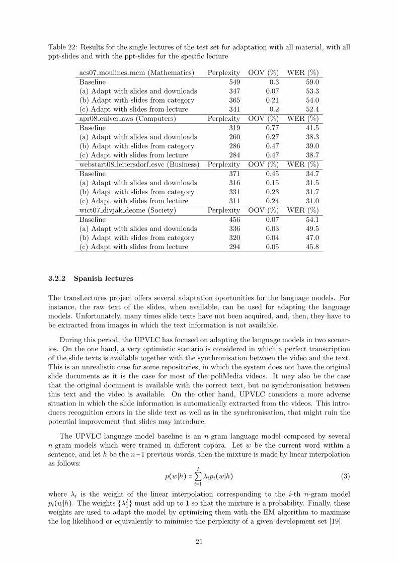
Table 22: Results for the single lectures of the test set for adaptation with all material, with allppt-slides and with the ppt-slides for the specific lecture

acs07 moulines mcm (Mathematics) Perplexity OOV (%) WER (%)

Baseline 549 0.3 59.0(a) Adapt with slides and downloads 347 0.07 53.3(b) Adapt with slides from category 365 0.21 54.0(c) Adapt with slides from lecture 341 0.2 52.4

apr08 culver aws (Computers) Perplexity OOV (%) WER (%)


webstart08 leitersdorf esvc (Business) Perplexity OOV (%) WER (%)


wict07 divjak deome (Society) Perplexity OOV (%) WER (%)


3.2.2 Spanish lectures

The transLectures project offers several adaptation oportunities for the language models. Forinstance, the raw text of the slides, when available, can be used for adapting the languagemodels. Unfortunately, many times slide texts have not been acquired, and, then, they have tobe extracted from images in which the text information is not available.

During this period, the UPVLC has focused on adapting the language models in two scenar-ios. On the one hand, a very optimistic scenario is considered in which a perfect transcriptionof the slide texts is available together with the synchronisation between the video and the text.This is an unrealistic case for some repositories, in which the system does not have the originalslide documents as it is the case for most of the poliMedia videos. It may also be the casethat the original document is available with the correct text, but no synchronisation betweenthis text and the video is available. On the other hand, UPVLC considers a more adversesituation in which the slide information is automatically extracted from the videos. This intro-duces recognition errors in the slide text as well as in the synchronisation, that might ruin thepotential improvement that slides may introduce.

The UPVLC language model baseline is an n-gram language model composed by severaln-gram models which were trained in different copora. Let w be the current word within asentence, and let h be the n−1 previous words, then the mixture is made by linear interpolationas follows:

p(w∣h) =I

∑i=1

λipi(w∣h) (3)

where λi is the weight of the linear interpolation corresponding to the i-th n-gram modelpi(w∣h). The weights {λI1} must add up to 1 so that the mixture is a probability. Finally, theseweights are used to adapt the model by optimising them with the EM algorithm to maximisethe log-likelihood or equivalently to minimise the perplexity of a given development set [19].

21

Table 23: Basic statistics of corpora used to generate the LM

Corpus Sentences Running words Vocabulary size

EPPS 132K 0.9M 27Knews-commentary 183K 4.6M 174KTED 316K 2.3M 133KUnitedNations 448K 10.8M 234KEuroparl-v7 2 123K 54.9M 439KEl Periodico 2 695K 45.4M 916Knews (07-11) 8 627K 217.2M 2 852KUnDoc 9 968K 318.0M 1 854K

Table 24: Basic statistics of poliMedia corpus.

Set Sentences Running words Vocabulary size

Train 41.5K 96.8K 28KDevelopment 1.4K 34K 4.5KTest 1.1K 28.7K 4K

Each individual language model was trained using the SRILM [52] toolkit in a differentcorpus. Table 23 summarises the main statistics of the used corpora. In addition, a languagemodel was trained from the Google counts corpus [31]. Finally, the poliMedia corpus wasalso used as the in-domain corpus, see details in Table 24. All n-gram models were smoothedwith modified Kneser-Ney absolute interpolation method [20]. The models used order 4, i.e. 4-grams, which were also pruned such that the perplexity increased by less than 2−10. Perplexitiesobtained for each of these individual models are reported in Table 25.

The baseline, as well as all further experiments have been conducted using the acousticmodel with CMLLR feature normalisation (full transformation matrices), which reports one ofthe best UPVLC results (see Table 10). More details on this acoustic model are given in theprevious Section 2.1.3.

Several experiments were carried out in order to assess the improvements that can be ob-tained with the text of slides in the poliMedia corpus (see Table 24). In all experiments, anadditional language model computed from the text of the slides was introduced in the linearmixture described in Equation (3). It is worth noting that this slide-dependent language modelvaries from one video to another. However, we optimised the linear interpolation weights for allthe n-gram models including the varying slide-dependent language model so that the perplexityis minimised on the poliMedia dev set.

As discussed above we considered two scenarios which were implemented by two sets ofslides transcriptions:

� human transcribed slides

� automatic transcription obtained with an OCR

In the first case, a human annotator transcribed the text of development and test slides so thatthey were perfectly synchronized as well as error free.

For the second case, automatic transcription were extracted from the videos in two steps.Firstly, each video was segmented into its corresponding slides by a very simple criterion. We

22

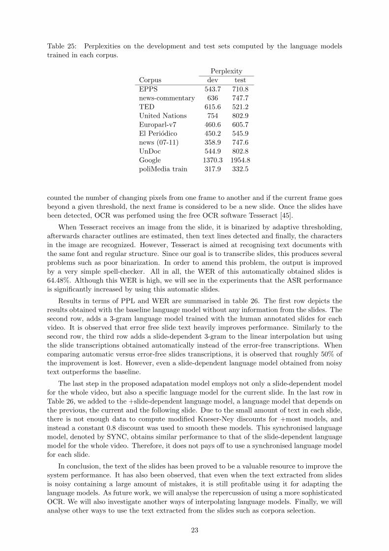
Table 25: Perplexities on the development and test sets computed by the language modelstrained in each corpus.

PerplexityCorpus dev test

EPPS 543.7 710.8news-commentary 636 747.7TED 615.6 521.2United Nations 754 802.9Europarl-v7 460.6 605.7El Periodico 450.2 545.9news (07-11) 358.9 747.6UnDoc 544.9 802.8Google 1370.3 1954.8poliMedia train 317.9 332.5

counted the number of changing pixels from one frame to another and if the current frame goesbeyond a given threshold, the next frame is considered to be a new slide. Once the slides havebeen detected, OCR was perfomed using the free OCR software Tesseract [45].

When Tesseract receives an image from the slide, it is binarized by adaptive thresholding,afterwards character outlines are estimated, then text lines detected and finally, the charactersin the image are recognized. However, Tesseract is aimed at recognising text documents withthe same font and regular structure. Since our goal is to transcribe slides, this produces severalproblems such as poor binarization. In order to amend this problem, the output is improvedby a very simple spell-checker. All in all, the WER of this automatically obtained slides is64.48%. Although this WER is high, we will see in the experiments that the ASR performanceis significantly increased by using this automatic slides.

Results in terms of PPL and WER are summarised in table 26. The first row depicts theresults obtained with the baseline language model without any information from the slides. Thesecond row, adds a 3-gram language model trained with the human annotated slides for eachvideo. It is observed that error free slide text heavily improves performance. Similarly to thesecond row, the third row adds a slide-dependent 3-gram to the linear interpolation but usingthe slide transcriptions obtained automatically instead of the error-free transcriptions. Whencomparing automatic versus error-free slides transcriptions, it is observed that roughly 50% ofthe improvement is lost. However, even a slide-dependent language model obtained from noisytext outperforms the baseline.

The last step in the proposed adapatation model employs not only a slide-dependent modelfor the whole video, but also a specific language model for the current slide. In the last row inTable 26, we added to the +slide-dependent language model, a language model that depends onthe previous, the current and the following slide. Due to the small amount of text in each slide,there is not enough data to compute modified Kneser-Ney discounts for +most models, andinstead a constant 0.8 discount was used to smooth these models. This synchronised languagemodel, denoted by SYNC, obtains similar performance to that of the slide-dependent languagemodel for the whole video. Therefore, it does not pays off to use a synchronised language modelfor each slide.

In conclusion, the text of the slides has been proved to be a valuable resource to improve thesystem performance. It has also been observed, that even when the text extracted from slidesis noisy containing a large amount of mistakes, it is still profitable using it for adapting thelanguage models. As future work, we will analyse the repercussion of using a more sophisticatedOCR. We will also investigate another ways of interpolating language models. Finally, we willanalyse other ways to use the text extracted from the slides such as corpora selection.

23

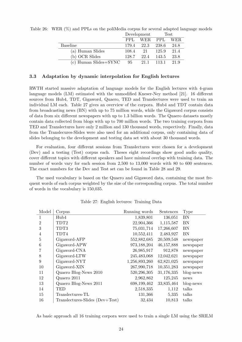
Table 26: WER (%) and PPLs on the poliMedia corpus for several adapted language modelsDevelopment TestPPL WER PPL WER

Baseline 179.4 22.3 238.6 24.8

(a) Human Slides 108.4 21 125.9 21.4(b) OCR Slides 128.7 22.4 143.5 23.8

(c) Human Slides+SYNC 95 21.1 113.1 21.9

3.3 Adaptation by dynamic interpolation for English lectures

RWTH started massive adaptation of language models for the English lectures with 4-gramlanguage models (LM) estimated with the unmodified Kneser-Ney method [21]. 16 differentsources from Hub4, TDT, Gigaword, Quaero, TED and Translectures were used to train anindividual LM each. Table 27 gives an overview of the corpora. Hub4 and TDT contain datafrom broadcasting news (BN) with up to 75 million words, while the Gigaword corpus consistsof data from six different newspapers with up to 1.3 billion words. The Quaero datasets mostlycontain data collected from blogs with up to 700 million words. The two training corpora fromTED and Translectures have only 2 million and 130 thousand words, respectively. Finally, datafrom the Translecures-Slides were also used for an additional corpus, only containing data ofslides belonging to the development and testing data set with about 30 thousand words.

For evaluation, four different sessions from Translectures were chosen for a development(Dev) and a testing (Test) corpus each. Theses eight recordings show good audio quality,cover different topics with different speakers and have minimal overlap with training data. Thenumber of words vary for each session from 2,500 to 13,000 words with 80 to 600 sentences.The exact numbers for the Dev and Test set can be found in Table 28 and 29.

The used vocabulary is based on the Quaero and Gigaword data, containing the most fre-quent words of each corpus weighted by the size of the corresponding corpus. The total numberof words in the vocabulary is 150,035.

Table 27: English lectures: Training Data

Model Corpus Running words Sentences Type

1 Hub4 1,839,801 136,051 BN2 TDT2 22,904,366 1,115,587 BN3 TDT3 75,031,714 17,266,607 BN4 TDT4 10,552,411 2,483,927 BN5 Gigaword-AFP 552,882,685 20,509,548 newspaper6 Gigaword-APW 973,188,204 46,157,888 newspaper7 Gigaword-CNA 26,985,917 912,878 newspaper8 Gigaword-LTW 245,483,068 12,042,621 newspaper9 Gigaword-NYT 1,256,893,260 62,821,025 newspaper10 Gigaword-XIN 267,990,718 10,351,283 newspaper11 Quaero Blog-News 2010 520,296,305 31,176,335 blog-news12 Quaero 2011 2,962,862 125,245 news13 Quaero Blog-News 2011 698,199,462 33,835,464 blog-news14 TED 2,518,335 1,112 talks15 Translectures-TL 131,366 5,335 talks16 Translectures-Slides (Dev+Test) 32,434 10,813 talks

As basic approach all 16 training corpora were used to train a single LM using the SRILM

24

Table 28: English lectures: Dev Data

Recording Material Running words Sentences

1 etvc08 barbaresco aoigt 5982 2582 mbc07 abdallah idt 8972 2933 sep09 jablonka eifd 9542 3644 slonano07 makovec spm 2442 83

Table 29: English lectures: Test Data

Recording Material Running words Sentences

1 acs07 moulines mcm 5886 1692 apr08 culver aws 12784 6103 webstart08 leitersdorf esvc 7555 2814 wict07 divjak deome 7330 262

toolkit [54]. The models were then tested on the Dev and Test data. For this purpose all fourtexts of each set were concatenated to one text and then evaluated for each LM.

The results are shown in Table 30. Mainly, the PPL ranges from 300 to 900 for the Dev setand from 200 to 700 for the Test set. Only the perplexity for the Translectures-Slides is veryhigh with over 1.000, which is not surprising, since it contains only few data.

Table 30: English lectures: Language model perplexities for single models

Model Dev Test

1 485.4 345.52 468.8 336.13 494.4 353.54 521.3 374.25 666.1 626.76 626.7 437.37 908.1 739.08 413.0 302.99 426.0 301.310 686.6 544.111 327.1 218.112 330.7 263.313 353.5 264.414 358.1 295.115 303.5 300.316 1140.1 1852.0

Next, the 16 language models were interpolated for the two concatenated evaluation corpora,which is named fixed interpolation. The interpolation weights were optimized on the Dev corpusand then also applied to the Test corpus with a resulting PPL of 138.8 and 132.2, respectively.Obviously, weighting down the worse language models leads to far better results than the bestsingle model. Additionally, the combination of multiple models offers better decisions for alln-grams, also lowering the perplexity.

For better adaptation interpolation was also carried out separately for each recording of the

25

Dev and Test set. The resulting perplexities were then combined to a single PPL, using thenumber of words per recordings as weighting factor.

This approach is named here as adapted interpolation and leads to small improvements of thePPL on both, Dev and Test set, down to 127.3 and 125.7, respectively. For better comparisonall interpolation results are shown in Table 31.

In later experiments the impact of the interpolation and adaptation shall also be measuredin terms of recognition error rates. For this purpose the language models have to be combinedto a single LM in a single file. The problem is that the data of all models are too much for suchan approach, since the calculation exceeds any memory capacity. Hence, RWTH chose to usejust the important LMs, meaning those with an interpolation weight above one percent. Theseare here the models 8, 9, 11, 12, 13, 14, 15 and 16, being two of the Gigaword corpora and allQuaero, the TED and the Translectures corpora. As shown in Table 31, a new interpolationwith these eight models leads to nearly the same results as an interpolation with all availablelanguage models.

As further modification, RWTH chose to use a background model to enhance PPL. The ideaof a background model is to concatenate all training corpora to a new additional corpora, whichis used to train a new language model. This model is then also included in the interpolationprocess for further improvement of the overall model. Again, due to memory limits it was notpossible to use all data for such a model. Since the calculation of a background model needs evenmore memory, RWTH was forced to further reduce the number of involved models. Hence, onlythe best models with an interpolation weight above ten percent were chosen, not considering themodel based on Translectures-Slides, since it holds to few data. This choice resulted in model11, 13, 14 and 15, the two Quaero Blog-News and again the TED and Translectures corporawithout slides. For completeness the interpolation results for those four models are also shownin Table 31.

After concatenating the data and calculating the background model it turned out that thismodel alone comes to a perplexity of 312.3 for the Dev set and 219.1 for the Test set, alsodepicted in Table 32. This is not surprising since the model contains all data without anyweighting and worse corpora with more text just outbalance better but smaller ones like theTranslectures corpora in this case. But combining the background model with the alreadychosen eight LMs slightly improves the overall perplexity nearly fully negating the effect of themissing eight language models.

Detailed results for this last combination are shown in Table 33. It should be noted thatfor the second and third recording of the Dev and the Test set very low perplexities from 116to 127 can be achieved.

As further research, RWTH plans the evaluation of cache language models as improvementof the shown adaptation approach. Furthermore, the generated language models will also betested in a speech recognition framework to verify the optimization of the perplexity in termsof word error rates.

26

Table 31: English lectures: Adaptation

Language Model

PerplexityDev Test

Interpolation InterpolationFixed Adapted Fixed Adapted

16 Models (all) 138.8 132.2 127.2 125.78 Models (Interpolation Weights Above 1%) 138.7 133.1 127.3 126.44 Models (Models 11 13 14 15) 173.2 170.2 141.0 139.7

8 Models + Background Model 138.5 132.2 127.0 125.8

Table 32: English lectures: Background model

Language ModelPPL

Dev Test

Background Model (Models 11 13 14 15) 312.3 219.1

4 Massive adaptation of translation models

4.1 Multi-domain translation model adaptation

4.1.1 Introduction

The performance of Statistical Machine Translation (SMT) models highly correlates with thedomain congruence between the corpora that were used to train the model on the one hand,and the test data that we are interested to translate on the other. For example, systemsthat were trained on large collections of parliamentary proceeding translations such as theEuroparl corpus [23], while achieving high BLEU scores on unseen test sentences from the samecollection, typically underperform when translating text from a different domain, such as newsstories or lecture transcriptions. However, while large in-domain bilingual training corpora area dependable ingredient of strongly performing SMT systems, we can hardly expect to haveaccess to such rare and expensive resources for every domain of interest.

A common solution to this problem explores the middle-ground between relying solely onlarge out-of-domain resources and only using small in-domain corpora. This involves traininglarge models from arrays of in- and out-of-domain data, producing translation systems whichcombine the wide coverage of large out-of-domain corpora, with the information on domain-specific translation correspondences contained in in-domain data. Straightforward methods tobring in- and out-of-domain training corpora together in SMT systems mostly perform betterthan employing exclusively one or the other kind of data. Still, such methods also involve thedanger of diluting the domain-specific translation correspondences contained in the in-domaincorpus with irrelevant out-of-domain ones. Also, when bringing all training data together, wemay end up with an incoherent translation model which while offering wide coverage, does notdo particularly well on any kind of data.

Previous work addressed these issues by tracking from which subset of the training dataeach translation option (e.g. a phrase-pair) was extracted, and using this information to bettertarget the translation of the in-domain data. [29] introduce sentence level features which registerfor each training sentence-pair the training corpus collection of origin and the language genreit belongs to. Using these features, they train a perceptron to compute a weight for eachsentence-pair, which is used to down-weight the impact during training of translation examples

27

Table 33: English lectures: Adaptation detailed

Recording Dev Test

PPL PPLInterpolation Interpolation

Words Fixed Adapted Words Fixed Adapted

1 5982 121.1 108.5 5886 150.0 152.02 8972 122.6 121.7 12784 118.3 116.43 9542 132.9 126.9 7555 125.5 118.24 2442 354.6 339.8 7330 127.6 132.1

all 26938 138.5 132.2 33555 127.0 125.8

that are not helpful on the test-set domain. [10] use similar collection and genre features todistinguish between training sentence-pairs and compute separate lexical translation smoothingfeatures [25] from the data falling under each collection and genre. Tuning on an in-domaindevelopment set allows to learn a preference for the lexical translation options found in thetraining examples which are similar in style and genre.

In this work, XEROX also focused on employing information on the origin of training pointsfrom particular subsets of a larger training set, which is sourced from a multitude of bilingualand monolingual data collections. We are particularly interested when such collections containdata of different linguistic styles or genres. In this multi-domain adaptation task, we aim tolearn translation models which bring together the translation correspondences found in eachtraining data subset, in such a way as to increase performance on the in-domain test data. Thedomain of interest for the trans Lectures project relates to transcriptions of video lectures fromthe scientific domain.

The first contribution of XEROX in this direction involves the introduction of additionaltranslation model features in a log-linear model. For every translation hypothesis formulatedduring decoding, these track the number of source words that got translated using a translationoption from each individual bilingual data collection of a large composite training corpus. Thisfollows the basic intuition that information on the origin of each translation option is usefulto distinguish those that are relevant to the domain of interest, which is also shared by worksuch as [29] and [10]. Contrary to previous work however, instead of indirectly employing thisinformation to assign training data weights or using it to train separate lexical translationmodels, we opt for directly monitoring and tuning the coverage of test sentences on the wordlevel by translation correspondences extracted from each training data collection.

The second contribution of XEROX is to complement a main Language Model (LM) trainedon all available composite target language data, with an array of Language Models, each of whichis only trained on target language data belonging to a particular training collection. The mainLM assigns a score related to the overall conformity of target language output to the lexicaland syntactic structure of the target language. In addition to this however, each additionaldomain-specific LM provides a measure of how close each candidate translation conforms tothe characteristics of the data belonging to each constituent training data collection of thecomposite training corpus. By weighing these scores log-linearly and tuning their weights on anin-domain development corpus, we aim to bias translation output towards effectively combiningthe domain-specific characteristics of each subset of the training material to match the test datadomain. In the empirical evidence we present below, we find that employing both approachesin tandem constitutes a robust framework to increase in-domain performance when training ondiverse sets of bilingual corpora, including data from the trans Lectures domain.

28

4.1.2 Baseline

While our method is directly applicable to hierarchical [9] and syntactically-driven SMT ap-proaches employing log-linear translation models, in the exposition and the experiments de-scribed below we will constrain ourselves to applying our approach on a Phrase-Based SMT(PBSMT) [25] baseline. In this section, we briefly discuss the main points of this family of SMTmodels.

A PBSMT model translates a source sentence by segmenting it into phrases and translatingeach phrase independently. To do so, it employs phrase-pairs extracted from word-alignedparallel corpora, which can be reordered during decoding. The conditional probability p(e∣f) ofeach translation hypothesis e to be the correct translation of the source sentence f is assessedby a log-linear combination of a number of Φ weighted features φ. Their weights λ are tunedon a small development corpus. During decoding, the translation e with the highest probabilityp(e∣f) according to the model is output.

e = arg maxe

p(e∣f) = arg maxe

log p(e∣f) (4)

log p(e∣f) =Φ

∑i=1

λi logφi(e, f) (5)

Typical features φ include conditional phrase and lexical translation probabilities, computedacross both translation directions (source to target, target to source), features tracking phrasereordering operations, as well as word and phrase generation penalties. Finally, the LanguageModel score φLM(e) assigned by an LM trained on target language monolingual data is alsoincluded as a crucial feature targeting the production of fluent target language output.

In the context of this part of the report, i.e. SMT systems trained on a composite corpuscombining multiple collections of training data, we will consider as our baseline a PBSMTsystem trained on the concatenation of all available bilingual and monolingual data, withoutregard to which collection each training example originates from. In this way, we end up with acompetitive baseline, which in typical applications combines the wide-coverage of larger out-of-domain corpora, with the domain-specific information contained in smaller corpora that have asmaller domain-divergence from the test data domain.

An often slightly more competitive baseline can be established by assigning a count higherthan one to sentence-pairs from in-domain training data collections. This assumes, however,that the target domain is known before training data is word-aligned, and that in-domaintraining data is available. We make no such assumptions in this work, allowing our method tobe applied to any test domain for which a small development corpus exists.

4.1.3 Lexical coverage features

The first extension of XEROX to the baseline involves the employment of additional lexicalcoverage features. These track during decoding how many source words get translated by usinga phrase-pair extracted from each collection of bilingual training data belonging in our overallcomposite training corpus.

Let us assume that we are training our model using a training corpus C composed as a setof a number of D constituent collections of training data Cd.

C =D

⋃d=1

Cd = {C1,C2, . . . ,CD} (6)

29

During phrase-pair extraction, we label each extracted pair ⟨e, f⟩ of source phrase f and

target phrase e, with a bit-vector b⟨e,f⟩ of length D. Each bit b⟨e,f⟩d is set to 1 if the related

phrase-pair can be extracted from the training data collection Cd, otherwise it is set to 0.

Multiple bits can be set to 1 in a single b⟨e,f⟩, as it is possible that a phrase-pair can beextracted from more than one training data collection Cd.

We consider that when a phrase-pair ⟨e, f⟩ with a source phrase e of length l is used in atranslation hypothesis, the training collection Cd that it was extracted from contributes l wordsin the translation of source sentence e. If ⟨e, f⟩ was extracted from a number n > 1 of collectionsCd, we consider that each such collection contributes l/n words.

Accordingly, our new lexical coverage features φdLC follow these assumptions to count howmany source words were covered using phrase-pairs extracted from each Cd. We add to themodel of equation (5), D additional features, one for each training data collection. Their valuesare computed for a translation f of source sentence e constructed using phrase pairs ⟨e, f⟩ asfollows.

logφdLC(⟨e, f⟩) =l ∗ b⟨e,f⟩d

∑Di=1 b

⟨e,f⟩i

(7)

logφdLC(e, f) = ∑⟨e,f⟩

logφdLC(⟨e, f⟩) (8)

4.1.4 Domain-specific language model array

Typical PBSMT systems employ a single Language Modelling feature φLM(e), which allows thedecoder to show a preference for output sentences which are fluent in the target language. ThisLM is commonly trained on all available target language resources, comprising of the target sideof the bilingual corpora Cd, together with any other available target monolingual resources.

However, when the monolingual training data are composed of a large array of individualcollections, each falling under a different language domain, the LM score provided by such afeature can: (a) be dominated by the style and genre of the larger data collections that providemore training examples, or (b) assign scores preferring a ‘lowest common denominator’ kind oflanguage use, promoting target output which favours general language use, but which cruciallyfails to match any style or genre in particular, including that of the test data domain.

In order to address these issues, XEROX trained individual Language Models from each tar-get monolingual data collection, and we used these LMs side-by-side with a main LM trained onall the available target data. Namely, if our target language corpus M consists of M collectionsof target sentences Mm, we train from each Mm a separate LM feature φmLM(e). We then addthese as additional Language Modelling features in the model of equation (5), not replacing butin addition to the main LM feature φLM(e).

For the total LM array ⟨φLM, φ1LM, . . . , φ

MLM⟩, we tune the feature weights ⟨λLM , λ1

LM , . . . , λMLM ⟩

together with the rest of the feature weights on a development set. This allows to set a pref-erence during decoding for the mixture of general language usage (as scored by φLM(e)) andparticular styles and genres (as scored by each φmLM(e)) that matches the test domain.

30

Table 34: Bilingual training data collections; size is measured in sentence-pairs

Corpus Genre Style Size

Europarl Parliament proceedings Formal speeches 1MJRC-Acquis Legal Formal text 1.2MWIT-3 Science for laymen Lectures 145KWMT-Newstext News Articles 137KCOSMAT Science for specialists Abstracts & Articles 56Ktrans Lectures Science for specialists Lectures 3.2K

Table 35: Single-domain and concatenated training data baselines, for the two test data domains

Test Domain Europarl JRC-Acq. WIT-3 WMT-News COSMAT trans Lectures Concat.trans Lectures 23.93 18.14 28.36 22.27 19.08 24.04 30.93WMT-News 24.47 20.50 22.38 24.05 15.23 11.02 28.20

4.1.5 Experiments

In order to empirically validate our method, we compiled a combined training corpus whichconsists of six distinct collections of bilingual training data between English and French, differingsubstantially in style and genre. Material includes content from the Europarl [23], JRC-Acquis[48], WIT-3 [7], 2011 WMT-Newstext [6], COSMAT [27] corpora, as well as the trans Lecturestraining corpus [58]. Table 34 lists the corpora and their key properties.

We experiment with two different domain adaptation scenarios, translating from English toFrench. Firstly, we explore translating transcriptions from the trans Lectures domain, wherea very limited in-domain corpus is available (3.2K sentence-pairs), in addition to 1K/1.3K de-velopment and test data respectively. Secondly, we also opt for the task of translating newstextfrom the WMT-Newstext domain, where a sizeable in-domain corpus exists (137K sentence-pairs), alongside a 2K development set and a 3K test set.

For our experiments, we choose for the Moses implementation of a PBSMT system [17] andkeep the default training and tuning parameters. We begin by building a series of single-domainbaselines, each trained solely on each individual training data collection. Language models foreach system are trained on the target side of each corpus and tuning of the feature weights isperformed with the MERT algorithm [32]. We also train a further baseline for each experimentalsetting, using the concatenation of all bilingual and monolingual data collections to train thetranslation and language model respectively.

Table 35 lists the BLEU scores achieved from each such system for the two translationtasks. The importance of in-domain training data is highlighted by the strong performanceof models trained on the in-domain corpora. Surprisingly, this applies even when trainingboth translation and language model only on the tiny trans Lectures training corpus of 3.2Ksentence-pairs. Still, larger corpora from more or less closely related domains (WIT-3 for thetrans Lectures task, Europarl for the ‘WMT-Newstext’ task) are able to score even higher thanthe more limited in-domain data, while the rest of the scores correlate with domain distance andcorpus size. Interestingly, the baseline training on the concatenation of all available resourcesoffers the most competitive performance, significantly outperforming all other single-domainsystems in both experimental settings.

We then experiment with extending the concatenated training data baseline with our lexicalcoverage (lexcov) and domain-specific LM (domain-lm) features. The six lexical coverage fea-

31

Table 36: Adapted models trained on multi-domain data collections. The ‘concatenated’ train-ing data baseline is compared to systems extending it with the additional lexical coverage(lexcov) and domain-specific LM (domain-lm) features. Scores with a (*) are significantlybetter than the best-scoring baseline at the 1% level. The best system(s) (if more than one,indistinguishable at the 1% significance level) are marked in bold.

Test Domain baseline lexcov domain-lm Tuning BLEU

trans Lectures

∎ MERT 30.93∎ MIRA 31.52∎ ∎ MIRA 32.36*∎ ∎ MIRA 32.48*∎ ∎ ∎ MIRA 32.44*

WMT-Newstext

∎ MERT 28.20∎ MIRA 28.04∎ ∎ MIRA 28.41*∎ ∎ MIRA 28.82*∎ ∎ ∎ MIRA 29.01*

tures (one for each training data collection) always complement the existing features of the base-line (conditional phrase and lexical translation probabilities, phrase penalty) in a phrase-tablewhich includes the same phrase-pairs as the baseline. Similarly, the array of six domain-specific5-gram LMs, smoothed using modified Kneser-Ney [8], complement as additional features theLM trained on the combination of all available target language data.

Table 36 lists the performance of our adapted models in comparison to the baseline system,where the latter does not include the features we introduced in Sections 4.1.3 and 4.1.4. For eachexperimental setting, we test one system which only extends the baseline phrase-table with thelexcov features, one which only introduces the domain-lm features and a third system whichcombines both kinds of features. We note that, although the baseline is already competitive inrelation to the single-domain systems, our systems which extend it with each of the two sets ofcontributed features further raise performance as measured by BLEU, with the improvementbeing statistically significant at the 1% level using the test of [22]. While both kinds of featurescontribute towards an in-domain performance improvement, combining them together managesto consistently deliver strong improvements across both test domains, with significantly higherBLEU than using each feature set on its own registered for the ‘WMT-Newstext’ task.

We must note that for our adapted systems, due to the large additional number of featuresthey employ, we opt for the Moses implementation of the MIRA algorithm [11] instead of MERTto tune the log-linear model weights. In order to make sure that the performance improvementdoes not follow solely from using a different tuning algorithm, we also tune a baseline sys-tem using the MIRA algorithm. Such a baseline actually registers a drop in performance forthe ‘WMT-Newstext’ task (28.04 BLEU) in comparison to using MERT for tuning. For thetrans Lectures task, the BLEU score of the MIRA-tuned baseline increases to 31.52 BLEU,still significantly surpassed by our best performing system by close to 1 BLEU.

4.1.6 Related work

Domain adaptation work for SMT models can be grouped in two categories. On the one hand,work such as [57, 4] aim to raise translation performance on in-domain test data by generatingadditional synthetic training data, using for example bootstrapping. On the contrary, ourapproach falls into a second category of SMT adaptation methods, which focus on employingmore efficiently the existing monolingual and bilingual training resources.

32

[29] exploit the information on the collections from which individual training examples orig-inate, as well as indications of genre that is sometimes present in training set metadata, tocompute a weight for each training sentence according to how helpful it is to translate datafrom the test domain. Our work is motivated by the same intuition, namely that we can bettertarget the test domain by exploiting the information on the grouping of composite, inhomoge-neous training data in more homogeneous data collections. However, previous methods try totune the desired contribution of each training collection in formulating translations hypothe-ses for the test domain indirectly, through computing importance weights for each trainingpoint [29], or training separate lexical translation models [10]. In contrast, we pursue the sameobjective with the much more direct lexical coverage features, achieving substantial empiricalimprovements over similar baselines as those considered by previous authors with a simpler toimplement method.

The concept of training separate language models from each training data collection insteadof a single model trained on all available data and using them as separate features duringdecoding, is not new. Still, previous work such as [44] explores the log-linear combination of avery small number (usually 2) of domain-specific LMs. In contrast, in this part of the report weexamine empirically the implications of employing large arrays of such domain-specific LMs intandem with an LM trained on all available data, and evaluate how these LM arrays complementthe simultaneous adaptation of the translation model.

Finally, recent work [12, 55] employs topic models to softly categorise composite trainingmaterial in more homogeneous collections, instead of using the human classification found incorpora metadata. We consider as an interesting direction for future work, to evaluate the use-fulness of such automatic clustering of training data as a replacement for the training collectionmembership information that we used in this work.

4.2 Adaptation using in-domain data

The Slovenian→English, English→Slovenian and English→German SMT systems are based onthe open-source toolkit Jane [59, 62]. For Slovenian→English and English→Slovenian, RWTHuses the phrase-based decoder, while for English→German the hierarchical phrase-based decoderis utilized.

RWTH used GIZA++ [36] to word-align the bilingual data, from which the phrase tableis extracted. The language models are 4-gram LMs trained with the SRILM toolkit [53]. Weuse the standard set of models with phrase translation probabilities and lexical smoothing inboth directions, word and phrase penalty and an n-gram target language model. The phrase-based system also includes a distance-based reordering model and three binary count features.The binary count features can have the values 1 or 0 and they indicate, whether the phrasepair appeared in the training data at least a certain number of times. Here, the features areassociated with the count values 1, 2 and 3. The log-linear parameter weights are optimizedwith MERT [35].

4.2.1 Slovenian↔English

RWTH used three different sources as training data, one large out-of-domain bilingual corpusand two small corpora containing translated video lectures. The baseline system is trained andoptimized on the JRC-Acquis corpus [49]. This corpus is composed of law texts and thereforenot related to the lecture domain. By adding training data collected from videoLectures.net

within trans Lectures and TED talks available for the IWSLT 2012 shared evaluation task(iwslt2012.org), results are substantially improved. Their strong impact can be explained bytheir relevance to the domain. The Slovenian language model is trained on the bilingual data

33

Table 37: Corpus statistics: Slovenian↔English.

Slovenian English

JRCSentences 1.09M

Run. Words 24.7M 27.5MVocabulary 199699 129335

JRC+TED+videoLecturesSentences 1.11M

Run. Words 25.2M 28.0MVocabulary 217731 136056

DevSentences 715

Running Words 15K 19KVocabulary 3428 2026

OOVs (run. words) 1418 772OOVs (run. words)+TED,videoLectures 1024 602

TestSentences 1360

Running Words 27K 37KVocabulary 4953 2832

OOVs (run. words) 1562 891OOVs (run. words)+TED,videoLectures 730 473

Table 38: Language model perplexities: Slovenian↔English.

Data ppl

SlovenianJRC 1397

+ TED + videoLectures 825

EnglishJRC + Europarl + News Commentary 657

+ TED + videoLectures bilingual 288+ TED + videoLectures monolingual 170

only. The English language model utilized additional sources, namely the Europarl and News-Commentary corpora provided for the WMT 2012 evaluation task (http://www.statmt.org/wmt12).For the Slovenian→English task, we finally added monolingual TED talk and textttvideoLec-tures.net data to train the language model, which again slightly improved the results. Bilingualdata statistics are given in Table 37, language model perplexities in Table 38. The trainingdata statistics for the final English language model can be found in Table 39. The results ofthe baseline translation systems are shown in Tables 40 and 41, and are measured in BLEU[%]and TER[%] on the development and test sets extracted from videoLectures.net.

Table 39: English language model training data, containing the JRC-Acquis, Europarl, News-Commentary, videolectures.net and TED corpora.

Sentences 3525055

Running Words 120389525

Vocabulary 427126

34

Table 40: Slovenian→English translation results.

SystemDevelopment TestBLEU TER BLEU TER

JRC 12.5 67.0 9.1 73.1+videoLectures & TED 20.5 61.8 15.0 67.8+TED monolingual 21.6 59.5 15.7 65.2

Table 41: English→Slovenian translation results.


JRC 7.7 79.9 6.2 95.0+ videoLectures & TED 13.4 68.5 12.0 77.4

4.2.2 English→German

For the English→German translation system, in addition to the 4,019 bilingual training sen-tences collected from videoLectures.net, we used the bilingual TED talk data, which addedan additional 129 911 bilingual training sentences. The corpus statistics can be found in Table43. The German language model is trained on the target side of this data and has a perplexityof 191. It is further improved by utilizing the slide content which is available for the lectures.This is described in the following Section.

Unfortunatelly, due to the tight schedule of the scientific evaluation procedure, both forEnglish→Slovenian and English→German the systems used for evaluation are inferior to theones described here. Therefore, we expect strong improvements in the next quality control.

4.3 Adaptation using slides

We focused on using the slide text as an additional source of information for massive adaptation.

4.3.1 Extracting the slide text

In addition to the transcribed and translated sentences, the slides shown during the lecturesare also given. All slides are available in the jpeg format, and most of them also as pdf and/orpowerpoint presentation. We extracted the textual information from the pdfs using the opensource pdftotext tool. The powerpoint presentations could be processed as well by convertingthem into pdf files first. One lecture provided only the jpeg images of the slides. As theresolution of the jpegs was rather small, we manually transcribed these few slides instead ofusing an OCR software to ensure a good data quality.

We aligned the spoken sentences with the slides using the time stamps given in the xml data.Since the alignment information between the images and the extracted text was not provided,we relied on the assumption that each new shown slide was in fact the next slide given in thepdf. This procedure led to a parallel corpus consisting of three parts, the English sentence, itsGerman translation and the text of the slide shown while the sentence was spoken.

35

4.3.2 Discriminative word lexica

We apply a discriminative word lexicon to incorporate the slide information into a statisticalmachine translation system. Discriminative word lexica (DWL) as proposed in [30] model theprobability of the presence or absence of words in the target sentence based on the presenceof words in the source sentence. In our scenario, we use the content of the slide as the sourceinformation and want to predict the presence or absence of words in the target sentence. Asthe spoken sentences are usually longer than the brief information presentented on the slides,regular translation models such as phrase models are not suitable, because many spoken wordsare not contained on the slides, and the words on the slides might be spread throughout thespoken text. The discriminative word lexicon on the other hand does not take into account theorder in which the words appear and thus can be applied to this scenario. Instead of modelingphrases or sequences, the DWL only models the bag of words of the target sentence given thebag of words of the slide. Formally speaking, given the words on the slides, g1, g2, ..., gJ = gJ1and the target sentence e1, e2, ..., eI = eI1, the discriminative word lexicon models the probabilityof the bag of words {eI1} made up of words from the vocabulary Ve:

P ({eI1}∣{gJ1 }) = ∏e∈eI1

P+(e∣{gJ1 }) × ∏e∉eI1

P−(e∣{gJ1 }) (9)

Here, the two probabilities P+ and P− are modeled as log-linear models:

P+/−(e∣{gJ1 }) =exp(∑g∈gJ1

λ+/−g,e )

exp(∑g∈gJ1λ+g,e) + exp(∑g∈gJ1

λ−g,e)(10)

The DWL is trained on the slide information and the target sentences of the training data.In decoding, we combine the DWL model with other regular translation models in a log-linearframework and extend our decoder to use both the source sentence and the slide informationas input information.

As the slides of the lectures contain a lot of mathematical symbols and formulas as wellas numbers, we tested two scenarios, one using all possible words, and one using only wordscontaining letters from the alphabet, thus excluding numbers and formulas. It turned out thatthe latter scenario led to a better translation performance. It seems that the key words on theslides triggered the translation of certain target phrases and formulations.

4.3.3 Adaptation using a recurrent neural network

As an alternative approach for utilizing the additional information given in the slides, RWTHtrained recurrent neural network (RNN). The RNN structure is closely related with MultilayerPerceptrons (MLP) [41, 5], but the output of one or more hidden layers is reused as additionalinputs for the network in the next time step. This structure allows the RNN to learn wholesequences without restricting itself to a fixed input window. The long short-term memory(LSTM) [18] is applied to counter the effect that long distance dependencies are hard to learnwith gradient descent. This is often referred to as vanishing gradient problem [3].

The input layer of the recurrent neural represents the previous word in the target language,the aligned words in the source language, and all words that are shown on the current slide.The size of the input layer is therefore the input vocabulary + the output vocabulary + theslide vocabulary. In each step, all input nodes are inactive, except for the node representingthe previous word, all aligned words and all words on the current slide. The RNN uses theseinputs to predict the next word and calculate a score for the whole sentence using a softmaxlayer similar to the application of neural networks to language modeling [2]. This additional

36

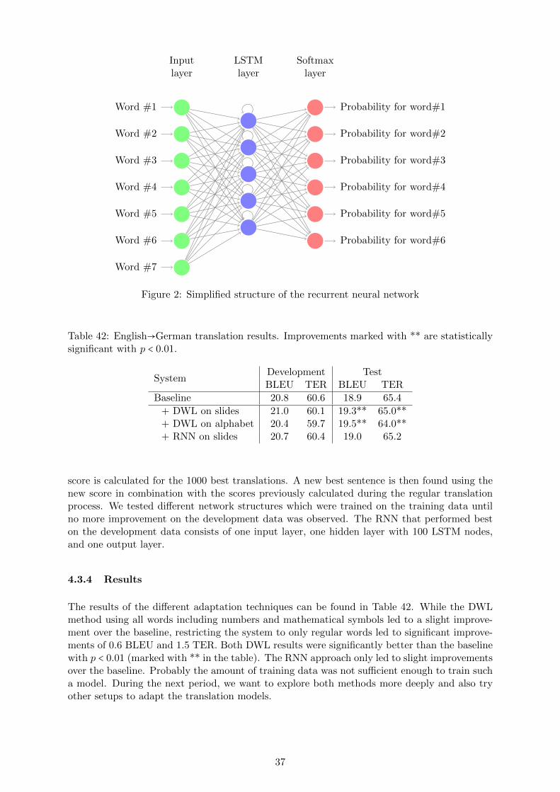
Word #1

Word #2

Word #3

Word #4

Word #5

Word #6

Word #7

Probability for word#1






LSTMlayer

Inputlayer

Softmaxlayer

Figure 2: Simplified structure of the recurrent neural network

Table 42: English→German translation results. Improvements marked with ** are statisticallysignificant with p < 0.01.


Baseline 20.8 60.6 18.9 65.4

+ DWL on slides 21.0 60.1 19.3** 65.0**+ DWL on alphabet 20.4 59.7 19.5** 64.0**+ RNN on slides 20.7 60.4 19.0 65.2

score is calculated for the 1000 best translations. A new best sentence is then found using thenew score in combination with the scores previously calculated during the regular translationprocess. We tested different network structures which were trained on the training data untilno more improvement on the development data was observed. The RNN that performed beston the development data consists of one input layer, one hidden layer with 100 LSTM nodes,and one output layer.

4.3.4 Results

The results of the different adaptation techniques can be found in Table 42. While the DWLmethod using all words including numbers and mathematical symbols led to a slight improve-ment over the baseline, restricting the system to only regular words led to significant improve-ments of 0.6 BLEU and 1.5 TER. Both DWL results were significantly better than the baselinewith p < 0.01 (marked with ** in the table). The RNN approach only led to slight improvementsover the baseline. Probably the amount of training data was not sufficient enough to train sucha model. During the next period, we want to explore both methods more deeply and also tryother setups to adapt the translation models.

37

Table 43: Corpus Statistics English → German

English German

Train

Sentences 4019Running Words 103306 96627

Running Words without Punct. Marks 92709 83457Vocabulary 5930 9191Singletons 2491 4906

Train + TED


Running Words without Punct. Marks 2288376 2162976Vocabulary 45479 69522Singletons 18043 31877

Dev


Running Words without Punct. Marks 26151 23254Vocabulary 2701 3762

OOVs (running words) 2210 2930+TED 711 1533

OOVs (in voc.) 1027 1761+TED 350 886

Test


Running Words without Punct. Marks 32590 27649Vocabulary 2836 4140

OOVs (running words) 2309 3231+TED 483 1483

OOVs (in voc.) 985 1973+TED 242 937

4.4 Sentence selection

Among the trans Lectures tasks, obtaining automatic translations of educational videos is oneof the most challenging tasks, since for many of the language pairs used in the project thereare large amounts of external data available. For instance, there are several parallel corpora forSpanish and English such as the Europarl-v7. However, the domain of these external corporasignificantly differs from that of the the educational lecture domain. The objective of this task isto use lecture-specific knowledge in order to adapt the translation models to the lecture domain.

Most recent literature defines the Statistical Machine Translation (SMT) problem [37, 33],as follows: given an input sentence f from a source language, the purpose of SMT is to find itstranslation e in a target language such that

e = arg maxe

K

∑k=1

λkhk(f, e) (11)

where hk(f, e) denotes the so-called feature functions, and λk are their corresponding weightsin the log-linear mixture. The feature functions model important factors for the translation off into e, as for instance the target language model, the reordering models or several translationmodels.

Consequently, the problem of adapting an SMT model can be reformulated as adapting eachof the individual features that compose the model. In this task, UPVLC has focused on the

38

adaptation of the language models, and the translation models in the context of SMT. In orderto adapt the models to the domain of transcribed video lectures, the following techniques wereapplied:

1. A big language model was trained and adapted from several monolingual corpora similarlyto Task 3.2 (see section 3.2.2).

2. A successful sentence selection technique was applied to obtain a representative corpusfor the transcriptions to be translated.

3. The language model trained at step 1 is introduced into the model computed at step 2 asa feature function.

Similarly to Section 3.2.2, the big language models were obtained by linearly mixing severaln-gram language models trained in different corpora. Let w be the current word within a tran-scription, and let h be the n−1 previous words, then the mixture is made by linear interpolatingthe language models as follows

p(w∣h) =I

∑i=1

λipi(w∣h) (12)

where λi is the weight of the linear interpolation corresponding to the i-th n-gram modelpi(w∣h). The weights {λI1} must add up to 1 so that the mixture is a probability. Finally, theseweights are used to adapt the model by optimizing them with the EM algorithm to maximizethe log-likelihood or equivalently to minimize the perplexity of a given development set [19].

As discussed above, there are many external bilingual corpora for training SMT systems.The main adversity when attempting to exploit such corpora is that there are considerabledifferences between their domains and the project domain. For instance, while in the trans Lec-tures case, the corpus to be translated are transcriptions of video lectures, one of the externalcorpora domain is parliamentary proceedings of the United Nations. Bilingual sentence selec-tion techniques aim at selecting a subset of the available bilingual data with which to traina SMT system. This selection is performed to maximize performance, and then these tech-niques can play the role of domain adaptation techniques if used properly. In addition, as aside-effect, these techniques dramatically amend another problem related to huge amounts ofexternal corpora, i.e. the high computational cost required to work with large amounts of data.

UPVLC has worked with a successful sentence selection technique called infrequent n-gramrecovery [14]. This technique selects the minimal set of sentences that yield reliable estimationsfor all the n-grams that occur in the text to be translated. An n-gram is considered frequent,and consequently reliably estimated, if it occurs more than t times in the selected trainingdata. In the case of adaptation, in which typically there is a small in-domain training corpus,the occurrences into the in-domain corpus are considered when deciding whether a n-gram isfrequent or infrequent. For selecting, all the sentences in the external corpora are scored asfollows

i(f) =∑w∈X

min(1,N(w))max(0, t−C(w)) (13)

where X is the set of n-grams that appear in the sentences to be translated and w one of them;C(w) the counts of w in the source language training set; and N(w) the counts of w in thesource sentence f to be scored. Note that the score i(f) gives higher weight to the n-gramsmost infrequent n-grams in the training set. The scored sentences are then selected one by oneupdating the counts of the n-grams in the training set together with the scores of the externalcorpora sentences after each selection. The process is stopped whenever a maximum number ofsentences is obtained, or no infrequent n-ngram is left in the training corpora [14].

In order to combine the large adapted language models from step 1 together with the modeltrained in a corpora selected with bilingual sentence selection techniques, a log-linear interpola-tion is performed [26]. This log-linear interpolation is implemented in many statistical machinetranslation toolkits as for example Moses [24].

39

Table 44: Basic statistics of the external corpora involved in the generation of the Spanish LM

Corpus Number sentences Number of words Vocabulary size

EPPS 132K 0.9M 27KNews Commentary (Es) 183K 4.6M 174KTED (Es) 316K 2.3M 133KEuroparl v7 (Es) 2 123K 54.9M 439KEl Periodico 2 695K 45.4M 916KNews (07-11) (Es) 8 627K 217.2M 2 852KUnited Nations (Es) 9 493K 253M 1 643KUnDoc (Es) 9 968K 318.0M 1 854K

Table 45: Basic statistics of the external corpora involved in the generation of the english LM

Corpus Number of sentences Number of words Vocabulary size

TED (En) 142K 2.3M 100KNew Commentary (En) 208K 4.5M 150KEuroparl v7 (En) 2 218K 54.1M 326KUnited Nations (En) 10 593K 286M 1 835K109 (En) 19 842K 504.8M 5 834KNews (07-11) (En) 48 872K 986M 6 169K

4.4.1 Experiments

In this section, we describe the experiments carried out by the UPVLC in order to assess theperformance of the proposed massive adaptation techniques. For reporting performance, weused BLEU [38] and TER [46]. It is worth highlighting that while BLEU is a precision metric(the higher, the better), TER is an error metric (the lower, the better). All the experimentsuse Moses [24] as the translation engine. The word alignments needed by Moses are computedusing GIZA++ [34]. Finally, the n-gram language models were computed using the SRILMtoolkit [52].

The experiments were carried out in two trans Lectures corpora: poliMedia from Spanish toEnglish (Es→En) and VideoLectures.NET from English to Spanish (En→Es). The TED corpus,which is composed of educational talks, was used as additional in domain corpus. The mainstatistics of training, development and test sets of the in-domain corpora are shown in Table 46.As external out of domain corpora for the bilingual selection, we used Europarl and UnitedNations corpora. Table 47 summarizes the most important statistics of these corpora. It mustbe noted that, after selecting the sentence from the external corpora, the in-domain trainingcorpora is added to them in order to create the final training set.

Regarding the large language models, since two directions were considered, we computed twoexternal language models: one for Spanish, and another for English. In both cases and in orderto compute the individual language models, we used several bilingual and monolingual externalcorpora in addition to Google counts [31] and the in-domain corpora. Prior to the computationof individual language models, all the corpora were cleaned in order to avoid having noise orvery short sentences. Tables 44 and 45 summarize the most important statistics of the externalcorpora once they have been cleaned. Each individual language model was trained using theSRILM [52] toolkit in a different corpora. All n-gram models were smoothed with modifiedKneser-Ney absolute interpolation method [20]. The models used order 4 and were interpolatedto minimize the perplexity of the in-domain development set [19].

40

Table 46: Main figures of the in domain corpora.

Corpus SentencesWords Vocabulary

en es en es

TED 144K 2.6M 2.45M 46.4K 67.9K

VideoLectures.NET training 2142 58K 54.2K 3.74K 5.04KVideoLectures.NET development 1013 28.6K 27.4K 6.23K 2.7K

VideoLectures.NET test 1360 36.1K 33.5K 6.23K 3.3K

poliMedia training 1529 40.2K 40.3K 3.86K 4.71KpoliMedia development 1401 38.7K 37.8K 3.66K 3.51K

poliMedia test 1139 32.1K 32.1K 3.26K 4.08K

Table 47: Main figures of the corpora from which the sentences are selected.

Corpus SentencesWords Vocabulary

en es en es

Europarl 1.73M 40.6M 42.3M 98.4K 149KUN 11M 298M 340M 55.6K 57.1K

Table 48 summarizes the adaptation results obtained for the spanish to/from english trans-lation. For computing the baseline, we used the in-domain training set and the Europarl corpusin order to train the translation and language models. The baseline language model is 5-grammodel smoothed with modified Kneser-Ney absolute interpolation method [20]. For the base-line a result of 30.9 and 23.4 BLEU points were obtained for Es→En and En→Es, respectively.This figures were slightly improved by using the linearly interpolated language model insteadof the baseline language model. A significant improvement is obtained by bilingual sentencesselection techniques. This improvement is even larger with the linearly interpolated languagemodel. However, the best results were obtained by a log-linear combination of both languagemodels: the large linear mixture and the language model resulting from sentence selection. Thefinal improvement after adaptation score a total of 33.5 and 26.0 BLEU points for Es→En andEn→Es, respectively.

In summary, the three proposed techniques have successfully adapted the system. Actually,the best result was obtained by means of the combination of all three of them. In addition, asa byproduct of the bilingual sentence selection, the selected corpus was reduced to just 1.5% ofthe total available data, which significantly reduces the computation requirements for trainingthe statistical translation system.

Table 48: Results in BLEU and TER in the test set of poliMedia and VideoLectures.NET

VideoLectures.NET poliMediaBLEU TER BLEU TER

Baseline 30.9 48.7 23.4 56.5+linear interpolation 31.2 48.7 24.0 56.4

Selection 32.4 47.2 24.9 55.6+linear interpolation 33.3 46.4 25.3 55.1+log-linear interpolation 33.5 46.1 26.0 54.6

41

5 Conclusion

In this report, for each of the three languages and six language pairs, we documented thetraining of our baseline systems. These systems will form the basis for future adaptation exper-iments, and their continuous improvement will depict the progress of adaptation methods whenevaluated on the test data as well as on the full videoLectures.net and poliMedia repositories.

Regarding acoustic adaption, we observed that large improvements in word error rate canbe obtained when using CMLLR adaptation. For some of the languages, especially Slovene, wefound that the improvements incurred by CMLLR are much larger than what can usually beexpected from this technique. In addition, the number of different speakers in lecture record-ings usually is very small. This may provide experimental evidence that not only the speakervariation is normalized by this transformation but also the acoustic conditions.

In a second set of experiments, we analyzed the effects of MAP adaptation. We distinguisheda supervised versus an unsupervised setting. For the supervised case, a given acoustic model wasadapted towards the lecture domain using all available acoustic in-domain data and its manualtranscriptions. For the unsupervised case, the baseline acoustic model was adapted with varyingamounts of audio data of a specific lecture, and only the recognized word sequence for this lecturewas used. Considerable improvements were achieved with supervised MAP adaptation, even ontop of a CMLLR adaptation, and even larger gains were obtained for unsupervised adaptation.

For language model adaptation, we investigated several variants of interpolation. It wasfound that the use of the text data extracted from the slides accompanying a specific lecturewas of great benefit for the recognition quality. This was verified by all partners participatingin task 3.2.

The slides were not available for each lecture in a format where the text could be directlyextracted. As an alternative, by using OCR technology the text data were obtained from imagefiles depicting the slides. Even though the error rates of the OCR system were comparativelyhigh for this task, the language model adaptation based on the OCR texts still gave significationimprovements, although these are still much lower than those for the correct slide texts.

For the adaptation of translation models, discriminative word lexica provided a significantimprovement in translation quality. Recurrent neural networks so far only gave minor benefits,and we plan to extend our work along this direction in the future. Sentence selection helpedto improve translation systems considerably. We observed the largest gains in BLEU when thistechnique was not only limited to the translation model but was extended to selecting trainingdata for the language model, too.

We also examined how we can increase in-domain translation performance when trainingon composite SMT training data. We proposed two adaptation methods, one targeting thetranslation model and one focusing on the language modeling component of phrase-based sys-tems. We used information on the membership of training examples in training data collectionsto better combine together translation options extracted from each collection during decoding.We also examined the use of an array of domain-specific language models to learn a blend ofthe individual genre and style of each collection, which matches more closely the test data do-main. Our empirical evaluation promotes the combination of the two methods as an effectiveand easy to implement method to raise in-domain performance when training on multi-domaincorpora, and demonstrated that our methods deliver a significant performance improvementwhen translating scientific video lecture transcriptions for the trans Lectures project.

42

References

[1] AK toolkit. http://aktoolkit.sourceforge.net/.

[2] Y. Bengio, H. Schwenk, J.S. Senecal, F. Morin, and J.L. Gauvain. Neural probabilisticlanguage models. Innovations in Machine Learning, pages 137–186, 2006.

[3] Y. Bengio, P. Simard, and P. Frasconi. Learning long-term dependencies with gradientdescent is difficult. IEEE transactions on neural networks / a publication of the IEEENeural Networks Council, 5(2):157–166, March 1994.

[4] Nicola Bertoldi and Marcello Federico. Domain Adaptation for Statistical Machine Trans-lation with Monolingual Resources. In Proceedings of the Fourth Workshop on StatisticalMachine Translation, pages 182–189, Athens, Greece, 2009. Association for ComputationalLinguistics.

[5] Christopher M. Bishop. Neural Networks for Pattern Recognition. Oxford University Press,USA, 1 edition, January 1996.

[6] Chris Callison-Burch, Philipp Koehn, Christof Monz, and Omar Zaidan. Findings of the2011 Workshop on Statistical Machine Translation. In Proceedings of the Sixth Workshop onStatistical Machine Translation, pages 22–64, Edinburgh, Scotland, July 2011. Associationfor Computational Linguistics.

[7] Mauro Cettolo, Christian Girardi, and Marcello Federico. WIT3: Web Inventory of Tran-scribed and Translated Talks. In Proceedings of the 16th Conference of the EuropeanAssociation for Machine Translation (EAMT 2012), pages 261–268, Trento, Italy, May2012.

[8] Stanley F. Chen and Joshua Goodman. An Empirical Study of Smoothing Techniques forLanguage Modeling. Computer Speech & Language, 13(4):359–393, 1999.

[9] David Chiang. A Hierarchical Phrase-Based Model for Statistical Machine Translation. InProceedings of the 43rd Annual Meeting of the Association for Computational Linguistics(ACL’ 05), pages 263–270, Ann Arbor, Michigan, June 2005.

[10] David Chiang, Steve DeNeefe, and Michael Pust. Two Easy Improvements to LexicalWeighting. In Proceedings of the 49th Annual Meeting of the Association for ComputationalLinguistics: Human Language Technologies, pages 455–460, Portland, Oregon, USA, June2011. Association for Computational Linguistics.

[11] Koby Crammer, Ofer Dekel, Joseph Keshet, Shai Shalev-Shwartz, and Yoram Singer. On-line Passive-Aggressive Algorithms. Journal of Machine Learning Research, 7:551–585,December 2006.

[12] Vladimir Eidelman, Jordan Boyd-Graber, and Philip Resnik. Topic Models for DynamicTranslation Model Adaptation. In Proceedings of the 50th Annual Meeting of the Associa-tion for Computational Linguistics (Volume 2: Short Papers), pages 115–119, Jeju Island,Korea, July 2012. Association for Computational Linguistics.

[13] M.J.F. Gales. Maximum likelihood linear transformations for hmm-based speech recogni-tion. Computer Speech and Language, 12:75–98, 1998.

[14] Guillem Gasco, Martha-Alicia Rocha, German Sanchis-Trilles, Jesus Andres-Ferrer, andFrancisco Casacuberta. Does more data always yield better translations? In Proceedingsof the 13th Conference of the European Chapter of the Association for ComputationalLinguistics, pages 152–161, Avignon, France, April 2012. Association for ComputationalLinguistics.

43

http://aktoolkit.sourceforge.net/

[15] J. Gauvain and C. Lee. Maximum a posteriori estimation of multivariate gaussian mixtureobservations of markov chains. IEEE Trans. on Speech and Audio Processing, 2(2):291–298,1994.

[16] Diego Giuliani, Matteo Gerosa, and Fabio Brugnara. Speaker normalization through con-strained mllr based transforms. In INTERSPEECH. ISCA, 2004.

[17] Hieu Hoang and Philipp Koehn. Design of the Moses Decoder for Statistical MachineTranslation. In ACL Workshop on Software Engineering, Testing, and Quality Assurancefor NLP 2008, 2008.

[18] Sepp Hochreiter and Jurgen Schmidhuber. Long short-term memory. Neural Comput.,9(8):1735–1780, November 1997.

[19] Frederick Jelinek and Robert L. Mercer. Interpolated estimation of Markov source pa-rameters from sparse data. In In Proceedings of the Workshop on Pattern Recognition inPractice, pages 381–397, Amsterdam, The Netherlands: North-Holland, May 1980.

[20] R Kneser and Hermann Ney. Improved backing-off for M-gram language modeling. InAcoustics, Speech, and Signal Processing, 1995. ICASSP-95., 1995 International Confer-ence on, pages 181–184, 1995.

[21] Reinhard Kneser and Hermann Ney. Improved backing-off for M-gram language modeling.In Proceedings of the IEEE International Conference on Acoustics, Speech, and SignalProcessing, volume 1, pages 181–184, May 1995.

[22] Philipp Koehn. Statistical Significance Tests for Machine Translation Evaluation . InDekang Lin and Dekai Wu, editors, Proceedings of EMNLP 2004, pages 388–395, Barcelona,Spain, July 2004. Association for Computational Linguistics.

[23] Philipp Koehn. Europarl: A Parallel Corpus for Statistical Machine Translation. In MTSummit 2005, 2005.

[24] Philipp Koehn, Hieu Hoang, Alexandra Birch, Chris Callison-Burch, Marcello Federico,Nicola Bertoldi, Brooke Cowan, Wade Shen, Christie Moran, Richard Zens, Chris Dyer,Ontraj Bojar, Alexandra Constantin, and Evan Herbst. Moses: Open source toolkit forstatistical machine translation. In Proc. of ACL, pages 177–180, 2007.

[25] Philipp Koehn, Franz J. Och, and Daniel Marcu. Statistical Phrase-Based Translation. InProceedings of the 2003 Human Language Technology Conference of the North AmericanChapter of the Association for Computational Linguistics, Edmonton, Canada, May 2003.

[26] Philipp Koehn and Josh Schroeder. Experiments in domain adaptation for statisticalmachine translation. In Proceedings of the Second Workshop on Statistical Machine Trans-lation, StatMT ’07, pages 224–227, Stroudsburg, PA, USA, 2007. Association for Compu-tational Linguistics.

[27] Patrik Lambert, Jean Senellart, Laurent Romary, Holger Schwenk, Florian Zipser, PatriceLopez, and Frederic Blain. Collaborative Machine Translation Service for Scientific texts.In Proceedings of the Demonstrations at the 13th Conference of the European Chapter ofthe Association for Computational Linguistics, pages 11–15, Avignon, France, April 2012.Association for Computational Linguistics.

[28] L. Mangu, E. Brill, and A. Stolcke. Finding consensus in speech recognition: word errorminimization and other applications of confusion networks. Computer, Speech & Language,pages 373–400, 2000.

44

[29] Spyros Matsoukas, Antti-Veikko I. Rosti, and Bing Zhang. Discriminative Corpus WeightEstimation for Machine Translation. In Proceedings of the 2009 Conference on EmpiricalMethods in Natural Language Processing, pages 708–717, Singapore, August 2009. Associ-ation for Computational Linguistics.

[30] Arne Mauser, Sasa Hasan, and Hermann Ney. Extending Statistical Machine Transla-tion with Discriminative and Trigger-Based Lexicon Models. In Conference on EmpiricalMethods in Natural Language Processing, pages 210–218, Singapore, August 2009.

[31] Jean-Baptiste Michel, Yuan Kui Shen, Aviva Presser Aiden, Adrian Veres, Matthew K.Gray, The Google Books Team, Joseph P. Pickett, Dale Holberg, Dan Clancy, Peter Norvig,Jon Orwant, Steven Pinker, Martin A. Nowak, and Erez Lieberman Aiden. Quantitativeanalysis of culture using millions of digitized books. Science, 2010.

[32] Franz J. Och. Minimum Error Rate Training in Statistical Machine Translation. In Proceed-ings of the 41st Annual Meeting of the Association for Computational Linguistics, pages160–167, Sapporo, Japan, July 2003. Association for Computational Linguistics.

[33] Franz J. Och and Hermann Ney. Discriminative training and maximum entropy modelsfor statistical machine translation. In Proc. of ACL, pages 295–302, 2002.

[34] Franz J. Och and Hermann Ney. A systematic comparison of various statistical alignmentmodels. In Computational Linguistics, volume 29, pages 19–51, 2003.

[35] Franz Josef Och. Minimum Error Rate Training in Statistical Machine Translation. Inacl03, pages 160–167, Sapporo, Japan, July 2003.

[36] Franz Josef Och and Hermann Ney. A Systematic Comparison of Various Statistical Align-ment Models. Computational Linguistics, 29(1):19–51, March 2003.

[37] Kishore Papineni, Salim Roukos, and Todd Ward. Maximum likelihood and discriminativetraining of direct translation models. In Proc. of ICASSP’98, pages 189–192, 1998.

[38] Kishore Papineni, Salim Roukos, Todd Ward, and Wei-Jing Zhu. Bleu: A method forautomatic evaluation of machine translation. In Technical Report RC22176 (W0109-022),2001.

[39] Christian Plahl, Ralf Schluter, and Hermann Ney. Hierarchical bottle neck features forlvcsr. In Interspeech, pages 1197–1200, Makuhari, Japan, September 2010.

[40] Lawrence Rabiner and Biing-Hwang Juang. Fundamentals of speech recognition. Prentice-Hall, 1993.

[41] D. E. Rumelhart, G. E. Hinton, and R. J. Williams. Parallel distributed processing: explo-rations in the microstructure of cognition, vol. 1. chapter Learning internal representationsby error propagation, pages 318–362. MIT Press, Cambridge, MA, USA, 1986.

[42] D. Rybach, C. Gollan, G. Heigold, B. Hoffmeister, J. Loof, R. Schluter, and H. Ney. TheRWTH Aachen University open source speech recognition system. In 10th Annual Confer-ence of the International Speech Communication Association, pages 2111–2114, 2009.

[43] D. Rybach, C. Gollan, G. Heigold, B. Hoffmeister, J. Loof, R. Schluter, and H. Ney. TheRWTH Aachen University Open Source Speech Recognition System. In Proc. of Interspeech2009, pages 2111–2114, Brighton, UK, 2009.

[44] Holger Schwenk and Philipp Koehn. Large and Diverse Language Models for StatisticalMachine Translation. In Proceedings of the International Joint Conference on NaturalLanguage Processing, pages 661–666, Hyderabad, India, 2008.

45

[45] R. Smith. An overview of the tesseract ocr engine. In Proceedings of the Ninth InternationalConference on Document Analysis and Recognition - Volume 02, ICDAR ’07, pages 629–633, Washington, DC, USA, 2007. IEEE Computer Society.

[46] Matthew Snover, Bonnie Dorr, Richard Schwartz, Linnea Micciulla, and John Makhoul.A study of translation edit rate with targeted human annotation. In In Proceedings ofAssociation for Machine Translation in the Americas, pages 223–231, 2006.

[47] H. Soltau, G. Saon, and B. Kingsbury. The IBM Attila Speech Recognition Toolkit. InIEEE Workshop on Spoken Language Technology, pages 85–90, Berkeley, CA., 2010.

[48] Ralf Steinberger, Bruno Pouliquen, Anna Widiger, Camelia Ignat, Tomaz Erjavec, DanTufis, and Daniel Varga. The JRC-Acquis: A multilingual aligned parallel corpus with20+ languages. In Proceedings of the 5th International Conference on Language Resourcesand Evaluation (LREC 2006), Genoa, Italy, May 2006.

[49] Ralf Steinberger, Bruno Pouliquen, Anna Widiger, Camelia Ignat, Tomaz Erjavec, DanTufis, and Daniel Varga. The JRC-Acquis: A multilingual aligned parallel corpus with20+ languages. In 5th International Conference on Language Resources and Evaluation,Genoa, Italy, May 2006.

[50] G. Stemmer, F. Brugnara, and D. Giuliani. Adaptive training using simple target mod-els. In Acoustics, Speech, and Signal Processing, 2005. Proceedings. (ICASSP ’05). IEEEInternational Conference on, volume 1, pages 997 – 1000, 18-23, 2005.

[51] G. Stemmer, F. Brugnara, and D. Giuliani. Adaptive training using simple target models.In Proc. of the IEEE Int. Conf. on Acoustics, Speech, and Signal Processing, pages 997 –1000, Philadelphia, PA., 2005.

[52] Andreas Stolcke. SRILM – an extensible language modeling toolkit. In Proc. of ICSLP,2002.

[53] Andreas Stolcke. SRILM – An Extensible Language Modeling Toolkit. In Proc. of the Int.Conf. on Speech and Language Processing (ICSLP), volume 2, pages 901–904, Denver, CO,September 2002.

[54] Andreas Stolcke. SRILM - An extensible language modeling toolkit. In Proceedings of theInternational Conference on Spoken Language Processing, volume 2, pages 901–904, 2002.

[55] Jinsong Su, Hua Wu, Haifeng Wang, Yidong Chen, Xiaodong Shi, Huailin Dong, and QunLiu. Translation Model Adaptation for Statistical Machine Translation with MonolingualTopic Information. In Proceedings of the 50th Annual Meeting of the Association for Com-putational Linguistics (Volume 1: Long Papers), pages 459–468, Jeju Island, Korea, July2012. Association for Computational Linguistics.

[56] Muhammad Ali Tahir, Markus Nußbaum, Ralf Schluter, and Hermann Ney. Simultaneousdiscriminative training and mixture splitting of hmms for speech recognition. In Interspeech,Portland, OR, USA, September 2012.

[57] Nicola Ueffing, Gholamreza Haffari, and Anoop Sarkar. Semi-supervised Model Adaptationfor Statistical Machine Translation. Machine Translation, 21:77–94, 2007.

[58] UPVLC, XEROX, JSI-K4A, RWTH, EML, and DDS. Transcription and Translation ofVideo Lectures. In Proc. of EAMT, 2012.

[59] David Vilar, Daniel Stein, Matthias Huck, and Hermann Ney. Jane: Open source hierar-chical translation, extended with reordering and lexicon models. In ACL 2010 Joint FifthWorkshop on Statistical Machine Translation and Metrics MATR, pages 262–270, Uppsala,Sweden, July 2010.

46

[60] L. Welling, S. Kanthak, and H. Ney. Improved methods for vocal tract normalization.In Acoustics, Speech, and Signal Processing, 1999. Proceedings., 1999 IEEE InternationalConference on, volume 2, pages 761 –764 vol.2, mar 1999.

[61] L. Welling, S. Kanthak, and H. Ney. Improved Methods for Vocal Tract Normalization. InProc. of the IEEE Int. Conf. on Acoustics, Speech, and Signal Processing, pages 761–764,Phoenix, AZ., 1999.

[62] Joern Wuebker, Hermann Ney, and Richard Zens. Fast and scalable decoding with languagemodel look-ahead for phrase-based statistical machine translation. In Annual Meeting ofthe Assoc. for Computational Linguistics, pages 28–32, Jeju, Republic of Korea, July 2012.

[63] S. Young et al. The HTK Book. Cambridge University Engineering Department, 1995.

[64] S. J. Young, J. J. Odell, and P. C. Woodland. Tree-based state tying for high accuracyacoustic modelling. In Proceedings of the workshop on Human Language Technology, HLT’94, pages 307–312, Stroudsburg, PA, USA, 1994. Association for Computational Linguis-tics.

47

A Acronyms

UPVLC Universitat Politecnica de ValenciaXRCE XEROX Research Center EuropeJSI Josef Stefan InstituteK4A Knowledge for All FoundationRWTH RWTH Aachen UniversityEML European Media Laboratory GmbHDDS Deluxe Digital Studios LimitedASR Automatic Speech RecognitionHMM Hidden Markov ModelHTR Handwritten Text RecognitionMLE Maximum Likelihood EstimationMLLR Maximum Likelihood Linear RegressionWER Word Error Rate

48

3.1.1: progress report on massive adaptation

Documents