3 unit commitmentcee.nit.ac.ir/file_part/master_doc/201422213549125916406660.pdf · 3 unit...

3 Unit Commitment

5.1 INTRODUCTION

Because human activity follows cycles, most systems supplying services to a large population will experience cycles. This includes transportation systems, communication systems, as well as electric power systems. In the case of an electric power system, the total load on the system will generally be higher during the daytime and early evening when industrial loads are high, lights are on, and so forth, and lower during the late evening and early morning when most of the population is asleep. In addition, the use of electric power has a weekly cycle, the load being lower over weekend days than weekdays. But why is this a problem in the operation of an electric power system? Why not just simply commit enough units to cover the maximum system load and leave them running? Note that to “commit” a generating unit is to “turn it on;” that is, to bring the unit up to speed, synchronize it to the system, and connect it so it can deliver power to the network. The problem with “commit enough units and leave them on line” is one of economics. As will be shown in Example 5A, it is quite expensive to run too many generating units. A great deal of money can be saved by turning units off (decommitting them) when they are not needed.

EXAMPLE 5A

Suppose one had the three units given here:

Unit 1: Min = 150 MW

Max = 600 MW

HI = 510.0 + 7.2P1 + 0.00142P: MBtu/h

Unit 2 Min = 100 MW

Max = 400 MW

Unit 3:

H2 = 310.0 + 7.85P2 + 0.00194PI MBtu/h

Min = 50 MW

Max = 200 MW

H, = 78.0 + 7.97P3 + 0.00482P5 MBtu/h

131

132 UNIT COMMITMENT

with fuel costs:

Fuelcost, = 1.1 P/MBtu

Fuel cost, = 1.0 P/MBtu

Fuel cost, = 1.2 v/MBtu

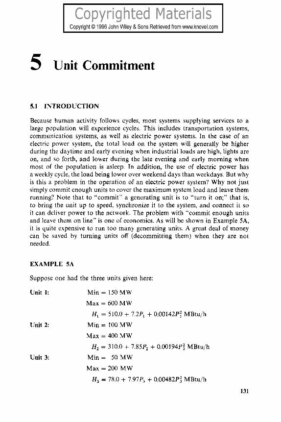
If we are to supply a load of 550 MW, what unit or combination of units should be used to supply this load most economically? To solve this problem, simply try all combinations of the three units. Some combinations will be infeasible if the sum of all maximum MW for the units committed is less than the load or if the sum of all minimum MW for the units committed is greater than the load. For each feasible combination, the units will be dispatched using the techniques of Chapter 3. The results are presented in Table 5.1.

Note that the least expensive way to supply the generation is not with all three units running, or even any combination involving two units. Rather, the optimum commitment is to only run unit 1, the most economic unit. By only running the most economic unit, the load can be supplied by that unit operating closer to its best efficiency. If another unit is committed, both unit 1 and the other unit will be loaded further from their best efficiency points such that the net cost is greater than unit 1 alone.

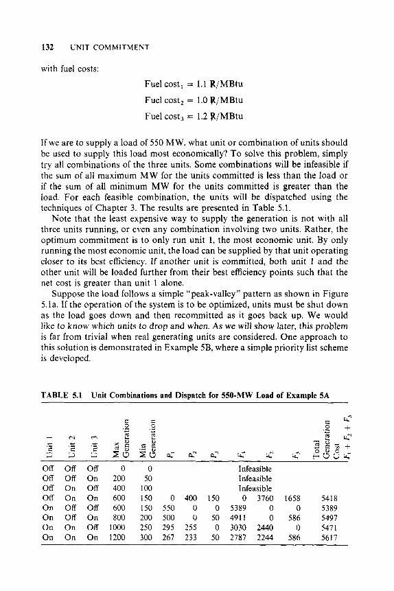
Suppose the load follows a simple “peak-valley’’ pattern as shown in Figure 5.la. If the operation of the system is to be optimized, units must be shut down as the load goes down and then recommitted as it goes back up. We would like to know which units to drop and when. As we will show later, this problem is far from trivial when real generating units are considered. One approach to this solution is demonstrated in Example 5B, where a simple priority list scheme is developed.

TABLE 5.1 Unit Combinations and Dispatch for 550-MW Load of Example 5A

off Off Off 0 0 Off Off On 200 50 Off On Off 400 100 Off On On 600 150 0 400 150 On Off Off 600 150 550 0 0 On Off On 800 200 500 0 50 On On Off 1000 250 295 255 0 On On On I200 300 267 233 50

Infeasible Infeasible Infeasible 0 3760 1658 5418

5389 0 0 5389 491 1 0 586 5497 3030 2440 0 5471 2787 2244 586 5617

INTRODUCTION 133

I

4 PM 4 AM 4 PM Time of day

FIG. 5.la Simple “peak-valley” load pattern.

4 PM 4 AM 4 PM Time of day

FIG, 5.lb Unit commitment schedule using shut-down rule.

EXAMPLE 5B

Suppose we wish to know which units to drop as a function of system load. Let the units and fuel costs be the same as in Example 5A, with the load varying from a peak of 1200 MW to a valley of 500 MW. To obtain a “shut-down rule,” simply use a brute-force technique wherein all combinations of units will be tried (as in Example 5A) for each load value taken in steps of 50 MW from 1200 to 500. The results of applying this brute-force technique are given in Table 5.2. Our shut-down rule is quite simple.

When load is above 1000 MW, run all three units; between 1000 MW and 600 MW, run units 1 and 2; below 600 MW, run only unit 1.

134 UNIT COMMITMENT

TABLE 5.2 “Shut-down Rule” Derivation for Example 5B Optimum Combination

Load Unit 1 Unit 2 Unit 3 ~

1200 1150 1100 1050 lo00 950 900 850 800 750 700 650 600 5 50 500

O n On O n On On On On On On On On On On O n O n

On O n On On On On On On On On On O n Off Off Off

O n O n On On Off Off Off Off Off Off Off Off Off Off Off

Figure 5.lb shows the unit commitment schedule derived from this shut-down rule as applied to the load curve of Figure 5.la.

So far, we have only obeyed one simple constraint: Enough units will be committed to supply the loud. If this were all that was involved in the unit commitment problem-that is, just meeting the load-we could stop here and state that the problem was “solved.” Unfortunately, other constraints and other phenomena must be taken into account in order to claim an optimum solution. These constraints will be discussed in the next section, followed by a description of some of the presently used methods of solution.

5.1.1 Constraints in Unit Commitment

Many constraints can be placed on the unit commitment problem. The list presented here is by no means exhaustive. Each individual power system, power pool, reliability council, and so forth, may impose different rules on the scheduling of units, depending on the generation makeup, load-curve characteristics, and such.

5.1.2 Spinning Reserve

Spinning reserve is the term used to describe the total amount of generation available from all units synchronized (i.e., spinning) on the system, minus the

INTRODUCTION 135

present load and losses being supplied. Spinning reserve must be carried so that the loss of one or more units does not cause too far a drop in system frequency (see Chapter 9). Quite simply, if one unit is lost, there must be ample reserve on the other units to make up for the loss in a specified time period.

Spinning reserve must be allocated to obey certain rules, usually set by regional reliability councils (in the United States) that specify how the reserve is to be allocated to various units. Typical rules specify that reserve must be a given percentage of forecasted peak demand, or that reserve must be capable of making up the loss of the most heavily loaded unit in a given period of time. Others calculate reserve requirements as a function of the probability of not having sufficient generation to meet the load.

Not only must the reserve be sufficient to make up for a generation-unit failure, but the reserves must be allocated among fast-responding units and slow-responding units. This allows the automatic generation control system (see Chapter 9) to restore frequency and interchange quickly in the event of a generating-unit outage.

Beyond spinning reserve, the unit commitment problem may involve various classes of “scheduled reserves” or “off-line” reserves. These include quick-start diesel or gas-turbine units as well as most hydro-units and pumped-storage hydro-units that can be brought on-line, synchronized, and brought up to full capacity quickly. As such, these units can be “counted” in the overall reserve assessment, as long as their time to come up to full capacity is taken into account.

Reserves, finally, must be spread around the power system to avoid transmission system limitations (often called “bottling” of reserves) and to allow various parts of the system to run as “islands,” should they become electrically disconnected.

EXAMPLE 5C

Suppose a power system consisted of two isolated regions: a western region and an eastern region. Five units, as shown in Figure 5.2, have been committed to supply 3090 MW. The two regions are separated by transmission tie lines that can together transfer a maximum of 550 MW in either direction. This is also shown in Figure 5.2. What can we say about the allocation of spinning reserve in this system?

The data for the system in Figure 5.2 are given in Table 5.3. With the exception of unit 4, the loss of any unit on this system can be covered by the spinning reserve on the remaining units. Unit 4 presents a problem, however. If unit 4 were to be lost and unit 5 were to be run to its maximum of 600 MW, the eastern region would still need 590 MW to cover the load in that region. The 590 MW would have to be transmitted over the tie lines from the western region, which can easily supply 590 MW from its reserves. However, the tie capacity of only 550 MW limits the transfer. Therefore, the loss of unit 4 cannot

136 UNIT COMMITMENT

550MW , t- maximum Units

1, 2, and 3

Western region I -I

Units 4 and 5

4 Eastern region

FIG. 5.2 Two-region system.

TABLE 5.3 Data for the System in Figure 5.2

Regional Unit Unit Genera- Regional Inter-

Capacity Output tion Spinning Load change Region Unit (MW) (MW) (MW) Reserve (MW) (MW)

Western 1 1000 900 100 2 800 420} 1740 380 1900 160 in 3 800 420 380

1190 160 out 160 '040} 1350 290 5 600 310

Eastern 4 1200

Total 1-5 4400 3090 3090 1310 3090

be covered even though the entire system has ample reserves. The only solution to this problem is to commit more units to operate in the eastern region.

5.1.3 Thermal Unit Constraints

Thermal units usually require a crew to operate them, especially when turned on and turned off. A thermal unit can undergo only gradual temperature changes, and this translates into a time period of some hours required to bring the unit on-line. As a result of such restrictions in the operation of a thermal plant, various constraints arise, such as:

0 Minimum up time: once the unit is running, it should not be turned off

0 Minimum down time: once the unit is decommitted, there is a minimum immediately.

time before it can be recommitted.

INTRODUCTION 137

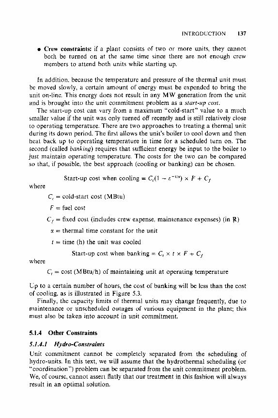
0 Crew constraints: if a plant consists of two or more units, they cannot both be turned on at the same time since there are not enough crew members to attend both units while starting up.

In addition, because the temperature and pressure of the thermal unit must be moved slowly, a certain amount of energy must be expended to bring the unit on-line. This energy does not result in any MW generation from the unit and is brought into the unit commitment problem as a start-up cost.

The start-up cost can vary from a maximum “cold-start” value to a much smaller value if the unit was only turned off recently and is still relatively close to operating temperature. There are two approaches to treating a thermal unit during its down period. The first allows the unit’s boiler to cool down and then heat back up to operating temperature in time for a scheduled turn on. The second (called banking) requires that sufficient energy be input to the boiler to just maintain operating temperature. The costs for the two can be compared so that, if possible, the best approach (cooling or banking) can be chosen.

Start-up cost when cooling = Cc(l - E - ’ ’ ‘ ) x F + C, where

C, = cold-start cost (MBtu)

F = fuel cost

C, = fixed cost (includes crew expense, maintenance expenses) (in p) SI = thermal time constant for the unit

t = time (h) the unit was cooled

Start-up cost when banking = C, x t x F + C,

C, = cost (MBtu/h) of maintaining unit at operating temperature

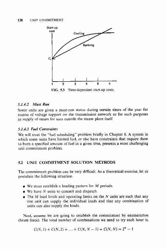
Up to a certain number of hours, the cost of banking will be less than the cost of cooling, as is illustrated in Figure 5.3.

Finally, the capacity limits of thermal units may change frequently, due to maintenance or unscheduled outages of various equipment in the plant; this must also be taken into account in unit commitment.

where

5.1.4 Other Constraints

5.1.4.1 Hydro-Constraints

Unit commitment cannot be completely separated from the scheduling of hydro-units. In this text, we will assume that the hydrothermal scheduling (or “coordination”) problem can be separated from the unit commitment problem. We, of course, cannot assert flatly that our treatment in this fashion will always result in an optimal solution.

138 UNIT COMMITMENT

1 2 3 4 5 h

FIG. 5.3 Time-dependent start-up costs.

5.1.4.2 Must Run Some units are given a must-run status during certain times of the year for reason of voltage support on the transmission network or for such purposes as supply of steam for uses outside the steam plant itself.

5.1.4.3 Fuel Constraints We will treat the “fuel scheduling” problem briefly in Chapter 6 . A system in which some units have limited fuel, or else have constraints that require them to burn a specified amount of fuel in a given time, presents a most challenging unit commitment problem.

5.2 UNIT COMMITMENT SOLUTION METHODS

The commitment problem can be very difficult. As a theoretical exercise, let us postulate the following situation.

0 We must establish a loading pattern for M periods. 0 We have N units to commit and dispatch. 0 The M load levels and operating limits on the N units are such that any

one unit can supply the individual loads and that any combination of units can also supply the loads.

Next, assume we are going to establish the commitment by enumeration (brute force). The total number of combinations we need to try each hour is,

C ( N , 1) + C ( N , 2 ) + . . . + C(N, N - 1) + C ( N , N ) = 2N - 1

UNIT COMMITMENT SOLUTION METHODS 139

where C ( N , j ) is the combination of N items taken j at a time. That is,

N ! C(N,J’) = [ ] ( N - j ) ! j !

j ! = 1 x 2 x 3 x . . . x j

For the total period of M intervals, the maximum number of possible combinations is (2N - l)M, which can become a horrid number to think about.

For example, take a 24-h period (e.g., 24 one-hour intervals) and consider systems with 5, 10, 20, and 40 units. The value of (zN - 1)24 becomes the following.

5 6.2 1035 10 1.73 1 0 7 2

20 3.12 10144

40 (Too big)

These very large numbers are the upper bounds for the number of enumera- tions required. Fortunately, the constraints on the units and the load-capacity relationships of typical utility systems are such that we do not approach these large numbers. Nevertheless, the real practical barrier in the optimized unit commitment problem is the high dimensionality of the possible solution space.

The most talked-about techniques for the solution of the unit commitment problem are:

0 Priority-list schemes, 0 Dynamic programming (DP), 0 Lagrange relation (LR).

5.2.1 Priority-List Methods

The simplest unit commitment solution method consists of creating a priority list of units. As we saw in Example 5B, a simple shut-down rule or priority-list scheme could be obtained after an exhaustive enumeration of all unit combinations at each load level. The priority list of Example 5B could be obtained in a much simpler manner by noting the full-load average production cost of each unit, where the full-load average production cost is simply the net heat rate at full load multiplied by the fuel cost.

140 UNIT COMMITMENT

EXAMPLE 5D

Construct a priority list for the units of Example SA. (Use the same fuel costs as in Example 5A.) First, the full-load average production cost will be calculated:

Unit Full Load

Average Production Cost (e /MWh)

1 9.79 2 9.48 3 11.188

A strict priority order for these units, based on the average production cost, would order them as follows:

Unit VliMWh Min MW Max MW

2 9.48 100 400 1 9.79 150 600 3 11.188 50 200

and the commitment scheme would (ignoring min up/down time, start-up costs, etc.) simply use only the following combinations.

Min MW from Corn bination Combination Combination

Max MW from

2 + 1 + 3 300 1200 2 + l 250 1000 2 100 400

Note that such a scheme would not completely parallel the shut-down sequence described in Example 5B, where unit 2 was shut down at 600 MW leaving unit 1. With the priority-list scheme, both units would be held on until load reached 400 MW, then unit 1 would be dropped.

Most priority-list schemes are built around a simple shut-down algorithm that might operate as follows.


0 At each hour when load is dropping, determine whether dropping the next unit on the priority list will leave sufficient generation to supply the load plus spinning-reserve requirements. If not, continue operating as is; if yes, go on to the next step.

0 Determine the number of hours, H , before the unit will be needed again. That is, assuming that the load is dropping and will then go back up some hours later.

0 If H is less than the minimum shut-down time for the unit, keep commitment as is and go to last step; if not, go to next step.

0 Calculate two costs. The first is the sum of the hourly production costs for the next H hours with the unit up. Then recalculate the same sum for the unit down and add in the start-up cost for either cooling the unit or banking it, whichever is less expensive. If there is sufficient savings from shutting down the unit, it should be shut down, otherwise keep it on.

0 Repeat this entire procedure for the next unit on the priority list. If it is also dropped, go to the next and so forth.

Various enhancements to the priority-list scheme can be made by grouping of units to ensure that various constraints are met. We will note later that dynamic-programming methods usually create the same type of priority list for use in the D P search.

5.2.2 Dynamic-Programming Solution

5.2.2.1 Introduction Dynamic programming has many advantages over the enumeration scheme, the chief advantage being a reduction in the dimensionality of the problem. Suppose we have found units in a system and any combination of them could serve the (single) load. There would be a maximum of 24 - 1 = 15 combinations to test. However, if a strict priority order is imposed, there are only four combinations to try:

Priority 1 unit Priority 1 unit + Priority 2 unit Priority 1 unit + Priority 2 unit + Priority 3 unit Priority 1 unit + Priority 2 unit + Priority 3 unit + Priority 4 unit

The imposition of a priority list arranged in order of the full-load average- cost rate would result in a theoretically correct dispatch and commitment only if:

142 UNIT COMMITMENT

1. No load costs are zero. 2. Unit input-output characteristics are linear between zero output and full

load. 3. There are no other restrictions. 4. Start-up costs are a fixed amount.

In the dynamic-programming approach that follows, we assume that:

1 . A state consists of an array of units with specified units operating and

2. The start-up cost of a unit is independent of the time it has been off-line

3. There are no costs for shutting down a unit. 4. There is a strict priority order, and in each interval a specified minimum

the rest off-line.

(i.e., it is a fixed amount).

amount of capacity must be operating.

A feasible state is one in which the committed units can supply the required load and that meets the minimum amount of capacity each period.

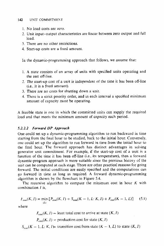
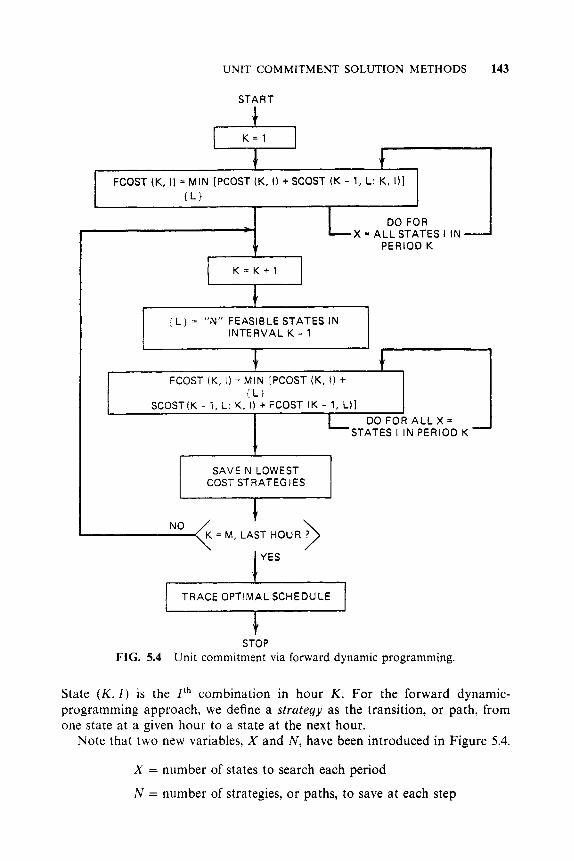
5.2.2.2 Forward DP Approach One could set up a dynamic-programming algorithm to run backward in time starting from the final hour to be studied, back to the initial hour. Conversely, one could set up the algorithm to run forward in time from the initial hour to the final hour. The forward approach has distinct advantages in solving generator unit commitment. For example, if the start-up cost of a unit is a function of the time it has been off-line (i.e., its temperature), then a forward dynamic-program approach is more suitable since the previous history of the unit can be computed at each stage. There are other practical reasons for going forward. The initial conditions are easily specified and the computations can go forward in time as long as required. A forward dynamic-programming algorithm is shown by the flowchart in Figure 5.4.

The recursive algorithm to compute the minimum cost in hour K with combination I is,

Fco,,(K, 1) = min CPco,,(K, I ) + S,,,,(K - 1, L: K , I) + F,,,,(K - 1, L)] (5.1) (LI

where

Fc,,,(K, I ) = least total cost to arrive at state ( K , I )

Pcost(K, I ) = production cost for state ( K , I )

S,,,,(K - 1, L: K , I )= transition cost from state ( K - 1, L) to state ( K , I )


I FCOST (K, I) = MIN (PCOST (K, I) + SCOST (K - 1, L: K, I ) ]

( L l

DO FOR -, X = ALL STATES I IN -

DO FOR ALL X =

\ t

I { K = K + l

I 1 { L } = "N" FEASIBLE STATES IN INTERVAL K - 1

TRACE OPTIMAL SCHEDULE

STOP FIG. 5.4 Unit commitment via forward dynamic programming.

State ( K , 1 ) is the Z t h combination in hour K . For the forward dynamic- programming approach, we define a strategy as the transition, or path, from one state at a given hour to a state at the next hour.

Note that two new variables, X and N , have been introduced in Figure 5.4.

X = number of states to search each period

N = number of strategies, or paths, to save at each step

144 UNIT C O M M I T M E N T

N X

0 0

0 0 0

interval Interval Interval K - 1 K K + 1

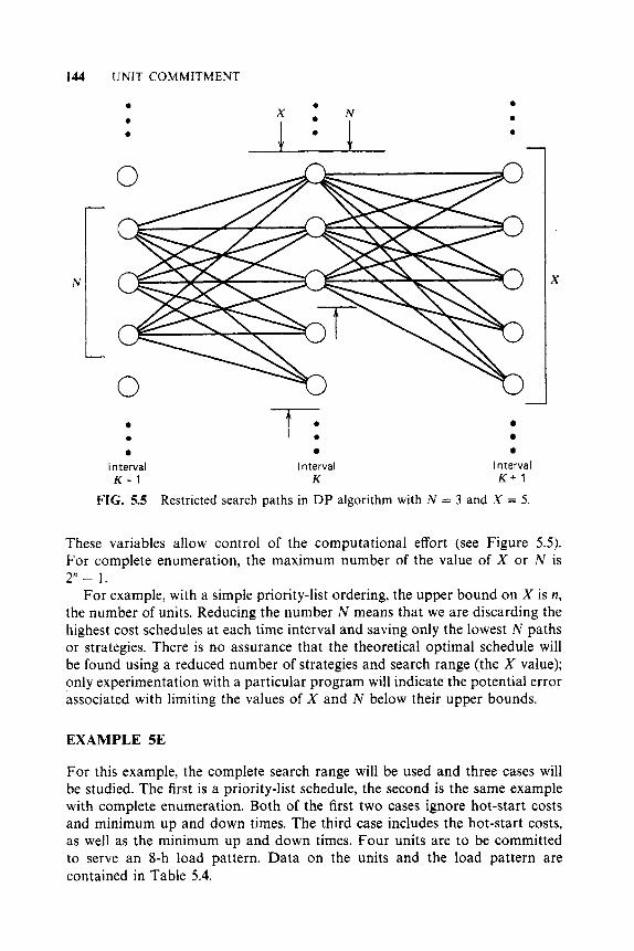
Restricted search paths in DP algorithm with N = 3 and X = 5.

0 t : 0

FIG. 5.5

These variables allow control of the computational effort (see Figure 5.5). For complete enumeration, the maximum number of the value of X or N is 2” - 1.

For example, with a simple priority-list ordering, the upper bound on X is n, the number of units. Reducing the number N means that we are discarding the highest cost schedules at each time interval and saving only the lowest N paths or strategies. There is no assurance that the theoretical optimal schedule will be found using a reduced number of strategies and search range (the X value); only experimentation with a particular program will indicate the potential error associated with limiting the values of X and N below their upper bounds.

EXAMPLE 5E

For this example, the complete search range will be used and three cases will be studied. The first is a priority-list schedule, the second is the same example with complete enumeration. Both of the first two cases ignore hot-start costs and minimum up and down times. The third case includes the hot-start costs, as well as the minimum up and down times. Four units are to be committed to serve an 8-h load pattern. Data on the units and the load pattern are contained in Table 5.4.


TABLE 5.4 Unit Characteristics, Load Pattern, and Initial Status for the Cases in Example 5E

Minimum Incremental No-Load Full-Load Times (h)

Max Min Heat Rate cost Ave. Cost Unit (MW) (MW) (Btu/kWh) (P/h) (F/mWh) Up Down 1 80 25 10440 213.00 23.54 4 2 2 2 50 60 9000 585.62 20.34 5 3 3 300 1 5 8730 684.74 19.74 5 4 4 60 20 11900 252.00 28.00 1 1

Initial Conditions Start-up Costs Hours Off-Line (-) Hot Cold Cold Start

Unit or On-Line (+) (bl) (PI (h) 1 -5 150 350 4 2 8 170 400 5 3 8 500 1 loo 5 4 -6 0 0.02 0

Load Pattern ~ ~~

Hour Load (MW)

1 450 2 530 3 600 4 540 5 400 6 280 7 290 8 500

In order to make the required computations more efficiently, a simplified model of the unit characteristics is used. In practical applications, two- or three-section stepped incremental curves might be used, as shown in Figure 5.6. For our example, only a single step between minimum and the maximum power points is used. The units in this example have linear F ( P ) functions:


I I

rl I I +

I I

MW Min Max output

( b )

FIG. 5.6 (a) Single-step incremental cost curve and (b) multiple-step incremental cost curve.

The F ( P ) function is:

F ( P ) = No-load cost + Inc cost x P

Note, however, that the unit must operate within its limits. Start-up cost$ for the first two cases are taken as the cold-start costs. The priority order for the four units in the example is: unit 3, unit 2, unit 1, unit 4. For the first two cases, the minimum up and down times are taken as 1 h for all units.

In all three cases we will refer to the capacity ordering of the units. This is shown in Table 5.5, where the unit combinations or states are ordered by maximum net capacity for each combination.

Case 1

In Case 1, the units are scheduled according to a strict priority order. That is, units are committed in order until the load is satisfied. The total cost for the interval is the sum of the eight dispatch costs plus the transitional costs for starting any units. In this first case, a maximum of 24 dispatches must be considered.


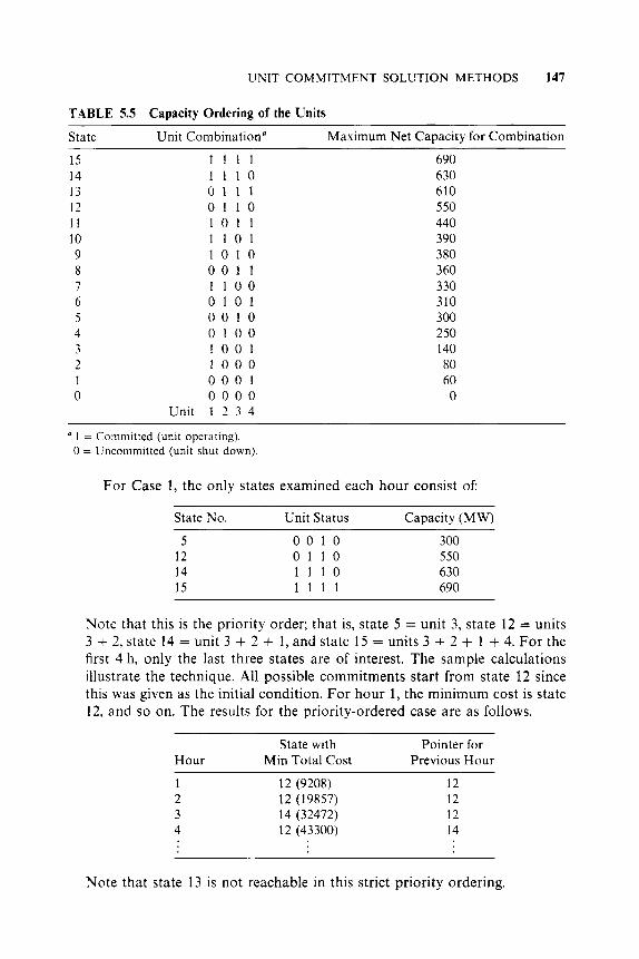
TABLE 5.5 Capacity Ordering of the Units

State Unit Combination" Maximum Net Capacity for Combination

15 14 13 12 1 1 10 9 8 7 6 5 4 3 2 1 0

1 1 1 1 1 1 1 0 0 1 1 1 0 1 1 0 1 0 1 1 1 1 0 1 1 0 1 0 0 0 1 1 I 1 0 0 0 1 0 1 0 0 1 0 0 1 0 0 1 0 0 1 1 0 0 0 0 0 0 1 0 0 0 0

Unit 1 2 3 4

690 630 610 550 440 390 380 360 330 310 300 250 140 80 60 0

' 1 = Committed (unit operating). 0 = Uncommitted (unit shut down).

For Case 1, the only states examined each hour consist of:

State No. Unit Status Capacity (MW)

5 0 0 1 0 300 12 0 1 1 0 550 14 1 1 1 0 630 15 1 1 1 1 690

Note that this is the priority order; that is, state 5 = unit 3, state 12 = units 3 + 2, state 14 = unit 3 + 2 + 1, and state 15 = units 3 + 2 + 1 + 4. For the first 4 h, only the last three states are of interest. The sample calculations illustrate the technique. All possible commitments start from state 12 since this was given as the initial condition. For hour 1, the minimum cost is state 12, and so on. The results for the priority-ordered case are as follows.

State with Pointer for Hour Min Total Cost Previous Hour 1 12 (9208) 12 2 12 (19857) 12 3 14 (32472) 12 4 12 (43300) 14

~~

Note that state 13 is not reachable in this strict priority ordering.

148 U N I T C O M M I T M E N T

Sample Calculations for Case 1

Allowable states are

{ } = (0010, 0110, 1110, 1111) = ( 5 , 12, 14, 15}

In hour O{L} = {12}, initial condition.

J = 1: 1st hour

K 15 - Fco,,( 1, 15) = PC,,,( 1,15) + Scos,(O, 12: 1, 15)

= 9861 + 350 = 10211

14

12

Fc,,,(l, 14) = 9493 + 350 = 9843

Fcost(l, 12) = 9208 + 0 = 9208

J = 2 2nd hour

are saved at each stage, so N = 2, and { L ) = { 12, 14}, Feasible states are (12, 14, 15) = ( K } , so X = 3. Suppose two strategies

and so on.

Case 2

In Case 2, complete enumeration is tried with a limit of (24 - 1) = 15 dispatches each of the eight hours, so that there is a theoretical maximum of 158 = 2.56. lo9 possibilities. Fortunately, most of these are not feasible because they do not supply sufficient capacity, and can be discarded with little analysis required.

Figure 5.7 illustrates the computational process for the first 4 h for Case 2. On-the figure itself, the circles denote states each hour. The numbers within the circles are the “pointers.” That is, they denote the state number in the previous hour that provides the path to that particular state in the current hour. For example, in hour 2, the minimum costs for states 12, 13, 14, and 15, all result from transitions from state 12 in hour 1. Costs shown on the connections are the start-up costs. At each state, the figures shown are the hourly cost/total cost.


State Unit number status - -

15

14

13

12

11 I

!

1111

1110

01 T 1

01 10

101 1

I I I I

/ ! I !

3;;; - N n w - .-

Total Capaaty

MW

690 -

630

610

550

440

I !

load 450 I 0 0 0 0 0---

I I I I

I I I I I I

FIG. 5.7 Example SE, Cases 1 and 2 (first 4 h).

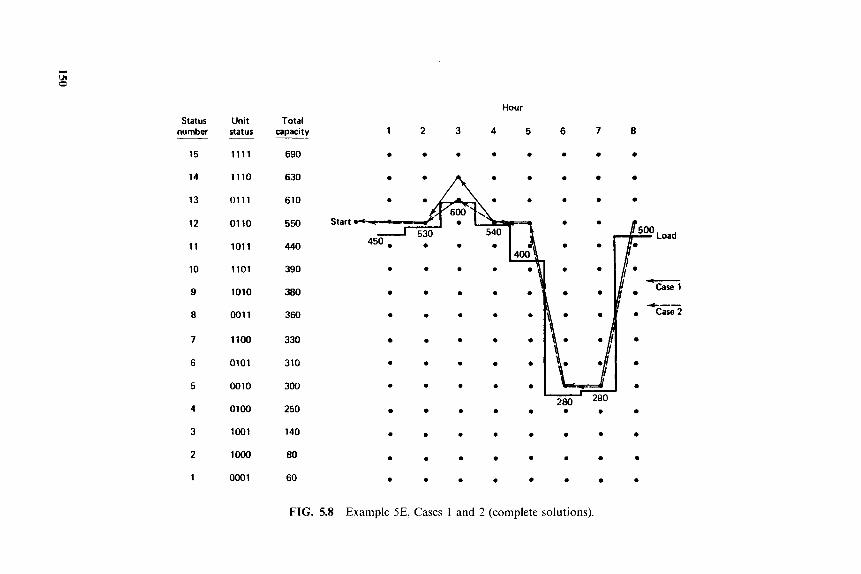
In Case 2, the true optimal commitment is found. That is, it is less expensive to turn on the less efficient peaking unit, number 4, for hour 3, than to start up the more efficient unit 1 for that period. By hour 3, the difference in total cost is p165, or pO.I04/MWh. This is not an insignificant amount when compared with the fuel cost per MWh for an average thermal unit with a net heat rate of 10,000 Btu/kWh and a fuel cost of p2.00 MBtu. A savings of p165 every 3 h is equivalent to p481,800/yr.

The total 8-h trajectories for Cases 1 and 2 are shown in Figure 5.8. The neglecting of start-up and shut-down restrictions in these two cases permits the shutting down of all but unit 3 in hours 6 and 7. The only difference in the two trajectories occurs in hour 3, as discussed in the previous paragraph.

Case 3

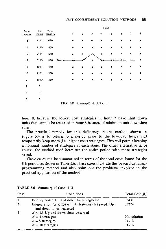
In case 3, the original unit data are used so that the minimum shut-down and operating times are observed. The forward dynamic-programming algorithm was repeated for the same 8-h period. Complete enumeration was used. That is, the upper bound on X shown in the flowchart was 15. Three different values for N , the number of strategies saved at each stage, were taken as 4, 8, and 10. The same trajectory was found for values of 8 and 10. This trajectory is shown in Figure 5.9. However, when only four strategies were saved, the procedure flounders (i.e., fails to find a feasible path) in

r-

.

w.

O.

N.

. .......

...... N

0.

.

....... ....... ....... ....... ...

...

... Y 0 - 2 ... s v hl

-u

... 3 - l)i

... s 0

150

UNIT COMMITMEMT SOLUTION METHODS 151

Hour State Unit Total

5 6 7 8

15 1111 690 0 0 . . b . 0

number status capacity 1 2 3 4 - --

14 1110 630 m . 0 * . 0

13 0111 610 0 0 . 0

12 0110 550 Start,

11 1011 440 m m b . * 0

10 1101 390 0 0 0 .

9 1010 380 0 0 b . * . 0

0 0

1 1

1 1

1 1

FIG. 5.9 Example 5E, Case 3.

hour 8, because the lowest cost strategies in hour 7 have shut down units that cannot be restarted in hour 8 because of minimum unit downtime rules.

The practical remedy for this deficiency in the method shown in Figure 5.4 is to return to a period prior to the low-load hours and temporarily keep more (i.e., higher cost) strategies. This will permit keeping a nominal number of strategies at each stage. The other alternative is, of course, the method used here: run the entire period with more strategies saved.

These cases can be summarized in terms of the total costs found for the 8-h period, as shown in Table 5.6. These cases illustrate the forward dynamic- programming method and also point out the problems involved in the practical application of the method.

TABLE 5.6 Summary of Cases 1-3

Case Conditions Total Cost (p) 1 Priority order. Up and down times neglected 73439 2 Enumeration ( X I 15) with 4 strategies ( N ) saved. Up 73274

and down times neglected 3 X I 15. Up and down times observed

N = 4 strategies B = 8 strategies N = 10 strategies

No solution 74110 74110

152 UNIT COMMITMENT

5.2.3 Lagrange Relaxation Solution

The dynamic-programming method of solution of the unit commitment problem has many disadvantages for large power systems with many generating units. This is because of the necessity of forcing the dynamic-programming solution to search over a small number of commitment states to reduce the number of combinations that must be tested in each time period.

In the Lagrange relaxation technique these disadvantages disappear (although other technical problems arise and must be addressed, as we shall see). This method is based on a dual optimization approach as introduced in Appendix 3A and further expanded in the appendix to this chapter. (The reader should be familiar with both of these appendices before proceeding further.)

We start by defining the variable U : as:

15': = 0 if unit i is off-line during period t

U : = 1 if unit i is on-line during period t

We shall now define several constraints and the objective function of the unit commitment problem:

1. Loading constraints: N

Pioad - 1 P:U: = 0 for t = 1 . . . T (5.2) i = l

2. Unit limits:

U:PT'" I P : I U:P$aX for i = 1 . . . N and t = 1 . . . T (5.3)

3. Unit minimum up- and down-time constraints. Note that other constraints can easily be formulated and added to the unit commitment problem. These include transmission security constraints (see Chapter 1 l), generator fuel limit constraints, and system air quality constraints in the form of limits on emissions from fossil-fired plants, spinning reserve constraints, etc.

4. The objective function is:

T N

C C [&(Pi) + Start up C O S ~ ~ , ~ ] U : = F(P: , U : ) (5.4) t = 1 i = l

We can then form the Lagrange function similar to the way we did in the economic dispatch problem:

N

t = 1 i = 1

The unit commitment problem requires that we minimize the Lagrange function


above, subject to the local unit constraints 2 and 3, which can be applied to each unit separately. Note:

1. The cost function, F(P:, Vi), together with constraints 2 and 3 are each separable over units. That is, what is done with one unit does not affect the cost of running another unit, as far as the cost function and the unit limits (constraint 2) and the unit up- and down-time (constraint 3) are concerned.

2. Constraints 1 are coupling constraints across the units so that what we do to one unit affects what will happen on other units if the coupling constraints are to be met.

The Lagrange relaxation procedure solves the unit commitment problem by “relaxing” or temporarily ignoring the coupling constraints and solving the problem as if they did not exist. This is done through the dual optimization procedure as explained in the appendix of this chapter. The dual procedure attempts to reach the constrained optimum by maximizing the Lagrangian with respect to the Lagrange multipliers, while minimizing with respect to the other variables in the problem; that is:

where q(L) = min Y ( P , U , 3.)

P : , a: (5.7)

This is done in two basic steps:

Step 1 Step 2

Find a value for each 3.‘ which moves q(%) toward a larger value. Assuming that the ir found in step 1 are now fixed, find the minimum of Y by adjusting the values of P’ and U‘.

The adjustment of the 1.’ values will be dealt with at a later time in this section; assume then that a value has been chosen for all the 3,‘ and that they are now to be treated as fixed numbers. We shall minimize the Lagrangian as follows.

First, we rewrite the Lagrangian as:

1 = 1 i = 1

T N

227 = 2 c [F,(P:) + Start up costi,,]Uf + Pioad - 2 P ; U ; ) (5 .8) f = l i = l

This is now rewritten as:

154 UNIT COMMITMENT

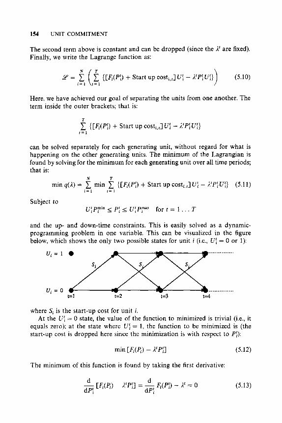
The second term above is constant and can be dropped (since the I' are fixed). Finally, we write the Lagrange function as:

{ [ & ( P : ) + Start up costi,,] U : - I ~ . ' P : u ~ }

Here, we have achieved our goal of separating the units from one another. The term inside the outer brackets; that is:

T

can be solved separately for each generating unit, without regard for what is happening on the other generating units. The minimum of the Lagrangian is found by solving for the minimum for each generating unit over all time periods; that is:

N T min q ( A ) = 1 min 1 { [&(Pi ) + Start up costi,,]U: - I'P:U:} (5.11)

i = 1 t = 1

Subject to U:Py'" I Pi I U : P y for t = 1 . . . T

and the up- and down-time constraints. This is easily solved as a dynamic- programming problem in one variable. This can be visualized in the figure below, which shows the only two possible states for unit i (i.e., U : = 0 or 1):

-.-__-.-.-.-.. u i = l 0

ui = 0 t=l Lxx t=2 t=3 t=4 ......-.-.-...

where Si is the start-up cost for unit i. At the U : = 0 state, the value of the function to minimized is trivial (i.e., it

equals zero); at the state where U : = 1, the function to be minimized is (the start-up cost is dropped here since the minimization is with respect to P:):

min [&(PJ - A'P:] (5.12)

The minimum of this function is found by taking the first derivative:

(5.13)


The solution to this equation is

(5.14)

There are three cases to be concerned with depending on the relation of Ppp' and the unit limits:

1. If Ppp' 5 Pyi". then:

min [&(pi) - A'p:] = &(PT'") - A'pyin (5.15a)

2. If Pyin I PpP' I Pya", then:

min [&(pi) - A'P:] = &(PpP') - A f P p p t (5.15b)

3. If Ppp' 2 Pyx, then:

min [4(4) - n'Pi] = F,(Py") - A',? (5.15~)

The solution of the two-state dynamic program for each unit proceeds in the normal manner as was done for the forward dynamic-programming solution of the unit commitment problem itself. Note that since we seek to minimize [&(P;.) - i 'Pi] at each stage and that when U : = 0 this value goes to zero, then the only way to get a value lower is to have

[&(pi) - 2 P : ] < 0

The dynamic program should take into account all the start-up costs, Si, for each unit, as well as the minimum up and down time for the generator. Since we are solving for each generator independently, however, we have avoided the dimensionality problems that affect the dynamic-programming solution.

5.2.3.1 Adjusting rZ So far, we have shown how to schedule generating units with fixed values of 1' for each time period. As shown in the appendix to this chapter, the adjustment of A' must be done carefully so as to maximize q(A). Most references to work on the Lagrange relaxation procedure use a combination of gradient search and various heuristics to achieve a rapid solution. Note that unlike in the appendix, the ;1 here is a vector of values, each of which must be adjusted. Much research in recent years has been aimed at ways to speed the search for the correct values of 2 for each hour. In Example 5D, we shall use the same technique of adjusting A for each hour that is used in the appendix. For the unit commitment problem solved in Example 5D, however, the A adjustment factors are different:

(5.16)


where

(5.17) d d l

tl = 0.01 when - 4(%) is positive

and

(5.18) d dA

LY = 0.002 when - 4(A) is negative

Each E.‘ is treated separately. The reader should consult the references listed at the end of this chapter for more efficient methods of adjusting the 3, values. The overall Lagrange relaxation unit commitment algorithm is shown in Figure 5.10.

Reference 15 introduces the use of what this text called the “relative duality gap” or ( J * - 4*)/4*. The relative duality gap is used in Example 5D as a measure of the closeness to the solution. Reference 15 points out several useful things about dual optimization applied to the unit commitment problem.

1. For large, real-sized, power-system unit commitment calculations, the duality gap does become quite small as the dual optimization proceeds, and its size can be used as a stopping criterion. The larger the problem (larger number of generating units), the smaller the gap.

2. The convergence is unstable at the end, meaning that some units are being switched in and out, and the process never comes to a definite end.

3. There is no guarantee that when the dual solution is stopped, it will be at a feasible solution.

All of the above are demonstrated in Example 5D. The duality gap is large at the beginning and becomes progressively smaller as the iterations progress. The solution reaches a commitment schedule when at least enough generation is committed so that an economic dispatch can be run, and further iterations only result in switching marginal units on and off. Finally, the loading constraints are not met by the dual solution when the iterations are stopped.

Many of the Lagrange relaxation unit commitment programs use a few iterations of a dynamic-programming algorithm to get a good starting point, then run the dual optimization iterations, and finally, at the end, they use heuristic logic or restricted dynamic programming to get to a final solution. The result is a solution that is not limited to search windows, such as had to be done in strict application of dynamic programming.

EXAMPLE 5D

In this example, a three-generator, four-hour unit commitment problem will be solved. The data for this problem are as follows. Given the three generating


.

Pick starting h' for t=l ... T k = O

feasibility

update h' for all t

3

Build dynamic program having two states, and T stages and solve for:

Pf and Ui for all t = 1...T ,

No + last unit done

Yes

Solve for the dual value 9*(h')

Using the U' calculate the primal value J: that is, solve an economic dispatch for each hour using the units that have been committed for that hour

units below:

Fl(Pl) = 500 + 10Pl + 0.002P: and

F2(P2) = 300 + 8P2 + 0.0025P: and

F3(P3) = 100 + 6P3 + O.OOSP,Z and

100 < Pl < 600

100 < P2 < 400

50 < P3 < 200


Load:

1 170 2 520 3 1100 4 330

No start-up costs, no minimum up- or down-time constraints. This example is solved using the Lagrange relaxation technique. Shown

below are the results of several iterations, starting from an initial condition where all the i.' values are set to zero. An economic dispatch is run for each hour, provided there is sufficient generation committed that hour. If there is not enough generation committed, the total cost for that hour is set arbitrarily to 10,000. Once each hour has enough generation committed, the primal value J * simply represents the total generation cost summed over all hours as calculated by the economic dispatch.

The dynamic program for each unit with a ;C' = 0 for each hour will always result in all generating units off-line.

Iteration 1 ~ -

N

Hour 2 u1 u2 u3 P, P2 P3 Pioad - 1 P ! U : Peldc P'Z"' P5dc , = I

1 0 0 0 0 0 0 0 170 0 0 0 2 0 0 0 0 0 0 0 520 0 0 0 3 0 0 0 0 0 0 0 1100 0 0 0 4 0 0 0 0 0 0 0 330 0 0 0

J* - q* q ( A ) = 0.0, J* = 40,000, and ~ = undefined

4*

In the next iteration, the I' values have been increased. To illustrate the use of dynamic programming to schedule each generator, we will detail the DP steps for unit 3:

x = 1.7 5.2 11.0 3.3 F ( P ) - x P = 327.5 152.5 -700.0 247,s

3 3 p? = pmin p3 3 = p3 m a P': = p p p ; = p p

u 3 = 1 u3 = 0 t= cj/\ 1 t=2 t=3 t-Q cost= min -700


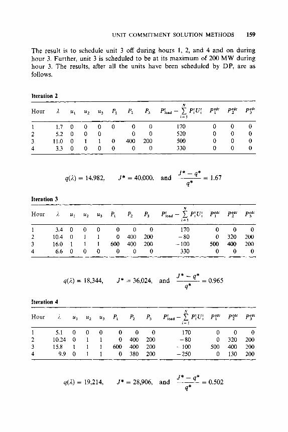
The result is to schedule unit 3 off during hours 1, 2, and 4 and on during hour 3. Further, unit 3 is scheduled to be at its maximum of 200 MW during hour 3. The results, after all the units have been scheduled by DP, are as follows.

Iteration 2 ~~

N

Hour 1 U 1 U 2 113 p2 P3 Pfoad - 1 Piui P:dc P.;"' P';"' i = 1

1 1.7 0 0 0 0 0 0 170 0 0 0 2 5.2 0 0 0 0 0 520 0 0 0 3 11.0 0 1 1 0 400 200 500 0 0 0 4 3.3 0 0 0 0 0 0 330 0 0 0

J* - q* q(A) = 14,982, J * = 40,000, and ___ - - 1.67

4*

Iteration 3

1 3.4 0 0 0 0 0 0 170 0 0 0 2 10.4 0 1 1 0 400 200 - 80 0 320 200 3 16.0 1 1 1 600 400 200 - 100 500 400 200 4 6.6 0 0 0 0 0 0 330 0 0 0

J * - q* q(A) = 18,344, J * = 36,024, and ~ = 0.965

4*

Iteration 4

Hour 2 u1 t i2 u3 Pl P2 P3 Pfoad - 1 P!U: P:dc P;dc P;dc N

i = 1

1 5.1 0 0 0 0 0 0 170 0 0 0 2 10.24 0 1 1 0 400 200 - 80 0 320 200 3 15.8 1 1 1 600 400 200 - 100 500 400 200 4 9.9 0 1 1 0 380 200 - 250 0 130 200

J * - q* q(L) = 19,214, J * = 28,906, and ____ - - 0.502

4*


Iteration 5

Hour i u1 u2 uj PI P2 P3 Piaad - P:Ui P;dc P;dc Pedc 3 N

i = 1

1 6.8 0 0 0 0 0 0 170 0 0 0 2 10.08 0 1 1 0 400 200 - 80 0 320 200 3 15.6 1 1 1 600 400 200 - 100 500 400 200 4 9.4 0 0 1 0 0 200 130 0 0 0

q(2) = 19.532, J * = 36,024, and J * - q* ~- - 0.844

4*

Iteration 6 N

Hour i u 1 u2 u3 P, P2 P3 Pioad - 1 P : U : P:dc P g C P5dc i = 1

1 8.5 0 0 1 0 0 200 - 30 0 0 170 2 9.92 0 1 1 0 384 200 - 64 0 320 200 3 15.4 1 1 1 600 400 200 -100 500 400 200 4 10.7 0 1 1 0 400 200 - 270 0 130 200

J * - q* q(2) = 19,442, J* = 20,170, and ___ - - 0.037

4*

The commitment schedule does not change significantly with further iterations, although i t is not by any means stable. Further iterations do reduce the duality gap somewhat, but these iterations are unstable in that unit 2 is on the borderline between being committed and not being committed, and is switched in and out with no final convergence. After 10 iterations, q(A) = 19,485, J * = 20,017, and ( J * - q*)/q* = 0.027. This latter value will not go to zero, nor will the solution settle down to a final value; therefore, the algorithm must stop when ( J * - q*)/q* is sufficiently small (e.g., less than 0.05 in this case).

APPENDIX Dual Optimization on a Nonconvex Problem

We introduced the concept of dual optimization in Appendix 3A and pointed out that when the function to be optimized is convex, and the variables are continuous, then the maximization of the dual function gives the identical result as minimizing the primal function. Dual optimization is also used in solving the unit commitment problem. However, in the unit commitment problem there are variables that must be restricted to two values: 1 or 0. These 1-0 variables

DUAL OPTIMIZATION O N A NONCONVEX PROBLEM 161

cause a great deal of trouble and are the reason for the difficulty in solving the unit commitment problem.

The application of the dual optimization technique to the unit commitment problem has been given the name “Lagrange relaxation” and the formulation of the unit commitment problem using this method is shown in the text in Section 5.2.3. In this appendix, we illustrate this technique with a simple geometric problem. The problem is structured with 1-0 variables which makes it clearly nonconvex. Its form is generally similar to the form of the unit commitment problems, but that is incidental for now.

The sample problem to be solved is given below. It illustrates the ability of the dual optimization technique to solve the unit commitment problem. Given:

J(x,, x2, ul, u 2 ) = (0 .25~: + 15)u1 + (0.255~: + 15)u2 (5A.1)

subject to:

and

0 5 x2 I 10

(5A.2)

(5A.3)

(5A.4)

where x l and x2 are continuous real numbers, and:

ul = 1 or 0

u2 = 1 or 0

Note that in this problem we have two functions, one in x1 and the other in x2. The functions were chosen to demonstrate certain phenomena in a dual optimization. Note that the functions are numerically close and only differ by a small, constant amount. Each of these functions is multiplied by a 1-0 variable and combined into the overall objective function. There is also a constraint that combines the x1 and x2 variables again with the 1-0 variables. There are four possible solutions.

1. If u1 and u2 are both zero, the problem cannot have a solution since the equality constraint cannot be satisfied.

2. If u1 = I and u2 = 0, we have the trivial solution that x1 = 5 and x2 does not enter into the problem anymore. The objective function is 21.25.

3. If u1 = 0 and u2 = 1, then we have the trivial result that x2 = 5 and x1 does not enter into the problem. The objective function is 21.375.

4. If u1 = 1 and u2 = 1, we have a simple Lagrange function of:

9 ( x 1 , x2, E.) = (0 .25~: + 15) + (0.255~: + 15) + 4 5 - x1 - x2) (5A.5)

The resulting optimum is at x1 = 2.5248, x2 = 2.4752, and ;1 = 1.2642, with an

162 UNIT COMMITMENT

objective function value of 33.1559. Therefore, we know the optimum value for this problem; namely, u1 = 1, u2 = 0, and x1 = 5.

What we have done, of course, is to enumerate all possible combinations of the 1-0 variables and then optimize over the continuous variables. When there are more than a few 1-0 variables, this cannot be done because of the large number of possible combinations. However, there is a systematic way to solve this problem using the dual formulation.

The Lagrange relaxation method solves problems such as the one above, as follows. Define the Lagrange function as:

9 ( x l , x2, ul, u2, A) = (0.25~: + 15)U1 + ( 0 . 2 5 5 ~ : + 1 5 ) U 2

+ A(5 - X l U l - x2u2) (5A.6)

As shown in Appendix 3A, we define q(A) as:

(5A.7)

where xl, x2, ul, u2 obey the limits and the 1-0 conditions as before. The dual problem is then to find

q*(A) = max q(A) 120

(5A.8)

This is different from the dual optimization approach used in the Appendix 3A because of the presence of the 1-0 variables. Because of the presence of the 1-0 variables we cannot eliminate variables; therefore, we keep all the variables in the problem and proceed in alternating steps as shown in the Appendix 3A.

Step 1 Pick a value for 1.k and consider it fixed. Now the Lagrangian function can be minimized. This is much simpler than the situation we had before since we are trying to minimize

(0 .25~: + 15)u, + ( 0 . 2 5 5 ~ : + 15)u2 + Ak(5 - xlul - x2u2)

where the value of Ak is fixed. We can then rearrange the equation above as:

( 0 . 2 5 ~ : + 15 - x lAk)u l + ( 0 . 2 5 5 ~ : + 15 - x ~ A ~ ) u ~ + Ak5

The last term above is fixed and we can ignore it. The other terms are now given in such a way that the minimization of this function is relatively easy. Note that the minimization is now over two terms, each being multiplied by a 1-0 variable. Since these two terms are summed in the Lagrangian, we can minimize the entire function by

DUAL OPTIMIZATION ON A NONCONVEX PROBLEM 163

minimizing each term separately. Since each term is the product of a function in x and A (which is fixed), and these are all multiplied by the 1-0 variable u, then the minimum will be zero (that is with u = 0) or it will be negative, with u = 1 and the value of x set so that the term inside the parentheses is negative. Looking at the first term, the optimum value of x1 is found by (ignore u1 for a moment):

d - (0.25~: + 15 - x~A') = 0 dx 1

(5A.9)

If the value of x1 which satisfies the above falls outside the limits of 0 and 10 for xl , we force x1 to the limit violated. If the term in the first brackets

(0.25~: + 15 - x1Ak)

is positive, then we can minimize the Lagrangian by merely setting u1 = 0; otherwise u1 = 1.

Looking at the second term, the optimum value of x2 is found by (again, ignore uz):

d - (0.255~: + 15 - xzAk) = 0 dx2

(5A.10)

and if the value of x2 which satisfies the above value falls outside the 0 to 10 limits on x2, we set it to the violated limit. Similarly, the term in the second brackets

(0.255~: + 15 - ~22')

is evaluated. If it is positive, then we minimize the Lagrangian by making u2 = 0; otherwise u2 = 1. We have now found the minimum value of 2' with a specified fixed value of I.".

Step 2 Assume that the variables xl, x2, ul, u2 found in step 1 are fixed and find a value for A that maximizes the dual function. In this case, we cannot solve for the maximum since 4(A) is unbounded with respect to A. Instead, we form the gradient of q(A) with respect to A and we adjust A so as to move in the direction of increasing q(A). That is, given

which for our problem is

(5A.11)

(5A.12)

164 UNIT COMMITMENT

we adjust A according to

(5A.13)

where u is a multiplier chosen to move A only a short distance. (This is simply a gradient search method as was introduced in Chapter 3). Note also, that if both u1 and u2 are zero, the gradient will be 5, indicating a positive value telling us to increase A. Eventually, increasing 1 will result in a negative value for

(0.25~: + 15 - ~ ~ 2 . k ) or for

(0.255~: + 15 - x2Ak)

or for both, and this will cause u1 or u2, or both, to be set to 1. Once the value of i. is increased, we go back to step 1 and find the new values for xl, x2, u l , u2 again.

The real difficulty here is in not increasing 1 by too much. In the example presented above, the following scheme was imposed on the adjustment of I.:

dq d /.

0 If is positive, then use c( = 0.2.

dq ’ 0 If - is negative, then use u = 0.005.

d 1.

This lets 1. approach the solution slowly, and if it overshoots, it backs up very slowly. This is a common technique to make a gradient “behave.”

We must also note that, given the few variables we have, and given the fact that two of them are 1-0 variables, the value of 2, will not converge to the value needed to minimize the Lagrangian. In fact, it is seldom possible to find a that will make the problem feasible with respect to the equality constraint. However, when we have found the values for u1 and u2 at any iteration, we can then calculate the minimum of J(xl, x2, ul, u 2 ) by solving for the minimum of

C(0.25~: + 15)u1 + (0.255~: + 15)u2 + 4 5 - xlul - x 2 u 2 ) ]

using the techniques in Appendix 3A (since the u1 and u2 variables are now known).

The solution to this minimum will be at x1 = sr;, x2 = x2 and A = 1. For the case where u1 and u2 are both zero, we shall arbitrarily set this value to a large value (here we set it to 50). We shall call this minimum value

-

TABLE 5.7 Dual Optimization on a Sample Problem

Iteration 1. u1 u2 X I x2 w i J*

0 1 .o 2.0 3.0 4.0 3.9458 3.8926 3.8787

0 0 0 0 0 0 0 0 1 1 1 1 1 0 1 0

0 2.0 4.0 6.0 8.0 7.8916 7.7853 7.7574

0 1.9608 3.9216 5.8824 7.843 1 7.7368 7.6326 7.6053

0 5.0

10.0 15.0 18.3137 18.8958 19.3105 19.3491

5.0 5.0 5.0 5.0

- 10.8431 - 10.6284 -2.7853 - 2.7574

1.2624 1.2624 2.5 2.5

-

2.5248 2.5248 5.0 5.0

2.4752 2.4752

50.0 50.0 50.0 50.0 33.1559 33.1559 21.25 21.25

- 9.0 4.0 2.33 0.8104 0.7546 0.1004 0.0982

166 UNIT COMMITMENT

J * ( q , K, u l , u2) and we shall observe that it starts out with a large value, and decreases, while the dual value q*(A) starts out with a value of zero, and increases. Since there are 1-0 variables in this problem, the primal values and the dual values never become equal. The value J * - q* is called the duality gap and we shall call the value

J * - q*

4* the relative duality gap.

The presence of the 1-0 variables causes the algorithm to oscillate around a solution with one or more of the 1-0 variables jumping from 1 to 0 to 1, etc. In such cases, the user of the Lagrange relaxation algorithm must stop the algorithm, based on the value of the relative duality gap.

The iterations starting from A = 0 are shown in Table 5.7. The table shows eight iterations and illustrates the slow approach of I toward the threshold when both of the 1-0 variables flip from 0 to 1. Also note that o became negative and the value of I must now be decreased. Eventually, the optimal solution is reached and the relative duality gap becomes small. However, as is typical with the dual optimization on a problem with 1-0 variables, the solution is not stable and if iterated further it exhibits further changes in the 1-0 variables as i. is adjusted. Both the q* and J * values and the relative duality gap are shown in Table 5.7.

PROBLEMS

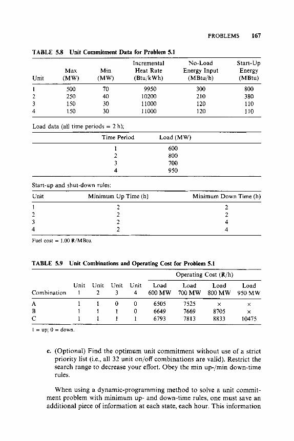
5.1 Given the unit data in Tables 5.8 and 5.9, use forward dynamic- programming to find the optimum unit commitment schedules covering the 8-h period. Table 5.9 gives all the combinations you need, as well as the operating cost for each at the loads in the load data. A " x " indicates that a combination cannot supply the load. The starting conditions are: at the beginning of the first period units 1 and 2 are up, units 3 and 4 are down and have been down for 8 h.

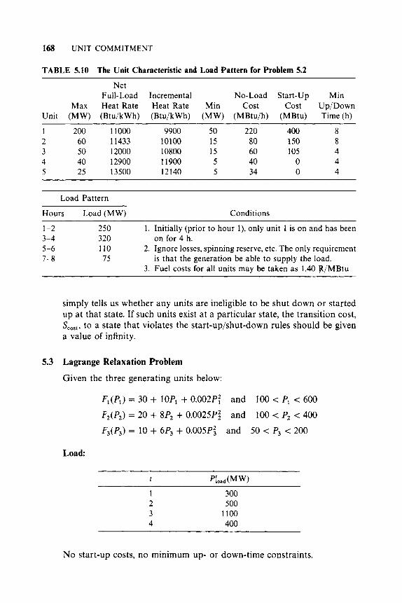
5.2 Table 5.10 presents the unit characteristics and load pattern for a five-unit, four-time-period problem. Each time period is 2 h long. The input-output characteristics are approximated by a straight line from min to max generation, so that the incremental heat rate is constant. Unit no-load and start-up costs are given in terms of heat energy requirements. a. Develop the priority list for these units and solve for the optimum unit

commitment. Use a strict priority list with a search range of three ( X = 3) and save no more than three strategies ( N = 3). Ignore min up-/min down-times for units.

b. Solve the same commitment problem using the strict priority list with X = 3 and N = 3 as in part a, but obey the min up/min down time rules.

PROBLEMS 167

TABLE 5.8 Unit Commitment Data for Problem 5.1

Incremental No-Load Start-up Max Min Heat Rate Energy Input Energy

Unit (MW) (MW) (Bt u/k W h) (M Btu/h) (MBtu)

1 500 70 9950 300 800 2 250 40 10200 210 380 3 150 30 1 lo00 120 110 4 150 30 1 lo00 120 110

Load data (all time periods = 2 h);

Time Period Load (MW)

600 800 700 950

Start-up and shut-down rules:

Unit Minimum Up Time (h) Minimum Down Time (h)

1 2 2 2 2 2 3 2 4 4 2 4

Fuel cost = 1.00 P/MBtu.

TABLE 5.9 Unit Combinations and Operating Cost for Problem 5.1

Operating Cost (P/h)

Unit Unit Unit Unit Load Load Load Load Combination 1 2 3 4 600MW 700MW 800MW 950MW

A 1 1 0 0 6505 7525 X X

B 1 1 1 0 6649 7669 8705 X

C 1 1 1 1 6793 7813 8833 10475

1 = up; 0 = down.

c. (Optional) Find the optimum unit commitment without use of a strict priority list (i.e., all 32 unit on/off combinations are valid). Restrict the search range to decrease your effort. Obey the min up-/min down-time rules.

When using a dynamic-programming method to solve a unit commitment problem with minimum up- and down-time rules, one must save an additional piece of information at each state, each hour. This information


TABLE 5.10 The Unit Characteristic and Load Pattern for Problem 5.2 ~ ~~ ~~ ~~ ~~~

Net Full-Load Incremental No-Load Start-up Min

Max Heat Rate Heat Rate Min Cost Cost Up/Down Unit (MW) (Btu/kWh) (Btu/kWh) (MW) (MBtu/h) (MBtu) Time (h)

1 200 11000 9900 50 220 400 8 2 60 11433 10100 15 80 150 8 3 50 12000 10800 15 60 105 4 4 40 12900 11900 5 40 0 4 5 25 13500 12140 5 34 0 4

Load Pattern

Hours Load (MW) Conditions ~ ~ ~~ ~ ~ ~

1-2 3-4 320 on for 4 h. 5-6 7-8

250

110 75

1. Initially (prior to hour I), only unit 1 is on and has been

2. Ignore losses, spinning reserve, etc. The only requirement

3. Fuel costs for all units may be taken as 1.40 ft/MBtu is that the generation be able to supply the load.

simply tells us whether any units are ineligible to be shut down or started up at that state. If such units exist at a particular state, the transition cost, S,,,,, to a state that violates the start-up/shut-down rules should be given a value of infinity.

5.3 Lagrange Relaxation Problem

Given the three generating units below:

Fl(Pl) = 30 + 10Pl + 0.002P: and

F,(Pz) = 20 + 8P2 + 0.0025P: and

F3(P3) = 10 + 6P3 + 0.005Pi and 50 < P3 < 200

100 < Pl < 600

100 < Pz < 400

Load:

~

t PlO*d(MW) 1 300 2 500 3 1100 4 400

No start-up costs, no minimum up- or down-time constraints.

FURTHER READING 169

a. Solve for the unit commitment by convent ional dynamic programming. b. Set up and carry o u t four iterations of the Lagrange relaxation method.

c. Resolve with the added condi t ion tha t the third generator has a Let the initial values of A‘ be zero for t = 1 . , .4.

minimum up time of 2 h.

FURTHER READING

Some good introductory references to the unit commitment problem are found in references 1-3. A survey of the state-of-the-art (as of 1975) of unit commitment solutions is found in reference 4. References 5 and 6 provide a good look at two commercial unit commitment programs in present use.

References 7-1 1 deal with unit commitment as an integer-programming problem. Much of the pioneering work in this area was done by Garver (reference 7), who also sounded a note of pessimism in a discussion of reference 8, written together with Happ in 1968. Further research (references 9-1 1) has refined the unit commitment solution by integer programming but has never really overcome the Garver-Happ limitations presented in the 1968 discussion, thus leaving dynamic programming and Lagrange relaxation as the only viable solution techniques to large-scale unit commitment problems.

The reader should see references 12 and 13 for a discussion of valve-point loading and for a thorough development of economic dispatch via dynamic programming.

Reference 14 provides the reader with a good overview of unit commitment scheduling. References 15, 16, and 17 are recommended for an understanding of the Lagrange relaxation method, while references 18-21 cover some of the special problems encountered in unit commitment scheduling.

1. Baldwin, C . J., Dale, K. M., Dittrich, R. F., “A Study of Economic Shutdown of Generating Units in Daily Dispatch,” AIEE Transactions on Power Apparatus and Systems, Vol. PAS-78, December 1959, pp. 1272-1284.

2. Burns, R. M., Gibson, C. A., “Optimization of Priority Lists for a Unit Commitment Program,” IEEE Power Engineering Society Summer Meeting, Paper A-75-453-1, 1975.

3. Davidson, P. M., Kohbrman, F. J., Master, G. L., Schafer, G. R., Evans, J. R., Lovewell, K. M., Payne, T. B., “Unit Commitment Start-Stop Scheduling in the Pennsylvania-New Jersey-Maryland Interconnection,” 1967 PICA Conference Proceedings, IEEE, 1967, pp. 127-132.

4. Gruhl, J., Schweppe, F., Ruane, M., “Unit Commitment Scheduling of Electric Power Systems,” Systems Engineering for Power: Status and Prospects, Henniker, NH, US. Government Printing Office, Washington, DC, 1975.

5. Pang, C. K., Chen, H. C., “Optimal Short-Term Thermal Unit Commitment,’’ IEEE Transactions on Power Apparatus and Systems, Vol. PAS-95, July/August 1976,

6. Happ, H. H., Johnson, P. C., Wright, W. J., “Large Scale Hydro-Thermal Unit Commitment-Method and Results,” IEEE Transactions on Power Apparatus and Systems, Vol. PAS-90, May/June 1971, pp. 1373-1384.

7. Garver, L. L., “Power Generation Scheduling by Integer Programming-

pp. 1336-1346.


Development of Theory,” AIEE Transactions on Power Apparatus and Systems, Vol. PAS-82, February 1963, pp. 730-735.

8. Muckstadt, J. A,, Wilson, R. C., “An Application of Mixed-Integer Programming Duality to Scheduling Thermal Generating Systems,” IEEE Transactions on Power Apparatus and Systems, Vol. PAS-87, December 1968, pp. 1968-1978.

9. Ohuchi, A,, Kaji, I., “ A Branch-and-Bound Algorithm for Start-up and Shut-down Problems of Thermal Generating Units,” Electrical Engineering in Japan, Vol. 95,

10. Dillon, T. S., Egan, G. T., “Application of Combinational Methods to the Problems of Maintenance Scheduling and Unit Commitment in Large Power Systems,” Proceedings of IFAC Symposium on Large Scale Systems Theory and Applications, Udine, Italy, 1976.

11. Dillon, T. S., Edwin, K. W., Kochs, H. D., Taud, R. J., “Integer Programming Approach to the Problem of Optimal Unit Commitment with Probabilistic Reserve Determination,” IEEE Transactions on Power Apparatus and Systems, Vol. 97, November/December 1978, pp. 2154-2166.

12. Happ, H. H., Ille, W. B., Reisinger, R. M., “Economic System Operation Considering Valve Throttling Losses, I-Method of Computing Valve-Loop Heat Rates on Multivalve Turbines,” IEEE Transactions on Power Apparatus and Systems, Vol. PAS-82, February 1963, pp. 609-615.

13. Ringlee, R. J., Williams, D. D., “Economic Dispatch Operation Considering Valve Throttling Losses, 11-Distribution of System Loads by the Method of Dynamic Programming,” IEEE Transactions on Power Apparatus and Systems, Vol. PAS-82, February 1963, pp. 615-622.

14. Cohen, A. I., Sherkat, V. R., “Optimization-Based Methods for Operations Scheduling, Proceedings IEEE, December 1987, pp. 1574-1591.

15. Bertsekas, D., Lauer, G. S., Sandell, N. R., Posbergh, T. A., “Optimal Short-Term Scheduling of Large-Scale Power Systems,” IEEE Transactions on Automatic Control, Vol. AC-28, No. 1, January 1983, pp. 1-11.

16. Merlin, A,, Sandrin, P., “A New Method for Unit Commitment at Electricite de France,” IEEE Transactions on Power Apparatus and Systems, Vol. PAS-102, May

17. Zhuang, F., Galiana, F. D., “Towards a More Rigorous and Practical Unit Commitment by Lagrangian Relaxation,” IEEE Transactions on Power Systems, Vol. 3, No. 2, May 1988, pp. 763-773.

18. Lee, F. N., Chen, Q., Breipohl, A,, “Unit Commitment Risk with Sequential Rescheduling,” IEEE Transactions on Power Systems, Vol. 6 , No. 3, August 1991,

19. Vemuri, S., Lemonidis, L., “Fuel Constrained Unit Commitment,” IEEE Transactions on Power Systems, Vol. 7, No. 1, February 1992, pp. 410-415.

20. Wang, C., Shahidepour, S. M., “Optimal Generation Scheduling with Ramping Costs,” 1993 IEEE Power Industry Computer Applications Conference, pp. 11-17.

21. Shaw, J. J., “A Direct Method for Security-Constrained Unit Commitment,” IEEE Transactions Paper 94 SM 591-8 PWRS, presented at the IEEE Power Engineering Society Summer Meeting, San Francisco, CA, July 1994.

NO. 5, 1975, pp. 54-61.

1983, pp. 1218-1225.

pp. 1017-1023.

3 unit commitmentcee.nit.ac.ir/file_part/master_doc/201422213549125916406660.pdf · 3 unit...

Documents