3. tropical cyclone motion - · 3. tropical cyclone motion 3.1 introduction ... (rappaport et al....

Chapter Three

Todd B. Kimberlain and Micheal J. Breman National Hurricane Center

NOAA/NWS/NCEP, Miami, Fl

3. Tropical Cyclone Motion

3.1 Introduction

While the prediction of tropical cyclone (TC) track remains a challenging problem, new tools to observe TCs have emerged in recent years to facilitate locating the TC center and estimating TC motion. The advent of new technology has coincided with remarkable progress in numerical weather prediction, which has helped to reduce typical TC track errors by half in the Atlantic basin at all lead times since 1990 (Rappaport et al. 2009). Similar improvement has been seen in the western North Pacific by the Japan Meteorological Agency and by the Joint Typhoon Warning Center. In fact, there has been dramatic improvement in all of the basins. This success is partially due to a tremendous increase in satellite data, which are particularly valuable in data-sparse regions such as the Tropics. The increase in observations and advances in data assimilation techniques have greatly improved the quality of initial condition analyses for regional and global dynamical models. The development of ensemble and consensus methods has also contributed to improvements in track forecasting. As a result of these advances, the performance of the regional and global dynamical models has far surpassed that of statistical and simple dynamical models.

This chapter describes contemporary approaches to analyzing TC position and forecasting TC track. The first section focuses on position analysis and the various observational platforms used in this task. A discussion of numerical model guidance applications and TC forecasting techniques follows in the second section, with particular emphasis on "ensemble" and "consensus" forecasting. The chapter concludes with a description of verification methods and their uses in an operational setting.

3.2 Position analysis

Construction of a best track

Operational best track

Locating the center of the TC is the first step in forecasting TC track, as it establishes the current motion of the cyclone. In an operational environment observations arrive from a wide array of platforms at different times. These observations contain errors, vary in spatial and

temporal coverage, and can be unrepresentative and contradictory. This makes the determination of the actual TC position and motion difficult. An accurate current motion estimate is important for diagnosing the interaction of the TC with the surrounding environment, evaluating the quality of the current forecast, and initializing some computer models. A center "fix" can be obtained by using any or all of the observational platforms described in the sections that follow. As a forecaster examines the fixes, determining the current position depends on the confidence in the observations and the forecaster’s judgment. For example, when the current position uncertainty is high (i.e., in the case of a poorly defined system or a system at night), a heavy reliance should be given to the previous positions established with greater confidence (i.e., during the daytime or when the center was better defined). Position estimates made with high confidence may also be helpful in revising the best track during the previous 24-hour period. After determining a preliminary position, the TC motion can be computed. The time period over which the current motion is calculated depends on the steadiness of the motion and the confidence in the accuracy of the center fix, with the goal of minimizing unrepresentative short-term motions such as trochoidal motion or other wobbles (Lawrence and Mayfield 1977). The track should be smoothed over this time period, and the re-analysis can be extended further in time if new data become available. A typical smoothing period for estimating the initial motion might be 18 hours, somewhat longer when uncertainty with regard to initial position is high (e.g., a poorly-defined IR fix) and somewhat less when the uncertainty is low (e.g., a good radar fix). Then, the bearing and speed of the TC are computed, and the new motion estimate is compared to that from the previous forecast cycle to ensure realistic values. Striking a balance between the high and low confidence scenarios described above is key to the process of maintaining an operational best track. When late satellite or synoptic data arrive, that data should be assessed, and if necessary, appropriate adjustments should be made to the working best track in order to improve the TC motion vector. Construction of a final best track A post-analysis review of operational track positions with data from a wide variety of sources should be conducted to optimally re-construct the best track of a TC. This type of analysis is generally not possible in real-time, since the "working best track" is developed under tight time constraints, when some data may not be available. The final product should satisfy the basic components of an accepted "best track" definition such as the one currently in place at the NHC: "A subjectively-smoothed representation of a TC's location and intensity over its lifetime. The best track contains the cyclone's latitude, longitude, maximum sustained surface wind, and minimum sea-level pressure at six-hourly intervals. Best track positions and intensities, which are based on a post-storm assessment of all available data, may differ from values contained in storm advisories. They also generally will not reflect the erratic motion implied by connecting individual center fixes."

A major consideration is the degree of detail to furnish when preparing the "best track." A fundamental part of NHC's "best track" definition is the six-hourly representative estimates of the cyclone's center location. Plotted raw fix data often reveal a series of irregular movements, which do not generally persist for more than a few hours (refer to the short-term motion section below). Short-term track wobbles are not representative of the overall TC motion, and a subjectively-smoothed "best track" that does not focus on these short period, transient motions is ideal. Some forecasters have interpreted this to mean that, if a TC is, in fact, located at a given position at 0600 UTC, the "best track" need not lie exactly at that location in post-analysis. From a sampling perspective, the re-positioning that results from the smoothing process is part of a filtering procedure that could be administered to avoid aliasing small-scale noise. For a time series with data points ΔT apart, the smallest wavelength which can be depicted accurately is about 4 x ΔT. Since the typical advisory analysis times are six hours apart, the smallest periods which can be adequately represented are on the order of 24 hours. Thus the analyst might try to avoid analyzing oscillations with a period less than 24 hours. The final best track estimate often differs a little from the real time advisory estimate because the former is meant to represent a particular time, while the latter is meant to be valid at a particular time. Satellite fixes The most common method of fixing a TC's location is through the use of geostationary satellite imagery. These satellites provide high temporal resolution visible and infrared (IR) imagery and are the primary tool for TC center fixing. Geostationary images can also be animated and modified with color enhancements that correspond to various brightness temperatures to help determine the location and motion of a TC center. In many cases, animating visible satellite imagery to examine low cloud motions is a reliable way to identify a TC center. However, if available, ocean vector wind data and 37 GHz microwave data can help refine the surface center position. At night it is often difficult to distinguish between low and high clouds in IR imagery, complicating the center fixing of weaker TCs. Nighttime "visible" imagery (Ellrod 1995) was developed to supplement conventional IR imagery for TC center fixing (Jiann-Gwo Jiing, personal communication). This imagery is created by merging the shortwave IR (3.9 micron) and longwave IR (11 micron) windows. The radiative properties of the shortwave window allow for the identification of low cloud features, while the longwave channel is more sensitive to the tops of deep convective clouds. Therefore, the merged product is useful for locating the center of sheared or poorly-organized TCs. However, its utility is limited if the low cloud pattern is obscured by cirrus. If available, 37 GHz microwave imagery can reveal the low-level center of sheared systems, even though the center is obscured by overlying cirrus.

Rules for locating the TC center with satellite imagery are contained in the Enhanced Infrared (EIR) version of the Dvorak (1984) technique. Figure 3.1 illustrates the typical cloud pattern evolution of TCs and how using pattern recognition can help the analyst determine the cloud system center (CSC). In addition to using the pictographs in Figure 3.1, several other methods such as drawing lines to visualize the curvature of bands and looping images at different speeds can also be used (Dvorak (1984, 1995). In the Dvorak technique, an accurate intensity analysis often requires an accurate center position. In fact, the Dvorak technique "assumes" that you "know" where the center is located. Using satellite imagery to identify the CSC does have limitations. For example, it is possible to mistake a mid-level center for the low-level center in weak or sheared systems. Also, mid- or high-level clouds may obscure the low-level center. The presence of multiple centers, especially within a broad monsoon disturbance, can also be a complicating factor. In this situation, the analyst should estimate a centroid location of the overall circulation and not focus on a single center. While conventional satellite imagery is vital to operational TC forecasting, aircraft reconnaissance data, if available, are nearly always favored over these satellite observations since aircraft fixes are in situ and are generally more accurate than satellite-based fixes. A National Hurricane Center (NHC) study showed that about a quarter of all satellite position estimates were in error by at least 20 nm, while aircraft reconnaissance position estimates had smaller errors when compared to final best track data. (Of course, aircraft data, when available, are somewhat more heavily weighted in the production of the best track.)

Figure 3.1. Typical cloud pattern evolution of an idealized TC, using the EIR Dvorak technique. The basic curved band (top row), CDO (middle row), or "shear" pattern

types (bottom row) with a standard developmental curve from left to right can be used to determine the CSC. Reproduced from Dvorak (1995).

Proper application of the Dvorak technique requires considerable training and practice. The original visual Dvorak technique has different application rules than the EIR technique. Intensity aspects of the technique are discussed in Chapter 4. Microwave satellite data The availability of microwave data for TC center fixing from low-earth orbiting satellites has increased in recent years. Passive radiometers sense emitted microwave radiation over a wide range of wavelengths, enabling them to see through clouds and discern structures difficult to observe using visible and infrared satellite imagery. Instrumentation As of 2010, a total of 13 low Earth orbiting (LEO) satellites were operational (Table 3.1) .

Table 3.1. Current suite of microwave polar orbiting instruments and the associated satellite.

Satellite Instrument Operati

ng Since Scan Strategy/ Type

Frequency (GHz)

No. of Channels

Resolution (km)

Swath Width (km)

NASA/DoD

Coriolis Windsat 2003-

conical, imager

6.8-371 22 11-55 1025

NASA/JAXA

TRMM TRMM (TMI) 1997-

conical, imager

10.65-85.5

9 5-50 780

Metop-A%

AMSU-A AMSU-B ASCAT

2006-

cross-track,

sounder scatterom

eter

23.8-89 85-

183.31 5.25

15 5

48 16

50(25)

1650 1650 2520

F-15 F-18

SSM/T2 SSM/I

1987- 2009-

cross-track,

sounder 92-183 5

*309 (85-213)#

1400

DMSP(F-16, F-17,

F-18) SSMIS 2004-

conical, imager & sounder

19-183 24 12-55 1700

Aqua AMSR-E 2002- conical, imager

6.9-89 14 5-50 1600

NOAA-15 NOAA-16 NOAA-18

AMSU 1998- 2000- 2005-

cross-track,

sounder 50-183 20

**50 (16)@ **150 (50)#

2200

1 WindSat channels at 10.7, 18.7, and 37 GHz are fully polarimetric @ at nadir # at limb $ pulse, fixed-point radar % METOP-B to be launched in 2012

A description of selected instruments is provided below:

• The Tropical Rainfall Measuring Mission (TRMM) flies in a near-equatorial orbit,measuring rainfall and other rainfall-related parameters using two different sensors.The passive TRMM Microwave Imager (TMI) detects rainfall by measuring the intensity ofbackscattered radiation at five frequencies between 10.7 and 85 GHz. As a consequenceof its lower orbital altitude, the satellite has smaller footprint sizes and higher resolution(6 km). The TMI is frequently used for TC observation because its mid-Earth orbit isconfined to the region between 35°N and 35°S.

• The Advanced Microwave Sounding Unit-B (AMSU-B) is a passive instrument on theNOAA series of polar-orbiting satellites. The AMSU instrument looks cross-track andtherefore its scan angle varies with distance from nadir.

• METOP-A is the first in a series of three polar-orbiting satellites flown by the EuropeanSpace Agency (ESA) carrying a high-resolution microwave imager similar to the AMSU-Bfound on the NOAA satellites.

• The Special Sensor Microwave Imager (SSM/I) is a microwave instrument onboardDefense Meteorological Satellite Program (DMSP) satellites.

• The SSMIS instrument is a follow-on and replacement for to the SSM/I. SSMIS is apassive, conically-scanning radiometer that has more spectral channels and a widerswath width than the SSM/I (1700 km compared to 1400 km).

• WindSat is one of two payloads aboard the U.S. Navy's Coriolis satellite launched in2003. It can measure wind speed and direction, although not reliably in the heavy rainenvironment of a TC's inner core. The multi-frequency polarimetric radiometer passivelymeasures emitted microwave radiation at five frequencies from 6.8 to 37 GHz. WindSatis a conical scanner with resolution about three times higher than the SSM/I.

• The Advancing Microwave Sounding Radiometer — Eos (AMSR-E) is a passive conically-scanning instrument flying on the NASA Aqua research satellite. It senses microwaveradiation at 12 different channels at six frequencies from 6.9 to 89 GHz.

The analyst can obtain a myriad of real-time and archived microwave imagery from the U.S. Navy's NRL or FNMOC TC web sites located at: http://www.nrlmry.navy.mil/tc_pages/tc_home.html.

Interpretation of microwave imagery

Data obtained at 85 to 91 GHz are primarily used to observe deep convective clouds, especially in the TC core. Within this region of the electromagnetic spectrum, cloud water droplets near the freezing level deplete upwelling microwave radiation. Since non-precipitating cirrus has

little effect on radiation at this wavelength, the remaining upwelled radiation is released to space, where satellites can observe it. The effects of scattering and absorption reduce the net microwave radiation aloft, making satellite brightness temperatures appear cold. An example of deep convective and cirrus clouds obscuring the center of developing eastern North Pacific Tropical Storm Georgette at 0411 UTC 27 August 2004 is shown in Figure 3.2. While the center is not apparent in the geostationary IR imagery (Fig. 3.2a,b), 85-GHz imagery from the SSM/I (Fig. 3.2c,d) clearly shows the exposed low-level center of the developing TC at the edge of the convective canopy.

Figure 3.2. (a and b) IR satellite imagery of Tropical Storm Georgette from 0245 UTC 27 August 2004, with no enhancement in (a) and the standard BD Dvorak curve in

(b). (c) SSM/I 85 GHz H pass from 0411 UTC over Georgette and (d) the composite image for the pass, illustrating the exposed low-level center located near 16.8N

109.1W.Data at lower frequencies (e.g., 37 GHz) are used to identify low cloud features. Emission and absorption of microwave radiation by hydrometeors near and

below the freezing level is minimal at this frequency, making observed brightness temperatures in areas of low clouds and precipitation appear warm.

Comparing data from 85-91 GHz and 37 GHz can help determine if the TC is experiencing vertical wind shear. Imagery at 85-91 GHz reveals features at middle- to upper-levels and can show the location of a mid-level center while imagery from 37 GHz can reveal low cloud features indicative of the low-level center position. Therefore, center fixes from these two channels may not be in agreement if the TC is sheared. The 37-GHz imager is better suited for

center fixes in weaker or sheared TCs, even though it is of lower resolution than the higher frequency channels on most satellites. Microwave radiation emitted from the Earth's surface and elsewhere in the atmosphere is initially unpolarized but its interaction with different atmospheric or Earth constituents can cause it to become partially polarized. This makes it possible to determine certain characteristics of the environment through which it is passing. For example, land and water differences become apparent when comparing horizontally polarized emissions at low microwave frequencies. The contrast between land, water, low clouds, or the ocean is more distinct when comparing composite microwave images of both horizontal and vertical polarizations against those from high and low frequency channels and can help to distinguish important features (as discussed next). Analysts should examine multiple channels/frequencies, polarizations, and composite images to determine the TC center location. Combining and cross-referencing center fixes obtained from multiple images can increase confidence in the TC position estimate. A brief, step-by-step procedure providing center fixes from an analysis of microwave images follows. A good starting point is to evaluate high and low frequency single polarization images. The 85-91 GHz images are easy to interpret because the cloud liquid water in low clouds (warm rain processes) at outer radii appears warm (darker blue in Fig. 3.3), while significantly colder brightness temperatures (yellows and red) depict radiometrically cold convective tops at a much higher level surrounding the eye. Next, lower frequency polarized images (e.g., Figs. 3.4-3.5) should be evaluated. Condensate in low clouds and rainbands appear warm relative to the radiometrically cold ocean surface at lower frequencies (Fig. 3.4). The warmest brightness temperatures are coincident with the greatest concentration of low-level cloud liquid water in the inner core. The center of incipient systems can sometimes be difficult to locate since increasing low-level convergence of cloud liquid water near the vortex can mask the center. Finally, the analyst should evaluate both high and low frequency color composite images, which use the Polarization Correction Temperature (PCT) solution to discriminate intense convection from both single polarized images. On the PCT image, one should focus on the blue-green colors, which primarily denote low-level clouds. In stronger storms, the TC center can be located by looking for a dark spot on the low frequency composite image, which should be the rain-free dry region. Figure 3.5 shows an example of a 37-GHz PCT image, where blue-green streamers indicate low cloud bands and reds and pinks indicate well-developed convective clouds. A dark green spot, representing an area that is the same temperature as the ocean surface, indicates the cloud-free eye. Analysis of multiple images (preferably within six hours of the analysis time) can increase the chances of correctly identifying the TC center. These sequential multiple images can be animated to improve center location of poorly organized systems (Edson, personal communication).

Figure 3.3. TRMM 85-GHz H-pol image over Hurricane Ike at 1905 UTC 3 September 2008. Brightness temperature (K) is indicated by the scale at the bottom of the

figure. Image courtesy of the U.S. Naval Research Laboratory.

Figure 3.4. As in Fig. 3.3, except TRMM 37-GHz V-pol image. Image courtesy of the U.S. Naval Research Laboratory.

Figure 3.5. As in Fig. 3.3, except TRMM 37-GHz Polarization Correction Temperature (PCT) image. Image courtesy of the U.S. Naval Research Laboratory.

Scanners onboard the various low earth-orbiting satellites are either cross-track or conical. Conical-scanning instruments look forward at a fixed angle with a rotating antenna, and footprints of equal size provide the same resolution across the entire swath (Fig. 3.6a). Cross-track instruments scan at varying angles as the instrument points away from nadir. As a result, these imagers have degraded resolution near the edge of the scan, where the footprint size is larger (Fig. 3.6b).

Figure 3.6. Illustration of (a) a conical scanner, which has a fixed viewing angle and a constant-sized footprint size across the swath, and (b) a cross-track scanner, which

scans at varying angles with higher resolution in the middle of the swath and lower resolution on the edges (courtesy of UCAR/COMET).

The difference between the two scanning techniques is apparent over western Pacific Super Typhoon Podul (Figs. 3.7-3.9). The AMSU-B 89-GHz image at 0246 UTC 25 October 2001 captures Podul at the edge of the swath, where the limitation of larger footprint size and a coarser resolution leads to an enlargement of the pixel size and a distortion of the image (Fig. 3.7). This distortion can severely hamper TC center fix estimates. The higher resolution 2228 UTC 24 October 2001 SSM/I image (Fig. 3.8) from a few hours earlier allows for a more precise TC center fix, demonstrating the superior quality of the conical scanner. Figure 3.9, an SSM/I image of Podul from 1036 UTC 25 October 2001, illustrates the high resolution of the SSM/I pass, even at the edge of the swath.

Figure 3.7. AMSU-B 89-GHz image of Super Typhoon Podul at 0246 UTC 25 October 2001, illustrating the poor resolution of the cross-track scanner at the edge of the

swath. Colors correspond to brightness temperatures (K) in the legend. Figure 3.8. SSM/I 85-GHz H-pol image of Super Typhoon Podul from 2228 UTC 24 October 2001, illustrating the superb resolution of the conical scanner across the

entire swath. Colors correspond to brightness temperatures (K) in the legend. Figure 3.9. SSM/I 85-GHz image of Super Typhoon Podul from 1036 UTC 25 October 2001, illustrating the high resolution of conical scanner at limb. Colors correspond

to brightness temperatures (K) in the legend.

Cautionary considerations

Microwave estimates of TC location should be used with some caution since the slanted viewing geometry of microwave polar-orbiting satellites displaces features slightly askew of their actual location (i.e., parallax error). Figure 3.10 illustrates the typical parallax error in the 85-GHz channel, where scattering of microwave radiation by ice particles is dominant and in the 37-GHz channel which mainly senses microwave radiation emitted from cloud water droplets in low clouds. Paired with the schematic drawings (Fig. 3.10a,c) are two nearly simultaneous microwave images over Typhoon Jelawat on 8 August 2000, which reveal the discrepancy in TC position between the two frequencies. Figure 3.10b shows Jelawat in 37 GHz imagery, with the red circle indicating the general location where the analyst might place the center. The 85-GHz imagery (Fig. 3.10d) reveals a much broader eyewall surrounding the center, with the yellow circle corresponding to a possible center fix. While parallax error is present in both images, the 15- to 20-km error in the 85-GHz channel is much larger than the 5-km error in the 37-GHz image. Smaller (greater) parallax error is typically observed in the 37-GHz (85-GHz) imagery because the particles sensed at this frequency are emitted from a lower (higher) altitude, reducing (increasing) the distortion caused by the viewing geometry.

Figure 3.10. Illustration of typical parallax error associated with two microwave channels. (a) shows an exaggerated cross-section of the parallax error from the 37-GHz

channel, while (c) shows the parallax error associated with the 85-91-GHz channels. (b) and (d) show parallax error observed in microwave imagery, with (b) showing

minor parallax error at 37-GHz and (d) showing more substantial parallax error at 85-GHz. Figure courtesy of UCAR/COMET. Microwave imagery presents a "snapshot" of the TC at a point and time. Since microwave imagery has relatively low temporal resolution, it may be difficult to determine if a feature in a single image is the true TC center. In Figure 3.11a, the forecaster may focus on the curved

convective clouds in the 89-GHz channel to fix the center of Tropical Storm Kevin. Comparing the microwave fix to the corresponding color composite image (Fig. 3.11b) could help confirm its accuracy. In some cases, however, errors may still occur, especially for weak TCs or pre-TC disturbances. For example, the actual center of Tropical Storm Kevin was located almost a degree farther south at this time (not shown).

Figure 3.11. (a) AMSR-E 89 GH-z image of Tropical Storm Kevin at 2157 UTC 30 August 2009. (b) AMSR-E Color Composite image of Tropical Storm Kevin at the same

time.Image navigation can also be problematic.If possible, a forecaster should inspect geographic features within the image to ensure that they are properly

located.However, it is not possible to identify image navigation errors for TCs over the open ocean because there is no land in the image. Data latency, the time between a satellite overpass and the successful transmission of its data to a ground receiving station for processing can result in a significant delay in the arrival of data for operational analysis. Figure 3.12 indicates the fraction of data available as a function of data latency. On average, nearly 80% of all data are available within five hours of overpass, but there are occasions when data arrive even later. The next generation of U.S. low earth orbiting satellites is expected to greatly reduce data latency with additional ground receiving sites and with 95% of all data likely available within 30 minutes of overpass (see NPOESS COMET module).

Figure 3.12. Plot of the fraction of microwave polar-orbiting data available to users in real time as a function of time. The x-axis or delay time is in hours, while the y-

axis or data fraction available to users is in %. Figure courtesy of UCAR/COMET. Scatterometry Scatterometers estimate near-surface wind speed and direction over the ocean surface by measuring the backscatter variations from small-scale roughness elements (capillary waves) on the ocean surface. The European Space Agency's Advanced Scatterometer (ASCAT) onboard the METOP satellite series will be described here. Although the NASA SeaWinds instrument onboard the QuikSCAT failed in late 2009, it will be discussed briefly as well, since there is a possibility that data from scatterometers similar to QuikSCAT will become available for TC analysis in the coming years. ASCAT is an operational scatterometer currently flying on the METOP satellite series (three missions are planned through 2020). ASCAT has two 550-km wide swaths and a 720-km nadir gap. Due to this swath configuration, ASCAT only provides about 60% of the coverage that was provided by QuikSCAT (Fig. 3.13), and the nadir gap results in few passes that sample the entire circulation of a TC. ASCAT wind retrievals are available at 50- and 25-km resolution and are noticeably smooth, as they were designed primarily for assimilation into numerical models. ASCAT exhibits a notable low wind bias at wind speeds above 30 kt compared to QuikSCAT and other observations (Cobb et al. 2008). Since ASCAT is a C-band scatterometer, its retrievals are less sensitive to rain than those from QuikSCAT were, which results in improved retrieval quality, particularly in weaker TCs.

Figure 3.13. Image showing typical, daily coverage of ASCAT (top) and QuikSCAT (bottom). Note the wider QuikSCAT swaths compared to ASCAT, with large gaps in

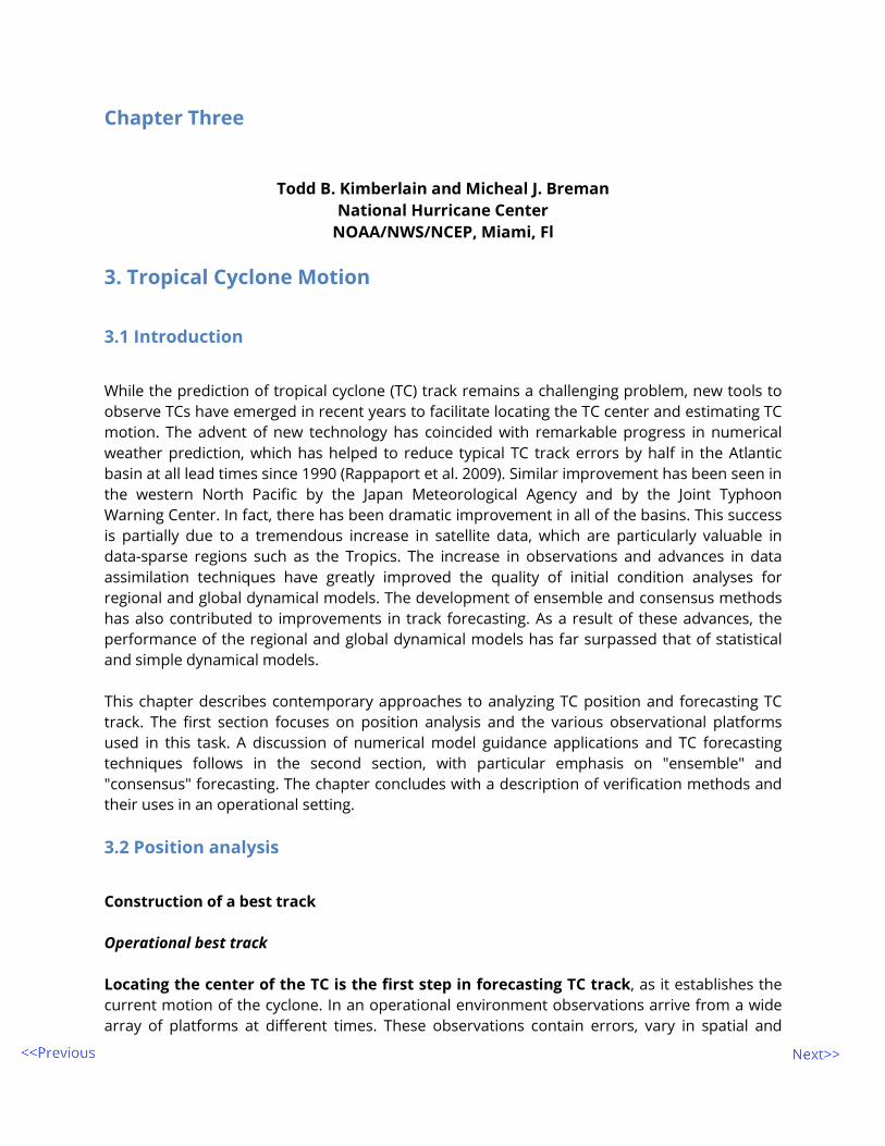
coverage from both sensors over the Tropics. Aerial reconnaissance data Aerial weather reconnaissance provides the best source of data to determine the center location of TCs. Even though aerial reconnaissance data have been used in TC forecasting since 1944 in the Atlantic, it is not used in most other global basins due to its prohibitive cost. In the Atlantic and sometimes in the Eastern and Central North Pacific basins, specially modified and equipped aircraft of the U.S. Air Force Reserve (AFRES) and the National Oceanic and Atmospheric Administration's Aircraft Operations Center (NOAA/AOC) are used to investigate TCs. A typical mission consists of the plane flying at 10,000 ft (700 hPa) for hurricanes and 5,000 ft (850 hPa) for tropical storms. For pre-TC disturbances (i.e., "invest" missions), the typical flight altitude is 1,500 ft (457 m). The plane flies a figure four or "alpha" pattern through the system (Fig. 3.14). Missions can last from 10 to 12 hours, with two to six center fixes possible. Aircraft observations from within the TC are generally restricted to locations along and near the flight path.

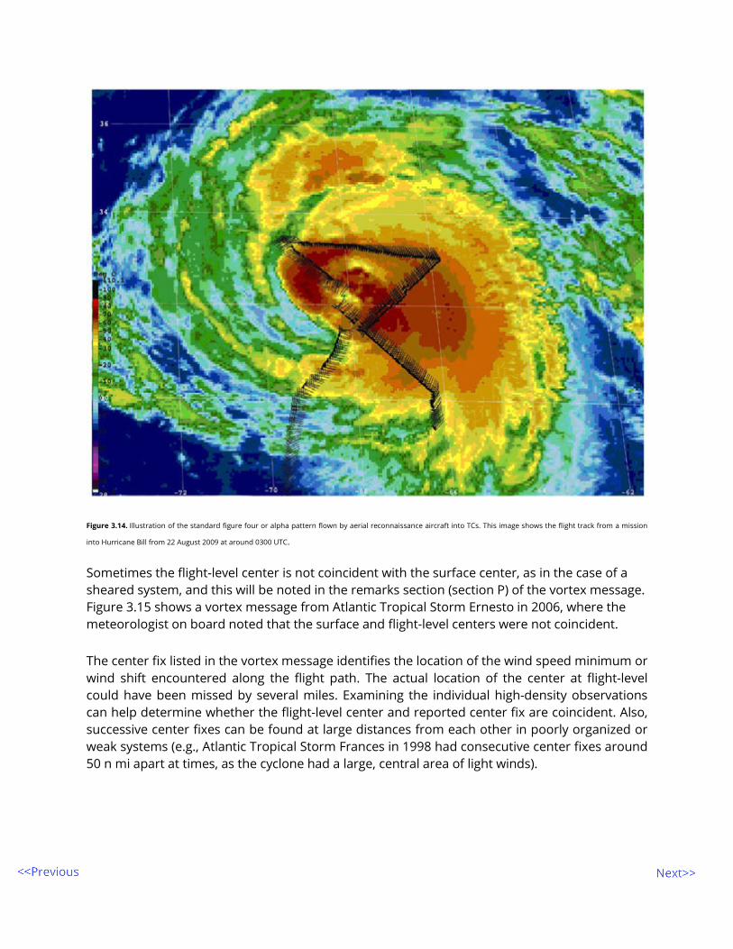
Figure 3.14. Illustration of the standard figure four or alpha pattern flown by aerial reconnaissance aircraft into TCs. This image shows the flight track from a mission

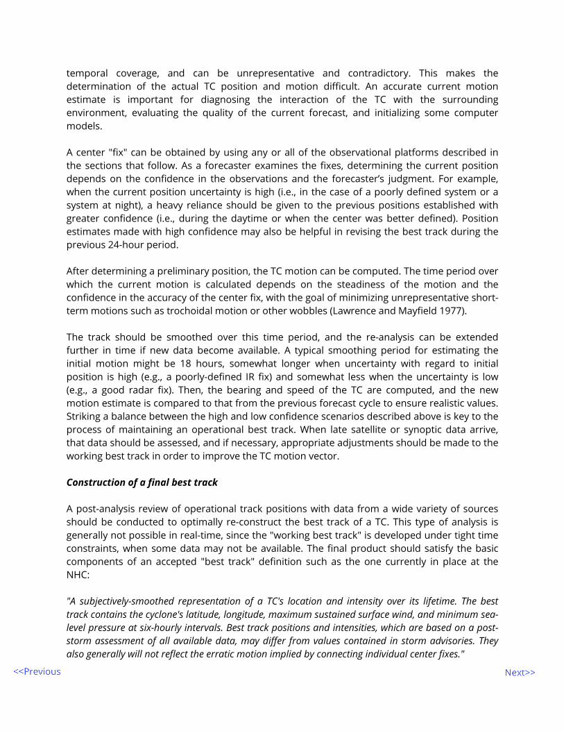
into Hurricane Bill from 22 August 2009 at around 0300 UTC. Sometimes the flight-level center is not coincident with the surface center, as in the case of a sheared system, and this will be noted in the remarks section (section P) of the vortex message. Figure 3.15 shows a vortex message from Atlantic Tropical Storm Ernesto in 2006, where the meteorologist on board noted that the surface and flight-level centers were not coincident. The center fix listed in the vortex message identifies the location of the wind speed minimum or wind shift encountered along the flight path. The actual location of the center at flight-level could have been missed by several miles. Examining the individual high-density observations can help determine whether the flight-level center and reported center fix are coincident. Also, successive center fixes can be found at large distances from each other in poorly organized or weak systems (e.g., Atlantic Tropical Storm Frances in 1998 had consecutive center fixes around 50 n mi apart at times, as the cyclone had a large, central area of light winds).

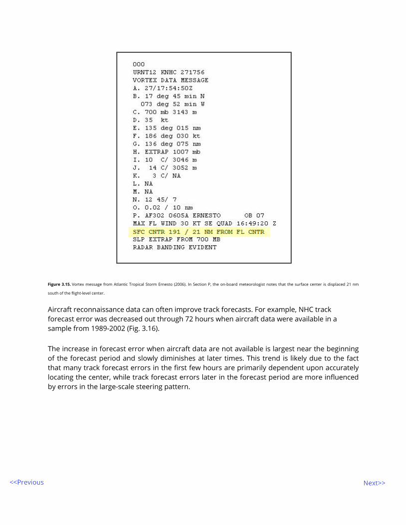
Figure 3.15. Vortex message from Atlantic Tropical Storm Ernesto (2006). In Section P, the on-board meteorologist notes that the surface center is displaced 21 nm

south of the flight-level center. Aircraft reconnaissance data can often improve track forecasts. For example, NHC track forecast error was decreased out through 72 hours when aircraft data were available in a sample from 1989-2002 (Fig. 3.16). The increase in forecast error when aircraft data are not available is largest near the beginning of the forecast period and slowly diminishes at later times. This trend is likely due to the fact that many track forecast errors in the first few hours are primarily dependent upon accurately locating the center, while track forecast errors later in the forecast period are more influenced by errors in the large-scale steering pattern.

Figure 3.16. NHC official forecast errors with and without reconnaissance data, 1989-2002. The percent improvement in track error when aircraft data were available is

indicated in parentheses. urveillance missions An accurate representation of large-scale steering features in the TC environment and their interaction with TCs is critical to TC track forecasting. Acquisition of wind, geopotential height, and thermodynamic observations in the often data-sparse TC environment is helpful in accomplishing this goal. Air Force reconnaissance aircrews often flew "synoptic" missions from at least from 1974 to 1987 in the western North Pacific to assess mid-tropospheric ridge structure in order to ascertain the likelihood of recurvature or non-recurvature (Guard, personal communication). NOAA's Hurricane Research Division (HRD) flew a large number of "synoptic flow" missions near and around TCs in the Atlantic between 1982 and 1996, and these data resulted in significant reductions in forecast errors (Burpee et al. 1996). Improvements depend greatly on the amount of data coverage but have been on the order of 10-15% in critical watch/warning situations from 1997-2006 (Aberson 2010). These research flights led to

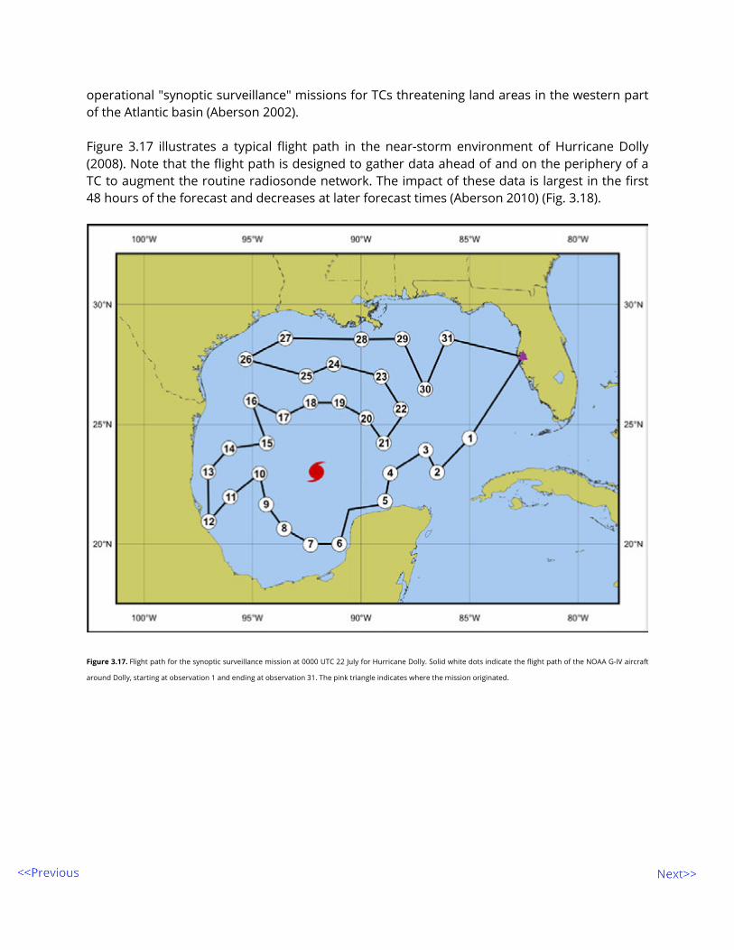
operational "synoptic surveillance" missions for TCs threatening land areas in the western part of the Atlantic basin (Aberson 2002). Figure 3.17 illustrates a typical flight path in the near-storm environment of Hurricane Dolly (2008). Note that the flight path is designed to gather data ahead of and on the periphery of a TC to augment the routine radiosonde network. The impact of these data is largest in the first 48 hours of the forecast and decreases at later forecast times (Aberson 2010) (Fig. 3.18).

Figure 3.17. Flight path for the synoptic surveillance mission at 0000 UTC 22 July for Hurricane Dolly. Solid white dots indicate the flight path of the NOAA G-IV aircraft

around Dolly, starting at observation 1 and ending at observation 31. The pink triangle indicates where the mission originated.

Figure 3.18. Average track errors (km) for a homogeneous sample of GFS model runs and a homogeneous sample of GFDL model runs, with (ALL) and without (NO)

surveillance data initialized only at mission nominal times, and improvements over the former and not the latter (%). Sample sizes for each model at each forecast time

are provided above the graph. Reproduced from Aberson (2010). Radar fixes The use of radar provides another data source to fix the center of TCs nearing land. As a TC approaches a radar site, outer rainbands, some of which move ahead of and at roughly the same speed and direction as the cyclone, appear first. While determining an accurate center location by radar is not possible at this stage, fitting logarithmic curves with a constant crossing angle of 10°-20° can provide an initial indication of the cyclone center once significant lengths of spiral band are observed (Senn and Heiser 1959). Once an eye or distinct circulation center appears, radar can provide center fixes with high temporal frequency. The accuracy of these

fixes can approach or exceed those of aircraft reconnaissance. However, the precision of the center fixes varies with the range and intensity of the TC due to the Earth's curvature and greater uncertainty associated with interpreting reflectivity patterns at long ranges from the radar site. Figure 3.19 shows a scatter of radar fixes at a distance from the radar, when Tropical Storm Fay was poorly organized between Cuba and south Florida. As Fay intensified and the center became better defined, the scatter in fix positions decreased. Radar images can be animated to maximize the utility for centering fixing. Due to refraction of the radar beam and the Earth's curvature, considerable resolution and information are lost as the distance from the radar increases. The effect of the increase in height of the beam with increasing range is illustrated in Figure 3.20, where it appears that little deep convection exists on the southwest side of the eyewall. However, the lack of deep convection southwest of the eye is likely a result of the radar beam overshooting the largest hydrometeors associated with the convection in that area.

Figure 3.19. Operational radar center fixes plotted for Atlantic Tropical Storm Fay (18-21 Aug 2008) as it traversed the Florida peninsula. Scatter in the early land-based

radar fix positions is strongly a function of distance from the radar and strength of the system. Smoothed best-track positions are overlaid, along with a radar image

from the Key West WSR-88D (KBYX) from 1811 UTC 19 Aug.

Figure 3.20. Atlantic Hurricane Lenny (0212 UTC 17 Nov 1999) south of Puerto Rico. The effect of the increased height of the beam above the surface with increasing

range is demonstrated. Range rings indicate the height of the center of the radar beam above the surfac The basic center-fixing technique is to find the geometric center of the eye (which may be circular or elliptical). Significant errors can occur when the eye is ragged or only formed on one side (Meighen 1987). In these circumstances, the eye wall feature should be found by animating the radar images and maintaining a conservative size and shape of the eye over several hours. In addition to reflectivity data, Doppler radar can measure whether backscattering particles are moving towards or away from the radar (i.e., radial velocity). Two Doppler radars in close proximity can provide full three-dimensional winds in regions where their beams overlap at an appropriate angle. An airborne Doppler radar can also obtain a full wind field by sampling the same volume from different locations.

The use of single-Doppler velocities in conjunction with the reflectivity (Fig. 3.21a) can greatly increase the accuracy of a radar-determined center fix. The zero isodop (Figure 3.21b), indicating particle motion normal to the beam, establishes the bearing of the TC center from the radar. The wind center will lie on or near the zero isodop, assuming that the component of TC motion towards or away from the radar is small. Although the TC center will be found between the inbound and outbound radial velocity maxima, the center observed by radar is at some distance above the surface. If data from adjacent radars are also available, multiple estimates of zero-isodops can help to refine or confirm a center fix, particularly in weaker systems. A reflectivity mosaic from multiple radar sites can also be helpful in identifying the center.

Figure 3.21. Radar reflectivity image of Hurricane Dennis at 1835 UTC 10 July 2005, as it approaches the Gulf coast of Florida. The radar location is indicated by white

dot. b) corresponding velocity image, with "x" indicating center fix. Note inbound velocity maximum (dark blue) and outbound maximum (yellow) falling on either side

of the zero “isodop” (gray) (counter-clockwise flow, northern hemisphere). Maximum velocity in this image is 56 ms-1 (109 kt) inbound at an altitude of about 2400 m

(8000 ft).

Land observations and ship reports Surface observations are not dense enough to accurately track a TC center, especially over the open oceans. However, surface observations can be important, particularly if they are located near the TC center. For example, an unexpected ship report can sometimes confirm the presence or location of a TC center in an otherwise data-void area. The wind speed and direction from surface observations give some indication of how far from and in what direction the TC lies from the observing site, while the pressure tendency helps to determine whether the TC is moving toward or away from the site. A time series of surface observations updated with regular frequency is more valuable than a single observation. Veering or backing of the wind direction with time indicates whether the TC center is approaching or moving away from a location, respectively. Unfortunately, most ship reports are made only at 3- or 6-hourly time intervals. First-order land sites and mesonets, coastal stations, and buoys report hourly, but some stations may have data interruptions due to power outages, communication failures, and even station destruction in more severe TCs. Also, the representativeness of surface

observations should be considered to ensure that transient features within the TC circulation have not contaminated the data. There has been an expansion of land and ocean observations in recent years from a variety of new sources. For example, the number of coastal mesonets and other buoy networks over different parts of the globe has rapidly increased. Figure 3.22 shows the relatively high density of observations in the vicinity of the Florida peninsula. Some university research groups coordinate the deployment of observing networks in the path of a TC to supplement observations available at a TC la

Figure 3.22. Map showing a subset of the large number of coastal observations in the vicinity of the Florida peninsula in the southern United States. Sustained winds are greatly influenced by exposure and surface roughness characteristics. A better measure of tropical cyclone sustained wind is frequently obtained by using the observed gust and then converting it to an associated sustained wind as determined from a general relationship that better pertains to winds observed in tropical storms and hurricanes (e.g., Krayer and Marshall 1992; Harper et. al. 2010).

An observed coastal, island, buoy or ship wind is often interpreted as the "'maximum' maximum" wind at that distance from the center (e.g.,radius of maximum wind, or radius of 15 ms-1 wind). However, it should be interpreted as the "minimum maximum" wind. Why? Because there is very little chance that the sampled wind is located exactly at the point of the peak wind at that distance. While there are various geometric techniques that can be used to estimate the location of the TC center from synoptic data at various locations, satellite techniques are now more accurate and render these techniques obsolete. Techniques for operationally combining and weighting various types of data are covered by Powell (XXXX).

3.3 TC track forecasting

Factors influencing TC motion

Large-scale flow Fundamentally, TC motion is governed by two mechanisms: advection of the relative vorticity associated with the TC by the environmental flow, and advective processes that involve multi-scale interactions on different scales with the environmental flow, the planetary vorticity gradient, and the TC vortex. In the first mechanism the TC is analogous to a "cork moving in a stream," where the layer-averaged winds over the depth of the troposphere correlate well with the actual storm motion, indicating the dominance of the environmental steering mechanism. A forecaster can develop a simple estimate of the deep-layer steering, which could serve as a proxy for the actual TC motion. The calculation for this parameter is known as the deep-layer mean (DLM) wind and is simply the mass-weighted average wind through some layer of the troposphere. For example, if the vertical layer extends from 850 hPa to 200 hPa, the vertical integration can be approximated by the following expression:

[(U850+U500)/2 * 350 mb + (U500+U200)/2 * 300 mb)] / (650 mb)

Neumann (1979) examined the relationship between deep-layer mean heights and TC motion and determined that geopotential height works equally well as using layer winds. He also discovered that layer-averaging was more preferable than using a single layer and determined that a mass-weighted average extending from near the surface to 100 hPa explained the greatest variance of short-term TC motion. An empirical relationship exists between the intensity of the TC and the vertical depth of its vortex in the troposphere (Velden & Leslie 1991 and Velden 1993). Therefore, a forecaster should consider the intensity of a TC before determining the appropriate steering layer to consider. Figure 3.23 indicates that stronger TCs typically extend through the depth of the troposphere and are steered by a DLM wind. Weaker storms typically have less vertical depth, and a shallower layer of average winds should be examined to assess the potential TC motion.

The forecaster can use this concept to compare the vertical depth of the vortex in model output to ensure that the model has the proper representation of the TC. If a TC is sheared to the point that the low-level circulation center and the deep convection become decoupled, the sheared low-level center will generally be steered by the 850 hPa or 850-700 hPa mean flow.

Figure 3.23. Relationship between TC intensity and TC environmental steering from Velden (1993). Bars indicate the depth of the steering layer in hPa (y-axis) and TC

intensity is given on the x-axis.

Figure 3.24 shows the forecast scenario at 0600 UTC 5 September 2008, when Hurricane Ike was centered well east of Florida. A majority of the track guidance at that time indicated that Ike would turn from a west-southwest course north of Puerto Rico to a west-northwest or even northwest course later in the forecast period.

Figure 3.24. Model track guidance for Hurricane Ike at 0600 UTC 5 September 2008. The solid white line with hurricane symbols represents the best track, while the

multi-colored lines represent individual track model forecasts out to 3 days; multi-colored, dashed lines represent individual track model forecasts from 3 to 5 days. The

cyan track is the official forecast, the black line is the GFS model, and the orange line is the ECMWF model. A series of cross-sections from the GFS, one of the models forecasting a northwesterly course beyond 72 hours, appears in Figure 3.25a. These cross-sections show that the GFS depicts Ike as a shallow vortex, with little circulation evident above about 500 hPa, even though Ike was a hurricane at the initial time. Many of the other models also forecasting a northwesterly course suffered from poor model representations of the TC vortex, indicating a weak TC throughout the forecast period (not shown). In contrast, the ECMWF (Fig. 3.25b) shows a deeper TC vortex consistent with a mature hurricane. The ECMWF model, with its more accurate depiction of Ike's vortex, consistently forecast the hurricane to remain farther south, closer to the eventual track. This result suggests that Ike was being steered by a deep layer mean (DLM) flow from the northeast around a strong subtropical high to the north (Fig. 3.26b). The GFS, however, steered its weaker representation of Ike in shallower flow around the low- to mid-level Atlantic ridge (Fig 3.26a).

Figure 3.25. Forecast east-to-west model cross-sections for Hurricane Ike. GFS's (a) and ECMWF's (b) analyses and forecasts through 48 h of relative vorticity and

horizontal winds (every 6 hours) associated with Hurricane Ike from model cycles at 0600 UTC 6 September and 0000 UTC 6 September, respectively. A horizontal

distance across the TC is on the x-axis, while pressure (in hPa) is indicated on the y-axis. Vorticity is shown in units of x 10-5

m2

s-2

, with the red and purple shading

indicating positive vorticity and blue shadings indicating negative vorticity. Forecast wind barbs are displayed in knots.

Figure 3.26. Analysis at 0000 UTC 9 September 2008 from (a) GFS showing sea level pressure (contours, hPa) and 850-500-hPa layer average wind (barbs, kt), and (b)

ECMWF showing sea level pressure (contours, hPa) and 850-200-hPa deep layer mean (DLM) wind (barbs, kt).

Beta-gyres The beta effect represents a form of self-advection and results from differential advection of planetary vorticity on either side of the TC circulation. The differential advection induces weak

secondary circulations known as “beta gyres” on either side of the TC, which cause a net westward and poleward drift of about 1-2 ms-1. Observing beta gyres in nature is virtually impossible, as their effects are manifest as a subtle modification to the large-scale steering flow. The beta effect is dependent on the outer wind structure of the TC, a part of the storm that is often poorly sampled even by reconnaissance aircraft (Carr and Elsberry 1997). The Beta and Advection Models (BAMs) are simple, two-dimensional trajectory models that contain vertical layer-averaged horizontal winds in addition to a correction term that accounts for the beta effect. In fact, most contemporary dynamical models incorporate the effects of beta-gyres. Thus, while forecasters should be aware of this contribution, under most conditions, they need not calculate it. Binary interaction The interaction of two or more closely-spaced TCs can lead to what is known as the Fujiwhara effect (Fujiwhara 1921, 1923, 1931; Brand 1970) or binary interaction (Dong and Neumann 1983). Fujiwhara (1921, 1923, 1931) explains how similar-sized cyclones are mutually attracted to one another and orbit cyclonically about a mid-point. Brand (1970) showed that TCs begin to interact significantly when their centers come within 700-800 nm (1125-1290 km) of each other. The degree of interaction increases rapidly as the distance between the cyclones decreases. The details of the interaction also depend on storm size, intensity, and the ambient steering flow, with storms of unequal sizes likely to have a greater interaction than two of the same size (Prieto et al. 2003). Once two TCs come into proximity, there are several possible outcomes: the two TCs could move in a stable, cyclonic orbit about their centroid; one cyclone could escape the interaction of the other; or one of the cyclones could dissipate via capture and merger. The absorption of one TC by another is relatively rare and is most likely to occur when one cyclone is much larger and stronger than the other (Lander and Holland 1993). For example, Tropical Storm Henriette in the eastern North Pacific in 2001 dissipated after coming within 85 km of Tropical Storm Gil, after having already rotated about 540 degrees around their centroid (Prieto et al. 2003). Ritchie and Holland (1993) found that vortices must come within 150-300 km of each other before a "shearing-out" process can occur which can ultimately lead to dissipation of the smaller of the two vortices. Binary interactions are most prevalent in the western North Pacific since TCs there are in relative greater abundance of multiple cyclones and the characteristics of the monsoon trough environment favor multiple opportunities for TCs to encounter one another (Dong and Neumann 1983). Atlantic TCs generally form from individual perturbations (African Easterly Waves) outside of the ITCZ and have fewer chances to undergo binary interaction (Dong and Neumann 1983). Dong and Neumann (1983) also found that the expected annual number of binary interactions in the western North Pacific is 1.5, considerably higher than the 0.33 expected annually in the Atlantic. When normalized with respect to total storm numbers, however, the western North Pacific experiences about the same amount as most other global basins, except for the Atlantic basin, which experiences the lowest amount.

Track forecasting becomes more difficult when considering the interactions of two or more TCs (Dong and Neumann 1983). Carr and Elsberry (1998) presented a detailed conceptual model that classifies binary interaction events by the degree of interaction between storms (direct, semidirect, and indirect), the dominance of one system over another, a cyclone's interaction with neighboring steering features, or the mean steering flow. Unfortunately, the scheme is qualitative in practice and can fail to detect binary interaction or delay its detection. From the forecaster's perspective, binary interaction can be masked by the influence of the environmental flow, making its onset difficult to determine. Contemporary numerical models can better resolve TCs and handle binary interaction better than they did a decade or two ago, although no systematic study has assessed model forecast skill in these cases. Model forecasts should be evaluated to determine if they properly analyze the location, intensity, and size of the TCs involved in binary interaction, since a failure to correctly analyze any of these parameters could result in a degradation of details of the binary interaction depicted in the model forecast. All of the parameters are critical to properly resolve the timing and degree of binary interaction. Differences between various models can be compared to see if the interaction shown in the model is consistent with previous studies. TC interaction with surrounding environment Interactions between a TC and the surrounding environment are also important to TC motion (Ross and Kurihara 1995). Large, strong TCs have a more significant effect on the surrounding environment than smaller, weaker ones, and this environmental modification could influence TC motion. One example is the transport of heat by upper-level outflow poleward of a TC, which could enhance a mid- to upper-level anticyclone and keep the TC on a general westward heading. The Beta Effect discussed above is another example of a TC environmental interaction. TC motion can also be affected by terrain interaction; however, the details of this interaction vary with the strength of the TC, the strength and direction of the actual environmental steering, and the characteristics of the terrain. Observational and numerical studies have demonstrated that an acceleration and significant poleward track deflection can occur upstream of a rugged land mass (e.g., like Taiwan) for westward-moving TCs (Brand and Blelloch 1974; Chang 1982; Bender et al. 1987; Yeh and Elsberry 1993). These same studies also show that stronger TCs tend to have more continuous tracks across mountainous islands while weaker TCs tend to "jump" or reform a secondary circulation on the lee side of elevated terrain through the conservation of potential vorticity. Similar track deflections have also been observed in TCs passing over other islands such as Cuba, Hispañiola, Puerto Rico, and Luzon in the Philippines (Lin et al. 2006). The low-level circulation center of TCs approaching the north-south oriented Sierra Madre mountain range of eastern Luzon in the Philippines tends to: 1) cross the mountain range if the environmental steering has a greater westward than northward component; or 2) move northward east of the mountain range if the environmental steering has a greater northward component than westward component (Guard, personal communication). TC core processes that influence motion

Several "secondary" mechanisms also produce TC track oscillations. Holland and Lander (1993) discuss how TCs tend to oscillate about a mean path, even if they are in a particularly well-defined steering current. Willoughby (1988) demonstrated that a mass source and sink couplet exhibited trochoidal oscillations along the cyclone path, such as those documented in Atlantic Hurricane Belle in 1976 by Lawrence and Mayfield (1977). Willoughby (1984, 1990) and Holland and Lander (1993) further discuss the role that convective asymmetries, such as mesoscale convective systems rotating within the core of the TC, can have on short-term TC motion. Ritchie and Elsberry (1993) acknowledge the possibility that significant track changes on the order of tens to even hundreds of kilometers over several days could result from the interaction of a TC and a persistent MCS rotating within its circulation. Even in cases of land interaction, changes in TC motion are sometimes related to convective asymmetries within the storm due to asymmetric surface fluxes and frictional effects (Wong and Chan 2006). Models and forecasters have not been able to routinely predict convectively-related "jumps" or reformations of the center observed in TCs. In the case of Tropical Storm Claudette on 12 July 2003, the center, which was located over the central Gulf of Mexico, unexpectedly jogged north of the forecast track. Claudette was embedded in a persistent southwesterly shear environment, which caused the bulk of the convective activity to be distributed asymmetrically north and northeast of the center. This is consistent with Ritchie and Elsberry (1993) who found that a persistent burst of convection, especially in an asymmetric pattern, can cause a localized pressure fall through latent heat release and an increase in the vertical vorticity through the divergence term in the vorticity equation, resulting in a "jump" or reformation of the center. In the case of Claudette, the convective asymmetry appeared to tug the center northward throughout the day, with the center eventually reforming closer to the deepest convective cells several hours later. Neither forecasters nor the track guidance anticipated this motion, and the likelihood of being able to forecast short-term track motion with a time scale of this type of convective asymmetry is low. If an asymmetric convective pattern is expected to persist, the forecaster may be able to deviate from the track guidance (Ritchie and Elsberry 1993), however, extrapolating a short-term motion too far into the future, especially after the initial forcing agent has dissipated, is not advisable. The important aspect for the forecaster is to recognize the potential for a change in motion so that when it occurs, he or she does not go into an extended period of denial (i.e., not believing what they are seeing). Tools for TC track forecasting Climatology There are some motion characteristics of TCs that occur regionally and seasonally. For example, late season TCs in the Atlantic basin tend to form over the western Caribbean Sea and accelerate northward or northeastward. Storm-specific information such as the location, current motion, day of the year, and intensity of a TC can be compared to historical TCs with similar characteristics through linear regression to develop a "climatology-persistence" (CLIPER)

model that identifies a "typical" storm behavior. As forecasts from dynamical models have improved, the operational use of simple statistical models such as CLIPER for track forecasting has declined sharply. Since the CLIPER technique contains no information about the current state of the atmosphere, its use, especially at longer time ranges, is rather limited and it is no longer an effective forecast tool, but such information could be used as a long-term planning tool. Apart from its limited use in an operational setting, CLIPER or similar methods serve as a benchmark against which the performance of dynamical models can be evaluated (Aberson 1998, Bessafi et al. 2002). Since CLIPER contain no information about the current state of the atmosphere, it represents a "no skill" forecast. Forecasts from other techniques, including the official forecast, can be evaluated against CLIPER to quantify the amount of skill they have. In addition, if CLIPER errors for a particular TC or an entire season are low (high), the interpretation can be made that the storm(s) were inherently easier (more difficult) to forecast than normal. This concept of forecast difficulty has been normalized to rank basins according to their general forecast difficulty (Pike and Neumann, 1987). Persistence TC motion is determined mostly by the large-scale steering flow. If the flow in which a TC is embedded is gradually evolving, persistence can be important in forecasting TC track in the first 12 to 24 hours. At these short time periods, extrapolation of the TC's past track can be used to determine future position. Beyond that time, steering mechanisms and their non-linear interactions become complex and TC track is best predicted using dynamical model guidance. In order to use persistence, a forecaster must determine a representative estimate of TC motion. The initial motion is typically computed with an averaging period over the past 6, 12, 18, or even 24 hours. An interval of 6 to 12 hours is best if known changes in the track are occurring (e.g., recurvature), but a longer interval may be chosen if the center location is uncertain. In general, the time interval for averaging can be thought of as a smoothing factor, with more smoothing and a longer averaging time necessary for TC centers that are difficult to fix. Continuity Maintaining continuity with the previous forecast should be a priority in the forecast process. Small, incremental changes are typically made to the forecast from cycle to cycle in an attempt to avoid following the sometimes abrupt changes in track model guidance (e.g., Figs. 3.29-3.32). If forecast changes are not constrained by continuity, large changes in one direction may have to be adjusted significantly back in the other direction shortly thereafter. It is important to avoid large changes to the forecast track since they could cause the public and other users to lose confidence in the official forecast. The forecaster should instead strive for gradual changes from one forecast to the next following trends in the guidance. However, there are occasionally situations when large changes to the forecast track are required, such as the reformation of the center or a significant, unexpected deviation from the previous forecast motion.

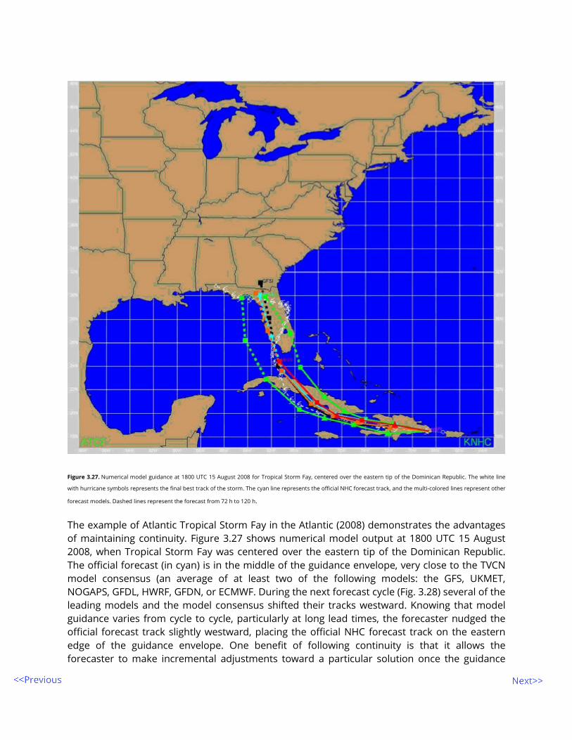
Figure 3.27. Numerical model guidance at 1800 UTC 15 August 2008 for Tropical Storm Fay, centered over the eastern tip of the Dominican Republic. The white line

with hurricane symbols represents the final best track of the storm. The cyan line represents the official NHC forecast track, and the multi-colored lines represent other

forecast models. Dashed lines represent the forecast from 72 h to 120 h. The example of Atlantic Tropical Storm Fay in the Atlantic (2008) demonstrates the advantages of maintaining continuity. Figure 3.27 shows numerical model output at 1800 UTC 15 August 2008, when Tropical Storm Fay was centered over the eastern tip of the Dominican Republic. The official forecast (in cyan) is in the middle of the guidance envelope, very close to the TVCN model consensus (an average of at least two of the following models: the GFS, UKMET, NOGAPS, GFDL, HWRF, GFDN, or ECMWF. During the next forecast cycle (Fig. 3.28) several of the leading models and the model consensus shifted their tracks westward. Knowing that model guidance varies from cycle to cycle, particularly at long lead times, the forecaster nudged the official forecast track slightly westward, placing the official NHC forecast track on the eastern edge of the guidance envelope. One benefit of following continuity is that it allows the forecaster to make incremental adjustments toward a particular solution once the guidance

begins to consistently predict a given scenario, while avoiding drastic changes. The track models shifted back toward the east (Fig. 3.29) at 0600 UTC 16 August, closer to the original set of guidance from 12 hours before, and the forecaster made only a minor adjustment to the official forecast track.

Figure 3.28. As in Fig. 3.27, except for 0000 UTC 16 August 2008, when Tropical Storm Fay was near Santo Domingo, Dominican Republic.

Figure 3.29. As in Fig. 3.27, except for 0600 UTC 16 August 2008.

Figure 3.30. As in Fig. 3.27, except for 1200 UTC 16 August 2008. Model guidance continued shifting eastward at 1200 UTC 16 August (Fig. 3.30), and the forecaster, now detecting a possible trend, shifted the track more significantly eastward. The official NHC track deviated little from the 1200 UTC forecast track during the next several cycles as the model guidance converged on a solution. In this case, if the forecaster had not considered continuity and had shifted the track farther westward at 0000 UTC 16 August, the eastward shift in the model guidance at subsequent forecast times would have required major changes to the forecast. Beta and Advection Models (BAM) BAM refer to a class of simple trajectory models that use vertically-averaged horizontal winds to produce TC trajectories, while adding a beta correction term to account for the Earth's rotation. These models use different layer means and can be used to assess likely storm motion in different situations: BAM shallow (850-700 hPa), BAM medium (850-400 hPa), and BAM deep

(850-200 hPa), known as BAMS, BAMM and BAMD, respectively. For example, for a weak or severely sheared system the BAMS output would be a better indicator of TC motion than BAMD, especially when the environmental flow is simple and baroclinic forcing is weak. Global models Many forecasting agencies such as the European Center for Medium-Range Weather Forecasts (ECMWF), the U.S. National Weather Service (NWS), and the U.K. Met Office (UKMET) operate central facilities that run numerical weather prediction models at least twice daily out to as long as 15 days. While global dynamical models were not designed to explicitly predict TC track, they have demonstrated increasing skill in this area due to improved forecasts of the large-scale steering flow that controls TC motion. Also, their lack of lateral boundary conditions in global models means that their performance at longer ranges is more skillful than regional models. In fact, global models are the best TC track forecast guidance, especially beyond 48-72 h. A significant challenge to TC modeling has been developing a method by which the relatively small-scale TC vortex can be properly analyzed by relatively coarse models in regions with little data. In the NOGAPS and UKMET global models, a method to construct a TC vortex by using "bogus" or synthetic observations is utilized. Another scheme known as "vortex relocation" is utilized in the GFS model, which does not modify the analyzed TC vortex but repositions it to the official position estimate, resulting in more accurate forecasts by that model. Elsberry (2005) found that the GFS model 72-hour average track error decreased considerably, to 193 nm after the inclusion of this procedure from 2000-2003; an astonishing increase in forecast skill of 42% with respect to CLIPER. However, the ECMWF global model, which uses neither scheme, has emerged as one of the more skillful track models in the Atlantic in recent years. For additional information on the vortex relocation procedure, refer to Liu et al. (2000), Gao et al. (2010) or Hsiao, et al. (2010). Regional models

Dynamical models designed specifically for TCs (e.g., GFDL, GFDN, and HWRF) are known as limited-area or regional models. Their limited areal coverage means that they can have higher horizontal and vertical resolution, which is an important factor in the accurate depiction of TC structure for intensity forecasts. In the GFDL, the vortex is "spun up" in a separate model and inserted into the model analysis at the initialization time. The more explicit representation of the TC also means that regional models can handle interactions better between the TC and its environment, which can result in improved short-term track forecasts. However, a disadvantage to the limited model domain is that critical upstream weather features may initially be located outside the model domain and may be handled poorly in the model forecast (M. Bender, personal communication). As a result, the skill of regional models for track beyond a few days is less than that of the global models (Franklin 2009). For example, the GFDL model performs well through 48 h followed by a severe degradation in forecast skill by 120 h (Fig 3.31). Ensembles

An ensemble is a collection of model forecasts verifying at a common time. Ensembles are generally composed of multiple model forecasts, typically from the same model using small changes (i.e., perturbations) in the initial conditions to represent the uncertainty in the analysis. These initially small perturbations grow with time and in a perfect ensemble, the truth would always lie within the envelope of possible ensemble solutions. Most global ensemble systems are run with 20 or more member forecasts with somewhat coarser resolution than their global deterministic model counterparts. Other ensembles are created by varying the formulation of the model itself. Also, a collection of forecasts from different models is another way to construct an ensemble. While global model ensembles are most frequently used for large-scale pattern forecasting, they can be useful for longer-term TC track forecasting, particularly for diagnosing trends in the large-scale circulation patterns that can govern TC motion. However, up to this time, the average forecast skill of the ensemble mean of both the U.S. Global Ensemble Forecast System (GEFS) and the ECMWF ensemble system through five days has not surpassed that of their counterpart deterministic global models in the Atlantic or East Pacific (Franklin 2010). More detailed overview of the use of ensembles in TC track forecasting can be found at Heming & Goerss (2010). Further examples are presentations at ITWC VII by Foley (2010) and Nakazawa (2010).

Table 3.2 presents basic model specifications and other characteristics. Heming & Goerss (2010) provides a detailed description of specific global models and descriptions of individual ones primarily used for TC track prediction. Note that NWP development is ongoing, these specifications were current about 2009. Table 3.2. Operational models in use at NHC. Timeliness is given as "E" for early and "L" for late. & Canadian GEM model uses a 4D-VAR scheme that makes use of in

situ flight data.

Name/Description ATCF

ID Type Resolution

Vortex Specification

Timeliness

NWS/Geophysical Fluid Dynamics

Laboratory (GFDL) model

GFDL Multi-layer

regional dynamical

Inner grid 5°x5° at 1/12° spacing, intermediate grid

11°x11° at 1/6° spacing, outer grid 75°x75° at 1/2° spacing, 42 vertical levels

Synthetic vortex

L

NWS/ Hurricane Weather Research

and Forecasting Model (HWRF)

HWRF Multi-layer

regional dynamical

9x9km, 42 vertical levels Synthetic

vortex L

NWS/Global Forecast System

GFS Multi-layer

global T382L64, (~35 km

horizontal resolution)/td> Vortex

relocation L

(GFS)

National Weather Service Global

Ensemble Forecast System (GEFS)

AEMN Consensus T190L28 (0-180h) Vortex

relocation L

United Kingdom Met Office model

(UKMET) UKM

Multi-layer global

dynamical (Grid point)

0.5°x 0.4° (~40 km at mid-latitudes)

Bogussing L

Navy Operational Global Prediction System (NOGAPS)

NGPS

Multi-layer global

dynamical (Spectral)

T239L30(approximately 55 km horizontal resolution)

Bogussing L

Navy version of GFDL

GFDN Multi-layer

regional dynamical

Inner grid 5°x5° at 1/12° spacing, intermediate grid 11°x11v at 1/6° spacing,

outer grid 75°x75° at 1/2° spacing, 42 vertical levels

Synthetic vortex

L

European Center for Medium-range Weather Forecasts

(ECMWF) Model

EMX Multi-layer

global dynamical

T1279L91 (approximately 16 km horizontal

resolution)

No vortex specification

L

Environment Canada Global Environmental

Multiscale Model

CMC Multi-layer

global dynamical

33 km (~45°N) horizontal resolution, 58 vertical

levels

4-D VAR scheme&; no

bogus L

Beta and advection model (medium

layer) BAMM

Single-layer trajectory

T25 resolution No vortex

specification E

Beta and advection model(deep layer)

BAMD Single-layer trajectory


specification E

Beta and advection model (shallow

layer) BAMS

Single-layer trajectory


specification E

NCEP North American Model

NAM Multi-layer

regional dynamical

12km horizontal, 60 vertical levels

No bogus E

Consensus-based approach No single model is consistently the best at forecasting TC track. The relative reliability of the models fluctuates from season to season due to changes in resolution, physical paramterizations, or data assimilation schemes. Fluctuations in model performance can also be seen from one run to the next due to errors in model initial conditions and how individual models handle critical features, including the TC itself. A forecast derived from inputs from different models is often referred to as a "consensus" forecast. The simplest consensus is just an average (or mean) of the forecasts from the individual member models. Grouping several independent models together to form a multi-model ensemble can provide a more skillful forecast than an individual model. Goerss (2000) illustrated the value of a consensus-based approach by forming a simple model consensus of three global models and another consensus of two regional models. The track errors of both consensus models were significantly smaller than those from the best individual models. The addition of new models to the consensus generally leads to minor but steady gains in skill, especially if the number of models in the consensus is small since the effectiveness of a model consensus relative to each individual member is a function of the independence or effective degrees of freedom of the models forming the consensus. In fact, the inclusion of a model that is less skillful than the other consensus members can still yield a positive contribution. Sampson et al. (2006) showed that the inclusion of a relatively simple barotropic model in the consensus produced a large positive impact in spite of that model’s generally larger errors. A larger consensus produces smaller mean errors by reducing the influence of large errors from any individual model, especially when the degree of independence is high. The error reductions that occur when different models are combined are demonstrated in Figure 3.31 where the GUNA consensus, an average of the GFDL, UKMET, NOGAPS, and GFS models, outperforms not only all of the models it comprises but also the GEFS ensemble mean. Rappaport et al. (2009) note that the GUNA consensus outperformed the most skillful of all the GUNA constituents, the GFDL model, by 18% between 2004 and 2006. A dynamical model consensus is often an excellent starting point in the preparation of the track forecast and is difficult to beat as a final forecast, after accounting for continuity.

Figure 3.31. Skill of individual and consensus models for TC track in the Atlantic from 2005-2009 relative to CLIPER. The number of cases is indicated in black at each

time interval.

The building of a consensus must take into account model availability, which can differ considerably from model to model. "Fixed" consensus solutions require that all members of the consensus be available before computing the model consensus (e.g., GUNA); others, like the "variable" consensus models require a minimum of two available members (e.g. TVCN, an average of at least two of the GFS, ECMWF, NOGAPS, UKMET, GFDL, GFDN, and HWRF). The greater number of consensus members increases the chance of having the minimum number of models available to generate a consensus forecast for a variable consensus model. However, this can lead to consistency issues, when, for example, the 120-hour forecast in a variable consensus may be based on a different set of models than the 96-hour position. Corrected consensus scheme Another technique is the "corrected" consensus, which is formed by computing statistical correctors for the member models based upon parameters that are known at the time the forecast is made. These correctors come from regressing model tracks against the "best track" and then assigning weights to each member model solution based on that model's past performance (Vijaya Kumar et al. 2003). Corrections can be based upon the previous model

biases, current model spread, the initial TC position, intensity, and the forecast track. The corrected consensus can be computed in real time or updated annually (Weber et al. 2003). The FSU Superensemble is an example of the corrected consensus technique. The corrected consensus approach requires a large sample of retrospective runs to develop robust statistics for the bias correction. However, since models are updated frequently, the bias corrections developed may not be applicable to modified versions of the model or the corrections may not be drawn from a large enough sample. Drawing conclusions about storm behavior from an insufficient number of cases is not advisable, since meteorological conditions in small sample are not varied enough to be representative (Franklin 2009). As a result of this limitation, the corrected consensus approach has not shown improvement over the simple consensus methods. Sustained winds are greatly influenced by exposure and surface roughness characteristics. A better measure of tropical cyclone sustained wind is frequently obtained by using the observed gust and then converting it to an associated sustained wind as determined from a general relationship that better pertains to winds observed in tropical storms and hurricanes (e.g., Krayer and Marshall 1992; Harper 2010). Selective consensus Another consensus approach in which the forecaster subjectively forms a consensus is known as a selective consensus. The selective consensus gives the forecaster the opportunity to reject a particular solution or set of solutions if they appear to be an outlier. The Systematic Approach Forecast Aid (SAFA) was introduced in 2000 at the Joint Typhoon Warning Center (JTWC) to help forecasters determine error characteristics for the available track models (Carr et al. 2001). Elsberry et al. (2000) demonstrated that eliminating a model suspected of underperforming improved the consensus in nearly all of the cases they examined (in these cases, forecast errors were large). The operational use of this method yielded mixed results, however, with many more cases where little to no appreciable improvement to the forecast was noted. Consequently, the use of selective consensus remains challenging. The use of a selective consensus can sometimes produce positive results, but the forecaster must recognize when it use is appropriate. Sampson et al. (2007) suggested that model improvements in recent years have made it unlikely that a selective consensus can outperform a consensus of dynamical models, especially when model spread is small. In these cases, the skill gained by attempting to exclude “bad” guidance from the consensus comes with the risk of mistakenly eliminating “good” guidance. When the model spread is large, however, there is an opportunity for the forecaster to increase forecast skill by eliminating one or more clearly unrealistic scenarios from consideration. Estimating forecast uncertainty Goerss (2007) demonstrated that it is possible to predict the errors of a consensus model forecast by examining predictors such as the spread of the consensus members, the initial and

forecast intensity, the initial TC position, TC speed and motion, and the number of members available in the consensus model. The most significant predictor was the spread of the consensus members, followed by the initial and forecast TC intensity. A stepwise linear regression model and the most skillful predictors can be used to forecast the consensus model error at all forecast times. The technique, known as Goerss Prediction of Consensus Error (GPCE), was able to predict 15-20% of the forecast variance at shorter lead times and up to 45-50% of the variance at the longest lead times (Goerss 2007). Operationally, the GPCE technique produces circular radii based upon the predicted errors around each of the consensus model forecast positions at NHC, CPHC, and JTWC. These radii are constructed so that they will contain the verifying observed forecast positions 70-75% of the time (Fig. 3.32). Since the predicted GPCE radii are positively correlated with the model consensus spread, the size of the radii can be used to determine how much confidence to assign to the consensus model forecast. Making a forecast outside a GPCE circle would require a strong signal that the model consensus forecast is in error.

Figure 3.32. Predicted 72% confidence radius (solid circle) surrounding the 120-h CONU (consensus model computed when track forecasts from at least two of the

following five models are available: GFDI, AVNI, NGPI, UKMI and GFNI) forecast for (a) Hurricane Isabel, 0000 UTC 13 Sep 2003 and (b) Hurricane Kate, 0000 UTC 30 Sep

2003. The individual model tracks used to create the CONU track are shown along with the 120-h radius (dotted circle) used by the NHC potential day 1-5 track area

graphic. (Reproduced from Goerss (2007)).

The forecast process Early vs. late models All global TC warning centers issue an "official" forecast of position and intensity for operationally-designated TCs. Forecasts are issued every 6 hours at or around the standard synoptic times of 0000, 0600, 1200, and 1800 UTC but at varying forecast time intervals. Table 3.3 indicates the time intervals at which the main Regional Specialized Meteorological Centers (RSMCs) for tropical cyclones issue forecasts. Table 3.3. Time intervals at which the global RSMCs issue official forecasts. "X" indicates that a forecast is made for that forecast time.

RSMCs for TCs 06 12 18 24 30 36 42 48 54 60 66 72 96 120

NHC Miami X X X X X X X

CPHC Honolulu X X X X X X X

RSMC Toyko X X X X X X X

RSMC Reunion X X X X X X X X

RSMC Australia X X X X X X

RSMC Fiji X X X X

RSMC New Delhi, India X X X X X X X X X X X X

Models are characterized as either early or late, depending on their availability to the forecaster during the regular 6-hourly forecast cycle. Consider the forecast cycle at the NHC that begins at 1200 UTC and ends with the issuance of the forecast at 1500 UTC. After assimilating 1200 UTC observational data, the GFS analysis and model integration take several hours. As a result, GFS model forecasts through 120 hours are not accessible until 1600 UTC, after NHC's forecast deadline. The unavailability of GFS model fields in time for the forecast deadline makes it a late model. On the other hand, the BAMS models are available within minutes of their initialization and are therefore early models. Model timeliness is given in Table 3.2. To increase the utility of late models, the latest available run of a model can be adjusted to the current synoptic time and initial conditions. For example, the forecast from the 0600 UTC run of the GFS can be smoothed and then adjusted so that the 6-hour forecast position of the TC matches the observed 1200 UTC position. This adjustment process creates an early version of the GFS model that can be viewed with other model data for the 1200 UTC cycle. Although the interpolation process generally mitigates the problem of a poor initial analysis and six-hour forecast, errors in both of these can still lead to large errors later in the forecast. Making a TC track forecast Initialization

An inspection of the model analysis is necessary to determine how well the model captures the initial state of the atmosphere and the location, intensity, and structure of the TC. In some cases, model initialization errors are obvious, such as during the genesis stage of Hurricane Gordon at 1200 UTC 11 September 2006 where the GFS analysis of sea-level pressure and 10-m winds is too weak, showing only an inverted trough and little cyclonic vorticity in the wind field when the cyclone is already a 35-kt tropical storm (Fig. 3.33). In addition, microwave imagery at the time showed evidence of a closed low-level circulation (Fig. 3.34). Even though the GFS did not depict a closed circulation at the surface, its track forecast was still somewhat realistic since its forecast of the steering flow was accurate.

Figure 3.33. An example of a poor GFS model analysis of 10-m wind (in kt) and surface pressure (mb) at 1200 UTC 11 September 2006. Newly upgraded Tropical Storm

Gordon is evident a few hundred miles northeast of the northern Leeward Islands.

Figure 3.34. SSM/I 85-GHz H-pol image over Tropical Storm Gordon at 1211 UTC 11 September 2006. Brightness temperature (K) is indicated by the scale at the bottom

of the figure.Image courtesy of the U.S. Naval Research Laboratory.

Another example of model initialization problems is from 0000 UTC 14 September 2004, where three TCs are analyzed by the GFS: Hurricane Javier and Tropical Storm Isis in the eastern North Pacific and Hurricane Ivan in the Yucatan Channel (Fig. 3.35). While Javier was nearly as intense as Ivan, the model only analyzes Javier as a weak tropical cyclone.

Figure 3.35. GFS model analysis of 10-m winds (in knots) and surface pressure (brown contours, hPa) at 0000 UTC 14 September 2004. The wind speed in each box for

each cyclone is the best track intensity of the corresponding cyclone at the analysis time.

Satellite imagery, surface observations, and cloud-tracked winds should be examined when assessing the quality of a model analysis. Using software packages that enable the analyst to overlay these real-time data with the model analysis allow for a more detailed comparison. Models can then be ranked in terms of how far out of tolerance they are with respect to observations. In the example of Javier, the GFS analysis is so poor that the model forecast was poor beginning almost immediately. Although models with poor analyses should be viewed with suspicion, some useful information might still be obtained from them. Forecasters should evaluate model initializations using a multi-step approach. The forecaster can first qualitatively compare the model analysis with an analysis of available observations to help familiarize the forecaster with the current data and synoptic pattern and identify critical differences that could affect the evolution of the TC. Assessing the significance of initialization errors in the context of the current forecast scenario can be difficult, especially since their identification does not necessarily reveal the ultimate impact on the model forecast. In general, the forecaster should primarily focus on initialization errors upstream of a TC since their effects will likely propagate downstream during the forecast cycle, possibly altering the large-scale

steering flow in the near-storm environment. On occasion data may be modified or deleted from the analysis by a central authority, and forecasters reviewing model analyses should realize when either action is taken and why. However, no analysis scheme will exactly match a given set of observations, and quality control routines in sophisticated data assimilation schemes make locating errors of substantial importance a more difficult task.

Short-term forecasts Short-term forecasts (i.e., those out to 72 hours) are critical to the issuance of watches and warnings and can serve as the basis for making evacuation decisions. The regional dynamical models, such as the GFDL, GFDN, and HWRF, tend to be better performers in the short-range track forecasts due to their high spatial resolution and efforts to properly initialize the TC vortex. Fine-tuning the forecast for TCs approaching land can be done using more frequent and precise fixes from radar and aircraft. Observations of short-term oscillatory movement or trochoidal motion are not uncommon but should not be confused with a longer-term trend. In cases where a TC approaches the coast at an oblique angle, differences between short-term, oscillatory track behavior and longer-term trends can lead to large changes in the locations that experience tropical storm and hurricanes conditions and the location of landfall. As a TC moves to within a few hours of landfall, short-term trends ultimately determine when and where hazardous conditions will occur. Extended-range forecasts Extended-range forecasts (i.e., beyond 72 hours) rely most heavily on dynamical models and consensus model approaches. Global dynamical models have demonstrated increasing skill due to improved forecasts of the large-scale steering flows that control TC motion. However, significant differences can be seen in the large-scale pattern depicted by various global models at three days and beyond that can result in large differences in TC track. Of the global dynamical models, those of the highest resolution like the ECMWF are generally consistent, better performers at longer ranges. One measure of global model forecast skill is the correlation between forecast and actual 500 hPa geopotential height anomalies. The skill of the ECMWF degrades more slowly compared to other global models (Fig. 3.36), indicating that the model better predicts the large-scale circulation features that can affect TC motion, especially at longer time ranges. While there is a tendency for some models to outperform others in a given year, no global model consistently performs best with TC track forecasting from year to year.

Figure 3.36. Plot of anomaly correlation 500-hPa geopotential height for various global models in the Northern Hemisphere from 1-31 January 2009.

Comparing several consecutive runs of a particular model or group of models over a period of time can reveal trends in the predictability of a forecast scenario. An example is shown from Hurricane Wilma in 2005 where three GFDL solutions generally show Wilma recurving off of the U.S. East coast in a few days, although they suggest significant uncertainty with regard to the forward speed during recurvature (Fig. 3.37). However, the 1200 UTC GFDL solution is an outlier, as it forecasts Wilma to remain in the Caribbean for the next five days. The lack of consistency in these model solutions suggests low predictability with the interaction of Wilma and the trough that may cause recurvature.

Figure 3.37. GFDL model output for Hurricane Wilma on 19 October 2005, from the (a) 0000 UTC, (b) 0600 UTC, (c) 1200 UTC, and (d) 1800 UTC cycles. The 5-day

forecast track is given as a solid black line.

Challenges in the extended-range period include situations when TCs encounter poorly defined steering flows or interact with complex mid-latitude, sub-synoptic-scale flow, possibly resulting in sharp turns or loops in the track. Several examples of these situations are presented next. No model correctly forecast the counter-clockwise loop made by Atlantic Tropical Storm Hanna in the vicinity of the southeastern Bahamas (Fig. 3.38b). In this case, each model handled the development of a deep-layer ridge near the U.S. East coast differently, resulting in large variations in Hanna's predicted track. Despite these differences, there were signals in the guidance that Hanna's forward speed would decrease and that a motion toward the west-southwest or southwest was possible. In this situation, evaluating the models over a longer period of time could lend more confidence to a particular solution or trends not apparent in a single cycle of track guidance.

Figure 3.38. (a) Numerical model guidance at 1200 UTC 29 September 2003 Hurricane Kate over the central North Atlantic. The verifying track is given in solid white,

while the individual models are color-coded. (b) As in (a), except at 1800 UTC 29 August 2008 for Tropical Storm Hanna.

Other complicated forecast scenarios involved Atlantic Hurricane Kate (2003), which stalled a few hundred miles southwest of the Azores (Fig. 3.38a) and Atlantic Tropical Storm Jeanne (2004), which stalled north of Hispaniola (Fig. 3.39). In these cases, the very large spread of the

model guidance makes forecasting a track near any one model ill-advised. The most prudent action is to closely follow the model consensus in the latter part of the forecast period until the guidance begins to converge on a solution. Another possible strategy is to form a selective consensus if some of the model solutions can be dismissed as unreasonable. However, this determination of a selective consensus is often difficult to make in real time.

Figure 3.39. As in Fig. 3.38, except for Hurricane Jeanne at 1200 UTC September 19, 2004.

3.4 Summary and conclusions

This chapter describes current methods for estimating TC location and motion and forecasting TC track. The primary tools used to observe TCs are geostationary satellites, but the proliferation of polar-orbiting satellites with microwave sensors and scatterometers has provided other resources for analyzing TC location. In situ surface observations are of secondary importance, since their spatial coverage often severely limits their utility. All of these tools are supplementary to observations provided by aerial reconnaissance aircraft when TCs threaten land areas (in the Atlantic and occasionally the eastern and central North Pacific). Optimally, the TC center location should be determined using data from all of these platforms. Improvements in TC track prediction have been constant over the last 15 to 20 years as numerical model resolution, computational resources and data sources greatly increase, and data assimilation methods have become more sophisticated. Multi-model consensus methods have become the most skillful predictors of TC track.

Future work in numerical modeling is expected to lead to continued improvements in TC track prediction. Advances will be made through applied research, increased observations through existing platforms and new observing technologies, increases in computer power and improvements to dynamical models and data assimilation schemes.

3.5 Acknowledgements

The authors are grateful for the comments and other support provided by Chip Guard, Jeff Hawkins, Jim Goerss, James Franklin, Jack Beven, Richard Pasch, Dan Brown, Eric Blake, Robbie Berg, John Cangialosi, and Chris Landsea. The authors are especially appreciative of the advice and other useful comments submitted by David P. Roberts regarding the Microwave section and from Jim Goerss concerning the model consensus section. We also are in debt to Colin McAdie who helped develop the radar section and to Joan David who either created or reproduced the images in this publication. Special recognition is also given to UCAR COMET for allowing the publication of several figures from COMET modules and to the Naval Research Laboratory in Monterrey, CA, for the use of archived microwave imagery for several TCs.

3.6 References

Aberson, S.D., 1998: Five-day TC track forecasts in the north Atlantic basin, Wea. Forecasting, 13, 1005-1015. Aberson, S.D., 2002: Two years of Operational Hurricane Synoptic Surveillance. Wea. Forecasting, 17, 1101-1110. Aberson, S.D., 2010: Ten years of hurricane synoptic surveillance. Mon. Wea. Rev., 138, 1536-1549. Bender, M.A., R.E. Tuleya, and Y. Kurihara, 1987: A numerical study of the effect of island terrain on tropical cyclones. Mon. Wea. Rev., 115, 130-155. Bender, M.A, Ginis, I., B. R. Tuleya, B. Thomas, and T. Marchok, 2007: The operational GFDL coupled-hurricane ocean prediction system and a summary of its performance, Mon. Wea. Rev., 135, 3965-3989. Bessafi, M., A. Lasserre-Bigorry, C.J. Neumann, F. Pignolet-Tardan, D. Payet, and M. Lee-Ching-Ken, 2002: Statistical prediction of TC motion: An analog-CLIPER approach, Wea. Forecasting., 17, 821-831. Burpee, R.W., J.L. Franklin, S. J. Lord, R.E. Tuleya, and S.D. Aberson, 1996: The impact of Omega dropwindsondes on operational hurricane track forecast models. Bull. Amer. Soc., 77, 925-933.

Brand, S, 1970: Interaction of binary TCs in the western Pacific ocean, J. Appl. Meteor., 9, 433-431. Brand, S., and J. Blelloch, 1974: Changes in the characteristics of typhoons crossing the island of Taiwan. Mon. Wea. Rev., 102, 708-713. Carr, L.E., III and R.L. Elsberry, 1997: Models of tropical cyclone wind distribution and Beta-effect propagation for application to TC track forecasting, Mon. Wea. Rev., 125, 3190-3208. Carr, L.E., III and R.L. Elsberry, 1998: Objective diagnosis of binary TC interactions for the western North Pacific basin, Mon. Wea. Rev., 126, 1734-1740. Carr, L.E., III, R.L. Elsberry, and J.E. Peak, 2001: Beta test of the systematic approach expert system prototype as a TC forecasting aid. Wea. Forecasting, 16, 355-368. Chan, J.C.L., F.M.F. Ko, and Y.M. Lei, 2002: Relationship between potential vorticity tendency and TC motion, J. of Atmos. Sci., 59, 1317-1336. Chang, S. W., 1982: The orographic effects induced by an island mountain range on propagating tropical cyclones. Mon. Wea. Rev., 110, 1255-1270. Cobb, R. Knabb, P. S. Chang, and Z. Jelenak, 2008: Preliminary assessment of the utility of ASCAT ocean surface vector wind (OSVW) retrievals at the Tropical Prediction Center/National Hurricane Center. Preprints, 28th Conf. on Hurricanes and Tropical Meteorology, Orlando, FL, Amer. Meteor. Soc., 15B.4 Dong, K. and C.J. Neuman, 1983: On the relative motion of binary TCs, Mon. Wea. Rev., 111, 945-953.

Dunn, G.E., and B.I. Miller, 1964: Atlantic hurricanes. Louisiana State Press, pp. 326. Dvorak, V.F., 1984: TC intensity analysis using satellite data. NOAA Tech. Report NESDIS 11. Available from NOAA/NESDIS, 5200 Auth Rd., Washington, D.C., 20233, 47 pp. Dvorak, V.F., 1995: Tropical clouds and cloud systems observed in satellite imagery: Tropical cyclones. Workbook Vol. 2, 359 pp. [Available from NOAA/NESDIS, 5200 Auth Rd., Washington, D.C., 20333.] Ellrod, G. P., 1995: Advances in the detection and analysis of fog at night using GOES multispectral infrared imagery. Wea. Forecasting, 10, 606-619 Elsberry, Russell L., and Les E. Carr III, 2000: Consensus of dynamical TC track forecasts – errors versus spread. Mon. Wea. Rev., 128, 4131-4138.

Elsberry, R.L, 2005: Achievement of USWRP Hurricane Landfall Research Goal, Bull. of Amer. Met. Soc., 86, 643-645. Foley G., 2010: TC Probabilistic Forecasting & Related Product Development Issues & Applications for User Risk Assessment, Keynote presentation to ITWC-VII, (http://www.wmo.int/pages/prog/arep/wwrp/tmr/otherfileformats/documents/KN2.pdf accessed 9 July 2014) Franklin, J.L., cited 2009: 2008 National Hurricane Center Forecast Verification Report. [Available online at http://www.nhc.noaa.gov/verification/pdfs/Verification_2008.pdf.] Franklin, J. L., 2010: Tropical cyclone forecast verification at the National Hurricane Center. Preprints, 20th Conf. on Probability and Statistics in the Atmospheric Sciences, Atlanta, GA, Amer. Meteor. Soc., 6.2. Fujiwhara, S., 1921: The natural tendency toward symmetry, etc., Quart. J. Roy. Meteor. Soc., 47, 287-293. Fujiwhara, S., 1923: On the growth and decay of vortical systems, Quart. J. Roy. Meteor. Soc, 49, 75-104. Fujiwhara, S., 1931: Short note on the behavior of two vortices. Proc. Phys. Math. Soc. Japan, Ser. 3, 13, 106-110. Gao, F., P.P. Childs, X.-Y. Huang, N.A. Jacobs, and J. Min, 2014: A relocation-based initialization scheme to improve track-forecasting of tropical cyclones. Advances in Atmospheric Sciences, 31, 27-36, George, J.E. and Gray, W.M, 1976.: TC motion and surrounding flow relationships, J. Appl. Meteor., 15, 1252-1264. Goerss, J.S., 2000: TC track forecasts using an ensemble of dynamical models. Mon. Wea. Rev., 128, 1187-1193. Goerss, J.S., 2007: Prediction of Consensus TC Track Forecast Error. Mon. Wea. Rev., 135, 1985-1993. Harper, B.A.,, Kepert, J.D. and Ginger, J.D., 2010: Guidelines for converting between various wind averaging periods in tropical cyclone conditions. World Meteorological Organization, TCP Sub-Project Report, WMO/TD-No. 1555. Heming, J., and Goerss, J., 2010: Track and Structure Forecasts of Tropical Cyclones. Global Perspectives on Tropical Cyclones: pp. 287-323. doi: 10.1142/9789814293488_0010

Hoffman, R.N., and S.M. Leidner, 2005: An Introduction to the Near Real-Time QuikSCAT data, Wea. Forecasting, 20, 476-493. Holland, G.J., and M. Lander, 1993: The meandering nature of TC tracks, J. Atmos. Sci., 50, 1254-1266. Hsiao, Ling-Feng, Chi-Sann Liou, Tien-Chiang Yeh, Yong-Run Guo, Der-Song Chen, Kang-Ning Huang, Chuen-Teyr Terng, Jen-Her Chen, 2010: A Vortex Relocation Scheme for Tropical Cyclone Initialization in Advanced Research WRF. Mon. Wea. Rev., 138, 3298–3315.

Krayer, W.R., and Marshall R.D., 1992: Gust factors applied to hurricane wins, Bull. Am. Meteorol. Soc.73(5), 613-617.

Lander, M.A. and G.J. Holland, 1993: On the interaction of tropical-cyclone scale vortices. I: Observations, Quart. J. Roy. Meteor. Soc., 119, 1347-1361. Lander, M.A., 1995: The merger of two TCs, Mon. Wea. Rev., 123, 2260-2265. Lawrence, M.B., and B.M. Mayfield, 1977: Satellite observations of trochoidal motion in hurricane Belle 1976. Mon. Wea. Rev., 105, 1458-1461. Lin, Y.L, N.C. Witcraft, and Y.H. Kuo, 2006: Dynamics of track deflection associated with the passage of TCs over a meso-scale mountain. Mon. Wea. Rev., 134, 3509-3538. Liu, Q.,T. Marchok, H. Pan, M. Bender, and S. Lord, 2000:Improvements in Hurricane Initialization and Forecasting at NCEP with Global and Regional (GFDL) Models, NOAA Technical Procedures Bulletin 472. Nakazawa, T., 2010: THORPEX/TIGGE Applications to TC Motion & Forecasting , ITWC-VII, (http://www.wmo.int/pages/prog/arep/wwrp/tmr/otherfileformats/documents/SF-2a.pdf accessed 9 July 2014) Neumann C. J., 1979 On the use of deep-layer mean geopotential height fields in statistical prediction of tropical cyclone motion. 6th Conference on Probability and Statistics in Atmospheric Sciences, Banff, Canada. Amer. Meteor. Soc., 32-38. Neumann, C.J., 1983: The National Hurricane Center NHC83 Model. NOAA Technical Mem. NWS NHC 41, pp.44. Pike A.C.,and Neumann C.J., 1987: The variation of track forecast difficulty among tropical cyclone basins, Wea. Forecasting 2 237-241. Powell, M.A., XXXX:

Prieto, R., B.D. McNoldy, S.R. Fulton, and W.H. Schubert, 2003: A classification of binary TC-like vortex interactions, Mon. Wea. Rev., 131, 2656-2666. Rappaport, E.N., J.L. Franklin, L.A. Avila, S.R. Baig, J.L. Beven. E.S. Blake, C.A. Burr, Jiann-Gwo Jiing, C.A. Juckins, R.D. Knabb, C.W. Landsea, M. McInerney-Mainelli, B.M. Mayfield, C.J. McAdie, R.J. Pasch, C. Sisko, S.R. Stewart, and A.N. Tribble, 2009. Advances and challenges at the National Hurricane Center, Wea. Forecasting, 24, 395-419. Ritchie, E.A., and R.L. Elsberry, 1993: Simulated impacts of a mesoscale convective system on the track of Typhoon Robyn in TCM-93. Mon. Wea. Rev., 128, 2232-2251. Ritchie, E.A., and G.J. Holland, 1993: On the interaction of two TC scale vortices. II: Discrete vortex patches. Quart. J. Roy. Meteor. Soc., 119, 1363-1379. Ross, R.J., and Y. Kurihara, 1995: A numerical study on influences of Hurricane Glorida (1985) on the environment. Mon. Wea. Rev., 123, 332-346. Sampson, C.R., J.S. Goerss, and H.C. Weber, 2006: Operational performance of a new barotropic model (WBAR) in the Western North Pacific Basin. Wea. Forecasting, 21, 656-662. Sampson, C.R., J.A. Knaff, and E.M. Fukada, 2007: Operational evaluation of a selective consensus in the western North Pacific basin. Wea. Forecasting, 22, 671-675. Senn, H.V, and H.W. Hiser, 1959: On the origin of hurricane spiral rain bands. J. Atmos. Sci., 16, 419-426. Velden, C.S.: The relationship between tropical cyclone motion, intensity and the vertical extent of the environmental steering layer in the Atlantic basin. 20th Conf. Hurr. and Trop Meteor., San Antonio, TX, May, 1993. Velden, C.S., and L.M. Leslie, 1991: The basic relationship between TC intensity and the depth of the environmental steering layer in the Australian region. Wea. Forecasting, 6, 244-253. T. S. V. Vijaya Kumar, T. N. Krishnamurti, Michael Fiorino, and Masashi Nagata, 2003: Multimodel Superensemble Forecasting of Tropical Cyclones in the Pacific. Mon. Wea. Rev., 131, 574-583. Weber, H. C. (2003): Hurricane track prediction using a statistical ensemble of numerical models,Mon. Weather Rev., 131, 749-770. Williford, C.E., T.N. Krishnamurti, R.C. Torres, S. Cocke, Z. Christidis, and T.S. Vijaya Kumar, 2003: Real-time multimodel superensemble forecast of Atlantic tropical systems in 1999, Mon. Wea. Rev., 131, 1878-1894.

Willoughby, H.E., 1988: Linear motion of a shallow-water barotropic vortex. J. Atmos. Sci., 45, 1906-1928. Willoughby, H.E., 1990: Temporal changes of the primary circulation in TCs. J. Atmos. Sci., 47, 242-264. Willoughby, H.E., F.D. Marks, and R.J. Feinberg, 1984: Stationary and moving convective bands in hurricanes. J. Atmos. Sci., 41, 3189-3211. Wong, M.L. and J.C.L Chan, 2006: Tropical cyclone motion in response to land surface friction. J. Atmos. Sci., 63, 1324-1337. Yeh, T.C., and R.L. Elsberry, 1993: Interaction of typhoons with the Taiwan orography. Part I: Upstream track deflections. Mon. Wea. Rev., 121, 3193-3212.

3. tropical cyclone motion - · 3. tropical cyclone motion 3.1 introduction ... (rappaport et al....

Documents