3 near-optimal bayesian ambiguity sets for 4
TRANSCRIPT

Submitted to Management Sciencemanuscript
1
2
Near-Optimal Bayesian Ambiguity Sets for3Distributionally Robust Optimization4
Vishal Gupta5Data Science and Operations, USC Marshall School of Business, Los Angeles, CA, 90089, [email protected]
We propose a Bayesian framework for assessing the relative strengths of data-driven ambiguity sets in dis-
tributionally robust optimization (DRO) when the underlying distribution is defined by a finite-dimensional
parameter. The key idea is to measure the relative size between a candidate ambiguity set and a specific
asymptotically optimal set. As the amount of data grows large, this asymptotically optimal set is the smallest
convex ambiguity set that satisfies a novel Bayesian robustness guarantee that we introduce. This guarantee
is defined with respect to a given class of constraints and is a Bayesian analog of more common frequentist
feasibility guarantees from the DRO literature. Using this framework, we prove that many popular existing
ambiguity sets are significantly larger than the asymptotically optimal set for constraints that are concave
in the ambiguity. By contrast, we construct new ambiguity sets that are tractable, satisfy our Bayesian
robustness guarantee and are at most a small, constant factor larger than the asymptotically optimal set;
we call these sets Bayesian near-optimal. We further prove that asymptotically, solutions to DRO models
with our Bayesian near-optimal sets enjoy strong frequentist robustness properties, despite their smaller
size. Finally, our framework yields guidelines for practitioners selecting between competing ambiguity set
proposals in DRO. Computational evidence in portfolio allocation using real and simulated data confirms
that our framework, although motivated by asymptotic analysis in a Bayesian setting, provides practical
insight into the performance of various DRO models with finite data under frequentist assumptions.
Key words : robust optimization, data-driven optimization, Bayesian statistics
History : This paper was first submitted in July 2015 and underwent three revisions. It was accepted for
publication on 24 May 2018.
7
8
9
1. Introduction10
Many applications in decision-making under uncertainty can be modeled as optimization problems11
where constraints may depend on both the decision variables x and the distribution P⇤ of some12
1

Gupta: Near-Optimal Bayesian Ambiguity Sets
2 Article submitted to Management Science; manuscript no.
random variables ⇠. For example, in inventory management problems, constraints on the probability1
of stock-outs depend on both the ordering policy (x) and the distribution of future demand (P⇤).2
Generically, we can write such constraints as g(P⇤,x) 0 for some function g.3
The di�culty is that P⇤ is rarely known in practice. At best, we have a dataset S = {⇠1, . . . , ⇠
N}4
drawn from P⇤. The distributionally robust optimization (DRO) approach to such problems is to5
construct an ambiguity set P(S) of potential distributions P and replace the constraint g(P⇤,x) 06
with the robust constraint7
supP2P(S)
g(P,x) 0, (1)
which depends on P(S). Despite its seeming complexity, Eq. (1) is computationally tractable for8
many combinations of g and P(S) (Ben-Tal et al. (2015), Wiesemann et al. (2014)).9
Since the seminal work of Scarf (1958) in inventory control, DRO models with di↵erent P(S)10
have been proposed for supply-chain design, revenue management, finance, and other applications11
(see, e.g., Klabjan et al. (2013), Lim and Shanthikumar (2007), Postek et al. (2016)). Empirical12
evidence confirms that DRO o↵ers benefits over methods that neglect ambiguity in the unknown13
P⇤. This combination of tractability and e↵ectiveness has fueled the increasing popularity of DRO14
in operations management. However, empirical evidence also suggests that the performance of DRO15
models crucially depends on the choice of P(S).16
This last observation raises several questions: Is there a “best” possible P(S)? What does “best”17
mean? If we select an alternative, perhaps simpler ambiguity set for numerical tractability, what18
is the loss in performance relative to this “best” possible set? Are there simple guidelines for19
constructing ambiguity sets, selecting between competing proposals and formulating DRO models?20
In this work, we propose a novel Bayesian framework for analyzing ambiguity sets in data-driven21
DRO to answer these questions. Our analysis requires two key assumptions:22
Assumption 1. P⇤is defined by a finite-dimensional parameter, i.e., P⇤ = P✓⇤ for some ✓⇤
223
⇥✓Rd.24
Assumption 2. For any fixed x, the function g is closed and concave in ✓.25

Gupta: Near-Optimal Bayesian Ambiguity Sets
Article submitted to Management Science; manuscript no. 3
Let G denote the set of functions satisfying A2.1
A1 is su�ciently general to include a number of special cases of DRO, including when P✓⇤2
belongs to a parametric class such as normal distributions; when P✓⇤ is non-parametric but has3
known, finite, discrete support; or when P✓⇤ is a finite mixture model with known components.4
Importantly, A1 allows us to rewrite Eq. (1) (by redefining g and P(S)) as5
g(✓,x) 0 8✓ 2P(S), with P(S)✓Rd. (2)
A2 is also mild. Practically, many constraints found in DRO applications are concave in ✓ (cf.6
Ex. 1). This observation may not be surprising, as determining the feasibility of a fixed x in Eq. (2)7
for non-concave g requires maximizing a non-concave objective and may be numerically challenging.8
Under A1 and A2, it is possible to meaningfully define a notion of “best” and quantify the9
relative strength of di↵erent sets. The key idea is to identify the smallest convex ambiguity set that10
satisfies a novel Bayesian robustness guarantee (see Def. 2). By smallest, we mean that the set is a11
subset of any other convex set which also satisfies this guarantee. We use this set as a benchmark12
to assess the relative size of other ambiguity sets.13
We define our Bayesian robustness guarantee in Sec. 2. It is defined with respect to a given class14
of functions g and is a Bayesian analogue of a standard (frequentist) guarantee (Def. 1) used to15
measure the robustness of sets in the literature (Ben-Tal et al. 2009, Bertsimas et al. 2017a,b).16
Our use of size to proxy performance, however, is less standard and motivated by Eq. (2). If one17
ambiguity set is a subset of another, the smaller set always yields solutions with better objective18
values. This improvement entails no loss in robustness if both sets satisfy the same robustness19
guarantee over the same class of functions. In this sense, the smallest set that satisfies this guarantee20
is “optimal.” To emphasize our Bayesian robustness guarantee, we call such a set Bayesian optimal.21
We prove that although a Bayesian optimal set for G need not exist for finite N , it always exists22
under mild assumptions as N !1. For many popular ambiguity sets, we can calculate their size23
relative to this asymptotically Bayesian optimal set explicitly. Intuitively, this relative size provides24
a good metric for choosing between competing proposals when N is large.25

Gupta: Near-Optimal Bayesian Ambiguity Sets
4 Article submitted to Management Science; manuscript no.
Perhaps surprisingly, we prove that popular proposals for ambiguity sets based upon frequentist1
confidence regions are relatively large. This includes, for example, the �-divergence sets of Ben-2
Tal et al. (2013) and the elliptical set of Zhu et al. (2014). Indeed, the relative ratio of such3
ambiguity set’s size to the asymptotically Bayesian optimal set’s size scales like ⌦(p
d). (Recall that4
d = dim(✓).) By contrast, we construct novel ambiguity sets that satisfy our Bayesian robustness5
property over G and are at most a small, constant factor (independent of d) larger than the6
asymptotically Bayesian optimal set for G. We call these new sets Bayesian near-optimal for G.7
This distinction in size has an important practical consequence: When d is moderate to large,8
replacing the ambiguity set in many popular DRO models with one of our Bayesian near-optimal9
variants can improve performance while providing a similar robustness guarantee. We say “simi-10
lar” because, strictly speaking, our robustness guarantee holds under Bayesian assumptions, while11
traditional ambiguity sets o↵er a frequentist guarantee.12
Although developing a complete theory that reconciles the Bayesian and frequentist perspectives13
on ambiguity set construction is still open, we provide initial results comparing these viewpoints14
in Sec. 5. We highlight ways in which traditional (frequentist) ambiguity sets provide additional15
protection beyond our near-optimal Bayesian variants and also argue that in practical applications,16
this additional protection may be unnecessary, depending on one’s goals. In particular, we prove17
that as N ! 1, the solutions to DRO models with our Bayesian ambiguity sets often satisfy18
strong frequentist robustness properties, similar to the solutions using frequentist variants, despite19
our sets’ smaller sizes. In Sec. 6, we study this phenomenon numerically and show that even20
for moderate N , solutions to DRO models using our Bayesian near-optimal sets often exhibit21
good frequentist behavior. Collectively, these features suggest Bayesian near-optimal sets may be22
attractive alternatives to traditional ambiguity sets for some applications.23
A key idea in our work is that our near-optimal constructions exploit the concave structure of g.24
By contrast, popular frequentist proposals for ambiguity sets based on confidence regions do not25
exploit any such structure (Bertsimas et al. 2017b). While some authors have exploited concavity26

Gupta: Near-Optimal Bayesian Ambiguity Sets
Article submitted to Management Science; manuscript no. 5
to prove certain DRO models are tractable (Postek et al. (2016)), to our knowledge, we are the1
first to exploit concavity in constructing ambiguity sets. This concavity is crucial to our results. We2
prove that any ambiguity set that satisfies our Bayesian robustness property for even one specific3
convex, quadratic function of the uncertainty must be approximately as large as frequentist sets for4
large N . In other words, without concavity, the size advantage of our near-optimal sets disappears.5
6
Our results parallel ideas in traditional robust optimization. In that context, it is well known7
that one can construct uncertainty sets that satisfy a robustness guarantee for concave g and that8
these sets are generally much smaller than frequentist confidence regions (see, e.g., Ben-Tal et al.9
(2009), Chen et al. (2007), Bertsimas et al. (2017a)). There is, however, no notion of an “optimal”10
set and no theoretical quantification of how much smaller these sets may be.11
To the best of our knowledge, this parallel has not been utilized in constructing ambiguity sets12
for DRO. A possible explanation for this gap is that it is mathematically challenging to apply13
techniques from traditional robust optimization to the frequentist framework for DRO. One of our14
contributions is to show that the Bayesian viewpoint overcomes this di�culty.15
Finally, we note that there is a stream of literature relating traditional and distributionally16
robust optimization to regularization in statistics, e.g., Xu and Mannor (2012), Fertis (2009), Xu17
et al. (2012). By convex duality, there is a bijection between ambiguity sets in DRO and positively18
homogenous, convex regularizers (see, e.g., Gotoh et al. (2015), Lam (2016)). Thus, insofar as our19
results concern picking “good” ambiguity sets for DRO, they can also be interpreted as picking20
“good” regularizers via this bijection.21
To summarize our main contributions:22
1. We prove that as N !1, there exists a smallest-possible, convex ambiguity set that satisfies23
a Bayesian analogue of a common frequentist robustness property for all g 2 G. We term this24
set asymptotically Bayesian optimal for G. Such sets need not exist for finite N .25
2. We propose new ambiguity sets that, for finite N , satisfy our Bayesian robustness property26
for all g 2 G and are tractable. Solutions to DRO problems using our new sets converge to27

Gupta: Near-Optimal Bayesian Ambiguity Sets
6 Article submitted to Management Science; manuscript no.
solutions of the full-information stochastic optimization problem (where P✓⇤ is known) as1
N !1. Most importantly, we prove that our new sets are at most a small, explicit, constant2
factor larger than the Bayesian asymptotically optimal set as N ! 1. We term such sets3
Bayesian near-optimal for G.4
3. By contrast, we prove that any ambiguity set that satisfies the frequentist guarantee for all5
g 2 G must be much larger; there exist directions in which these sets are at least ⌦(p
d) times6
larger than the asymptotically Bayesian optimal set. When P✓⇤ has known, finite, discrete7
support, we strengthen this result, showing that the class of �-divergence ambiguity sets is at8
least ⌦(p
d) times larger than the Bayesian asymptotically optimal set in every direction.9
4. We prove that under mild assumptions, as N ! 1, solutions to DRO problems with our10
Bayesian sets are feasible with respect to the true (unknown) constraint with high frequentist11
probability. Thus, for large N , Bayesian near-optimal sets may o↵er less conservative solutions12
than frequentist sets while providing solutions with similar frequentist properties.13
5. We prove that concavity is essential to the above size distinction. Specifically, if we require14
that an ambiguity set satisfies our Bayesian robustness guarantee for a particular convex,15
quadratic function, then the set must be comparably large to existing frequentist proposals.16
6. We provide computational evidence in portfolio allocation using real and simulated data, con-17
firming that despite being motivated by Bayesian assumptions and asymptotic analysis, our18
theoretical results give practical insight into the empirical performance of DRO models in fre-19
quentist settings for moderate to large N . In particular, our near-optimal sets can significantly20
outperform existing proposals in this application. We propose general guidelines for selecting21
ambiguity sets in Appendix C.22
1.1. Notations23
Ordinary lowercase letters (e.g., pi, ✓i) denote scalars, boldfaced lowercase letters (e.g., p, ✓) denote24
vectors, boldfaced capital letters denote matrices (e.g., A), and calligraphic capital letters (e.g.,25
X , S) denote sets. A superscript tilde (e.g., ✓i, ✓, S) denotes a random quantity. Let ei denote the26
i-th coordinate vector and e denote a vector of ones.27

Gupta: Near-Optimal Bayesian Ambiguity Sets
Article submitted to Management Science; manuscript no. 7
For any P ✓ Rd and ↵ > 0, let P + v ⌘ {p+ v : p 2 P} denote translation and ↵P ⌘ {↵p : p 21
P} denote dilation. Let ri(P) = {✓ 2P : 8z2P,9� > 1 s.t. �✓+ (1��)z2P} denote the relative2
interior of P (cf. Bertsekas 1999). Finally, for any positive definite matrix M, define the norm3
kykM ⌘pyTM�1y. When M is positive semidefinite and a generalized inverse M�1 is clear from4
context, let kykM denote the corresponding semi-norm.5
2. Model Setup and Background6
We study a single constraint of the form Eq. (2) (uncertain objectives can be studied via an7
epigraphic formulation). Let X (P) = {x : g(✓,x) 0,8✓ 2 P}. Let ⇠ ⇠ P✓⇤ be a random variable,8
where P✓⇤ is defined by a fixed, unknown ✓⇤2⇥✓Rd.1 Throughout, we assume ⇥ is convex. Let9
S = {⇠1, . . . , ⇠
N} denote our data, where S ⇠ PS|✓⇤ and PS|✓⇤ is fully defined by ✓⇤. For example,10
when S is drawn i.i.d. from P✓⇤ , PS|✓⇤ =QN
j=1 P✓⇤ . Since our key results will not require this11
independence, we prefer the notation PS|✓⇤ , and when ✓⇤ clear from context, we write PS .12
As mentioned, we adopt a Bayesian viewpoint of DRO, assuming ✓⇤ is the realization of a13
random variable ✓⇠ P✓, where P✓ is a prior supported on ⇥. For any S, P✓|S denotes the posterior14
distribution of ✓. Most of our results do not depend on the choice of prior. In practice, one might15
take P✓ to be a suitably uninformative prior, such as the uniform distribution if ⇥ is compact.16
Ambiguity sets in data-driven DRO are functions P(·) that send S 7!P(S)✓⇥. Their “robust-17
ness” is typically quantified via a feasibility guarantee. Fix any ✏, 0 < ✏ < 0.5.18
Definition 1 (Frequentist Feasibility). The function P(·) satisfies the frequentist feasi-19
bility guarantee at level ✏ for g 2 G if PS|✓⇤
⇣g(✓⇤
,x) 0, 8x2X (P(S))⌘� 1� ✏ for any ✓⇤
2⇥.20
Def. 1 is a key motivation for DRO; it asserts that any x that is robust feasible with respect to21
P(S) in Eq. (2) is feasible with respect to the unknown P✓⇤ with probability at least 1� ✏. Ideally,22
this guarantee will hold for a large class of functions g. For example, Ben-Tal et al. (2013) shows23
that �-divergence sets satisfy this property for all measurable g whenever P✓⇤ has known, finite,24
discrete support, while Delage and Ye (2010) shows that a specific ambiguity set based on the first25
1 We briefly discuss extensions of our main results to the case where ✓⇤ is infinite dimensional in Appendix B.

Gupta: Near-Optimal Bayesian Ambiguity Sets
8 Article submitted to Management Science; manuscript no.
two moments of a distribution satisfies this property for all measurable g whenever P✓⇤ has bounded1
support. Similarly, Bertsimas et al. (2017b) presents several ambiguity sets based on hypothesis2
tests, with each set satisfying this property for di↵erent classes of g under various assumptions on3
P✓⇤ , including all measurable functions, all separable functions, and certain polynomial functions.4
Next, we introduce a novel Bayesian analogue of Def. 1.5
Definition 2 (Posterior Feasibility). The set P(S) satisfies the posterior feasibility guar-6
antee at level ✏ for g if P✓|S
⇣g(✓,x) 0
⌘� 1� ✏ for all x 2 X (P(S)). The function P(·) satisfies7
the posterior guarantee if P(S) satisfies the posterior guarantee for all S.8
The posterior feasibility guarantee also asserts that any x that is robust feasible with respect to9
P(S) will be feasible with respect to the unknown P✓⇤ with probability at least 1�✏. The di↵erence10
from Def. 1 is the meaning of this probability. The frequentist probability in Def. 1 fixes the11
ground-truth ✓⇤ and considers the probability over repeated (random) draws of potential datasets12
S, i.e., PS|✓⇤ . Thus, the frequentist framework is sometimes described as “repeated sampling.” By13
contrast, the posterior probability in Def. 2 fixes the realized S and considers the probability over14
the residual uncertainty in the unknown realization of ✓, i.e., P✓|S .15
The relative merits of frequentist vs. Bayesian modeling have been fiercely debated in the statis-16
tics literature (see Efron and Hastie (2016, Chapt. 2, 3) for a modern viewpoint and references).17
From a DRO perspective, an example may help to clarify some modeling consequences: Consider18
an inventory manager stocking many similar products based upon historical demand data. Demand19
for product k follows P✓k , where ✓
kis unknown. The manager’s a priori knowledge about typical20
demand profiles, e.g., that demand for a typical product is between 10 and 20 units per month, is21
accurately encoded by the prior P✓, i.e., she assumes ✓k
are realizations of independent draws from22
P✓. For each k, the manager has historical data Sk, which she models as a realization of Sk
⇠ PS|✓k .23
Finally, suppose Eq. (2) is a constraint controlling the probability of a stockout. Consequently, for24
each k, she uses data Sk to form P(Sk), solves Eq. (2), and stocks accordingly.25
Fix a ground truth parameter ✓⇤ and only consider products k with ✓k= ✓⇤. For what proportion26
of these products do we expect her to stock-out? This setup approximately mirrors the frequentist27

Gupta: Near-Optimal Bayesian Ambiguity Sets
Article submitted to Management Science; manuscript no. 9
framework; the ground truth ✓⇤ is fixed, and we observe many data draws Sk, each from PS|✓⇤1
(repeated sampling). If P(·) satisfies the frequentist guarantee and there are many products with2
✓k= ✓⇤, then we expect a stockout on no more than ✏% of these products.3
Now, instead, fix some potential data realization S and only consider products k with Sk = S.4
For what proportion of these products do we expect her to stock-out? This setup approximately5
mirrors the Bayesian framework; the data S are fixed, and we consider residual uncertainty in each6
✓k
as a realization of ✓. If P(·) satisfies the posterior feasibility guarantee and there are many7
products with Sk = S, then we expect a stockout on no more than ✏% of these products.8
Arguably, both guarantees have limited relevance since in real world scenarios, few products9
may satisfy ✓k
= ✓⇤ or Sk = S. However, the guarantees are useful insofar as ✓⇤ and S describe10
a product’s specific context. Depending on the application, either guarantee may be of interest.11
Sec. 5 provides a more formal comparison of these two guarantees in context of DRO.12
2.1. Tractability of Robust Constraints13
The tractability of Eq. (2) under A2 is well studied. Ben-Tal et al. (2015) prove that for non-empty,14
convex, compact P(S) satisfying a mild regularity condition2, Eq. (2) is equivalent to15
9v 2Rd s.t. �⇤(v| P(S))� g⇤(v,x) 0. (3)
Here, g⇤ denotes the partial concave conjugate of g, and �⇤(v| P) denotes the support function of16
P. These are respectively defined as17
g⇤(v,x)⌘ inf✓
�✓Tv� g(✓,x)
, �
⇤(v| P)⌘ sup✓2P
vT✓.
For many g, including bi-a�ne and conic quadratic representable functions, g⇤(v,x) admits a18
simple, computationally tractable description. (We refer readers to Ben-Tal et al. (2015), Bertsimas19
et al. (2017a), Postek et al. (2016) for details and examples.) Consequently, under A2, to prove20
that Eq. (2) is computationally tractable for any such g, it su�ces to show that we can solve the21
optimization defining �⇤(v| P(S)) tractably. This optimization only involves linear functions of ✓.22
In what follows, we will say that P(S) is tractable whenever evaluating �⇤(v| P(S)) is tractable.23
2 An example of a su�cient regularity condition is that ri(P(S))\ ri(dom(g(·,x))) 6= ; for all x.

Gupta: Near-Optimal Bayesian Ambiguity Sets
10 Article submitted to Management Science; manuscript no.
2.2. Examples1
We recast some examples from the DRO literature in our framework by specifying P✓ and con-2
firming concavity of ✓ 7! g(✓, ·). In what follows, we utilize our framework to assess the strength3
of various ambiguity sets for these examples.4
Example 1 (Finite, discrete support). Suppose ⇠ has known, finite, discrete support, i.e.,5
⇠ 2 {a1, . . . ,ad
}, but that P✓⇤(⇠ = ai) is uncertain for i = 1, . . . , d. Suppose also that S is drawn6
i.i.d. from P✓⇤ . Ben-Tal et al. (2013), Klabjan et al. (2013), Postek et al. (2016), Bertsimas et al.7
(2017b) study DRO problems involving these unknown probabilities with applications in portfolio8
allocation and inventory management and propose various ambiguity sets P(S).9
We cast this setting in our framework by letting ✓⇤j ⌘ P✓⇤(⇠ = aj) for j = 1, . . . , d, and ⇥⌘�d =10
{✓ 2Rd+ : eT✓ = 1}. We adopt a Dirichlet prior for ✓. Recall that ✓ follows a Dirichlet distribution11
with parameter ⌧ 0 if it admits the probability density f✓(✓) = B(⌧ 0)�1Qd
i=1 ✓⌧ 0i�1
i , where ⌧0i > 0 for12
all i and B(⌧ 0) is a normalizing constant. The Dirichlet distribution is a conjugate prior in this13
setting, meaning P✓|S is also Dirichlet with updated parameter ⌧ , ⌧i = ⌧0i +PN
j=1 I(⇠j= ai). When14
⌧ 0 = e, the Dirichlet distribution is a uniform distribution, a common uninformative prior.15
As observed in Postek et al. (2016), most common constraints involve g 2 G:16
Expectation and Chance Constraints: For any function v(⇠,x), the constraint EP✓ [v(⇠,x)] 0 is17
equivalent toPd
j=1 ✓jv(aj,x) 0, which is linear, and therefore concave, in ✓. Chance con-18
straints are a special case of expectations since P✓(v(⇠,x) 0) =EP✓ [I(v(⇠,x) 0)].19
Conditional Value at Risk and Spectral Risk Measures: For any function v(⇠,x), the con-20
ditional value at risk of v(⇠,x) at level � is defined by CVaRP✓� (v(⇠,x)) ⌘21
min�
n� + 1
�EP✓ [v(⇠,x)��]+
o. Conditional value at risk is a popular risk measure in financial22
applications. Since expectations are linear in ✓, CVaRP✓� is the minimum of a set of linear23
functions and, hence, concave in ✓. Spectral risk measures are generalizations of CVaRP✓� .24
Under suitable regularity conditions, a spectral risk measure ⇢(v(⇠,x)) can be rewritten25
asR 1
0CVaRP✓
� (v(⇠,x))⌫(d�) for some measure ⌫ (Noyan and Rudolf 2014). As a positive26
combination of concave functions of ✓, spectral risk measures are also concave.27

Gupta: Near-Optimal Bayesian Ambiguity Sets
Article submitted to Management Science; manuscript no. 11
Mean Absolute Deviation: Certain statistical measures are also concave in ✓. For example, the1
mean absolute deviation from the median, EP✓ [|v(⇠,x)�Median(v(⇠,x))|], can be rewritten2
as min� EP✓ [|v(⇠,x)��|], which is the minimum of linear functions in ✓ and, hence, concave.3
There are examples of natural constraints that are not concave in ✓. For example, bounds on4
coe�cient of variation are generally non-concave, although they can sometimes be reformulated to5
be concave (see Postek et al. (2016)).6
Example 2 (Finite mixtures of known distributions). Suppose instead that ⇠ follows a7
mixture distribution, i.e., ⇠ ⇠Pd
i=1 ✓⇤i Fi, where each Fi is a known distribution function but ✓⇤
28
�d is unknown. Zhu and Fukushima (2009), Zhu et al. (2014) propose ambiguity sets for ✓⇤9
and formulate DRO problems for particular financial applications. In their applications, each Fi10
represents the distribution of asset returns under a possible future market scenario i.11
This example generalizes Ex. 1 and similarly maps to our framework by taking ⇥ = �d. We again12
propose a Dirichlet prior for ✓. In this setting, the posterior distribution is not Dirichlet and must13
be determined numerically, e.g., using MCMC methods (Gelman et al. 2014, Chapt. 11-12). Both14
open-source and commercial implementations of these methods are widely available. All examples15
of concave constraints from Ex. 1 remain concave in this setting.16
Exs. 1 and 2 utilize very flexible classes of distributions and are general purpose. Appendix A17
details several other, more specialized examples leveraging parametric distributions, including18
Gaussian and time-series models, assortment optimization under the multinomial logit model, and19
pricing under generalized linear models.20
3. Constructing Bayesian Ambiguity Sets21
We first use A2 to characterize the Bayesian feasibility guarantee geometrically. This theorem was22
proven in a di↵erent context in Bertsimas et al. (2017a).23
Theorem 1. Fix any S and suppose P(S) is non-empty, closed, and convex. Then, P(S) sat-24
isfies the posterior feasibility guarantee for all g 2 G at level ✏ if, and only if,25
P✓|S�vT ✓ �
⇤(v| P(S))�� 1� ✏ 8v 2Rd
. (4)

Gupta: Near-Optimal Bayesian Ambiguity Sets
12 Article submitted to Management Science; manuscript no.
Leveraging Thm. 1, we adapt the approach of Bertsimas et al. (2017a) for constructing uncertainty1
sets in traditional robust optimization to construct novel Bayesian ambiguity sets in DRO.2
Define VaR1�✏✓|S (v)⌘ inf{t : P✓|S(vT ✓ t)� 1� ✏} to be the posterior value at risk of vT ✓. From3
Eq. (4), P(S) satisfies the posterior feasibility guarantee for all g 2 G at level ✏ if, and only if,4
VaR1�✏✓|S (v) �
⇤(v| P(S)) 8v 2Rd. (5)
Thus, to construct an ambiguity set that satisfies the posterior feasibility guarantee, it su�ces to 1)5
compute a closed, convex, positively homogenous upper bound �(v) to VaR1�✏✓|S (v) and 2) identify6
the ambiguity set for which �(v) is the support function.37
Recall from Nedic et al. (2003) that, for any two sets,8
P1 ✓P2 () �⇤(v| P1) �
⇤(v| P2) 8v 2Rd. (6)
Thus, tighter upper bounds in Eq. (5) yield smaller ambiguity sets. A “tightest” upper bound9
would yield an “optimal” set.10
Definition 3. We say that a P(·) that satisfies the posterior feasibility guarantee at level ✏ for11
all g 2 G is Bayesian optimal for G if, for any S, P(S) is a subset of any other ambiguity set that12
satisfies the posterior feasibility guarantee at level ✏ for that S and all g 2 G.13
Theorem 2. A Bayesian optimal ambiguity set for G at level ✏ exists if, and only if, VaR1�✏✓|S (v)14
is convex for all S. When it exists, this set is unique and satisfies Eq. (5) with equality.15
Although it is possible to describe su�cient conditions on {P✓ : ✓ 2⇥} for convexity of VaR1�✏✓|S ,16
in practice, these conditions are too restrictive to be useful.4 Typically, VaR1�✏✓|S (v) is non-convex.17
3 The existence of such a set is guaranteed by the bijection between closed, positively homogenous convex functions
and closed, convex sets in convex analysis. See Nedic et al. (2003).
4 For example, one can show that an optimal set exists if P✓ belongs to an exponential family and is log-concave and
symmetric in ✓.

Gupta: Near-Optimal Bayesian Ambiguity Sets
Article submitted to Management Science; manuscript no. 13
3.1. A General Construction1
Fortunately, there is a rich literature on upper-bounding VaR1�✏✓|S (v) when it is non-convex. As2
observed in Bertsimas et al. (2017a), any of these bounds can be used to construct an ambiguity3
set that satisfies the posterior guarantee. We illustrate this idea using a bound proven in El Ghaoui4
et al. (2003). In our Bayesian context, given S, the bound is5
VaR1�✏✓|S (v) vTµN +
r1� ✏
✏
pvT⌃Nv 8v 2Rd
, (7)
where µN ,⌃N are the posterior mean and covariance of ✓ given S. When ⌃N is invertible, we can6
define for any � > 0,7
P⇤(S,�)⌘
⇢✓ 2⇥ :
1p
Nk✓�µNk⌃N
�
�. (8)
We will see shortly that for Exs. 1 and 2, ⌃N is not invertible. Indeed, non-invertibility will8
occur whenever the a�ne dimension ⇥ is less than d. To remedy this, suppose ⇥ belongs to9
an r-dimensional a�ne subspace. By possibly permuting the indices, we assume without loss of10
generality that ✓1, . . . ,✓r span this space, i.e., there exists � 2Rd�r, A2R(d�r)⇥r such that11
✓r+1,d =�+A✓1,r, 8✓ 2⇥, (9)
where ✓1,r are the first r components of ✓ and ✓r+1,d are the remaining components. Define12
⌃�1N ⌘
0
B@⌃�1
1,r 0
0T 0
1
CA , (10)
where ⌃1,r is the restriction of ⌃N to its first r rows and columns. By construction, ⌃�1N inverts ⌃N13
on the space spanned by the first r components. When ⌃N is not invertible, we interpret Eq. (8)14
via this generalized inverse. Then, using Eq. (7) in the previous schema yields the following:15
Theorem 3. P⇤⇣·,
q1�✏✏N
⌘satisfies the posterior feasibility guarantee at level ✏ for all g 2 G.16
Remark 1. P⇤(S,�) is tractable for any � > 0 whenever we can separate over ⇥ tractably (El17
Ghaoui et al. 2003). For example, when ⇥ is a polyhedron or SOCP representable, �⇤(v| P⇤(S,�))18
is also SOCP representable. When ⇥ =Rd, �⇤(v| P⇤(S,�)) equals the righthand side of Eq. (7).19

Gupta: Near-Optimal Bayesian Ambiguity Sets
14 Article submitted to Management Science; manuscript no.
Remark 2. Our definition of ⌃�1N uses the basis e1, . . . ,er. Other bases yield equivalent represen-1
tations P⇤(S,�). Our choice simplifies exposition. Note that kyk⌃Nand kyk⌃�1
Ndefine semi-norms2
on Rd, but define true norms on the linear subspace spanned by ⇥�✓⇤.3
Eq. (7) is only one of many possible upper bounds for VaR1�✏✓|S (v) that can be used to create an4
ambiguity set. A computational benefit of P⇤(S,�) is that it only depends on the posterior mean5
and covariance, which are easily calculated by MCMC, rather than the full posterior distribution.6
3.2. Ambiguity Sets for Distributions with Finite, Discrete Support7
Recall Ex. 1, in which P✓|S is Dirichlet with parameter ⌧ , and define ⌧0 ⌘Pd
i=1 ⌧i.8
Theorem 4. Suppose P✓|S is a Dirichlet distribution with parameter ⌧ > 0. Then,9
1. For d = 2, VaR1�✏✓|S (v) is convex for all S. The Bayesian optimal ambiguity set for G is10
8><
>:�
0
B@�1�✏(⌧1, ⌧2)
1��1�✏(⌧2, ⌧1)
1
CA+ (1��)
0
B@1��1�✏(⌧1, ⌧2)
�1�✏(⌧2, ⌧1)
1
CA : 0 � 1
9>=
>;,
where �1�✏(⌧1, ⌧2) is the 1� ✏-quantile of a Beta distribution with parameters ⌧1, ⌧2.11
2. For d� 3, there exist S such that VaR1�✏✓|S (v) is non-convex. Consequently, there does not exist12
an optimal ambiguity set for G.13
Since VaR1�✏✓
(v) may be non-convex, we seek convex upper bounds. Note that
µN,i =⌧i
⌧0, ⌃N =
1
⌧0 + 1
�diag(µN)�µNµT
N
�, (11)
are the posterior mean and covariance and that ⌃N is singular since ⌃Ne = 0, corresponding to14
the fact that eT ✓ = 1 almost surely. Applying Eq. (10) yields15
⌃�1N ⌘ (1+ ⌧0)
0
B@diag(µN,�)�1 + µ
�1N,dee
T 0
0T 0
1
CA , (12)
where µN,� is the restriction of µN to its first d� 1 components. Define16
P�2
(S,�)⌘
(✓ 2�d :
dX
i=1
(✓i �µN,i)2
µN,i �2
). (13)
Substituting Eqs. (11) and (12) into Thm. 3 proves the following:17

Gupta: Near-Optimal Bayesian Ambiguity Sets
Article submitted to Management Science; manuscript no. 15
Corollary 1. Under Ex. 1, P�2⇣·,
q1�✏
✏(⌧0+1)
⌘satisfies the posterior feasibility guarantee at1
level ✏ for all g 2 G.2
The proposed set resembles the �2-ambiguity set from Klabjan et al. (2013), Ben-Tal et al.3
(2013), Bertsimas et al. (2017a), etc. An important di↵erence is the radius of the set:q
1/✏�1⌧0+1
. In4
each of the previous works, the proposed radius is
q�2d�1,1�✏
N. Here, �
2d�1,1�✏ is the 1� ✏ quantile5
of a chi-square random variable with d� 1 degrees of freedom. We expect ⌧0 = O(N). Thus, our6
ambiguity set can be much smaller than this existing proposal, especially for large d, and still7
satisfy a posterior feasibility guarantee (see also Fig. 1). This is a first example of the general8
phenomenon that we discuss in detail in Secs. 4.3 and 5.9
Corollary 1 utilizes the general-purpose Thm. 3. Define10
PKL(S,�)⌘
(✓ 2�d :
dX
i=1
µN,i log
✓µN,i
✓i
◆ �2
). (14)
By exploiting specific properties of the Dirichlet distribution, we have the following:11
Theorem 5. Under Ex. 1, PKL
✓·,
qlog( 1
✏ )
⌧0
◆satisfies the posterior guarantee at level ✏ for all g 2 G.12
This set resembles the relative entropy set in Ben-Tal et al. (2013) and Bertsimas et al. (2017b) but13
enjoys a smaller radius:q
log (1/✏)⌧0
(cf. Fig. 1). In previous works, the proposed radius is
q�2d�1,1�✏
2N.14
(Again, ⌧0 = O(N).) This is a second example of the aforementioned phenomenon.15
Remark 3. Ben-Tal et al. (2013) establish the tractability of PKL(S,�) using an exponential16
cone optimization problem, which is polynomial-time solvable but numerically challenging. Bert-17
simas et al. (2017a) observe that for N su�ciently large, PKL(S,�) ✓ P�2⇣S,�+ O(
pdN
�3/2)⌘,18
PS-a.s. This motivates heuristically replacing PKL⇣·,p
log(1/✏)/⌧0
⌘with P
�2⇣·,p
log(1/✏)/⌧0
⌘in19
applications, since the latter can be treated as a simpler second order cone optimization problem.20
4. Asymptotics and Relative Size21
Although optimal sets need not exist for finite N , asymptotically, an essentially optimal set does22
exist. Recall the classical Bernstein-von Mises Theorem (Chen 1985, Van der Vaart 2000).523
5 As stated, the theorem slightly di↵ers from, but is equivalent to, Thm. 10.1 of Van der Vaart (2000). See pg. 144 of
that work for proof of the equivalence.
Gupta: Near-Optimal Bayesian Ambiguity Sets
16 Article submitted to Management Science; manuscript no.
Theorem 6 (Bernstein-von Mises Theorem). Suppose ✓⇤2 ri(⇥) and let the prior be abso-
lutely continuous in a neighborhood of ✓⇤with continuous, positive density at ✓⇤
. Then, under mild
regularity conditions,
supA
���P✓|S(p
N(✓� µN)2A)�P(⇣ 2A)���!PS 0, as N !1,
where the supremum is taken over all measurable subsets A of ⇥, ⇣ ⇠ N (0,I(✓⇤)�1) and I(✓⇤)1
denotes the Fisher information matrix of PS|✓⇤.2
Intuitively, the Bernstein-von Mises Theorem describes the convergence of the random prob-3
ability distribution P✓|S to the deterministic probability distribution, i.e., N (0,I(✓⇤)�1). This4
convergence is with respect to the data-generating distribution PS . In particular, recall that S is5
random, drawn according to PS . Since S is random, the posterior distribution P✓|S (which depends6
on S) is also random. Although analyzing performance with respect to this random measure may7
be challenging, the theorem asserts that P✓|S converges to a known normal distribution, enabling8
simple asymptotic approximations.9
The target normal distribution depends on the matrix I(✓⇤). Explicit formulas for I(✓) exist in10
terms of PS|✓. We will not need these formulas and, hence, omit them. We note, however, that if11
the a�ne dimension of ⇥ is less than d, I(✓⇤) is singular, but the theorem is still valid for ✓1,r (cf.12
Eq. (9)). Let I(✓⇤)1,r 2Rr⇥r denote the Fisher information matrix of ✓⇤1,r and define13
I(✓⇤)�1⌘
0
B@I(✓⇤)1,r I(✓⇤)1,rAT
AI(✓⇤)1,r AI(✓⇤)1,rAT
1
CA .
Then, the theorem is also valid as stated with ⇣ having a degenerate normal distribution.14
Thm. 6 is sometimes called the “Bayesian Central Limit Theorem.” Like the traditional Central15
Limit Theorem, the requisite regularity conditions are very mild but are somewhat technical to16
state formally.6 Under similar mild conditions, the posterior mean and covariance are consistent,17
6 In our setting, one set of su�cient conditions is that the map ✓ 7! PS|✓ be di↵erentiable in quadratic mean at ✓⇤
and that µN be an asymptotically e�cient estimator. For proof, see Thm. 10.1 of Van der Vaart (2000) and the
discussion just preceding the theorem combined with Lemma 10.6 of the same work. See also Chen (1985), Van der
Vaart (2000) for other su�cient conditions.

Gupta: Near-Optimal Bayesian Ambiguity Sets
Article submitted to Management Science; manuscript no. 17
i.e., µN !PS ✓⇤, N⌃N !PS I(✓⇤)�1 (see, e.g., Diaconis and Freedman (1986) for an even stronger1
result). These regularity conditions do not require i.i.d. data. For example, Thm. 6 applies to2
the auto-regressive, time-series model of Ex. EC.1 (Chatfield 2013). Thus, some authors, such as3
Gelman et al. (2014), advocate that unless the model is one of a few well-known pathological cases,4
it is reasonable to simply assume Thm. 6 and posterior mean consistency hold in practice rather5
explicitly validating the regularity conditions. To avoid unnecessary technicalities, we do the same:6
Assumption 3. The conclusion of Thm. 6 holds, and (µN ,N⌃N)!PS (✓⇤,I(✓⇤)�1).7
For each of Exs. 1 to EC.2, su�cient conditions for A3 to hold can be found in Geyer and Meeden8
(2013), McLachlan and Peel (2004), Chatfield (2013), Gelman et al. (2014), respectively. Finally,9
although A3 describes convergence in probability for the total variation distance and posterior10
mean, for many models both convergences, actually hold almost surely. See Geyer and Meeden11
(2013) for a proof in the case of Ex. 1.12
4.1. Asymptotically Optimal and Near-Optimal Bayesian Ambiguity Sets13
We next use A3 to characterize the asymptotics of ambiguity sets. Since Thm. 6 does not require14
i.i.d. data, our asymptotic results do not require independence, and since the limiting distribution15
in Thm. 6 does not depend on the specific choice of prior, our asymptotic results also do not depend16
on the specific choice of prior. Recall P⇤(·) as defined in Eq. (8).17
Theorem 7. Assuming A3 and ✓⇤2 ri(⇥), as N !1,18
supv2Rd:kvk=1
p
N
���VaR1�✏✓|S (v)�vT µN � z1�✏kvk⌃�1
N
���!PS 0, (15)
where z1�✏ is the 1� ✏ quantile of a standard normal distribution. Consequently, for any 0 < < 1,19
the PS-probability of both of the following events tends to 1 as N !1:20
1. P⇤(S, (1+ )z1�✏/
pN) satisfies the posterior feasibility guarantee at level ✏ for G.21
2. P⇤(S, (1� )z1�✏/
pN) is a subset of any other convex ambiguity set P(S) that satisfies the22
posterior feasibility guarantee at level ✏ for G.23

Gupta: Near-Optimal Bayesian Ambiguity Sets
18 Article submitted to Management Science; manuscript no.
In words, Thm. 7 asserts that as N ! 1, P⇤(S, z1�✏/
pN) is essentially a Bayesian optimal1
set for G. Any other set that satisfies the posterior feasibility guarantee for all g 2 G eventually2
contains a small contraction of P⇤(S, z1�✏/p
N). Any small inflation of P⇤(S, z1�✏/p
N) eventually3
satisfies the posterior feasibility guarantee for all g 2 G. Observe that the theorem makes no claim4
for finite N ; P⇤(S, z1�✏/p
N) generally will not satisfy the posterior feasibility guarantee for finite5
N . Nonetheless, we can use P⇤(S, z1�✏/
pN) as a benchmark to measure the relative size of other6
ambiguity sets that do satisfy the posterior guarantee for finite N .7
Definition 4. We say P(·) is ↵-near-optimal for G if there exists a non-random ↵ (not depend-8
ing on N or d, but perhaps depending on ✏) such that as N !1,9
PS
⇣P(S)�µN ✓ ↵
⇣P
⇤(S, z1�✏/
p
N)�µN
⌘⌘! 1.
If no such ↵ exists, we say P(·) is not near-optimal for G.10
From Thm. 7, with PS-probability tending to 1, an ↵-near-optimal set is asymptotically no11
more than ↵ times larger than any other set that satisfies a posterior guarantee, justifying our12
terminology “near-optimal.” We require that ↵ not depend on d because in many applications, d13
can be large relative to N , causing sets with d dependence to also be large. Perhaps surprisingly,14
our general purpose ambiguity set is near-optimal.15
Theorem 8. The set P⇤⇣·,
q1�✏✏N
⌘is
p1/✏�1
z1�✏-near-optimal for G.16
Fig. 1 shows the constantp
1/✏�1
z1�✏for some typical values of ✏.17
4.2. Near-Optimal Sets for Distributions with Finite, Discrete Support18
Under Ex. 1, Thm. 8 proves that P�2⇣·,
q1�✏
✏(⌧0+1)
⌘isq
1�✏✏z1�✏
-near-optimal for G. We prove an19
analogous result for PKL(·).20
Theorem 9. Under setup of Ex. 1 with ✓⇤2 ri(⇥), PKL
⇣·,p
log(1/✏)/(⌧0 + 2)⌘
is
p2 log(1/✏)
z1�✏-21
near-optimal for G.22
The radius of PKL in Thm. 9 di↵ers from that in Thm. 5 by the asymptotically negligible scaling23q
⌧0+2⌧0
= 1+ O(N�1/2). Thus, we consider the sets to be comparable.24
For comparison to Thm. 8, we include the constant of Thm. 9 in Fig. 1. Neither constant25
dominates the other: for ✏ < .219,p
2 log(1/✏)
z1�✏<
p1/✏�1
z1�✏, and the reverse holds for larger ✏.26

Gupta: Near-Optimal Bayesian Ambiguity Sets
Article submitted to Management Science; manuscript no. 19
�2 KL �-Div :
q�2d,1�✏
z1�✏
✏p
1/✏�1
z1�✏
p2 log(1/✏)
z1�✏d=3 d=5 d=10 d=20
0.3 2.91 2.96 3.65 4.70 6.55 9.100.2 2.38 2.13 2.56 3.21 4.36 5.950.1 2.34 1.67 1.95 2.37 3.12 4.160.05 2.65 1.49 1.70 2.02 2.60 3.410.01 4.28 1.30 1.45 1.67 2.07 2.630.001 10.23 1.20 1.31 1.47 1.76 2.18
● ● ● ● ● ● ● ● ● ● ● ● ● ● ● ● ● ● ● ●2
3
4
5
0.04 0.08 0.12ε
● KL
χ2
φ −Div, d=5
φ −Div, d=10
φ −Div, d=20
Figure 1 The table shows the size of various ambiguity sets relative to the asymptotically Bayesian optimal set
for G. The graph plots these relative sizes for varying ✏. Throughout, PKL⇣S,
plog(1/✏)/⌧0
⌘is denoted “KL”,
P�2⇣S,
q1�✏
✏(⌧0+1)
⌘is denoted “�2” and P�
✓S,
q�00(1)�2
d�1,1�✏
2N
◆is denoted “�-Div” for d= 5,10,20.
4.3. Sub-optimality of Credible Regions for G1
A common approach to constructing ambiguity sets is to choose P(S) so that it contains the true,2
unknown distribution with high probability. In our Bayesian context, such sets are called credible3
regions, i.e., they satisfy P✓|S(✓ 2P(S))� 1� ✏ for any S. (The frequentist analogue of a credible4
region is a confidence region and will be discussed in Sec. 5.) Credible regions satisfy the posterior5
feasibility guarantee for all measurable g, not just g 2 G, since x 2 X (P(S)) and ✓ 2 P(S) imply6
that g(✓,x) 0 for any g.7
Despite the popularity of this approach, credible regions cannot be near-optimal for G.8
Theorem 10. Suppose P(S) is a credible region for all S, ✓⇤2 ri(⇥). Let r be the a�ne dimen-9
sion of ⇥ and fix ↵ <
q�2r,1�✏
z1�✏. Then, under A3, with PS-probability tending to 1,10
P(S)� µN 6✓ ↵
✓P
⇤(S, z1�✏/
p
N)� µN
◆. (16)
In particular, if r scales with d, P(·) is not near-optimal for G.11
In Exs. 1 and 2, r = d � 1, so credible regions cannot be near-optimal for G. Practically, even12
for relatively small r, the constant in Thm. 10 can be large (c.f. Fig. 1), suggesting near-optimal13
variants may o↵er better performance. We confirm this intuition numerically in Sec. 6.14

Gupta: Near-Optimal Bayesian Ambiguity Sets
20 Article submitted to Management Science; manuscript no.
Figure 2 The key intuition behind Thm. 10.
Fig. 2 illustrates the key intuition behind Thm. 10 when g(✓, (v, t))⌘ vT✓� t is a linear function.1
The left panel shows a credible region P(S) and a robust feasible pair (v, t), i.e., sup✓2P(S) vT✓ t.2
The shaded region represents the sub-level set {✓ 2 ⇥ : g(✓, (v, t)) 0}, which contains P(S) and3
some additional volume. Consequently, P✓|S(g(✓, (v, t)) 0) > P✓|S(✓ 2 P(S)) = 1 � ✏, and this4
inequality can be very loose depending on how much mass lies in the shaded region outside P(S).5
By contrast, the right panel shows a near-optimal set P(S), with robust feasible pair (v, s). By6
construction (cf. Thm. 1), P✓|S(g(✓, (v, s)) 0) � 1 � ✏. This probability consists of both P(S)7
and the shaded area outside P(S). Thus, P✓|S(✓ 2 P(S)) < 1� ✏; we have a set that satisfies the8
posterior feasibility guarantee but is much smaller than a credible region. Thm. 10 asserts that this9
case is in fact typical and that, asymptotically, the ratio of sizes is ⌦(p
r) in at least one direction.10
11
We next specialize and strengthen Thm. 10 for some of our previous examples.12
4.4. The Size of �-Divergence Ambiguity Sets13
A popular class of ambiguity sets for Ex. 1 is based upon �-divergences (see Ben-Tal et al.14
(2013)). Given a function �(t) such that �(t) is convex for t � 0 and �(1) = 0, the �-divergence15
between two vectors p,q isPd
i=1 qi�
⇣piqi
⌘. Thus, �-divergences resemble distance metrics. Given16
a �-divergence, consider the ambiguity set P�(S,�)⌘n✓ 2�d :
Pdi=1 µN,i�
⇣✓i
µN,i
⌘ �2
o. This set17
generalizes many other popular ambiguity sets. For example, with �(t) = (t � 1)2, P�(S,�) ⌘18
P�2
(S,�) and when �(t) = t log t� t+ 1, P�(S,�)⌘PKL(S,�).19

Gupta: Near-Optimal Bayesian Ambiguity Sets
Article submitted to Management Science; manuscript no. 21
Ben-Tal et al. (2013) observes that if �00(t) exists in a neighborhood of 1,1
PS
✓✓⇤
2P�
✓S,
q�00(1)�2
d�1,1�✏
2N
◆◆! 1 � ✏.7 Ben-Tal et al. (2013) also proves that �-divergence2
sets are tractable. These two features have made �-divergence sets with this radius very popular.3
One can show that �-divergence sets with this radius are asymptotically Bayesian credible4
regions. By Thm. 10, there exist directions in which the set is ⌦(p
r) larger than a Bayesian optimal5
set. We prove a stronger result; �-divergence sets are ⌦(p
r) larger than a Bayesian optimal set in6
all directions simultaneously:7
Theorem 11. Under the setup of Ex. 1, suppose �00(t) exists in a neighborhood of 1. Fix any8
↵ <
q�2d�1,1�✏
z1�✏. Then, for N su�ciently large,9
↵�P
⇤(S, z1�✏/
p
N)�µN
�✓P
�
S,
r�00(1)�2
d�1,1�✏
2N
!�µN , 8S.
In other words, P�
✓·,
q�00(1)�2
d�1,1�✏
2N
◆is not Bayesian near-optimal for G.10
4.5. Sub-Optimality of the Ambiguity Sets of Zhu and Fukushima (2009), Zhu11et al. (2014).12
Zhu and Fukushima (2009) and Zhu et al. (2014) both propose ambiguity sets for Ex. 2 in slightly13
di↵erent applications. Zhu and Fukushima (2009) considers a non-data-driven setting and proposes14
using P = �d to bound worst-case conditional value at risk for portfolio optimization problems. In15
the absence of any data or probabilistic assumptions, this set is the only ambiguity set that o↵ers16
a feasibility guarantee. When data is available, it is very large relative to the Bayesian optimal set:17
Theorem 12. Under the setup of Ex. 2, for any S,18
✓p⌧0 + 1
z1�✏min
i
pµN,i
◆ ⇣P
⇤(S, z1�✏/
p
N)�µN
⌘✓ (�d �µN)
Moreover, under A3, if ✓⇤2 ri(⇥), �d is not near-optimal for G.19
By contrast, Zhu et al. (2014) proposes the set P�2
(S,
q�2
d,1�✏/N) and argues that it is asymp-20
totically a credible region under some regularity conditions on the mixture components. A sub-21
optimality bound for P�2
(S,
q�2
d,1�✏/N) follows directly from Thm. 11. Indeed, the proof of22
Thm. 11 does not utilize the support of ⇠. Consequently, it also readily applies to Ex. 2.23
7 More precisely, the authors observe this when ⌧ 0 = 0, but the asymptotics are the same for other choices of ⌧ 0.

Gupta: Near-Optimal Bayesian Ambiguity Sets
22 Article submitted to Management Science; manuscript no.
4.6. Consistency of Optimal Solutions1
Thus far, we have focused on the geometry of ambiguity sets. We next investigate the asymptotic2
properties of solutions to DRO problems. Our results are closely related to those in Bertsimas et al.3
(2017b) but neither imply nor are implied by those results. Indeed, we treat multiple uncertain4
constraints that are concave in a finite dimensional ✓⇤, while Bertsimas et al. (2017b) focuses on5
an uncertain linear objective in a potentially infinite dimensional parameter.6
To be concrete, consider the following (full-information) optimization problem:
P : z⇤ = min
x2Cg0(✓
⇤,x)
s.t. gl(✓⇤,x) 0, l = 1, . . . ,L, (17)
where gl 2 G for l = 0, . . . ,L, and C is compact, not depending on ✓⇤. Its robust counterpart is
PN : zN = minx2C
max✓2P(S)
g0(✓,x)
s.t. gl(✓,x) 0, 8✓ 2P(S), l = 1, . . . ,L, (18)
where P(S) is a non-empty, convex, compact ambiguity set. Let O⇤, ON denote the set of optimal7
solutions to each problem. We write ON instead of ON to emphasize the randomness of S.8
Following Shapiro and Ruszczynski (2003), define the deviation between two sets by d(A,B) ⌘9
supx2A infy2B kx�yk. Recall that g is equicontinuous in ✓ over x2 C if, for any ✓0 2⇥ and ✏ > 0,10
there exists a � such that for any ✓ 2 ⇥ with k✓� ✓0k �, supx2C |g(✓,x)� g(✓0,x)| ✏. Finally,11
let cl(A) denote the closure of A. The next theorem proves that ON “converges” to a subset of O⇤.12
Theorem 13. Suppose13
i) gl is equicontinuous in ✓ over x2 C and continuous in x for every ✓ 2⇥.14
ii) There exists ↵N = o(N 1/2) such that P(S)� µN ✓ ↵N
⇣P
⇤(S, z1�✏/p
N)� µN
⌘, PS-a.s.15
iii) {x2 C : gl(✓⇤,x) 0, l = 1, . . . ,L}= cl({x2 C : gl(✓
⇤,x) < 0, l = 1, . . . ,L}).16
iv) (µN ,N⌃N)! (✓⇤,I(✓⇤)�1), PS-a.s.17
Then, under A3, zN ! z⇤and d(ON ,O
⇤)! 0, PS-a.s.18

Gupta: Near-Optimal Bayesian Ambiguity Sets
Article submitted to Management Science; manuscript no. 23
Condition ii) is strictly weaker than requiring P(S) be ↵-near-optimal for G. In particular, near-1
optimal sets satisfy Condition ii) with ↵N = O(1). Moreover, Condition iii) is very mild and is2
satisfied, e.g., if gl(✓⇤,x) is convex in x for l = 1, . . . ,L, and there exists a Slater point. Finally, as3
mentioned, most models of interest, such as Exs. 1 and EC.1, satisfy Condition iv).4
An important consequence of Thm. 13 is that if Eq. (17) admits a unique optimal solution, any5
sequence of optimal solutions to Eq. (18) converges almost surely to this solution. We leverage this6
property to relate Bayesian and frequentist ambiguity sets in the next section.7
5. Comparing Bayesian and Frequentist Ambiguity Sets8
We next contrast sets that satisfy Def. 1 and Def. 2.9
5.1. Frequentist Feasibility and Confidence Regions10
Bertsimas et al. (2017b) observe that many frequentist proposals for P(·) are confidence regions,11
i.e., they satisfy12
PS(✓⇤2P(S))� 1� ✏. (19)
If P(·) is a confidence region, then it satisfies the frequentist guarantee at level ✏ for all measurable13
g since for any S, x2X (P(S)) and ✓⇤2P(S) implies g(✓⇤
,x) 0. We improve this result.14
Theorem 14. Suppose P(S) is closed and convex for any S. Then, P(·) is a confidence region15
if, and only if, it satisfies the frequentist guarantee at level ✏ for the function g(✓, (v, t)) = vT✓� t.16
Since the given function is in G, any ambiguity set that satisfies the frequentist guarantee for all17
g 2 G is a confidence region and automatically satisfies the frequentist guarantee for the larger class18
of all measurable g. Thus, loosely speaking, sets that satisfy the frequentist guarantee for all g 2 G19
o↵er “more protection” than those that satisfy a posterior guarantee for all g 2 G.20
This protection comes at a cost. Confidence regions are comparably large to Bayesian credible21
regions and are typically not near-optimal.22

Gupta: Near-Optimal Bayesian Ambiguity Sets
24 Article submitted to Management Science; manuscript no.
We prove this claim using the maximum likelihood estimator: ✓MLE
2 argmax✓2⇥ logPS(S).1
Under mild regularity conditions,82
p
N(✓MLE
�✓⇤)!d N�0,I(✓⇤)�1
�, (20)
where !d denotes convergence in distribution. Note the similarity between Eq. (20) and Thm. 6.3
Theorem 15. Suppose that both Eq. (20) and A3 hold, P(·) is a confidence region, and k✓MLE
�4
µNk⌃N!PS 0. Let r be the a�ne dimension of ⇥, and fix any 0 < ↵ <
p�2
r,1�✏/z1�✏. Then,5
PS
⇣P(S)� µN 6✓ ↵(P⇤(S, z1�✏/
p
N)� µN)⌘
> 0.
for all N su�ciently large. In particular, if r scales with d, P(·) is not near-optimal for G.6
Many models satisfy the assumption on k✓MLE
� µNk⌃Nin the theorem. For example, in Ex. 1, a7
direct computation yields k✓MLE
� µNk⌃N= OPS (N�1/2). Hence, in this setting, confidence regions8
cannot be near-optimal.9
Thm. 15 is analogous to Thm. 10; both establish that sets which protect against all measurable10
functions are not near-optimal for G and are comparably sized. Said another way, when considering11
all measurable functions, existing frequentist ambiguity sets are essentially the smallest possible12
(in our Bayesian framework). Thus, Thms. 10 and 15 also partially explain the size advantage of13
Bayesian near-optimal sets over confidence regions; unlike confidence regions, near-optimal sets14
only protect against g 2 G and, thus, can be smaller.15
5.2. Critical Role of Concavity16
The class of functions G is such that there exist Bayesian ambiguity sets that satisfy the posterior17
feasibility guarantee for all g 2 G that are smaller than credible regions. We next prove that any18
class of functions with this property cannot contain a specific convex function, defined below. This19
theorem highlights the critical role of concavity to constructing Bayesian ambiguity sets smaller20
than credible regions.21
8 A set of possible su�cient conditions is that ✓ ! PS|✓ is di↵erentiable in quadratic mean at ✓⇤, ✓⇤ 2 ri(⇥),
✓MLE
(S) !PS ✓⇤ and that there exists a measurable function ˙ with E✓⇤ [ ˙2] < 1 such that for every ✓1,✓2 in a
neighborhood of ✓⇤, | logdPS|✓1(⇠)� logdPS|✓2(⇠)| ˙(⇠)k✓1 �✓2k (Van der Vaart 2000, Chapt 5.5).

Gupta: Near-Optimal Bayesian Ambiguity Sets
Article submitted to Management Science; manuscript no. 25
Theorem 16. Suppose P(·) satisfies a posterior feasibility guarantee for the function g(✓,x) =1
(✓ � ✓⇤)TI(✓⇤)�1(✓ � ✓⇤) � x
2, that A3 holds, and that
pNkµ� ✓⇤
k !PS 0. Let r be the a�ne2
dimension of ⇥, and fix any ↵ <
q�2r,1�✏
z1�✏. Then, with PS-probability tending to 1, P(S) � µN 6✓3
↵
⇣P
⇤⇣S, z1�✏/
pN
⌘� µN
⌘. In other words, P(·) is not near-optimal.4
Thm. 16 is analogous to Thm. 14. Both theorems identify a particular test function such that any5
ambiguity set that protects against that test function is necessarily large.6
5.3. Robustness to Solution Method7
Frequentist ambiguity sets also enjoy an added degree of robustness over Bayesian near-optimal sets8
with respect to the algorithm used to compute an optimal solution.9 Specifically, consider fixing9
an algorithm for solving PN (cf. Eq. (18)). Given S, this algorithm returns an optimal solution x10
of PN, so that x 2 X (P(S), PS-a.s. The solution x depends on S, but may also depend on other11
sources of randomness, e.g., if the algorithm is randomized or leverages additional data beyond S.12
Given our algorithm, a natural frequentist guarantee we might seek for the lth constraint is13
P (gl(✓⇤, x) 0)� 1� ✏, 8✓⇤
2⇥, (21)
which guarantees feasibility of x with high probability across multiple draws of the data and any14
additional randomness.10 Notice that if P(·) satisfies the frequentist feasibility guarantee in Def. 1,15
then Eq. (21) holds for any x since x2X (P(S)) almost surely.16
Now consider the Bayesian perspective. The Bayesian analogue of Eq. (21) is17
P⇣gl(✓, x) 0
⌘� 1� ✏, (22)
which guarantees feasibility of x with high probability across multiple draws of the data, ✓, and18
any other randomness in the algorithm. Unlike the frequentist case, however, P(·) satisfying the19
posterior feasibility guarantee in Def. 2 does not imply that Eq. (22) is satisfied for any x. Indeed,20
9 We thank the anonymous Associate Editor for his or her insightful comments and questions, which inspired the
results in this subsection.
10 Since the probability is with respect to all sources of randomness, we drop the subscript on P.

Gupta: Near-Optimal Bayesian Ambiguity Sets
26 Article submitted to Management Science; manuscript no.
if x depends on information about ✓ not present in S, Eq. (22) may not hold. The key requirement1
is that x be conditionally independent of ✓ given S.2
Theorem 17. Suppose P(·) satisfies a posterior feasibility guarantee for all g 2 G, and let x be a3
solution PN (cf. Eq. (18)) given data S. Then, if x?? ✓ | S, then Eq. (22) holds. Furthermore, there4
exist instances of PN with P(·) that are near-optimal for G and solutions x such that x 6?? ✓ | S5
such that Eq. (22) does not hold.6
Conditional independence of x and ✓ often holds in practice. For example, if S is the sole source7
of randomness in x, then x is conditionally constant and, hence, conditionally independent of ✓.8
Similarly, if solutions to PN are unique PS-a.s., x is constant given S, and, hence, conditionally9
independent of ✓. A case where conditional independence will not hold may be when PN admits10
multiple optima and an independent hold-out data set S0 whose distribution depends on the real-11
ization of ✓ is used to choose between optima.12
In any case, Thm. 17 also partially explains the size di↵erence between confidence regions and13
our Bayesian near-optimal sets; unlike Bayesian near-optimal sets, frequentist confidence regions14
are completely robust to the choice of solution method, and, hence, necessarily larger.15
5.4. Frequentist Properties of Solutions with Bayesian Ambiguity Sets16
In summary, the frequentist feasibility guarantee is arguably a stronger property than the posterior17
feasibility guarantee; it guarantees feasibility for all measurable functions g for any solution method18
and, hence, requires larger sets. If, however, one is only interested in the (frequentist) guarantee19
Eq. (21), for a specific instance of Problem P (c.f. Eq. (17)), we argue that this additional strength20
may be unnecessary for large N . Indeed, near-optimal Bayesian ambiguity sets can sometimes21
asymptotically achieve Eq. (21), the desired frequentist outcome, despite their smaller size. We22
study this claim empirically in Sec. 6 and prove it formally for a special case:23
Theorem 18. Suppose that24
i) P(·) satisfies a posterior feasibility guarantee for G.25
ii) A3 and Eq. (20) hold.26

Gupta: Near-Optimal Bayesian Ambiguity Sets
Article submitted to Management Science; manuscript no. 27
iii) k✓MLE
� µNk⌃N!PS 0.1
iv) The assumptions of Thm. 13 hold.2
v) Problem P has a unique optimal solution.3
vi) Each constraint gl(✓,x) 0, l = 0, . . . ,L, in P is linear in ✓.4
Let xN be a robust optimal solution to PN, where we have suppressed the dependence of xN on S.5
Then, limsupPS(gl(✓⇤, xN)� 0) ✏, for l = 1, . . . ,L.6
Comparing to Eq. (21), the theorem asserts that DRO problems with Bayesian ambiguity sets that7
satisfy a posterior feasibility guarantee yield solutions that asymptotically achieve Eq. (21). The8
theorem assumes the full-information problem P has a unique solution; this assumption ensures9
that asymptotically xN is conditionally independent of ✓ given S.10
The remaining regularity conditions in the theorem are not as restrictive as they perhaps seem.11
Previously, we argued that Conditions ii), iii), and iv) are satisfied by many statistical models.12
Condition vi) is seemingly most stringent. However, in applications such as Exs. 1 and 2, all13
expectation and chance constraints are linear and, hence, satisfy the assumption. Outside these14
particular settings, for any g 2 G,15
g(✓⇤,x) 0 () inf
vvT✓⇤
� g⇤(v,x) 0 () 9(v, t) s.t. vT✓⇤ t, t� g⇤(v,x).
Thus, given an instance of P, by i) rewriting the objective epigraphically, ii) introducing auxiliary16
variables (vl, tl) for l = 0, . . . ,L, iii) replacing each constraint with vTl ✓
⇤ tl and iv) augmenting17
C with the new constraint tl gl⇤(vl,x), we almost obtain an instance of the requisite form. We18
write “almost” because we must verify that we can restrict the new auxiliary variables (vl, tl) to a19
compact set. This restriction can often be argued via ad hoc bounds on the subgradients of gl.20
Overall, we believe Thm. 18 to be a compelling argument to consider Bayesian ambiguity sets21
as alternatives to frequentist sets for g 2 G, especially for moderate to large N . We propose some22
general guidelines for practitioners choosing among ambiguity sets in Appendix C.23
Gupta: Near-Optimal Bayesian Ambiguity Sets
28 Article submitted to Management Science; manuscript no.
6. Computational Experiments1
We now present numerical experiments based on synthetic and real data.11 We are interested in the2
following questions: Do DRO solutions using Bayesian near-optimal sets exhibit good frequentist3
properties for finite N? Does our theoretical analysis of size yield useful insight into the performance4
of DRO solutions? How sensitive are our results to misspecification of the Bayesian model?5
We focus on portfolio allocation. Portfolio allocation has been widely studied in the data-driven
DRO literature (see, e.g., Delage and Ye (2010), Postek et al. (2016), Wozabal (2014), Bertsimas
et al. (2017b), Rujeerapaiboon et al. (2016)) because it is well known that methods that neglect
ambiguity in ✓⇤ can perform poorly (see, e.g., Michaud (1989), DeMiguel et al. (2009a,b), Lim
et al. (2011), El Karoui et al. (2011)). Specifically, we consider the nominal optimization problem
maxx2Rn
+:eT x1
nEP✓⇤ [xT ⇠] : CVaRP✓⇤
✏ (xT ⇠) �o
(23)
and its robust counterpart
maxx2Rn
+:eT x1min
✓2P(S)EP✓ [xT ⇠]
s.t. CVaRP✓✏ (xT ⇠) �, 8✓ 2P(S) (24)
for various ambiguity sets. We fix ✏ = 10% throughout.6
To facilitate comparisons to existing methods, we adopt the setup of Ex. 1. In particular,7
we consider PKL(S,
plog(1/✏)/⌧0) (denoted “KL”), P
KL(S,
q�2
d,1�✏/(2N)) (denoted “KLC”),8
P�2
(S,
q1�✏
✏(⌧0+1)) (denoted “�
2”), and P�2
(S,
q�2
d,1�✏/N) (denoted “�2C”). In each case, the sub-9
script C indicates the confidence-region variant of the set, instead of the Bayesian near-optimal10
one. Unless otherwise specified, we adopt the uninformative prior ⌧0 = e. For comparison, we also11
consider three non-DRO approaches to portfolio allocation:12
• The sample average approximation (SAA) of Eq. (23), which replaces P✓⇤ with the empirical13
distribution of the data: P(A) = 1N
PNj=1 I(⇠
j2A) for all measurable sets A.14
11 Julia code for running each of the following experiments is available at https://github.com/vgupta1/
AmbiguitySets.

Gupta: Near-Optimal Bayesian Ambiguity Sets
Article submitted to Management Science; manuscript no. 29
Table 1 Summary statistics for individual industry portfolios.
Dec. 2008 - Dec. 2014 Mar. 1998 - Dec 2014
Mean Std CVaR Mean Std CVaR
Business Equipment 1.74 4.74 6.78 0.72 7.71 13.55Chemicals 1.38 4.41 6.65 0.77 4.26 7.54
Consumer Durables 2.29 8.80 11.21 0.62 7.82 12.65Energy 0.78 5.62 10.10 0.98 5.93 9.50
Healthcare 1.68 3.80 4.96 0.72 4.00 6.92Manufacturing 1.73 6.07 9.51 0.98 5.82 10.01
Finance 1.38 6.33 11.17 0.56 5.78 10.37Consumer Non-Durables 1.48 3.41 4.83 0.77 3.54 6.26
Other 1.53 5.48 8.83 0.54 5.21 9.60Wholesale/Retail 1.70 3.99 5.47 0.77 4.52 7.75
Telecom 1.70 4.22 6.17 0.44 5.59 10.05Utilities 1.14 3.57 6.06 0.81 4.36 7.58
• The “naive” diversification portfolio (Naive), which invests 1/d in each asset. DeMiguel et al.1
(2009b), Wozabal (2014) shows that this portfolio performs surprisingly well and enjoys strong2
robustness properties. Since this portfolio is typically infeasible in Eq. (23) for reasonable3
values of �, we implement xnaive = emin(1/d,�/CVaRP✏ (e
T⇠)) in what follows, i.e., we scale4
down the Naive portfolio if necessary to make it feasible for the empirical distribution.5
• The minimum-variance portfolio (MinVar), which solves minx2Rn+:eT x=1 VarP(xT ⇠), where6
VarP(·) denotes the empirical variance (see DeMiguel et al. (2009b)). Since this portfolio is7
also typically infeasible in Eq. (23), we scale it similarly to the Naive portfolio.8
Our data are based upon the historical returns of 12 industry portfolios available from French9
(2015). These 12 portfolios can be seen as proxies for index funds, and we will refer to them10
loosely as indices. Table 1 provides some summary statistics for each index over the two time11
periods most relevant for our analysis. We remark that the covariance matrix for these 12 indices12
is approximately low-rank; the first eigenvalue accounts for 63% of the total eigenspectrum. The13
first three eigenvalues account for approximately 80%. These features are typical of financial data.14
Before presenting the details of our experiments, we summarize our main findings:15
• Portfolios constructed from our Bayesian near-optimal sets are feasible with frequentist prob-16
ability approximately 1� ✏ in this application. The approximation error shrinks rapidly as N17
grows large and is negligibly small for moderate N .18

Gupta: Near-Optimal Bayesian Ambiguity Sets
30 Article submitted to Management Science; manuscript no.
• As predicted, sets with smaller asymptotic size tend to yield better optimization solutions.1
In particular, our Bayesian near-optimal sets significantly outperform their confidence-region2
variants in this application for both synthetic and real data, with similar robustness properties.3
• These features do not strongly depend on the choice of prior. Specifically, for small N , priors4
that assign a small probability mass to the true distribution but a large probability mass to5
an incorrect distribution may yield sets with poor frequentist performance. However, in this6
particular application, we find that the strength in such a prior belief must be very large before7
the loss in performance makes traditional variants a preferable choice. Moreover, the loss in8
performance is attenuated in N . For large N , most priors yield sets with good performance.9
6.1. Dependence on N10
We first study the dependence on N under frequentist assumptions with synthetic data. Specifically,11
we take the true distribution to be uniformly distributed on the 72 points described by the monthly12
returns of our indices from Dec. 2008 to Dec. 2014. Then, for varying N , we simulate N data13
points from this distribution, use these data to construct one of our ambiguity sets, and solve14
Eq. (24) with � = 3%. We repeat this procedure 1000 times, each time using the true distribution15
to compute the true expected return and CVaR of a portfolio. Notice that this repeated sampling16
setup accords precisely with the frequentist viewpoint; ✓⇤ is fixed, but the data S change between17
simulations.18
Fig. 3 displays the expected returns and CVaRs over repeated random draws of the data along19
with error bars at the 90% and 10% quantiles. We draw attention to several features:20
• The SAA, Naive, and MinVar portfolios frequently incur more than allocated 3% risk. Indeed,21
even for very large N , these portfolios exceed the threshold approximately 50% of the time.22
For smaller N , the returns are also highly unstable, i.e., the error bars are very large. These23
are well-documented drawbacks of SAA (see, e.g., Bertsimas et al. (2017b)) and are inherited24
by the Naive and MinVar portfolios because of the need to respect the constraint in Eq. (23).25
• By contrast, the data-driven DRO models with the confidence-region-based ambiguity sets26
safely maintain a risk below 3% but are very conservative. The very large error bars for N27

Gupta: Near-Optimal Bayesian Ambiguity Sets
Article submitted to Management Science; manuscript no. 31
●● ● ● ● ● ● ● ● ●
0.0
0.5
1.0
1.5
250 500 750 1000N
Ret
urn
(%)
●
KL
χ2
KLC
χC2
SAA
Naive
MinVar
● ● ● ● ● ● ● ● ● ●
0
1
2
3
4
250 500 750 1000N
CVa
R (%
)
●
KL
χ2
KLC
χC2
SAA
Naive
MinVar
Figure 3 Return and risk for increasing data N from Sec. 6.1.
near 250 occur because, for some data realizations, the only portfolio that the model can safely1
guarantee will be feasible is x= 0, i.e., to not invest. Table EC.1 in Appendix E.2 details the2
percentage of runs that return the zero portfolio and the standard deviation of kxk for each3
method. One can confirm that both correlate strongly with the error bars in Fig. 3.4
• Finally, our Bayesian near-optimal sets perform much more strongly. They maintain a risk5
below 3% at least 1� ✏ = 90% of the time (under frequentist sampling), but the top error bars6
are fairly close to the budget, i.e., they are not overly conservative. As a consequence, their7
expected return is also much higher and reasonably close to the SAA and MinVar returns.8
Unlike SAA and MinVar, however, the returns are very stable as seen by the small error bars.9
These findings suggest our Bayesian sets have good frequentist performance for moderate N .10
6.2. Non-Uniform ✓⇤11
A possible criticism of the previous simulations is that ✓⇤ = 1de is uniform, which may be unrealistic12
in some applications. Thus, we repeat the above experiments for a non-uniform ✓⇤ formed by13
clustering the historical data to form “typical” market scenarios. The results of these experiments14
agree qualitatively with the above. See Appendix E.1 for details.15

Gupta: Near-Optimal Bayesian Ambiguity Sets
32 Article submitted to Management Science; manuscript no.
●
●
●
●●
● ● ● ●
0.0
0.5
1.0
1.5
2.0
2.5
25 50 75 100 125d
Ret
urn
(%)
●
KL
χ2
KLC
χC2
SAA
●●
●
●
●
● ● ●●
0
1
2
3
25 50 75 100 125d
CVa
R (%
)
●
KL
χ2
KLC
χC2
SAA
Figure 4 Return and risk for increasing support size d from Sec. 6.3.
6.3. Dependence on d1
An important implication of our theoretical results is that DRO models using credible or confidence2
regions may not perform well if d is large. We next study the dependence on d for synthetic data.3
Specifically, we take the true distribution to be supported on the most recent d monthly returns4
of our 12 indices and repeatedly sample N = 300 data points from this distribution. We form5
portfolios from this sample and repeat the entire procedure 1000 times, each time recording each6
portfolio’s performance with respect to the true underlying distribution. Fig. 4 presents summary7
statistics for various d. The Naive and MinVar portfolios perform similarly to the SAA portfolio8
and are omitted for clarity. Fig. EC.4 in Appendix E.2 shows all portfolios.9
As expected, as d increases for a fixed N , all methods perform worse; there is relatively less10
data to learn a more complicated distribution. More interestingly, the performance degrades more11
quickly for some methods. Namely, as d increases, the DRO models with confidence-region-based12
uncertainty sets quickly degrade. For d near 100, they converge to investing in the most-conservative13
x = 0 portfolio. Similarly, although the SAA portfolio maintains a reasonably good return, as d14
grows, it violates the risk bound more frequently. By contrast, our Bayesian near-optimal ambiguity15
sets maintain a return fairly close to the SAA return and safely maintain a risk below 3%. These16

Gupta: Near-Optimal Bayesian Ambiguity Sets
Article submitted to Management Science; manuscript no. 33
observations are fairly robust to the choice of N . See Fig. EC.5 in Appendix E.2 for a similar1
experiment with N = 700 data points.2
These experiments confirm the theoretically predicted behavior and are a strong argument for3
preferring Bayesian near-optimal sets over frequentist confidence regions when d is large.4
6.4. Prior Specification5
We next study the sensitivity to the choice of prior. Thm. 6 ensures that as N !1, this choice6
becomes irrelevant, but it is less clear what the e↵ect is for finite N . Intuitively, an “ideal” prior7
would place most of its mass in a neighborhood of the true, unknown ✓⇤, causing the posterior8
distribution to concentrate at the true value. For example, in the model of Sec. 6.1, the “ideal”9
prior is ⌧ 0 = ⌧0e with ⌧0 !1. The uninformative prior ⌧ 0 = e is less ideal since it puts equal weight10
on the true ✓⇤ and other incorrect models. Even less ideal priors might weigh incorrect models11
more heavily than the true model, e.g., the prior (⌧0,1, . . . ,1) with ⌧00 very large.12
As a first test, we fix N = 300 and take the true distribution to be as in Sec. 6.1. We consider13
various priors of this last form (⌧0,1, . . . ,1) as ⌧0 increases. We stress that for large ⌧0, this is14
a highly informative prior that places relatively small weight on the true distribution and most15
of its weight on incorrect distributions. We choose to scale the first component instead of some16
other component since in the limit, as ⌧0 !1, robust portfolios built with our sets and this prior17
converge to the zero portfolio, which has the worst possible (true) return of any portfolio under18
the true distribution. Thus, this is a very poor choice of prior.19
Fig. 5 shows the return and CVaR with respect to the true distribution over 1000 draws of the20
data for the portfolio built with PKL(S,
plog(1/✏)/⌧0). Clearly, as ⌧0 increases, the prior weight21
on the true ✓⇤ decreases, and the performance su↵ers. It is not until ⌧0 = 175, however, that the22
portfolio incurs more than 3% risk for more than an ✏ fraction of sample paths. In other words, for23
⌧0 175, despite the choice of prior, the portfolio is still feasible with high frequentist probability.24
We can interpret the value ⌧0 = 175 via pseudocounts (Gelman et al. 2014); it would take 175�1 =25
174 data points for a Bayesian starting from an uninformative, uniform prior to update her belief26

Gupta: Near-Optimal Bayesian Ambiguity Sets
34 Article submitted to Management Science; manuscript no.
●●
●● ● ●
●
●
●
●
●
●
●
0.6
0.7
0.8
0.9
0 100 200 300
τ0
Ret
urn
(%)
●
●● ● ●
●●
●
●
●● ●
●
2.25
2.50
2.75
3.00
3.25
0 100 200 300
τ0
CVa
R (%
)
Figure 5 Return and risk of the “KL” portfolio with an increasingly strong, misinformed prior from Sec. 6.4.
to the given prior. Compared to N = 300, this value suggests we have 174/300 = 58% as much1
confidence in our prior as we do in our data. Similarly, at ⌧0 = 300, the average return falls below2
the average return of the corresponding confidence-region-based set (cf. Fig. 3). A value of ⌧0 = 3003
suggests having 299/300 ⇡ 100% as much confidence in our prior distribution as we do in our4
data. Thus, both metrics require very strong prior beliefs on a very poor choice of prior before5
performance degrades significantly.6
These e↵ects are attenuated as N increases. In Fig. 6, we consider the performance of7
PKL(S,
plog(1/✏)/⌧0) with the above informative prior with ⌧0 = 175 as we increase N . As pre-8
dicted by Thms. 13 and 18, the performance improves steadily despite the poor choice of prior.9
10
Finally, as a more global assessment of prior sensitivity, we consider the performance of our port-11
folios for randomly generated priors of various strengths. Specifically, we take the true distribution12
to be as in Sec. 6.1 with N = 300. We consider sequentially ⌧00 2 [102,147,222,297,372,447,522]13
(corresponding to priors with strengths [10%,25%, . . . ,150%] of our data). For each value of ⌧00,14
we generate 100 random priors such that (⌧ 01/⌧
00, . . . , ⌧
0d/⌧
00) are uniformly distributed on the sim-15
plex. For each prior, we then compute the performance of our portfolios using sets built from that16
prior over 1000 repeated samples of data. We consider the average return and CVaR of the port-17
folio (computed with respect to the true distribution) over these 1000 repeated samples as a good18

Gupta: Near-Optimal Bayesian Ambiguity Sets
Article submitted to Management Science; manuscript no. 35
●
●
●
●●
● ● ● ● ●
0.00
0.25
0.50
0.75
1.00
250 500 750 1000N
Ret
urn
(%) ●
● ● ● ● ● ● ● ● ●
0
1
2
3
250 500 750 1000N
CVa
R (%
)
Figure 6 Return and risk of the “KL” portfolio using prior (175,1, . . . ,1) as N increases from Sec. 6.4.
proxy for the performance of the method with respect to that prior.12 Table EC.2 in Appendix E.21
presents summary statistics for this performance across the various priors. As can be seen, although2
our portfolios can perform poorly for a pathologically bad prior, as in Fig. 5, for most priors, the3
(frequentist) performance is still relatively good; our portfolios outperform DRO portfolios built4
with traditional confidence regions even if the strength of the prior belief is large.5
6.5. Historical Case Study6
Finally, we consider back-testing portfolios built from our sets using real data from Mar. 1998 to7
Dec. 2014. For each month, we construct portfolios assuming (potentially incorrectly) that the true8
distribution is supported on the most recent 36 monthly returns and that these returns represent9
i.i.d. draws from this distribution. We form portfolios using each of our sets and record the realized10
return from these portfolios using the upcoming month’s return. We set � = 6%, since lower values11
cause the confidence-region sets to uniformly invest in the portfolio x= 0.12
In reality, the true distribution is unlikely to have our assumed support, and the data are unlikely13
to be independent. Thus, this experiment is a strong test of our methods under model misspecifi-14
cation. Table 2 shows summary statistics for each method over the entire data window.15
12 With 1000 samples, the standard error on the average return and average CVaR is smaller than the last significant
digit shown in Table EC.2.

Gupta: Near-Optimal Bayesian Ambiguity Sets
36 Article submitted to Management Science; manuscript no.
Table 2 Realized performance from Mar. 1998 to Dec. 2014 from Sec. 6.5. Target CVaR is 6%.
Method Avg. Return Std. Dev VaR CVaR Turnover
�2 0.40 2.98 2.40 4.93 0.23KL 0.41 3.39 3.19 5.95 0.26�2C (0.02) 0.76 - 0.09 0.06
KLC (0.04) 0.53 - 0.05 0.03SAA 0.52 4.79 4.97 8.72 0.34Naive 0.59 4.28 4.06 7.94 0.03MinVar 0.77 5.65 5.82 10.85 0.19
0.0
2.5
5.0
7.5
10.0
2004 2006 2008 2010 2012 2014
Rol
ling
CVa
R
�2
SAA
Naive
�2C
0.5
1.0
1.5
2.0
2.5
2000 2005 2010 2015
Wealth
�2
�2C
Naive
SAA
Figure 7 The left panel shows rolling estimate CVaR using a trailing window of 72 months. The right panel
shows the cumulative wealth of each portfolio from Mar. 1998 through Dec. 2014.
As with our synthetic data, although SAA, MinVar and Naive yield high returns, they exceed1
the budget for CVaR significantly. By contrast, the confidence-region-based sets maintain a very2
low CVaR but are so conservative that they frequently do not invest at all, yielding an overall3
negative return. Our Bayesian near-optimal sets strike a reasonable compromise; they are below4
the risk threshold and earn a positive return. These observations accord with our synthetic data.5
To better understand the portfolio’s risk profiles, we plot in the left panel of Fig. 7 an estimate6
of the CVaR of each portfolio using a trailing window of 72 months. For clarity, we only plot a7
subset of portfolios; Fig. EC.7 in Sec. E.2 displays all portfolios. The CVaR of the SAA, MinVaR,8
and Naive portfolios incur much more than the target 6% risk, and the confidence-region variants9
occur far less.10
In the right panel of Fig. 7, we plot the cumulative wealth of an investor who follows each11
strategy from Mar. 1998 through Dec. 2014 (see also Fig. EC.6 in Sec. E.2). In highly volatile12

Gupta: Near-Optimal Bayesian Ambiguity Sets
Article submitted to Management Science; manuscript no. 37
markets, our near-optimal sets recognize the potential risk and choose not to invest (see, e.g., the1
large flat regions between 2002 and 2005 or around 2010). Consequently, in down-markets, such as2
between 2002 and 2005, they outperform SAA. In very strong up-markets, though, they are not as3
aggressive and, hence, underperform relative to SAA (see the peaks in the graph).4
Finally, although our optimization problem Eq. (24) does not explicitly control for multi-period5
transaction costs, we note that the average monthly turnover for the Bayesian near-optimal sets6
is much smaller than that for the SAA portfolio in Table 2. Practically, this corresponds to lower7
transaction costs.8
7. Conclusion9
In this paper, we introduced a novel Bayesian framework to study the relative strengths of ambi-10
guity sets in data-driven robust optimization. We propose a new class of ambiguity sets that enjoy11
the usual tractability and asymptotic convergence guarantees but are ⌦(p
d) smaller than existing12
proposals while satisfying a Bayesian analogue of a typical robustness property. These results have13
important implications for using DRO models in practice. Namely, replacing traditional ambiguity14
sets with our new Bayesian variants may yield significantly better performance with little loss in15
robustness, especially when d and N are moderate to large.16
Acknowledgments
We would like to thank the three anonymous reviewers, associate editor and area editor for their comments
and suggestions on previous drafts of this manuscript.
References17Ben-Akiva, M.E., S.R. Lerman. 1985. Discrete Choice Analysis: Theory and Application to Travel Demand ,18
vol. 9. MIT Press.19
Ben-Tal, A., D. Den Hertog, A. De Waegenaere, B. Melenberg, G. Rennen. 2013. Robust solutions of20
optimization problems a↵ected by uncertain probabilities. Management Science 59(2) 341–357.21
Ben-Tal, A., D. Den Hertog, J.P. Vial. 2015. Deriving robust counterparts of nonlinear uncertain inequalities.22
Mathematical Programming 149(1-2) 265–299.23
Ben-Tal, A., L. El Ghaoui, A. Nemirovski. 2009. Robust Optimization. Princeton University Press.24
Bertsekas, D.P. 1999. Nonlinear Programming . Athena Scientific, Belmont.25

Gupta: Near-Optimal Bayesian Ambiguity Sets
38 Article submitted to Management Science; manuscript no.
Bertsimas, D., V. Gupta, N. Kallus. 2017a. Data-driven robust optimization. Mathematical Programming1
doi:10.1007/s10107-017-1125-8.2
Bertsimas, D., V. Gupta, N. Kallus. 2017b. Robust sample average approximation. Mathematical Program-3
ming doi:10.1007/s10107-017-1174-z.4
Bickel, P.J., B.J.K Kleijn. 2012. The semiparametric Bernstein–von Mises theorem. The Annals of Statistics5
40(1) 206–237.6
Castillo, I., R. Nickl. 2013. Nonparametric Bernstein–von Mises theorems in gaussian white noise. The7
Annals of Statistics 41(4) 1999–2028.8
Castillo, I., R. Nickl. 2014. On the Bernstein–von Mises phenomenon for nonparametric Bayes procedures.9
The Annals of Statistics 42(5) 1941–1969.10
Chatfield, C. 2013. The Analysis of Time Series: An Introduction. CRC press.11
Chen, C.F. 1985. On asymptotic normality of limiting density functions with Bayesian implications. Journal12
of the Royal Statistical Society. Series B (Methodological) 540–546.13
Chen, X., M. Sim, P. Sun. 2007. A robust optimization perspective on stochastic programming. Operations14
Research 55(6) 1058–1071.15
Delage, E., Y. Ye. 2010. Distributionally robust optimization under moment uncertainty with application to16
data-driven problems. Operations Research 58(3) 595–612.17
DeMiguel, V., L. Garlappi, F.J. Nogales, R. Uppal. 2009a. A generalized approach to portfolio optimization:18
Improving performance by constraining portfolio norms. Management Science 55(5) 798–812.19
DeMiguel, V., L. Garlappi, R. Uppal. 2009b. Optimal versus naive diversification: How ine�cient is the 1/n20
portfolio strategy? Review of Financial Studies 22(5) 1915–1953.21
Diaconis, P., D. Freedman. 1986. On the consistency of Bayes estimates. The Annals of Statistics 1–26.22
Efron, B., T. Hastie. 2016. Computer Age Statistical Inference, vol. 5. Cambridge University Press.23
El Ghaoui, L., M. Oks, F. Oustry. 2003. Worst-case value-at-risk and robust portfolio optimization: A conic24
programming approach. Operations Research 51(4) 543–556.25
El Karoui, N., A.E.B. Lim, G.Y. Ban. 2011. Performance-based regularization in mean-cvar portfolio opti-26
mization. arXiv preprint arXiv:1111.2091 .27
Fertis, A.G. 2009. A robust optimization approach to statistical estimation problems. Ph.D. thesis, Mas-28
sachusetts Institute of Technology.29
Freedman, D. 1999. On the Bernstein-von Mises theorem with infinite-dimensional parameters. Annals of30
Statistics 1119–1140.31
French, K. 2015. Downloadable data library: 12 industry portfolios. URL http://mba.tuck.dartmouth.32
edu/pages/faculty/ken.french/data_library.html. Online; accessed 1-June-2015.33

Gupta: Near-Optimal Bayesian Ambiguity Sets
Article submitted to Management Science; manuscript no. 39
Friedman, J., T. Hastie, R. Tibshirani. 2001. The Elements of Statistical Learning , vol. 1. Springer Series1
in Statistics Springer, Berlin.2
Gelman, A., J.B. Carlin, H.S. Stern, D.B. Rubin. 2014. Bayesian Data Analysis, vol. 2. Taylor & Francis.3
Geyer, C., G. Meeden. 2013. Asymptotics for constrained Dirichlet distributions. Bayesian Analysis 8(1)4
89–110.5
Ghosal, S., J.K. Ghosh, A.W. Van Der Vaart. 2000. Convergence rates of posterior distributions. Annals of6
Statistics 500–531.7
Gotoh, J.Y., M.J. Kim, A. Lim. 2015. Robust empirical optimization is almost the same as mean-variance8
optimization. Available at SSRN 2827400 .9
Graves, S.C. 1999. A single-item inventory model for a nonstationary demand process. Manufacturing &10
Service Operations Management 1(1) 50–61. doi:10.1287/msom.1.1.50.11
Kim, Y., J. Lee. 2004. A Bernstein-von Mises theorem in the nonparametric right-censoring model. Annals12
of Statistics 1492–1512.13
Klabjan, D., D. Simchi-Levi, M. Song. 2013. Robust stochastic lot-sizing by means of histograms. Production14
and Operations Management 22(3) 691–710.15
Lam, H. 2016. Robust sensitivity analysis for stochastic systems. Mathematics of Operations Research 41(4)16
1248–1275.17
Lee, H.L., K.C. So, C.S. Tang. 2000. The value of information sharing in a two-level supply chain. Manage-18
ment Science 46(5) 626–643.19
Lim, A.E.B., J.G. Shanthikumar. 2007. Relative entropy, exponential utility, and robust dynamic pricing.20
Operations Research 55(2) 198–214.21
Lim, A.E.B., J.G. Shanthikumar, G.Y. Ban. 2011. Conditional value-at-risk in portfolio optimization: Coher-22
ent but fragile. Operations Research Letters 39(3) 163–171.23
Lo, A.Y. 1983. Weak convergence for Dirichlet processes. Sankhya: The Indian Journal of Statistics, Series24
A 105–111.25
Luong, H.T. 2007. Measure of bullwhip e↵ect in supply chains with autoregressive demand process. European26
Journal of Operational Research 180(3) 1086 – 1097. doi:http://dx.doi.org/10.1016/j.ejor.2006.02.050.27
McLachlan, G., D. Peel. 2004. Finite Mixture Models. John Wiley & Sons.28
Michaud, R.O. 1989. The Markowitz optimization enigma: Is “optimized” optimal? Financial Analysts29
Journal 45(1) 31–42.30
Nedic, A., D.P. Bertsekas, A.E. Ozdaglar. 2003. Convex Analysis and Optimization. Athena Scientific.31
Nemirovski, A., A. Shapiro. 2006. Convex approximations of chance constrained programs. SIAM Journal32
on Optimization 17(4) 969–996.33

Gupta: Near-Optimal Bayesian Ambiguity Sets
40 Article submitted to Management Science; manuscript no.
Noyan, N., G. Rudolf. 2014. Kusuoka representations of coherent risk measures in general probability spaces.1
Annals of Operations Research 1–15.2
Phillips, R.L. 2005. Pricing and Revenue Optimization. Stanford University Press.3
Postek, K., D. den Hertog, B. Melenberg. 2016. Computationally tractable counterparts of distributionally4
robust constraints on risk measures. SIAM Review 58(4) 603–650.5
Rivoirard, V., J. Rousseau. 2012. Bernstein-von Mises theorem for linear functionals of the density. The6
Annals of Statistics 40(3) 1489–1523.7
Rujeerapaiboon, N., D. Kuhn, W. Wiesemann. 2016. Robust growth-optimal portfolios. Management Science8
62(7) 2090–2109.9
Rusmevichientong, P., H. Topaloglu. 2012. Robust assortment optimization in revenue management under10
the multinomial logit choice model. Operations Research 60(4) 865–882.11
Scarf, H. 1958. A min-max solution of an inventory problem. K.J. Arrow, S. Karlin, H. Scarf, eds., Studies12
in the Mathematical Theory of Inventory and Production. Sanford University Press, Stanford, 201–209.13
Shapiro, A., D. Dentcheva, A.P. Ruszczynski. 2014. Lectures on Stochastic Programming: Modeling and14
Theory , vol. 16. SIAM.15
Shapiro, A., A.P Ruszczynski. 2003. Stochastic Programming . Elsevier.16
Talluri, K., G. Van Ryzin. 2004. Revenue management under a general discrete choice model of consumer17
behavior. Management Science 50(1) 15–33.18
Van der Vaart, A.W. 2000. Asymptotic Statistics, vol. 3. Cambridge University Press.19
Wiesemann, W., D. Kuhn, M. Sim. 2014. Distributionally robust convex optimization. Operations Research20
62(6) 1358–1376.21
Wozabal, D. 2014. Robustifying convex risk measures for linear portfolios: A nonparametric approach.22
Operations Research 62(6) 1302–1315.23
Xu, H., C. Caramanis, S. Mannor. 2012. A distributional interpretation of robust optimization. Mathematics24
of Operations Research 37(1) 95–110.25
Xu, H., S. Mannor. 2012. Robustness and generalization. Machine Learning 86(3) 391–423.26
Zhu, S., M. Fan, D. Li. 2014. Portfolio management with robustness in both prediction and decision: A27
mixture model based learning approach. Journal of Economic Dynamics and Control 48 1–25.28
Zhu, S., M. Fukushima. 2009. Worst-case conditional value-at-risk with application to robust portfolio29
management. Operations Research 57(5) 1155–1168.30

e-companion to Gupta: Near-Optimal Bayesian Ambiguity Sets ec1
1
This page is intentionally blank. Proper e-companion title
page, with INFORMS branding and exact metadata of the
main paper, will be produced by the INFORMS o�ce when
the issue is being assembled.

ec2 e-companion to Gupta: Near-Optimal Bayesian Ambiguity Sets
1Online Appendix: Near-Optimal Bayesian Ambiguity Sets for2
Distributionally Robust Optimization3Appendix A: Additional Parametric Examples of Our Framework4
In this appendix, we describe additional examples from the DRO literature that can be recast in our frame-5
work by using parametric distributions.6
Example EC.1 (Gaussian and Time-Series Models). Suppose ⇠ ⇠ N (µ⇤,⌃⇤) is normally dis-7
tributed, but µ⇤,⌃⇤ are unknown and estimated from data. Linear chance constraints can be cast in our8
framework by noting that P✓⇤(a(x)T ⇠ > b(x)) () a(x)Tµ⇤ + z1�
pa(x)T⌃⇤a(x)�b(x) 0, which is9
concave in ✓⇤ = (µ⇤,⌃⇤) for any functions a(x),b(x). Here, ⇥ = Rd
⇥ Sd+, where Sd
+ is the cone of positive10
semidefinite matrices. A typical prior for ✓ is the normal-inverse-Wishart prior since if S is drawn i.i.d., the11
posterior is also a normal-inverse-Wishart distribution (see Gelman et al. (2014)).12
Similarly, expected quadratic constraints can be cast in our framework by noting that E✓⇤ [a(x)T ⇠⇠Ta(x)+13
b(x)T ⇠] () a(x)T (⌃⇤ +µ⇤µ⇤T )a(x)+b(x)Tµ⇤� 0, which is concave in the transformed parameter14
✓⇤ = (µ⇤,⌃⇤ +µ⇤µ⇤T ) for any a(x),b(x). Again, we take ⇥ = Rd
⇥ Sd+. Many choices of prior are possible,15
including specifying that ✓0= (µ,⌃) follows a normal-inverse-Wishart prior and computing the posterior of16
✓ by MCMC.17
Although multivariate normality may seem contrived, it frequently occurs in time series and forecasting18
applications. For example, consider an autoregressive process, ⇠t =Pp
i=1 ✓⇤i ⇠t�i + ⌘t, for t = 1, . . . , and where19
⌘t represents a random shock at time t. Various authors have used autoregressive processes to model demand20
and sales (Lee et al. (2000), Luong (2007) and references therein), typically assuming ⌘t are i.i.d., mean-zero,21
Gaussian random variables with variance �⇤2. Under these assumptions, ⇠t|⇠1, . . . , ⇠t�1 ⇠N (
Pp
i=1 ✓⇤i ⇠t�i,�
⇤2).22
Similar results hold for other time-series models, such as the ARIMA process of Graves (1999),; vector23
autoregressive processes; and some linear-state models that occur frequently in econometrics, control, and24
finance.25
We stress that in the autoregressive case and most forecasting applications, the data S are not drawn26
i.i.d. from P✓⇤ ; future realizations depend on the past. Nonetheless, this case can be analyzed within our27
framework (see Sec. 4.1).28

e-companion to Gupta: Near-Optimal Bayesian Ambiguity Sets ec3
Example EC.2 (Multinomial Logit Model). In the assortment optimization problem, a retailer can1
o↵er any subset of d products to consumers. Each consumer purchases at most one item from the assortment.2
If she purchases item i, the retailer earns revenue ri, i = 1, . . . , d; otherwise, the retailer earns nothing (the3
“no-purchase” option). The retailer may strategically choose to not o↵er certain low-revenue products to4
induce consumers to purchase higher revenue substitutes. The assortment optimization problem seeks a5
revenue-maximizing assortment for a given model of consumer choice behavior.6
A common behavioral choice model in the operations management literature is the multinomial logit model7
(Talluri and Van Ryzin 2004), which posits that a consumer assigns utility log(✓⇤i )+ ⌘i to item i and utility8
⌘0 to the no-purchase option. The ⌘i are independent Gumbel random variables with mean 0 and scale 1.9
After assigning utilities, the consumer chooses the item (or no-purchase option) corresponding to the highest10
utility. The parameters ✓⇤2 Rd
++ represent preference weights. Under this model the expected revenue for11
o↵ering assortment A✓ {1, . . . , d} isP
i2A ri✓⇤i
1+P
j2A ✓⇤j(Ben-Akiva and Lerman (1985)).12
Rusmevichientong and Topaloglu (2012) proposes and studies the corresponding DRO formulation13
maxA✓{1,...d}
min✓2P
Pi2A ri✓i
1 +P
j2A ✓j
, (EC.1)
where P is one of several non data-driven ambiguity sets. We can cast this problem in our framework by
letting ⇥ = Rd++ and adopting any prior on ✓ (the posterior will be computed by MCMC). We need only
show Eq. (EC.1) can be written in the form of Eq. (2). This is readily accomplished by first writing the
problem epigraphically as
maxt,A✓{1,...d}
(t :
Pi2A ri✓i
1 +P
j2A ✓j
� t, 8✓ 2P
),
and then rewriting the constraint asP
j2A(rj � t)✓j � t, which is concave in ✓. As an aside, it is not14
immediately obvious that Eq. (EC.1) is tractable since it involves optimizing over the 2d subsets A, but15
Rusmevichientong and Topaloglu (2012) proves this problem can be solved e�ciently by restricting attention16
to so-called revenue-ordered assortments.17
Example EC.3 (Pricing under Generalized Linear Models). Parametric demand modeling is18
commonplace in pricing and revenue management applications (see (Phillips 2005, Chapt. 3)). Many typical19
demand functions are special cases of generalized linear models (GLMs), possibly after a transformation20
of variables. GLMs are popular since they can be fit e�ciently using maximum likelihood estimation or21
ec4 e-companion to Gupta: Near-Optimal Bayesian Ambiguity Sets
Bayesian methods and often give rise to tractable optimization models. (See Gelman et al. (2014) for a1
Bayesian overview of GLM theory.)2
Recall that demand D follows a GLM if the distribution of D belongs to a pre-specified family parametrized3
by its mean and there exists a set of explanatory variables f and a link function h(·) such that h(E[D]) =�T f4
for some weights �. As an example, if we take f = (p,1), h(·) = log(·) and assume D follows a Poisson distri-5
bution, we arrive at the log-linear demand model: E[D] = exp(�1p+�0). For the same link and distribution, if6
we take f = (log p,1), we obtain the log-log or constant elasticity demand model E[D] = e�0p
�1 . Alternatively,7
if we take f = (p,1), h(·) = logit(·) and assume D follows a Bernoulli distribution, i.e., customers either buy8
the product or do not, then we obtain the logit-price demand model E[D] = 1/(1 + exp(��1p� �0)). Other9
examples can be constructed similarly.10
We next show how certain DRO problems with GLMs can be analyzed in our framework. To be concrete,11
consider the revenue optimization problem12
maxx2C
nX
k=1
xkh�1k (�kT
x+ �k0), (EC.2)
where xk is the price of the k-th product, and the demand Dk for product k is assumed to follow a GLM13
with link hk and explanatory variables (x,1). This model allows for the possibility of both complements14
and substitutes. The set C encodes business constraints on possible prices and any transformations of the15
decision variables necessary to create the explanatory variables. Since the parameters ✓⇤ = (�k,�
k0)k=1,...,n16
are estimated from data, we model them via DRO. Rewrite Eq. (EC.2) as17
maxx2C,t1,...,tK
nX
k=1
tk s.t. hk(tk/xk)�kTx+ �
k0 , k = 1, . . . , n.
The robust counterpart is18
maxx2C,t1,...,tK
nX
k=1
tk s.t. hk(tk/xk)�Tx+ �0 8(�,�0)2Pk, k = 1 . . . , n, (EC.3)
where the k-th constraint is of the form Eq. (2) with ✓ = (�,�0).19
Appendix B: Extension to Infinite Dimensional Parameter ✓20
In some applications, it may be more natural to work with an infinite dimensional parameter ✓ directly. Such21
a parameter might be used, e.g., to represent the density of a continuous random variable. In particular,22
infinite dimensional parameters occur frequently in Bayesian nonparametric methods, and, intuitively, we23
e-companion to Gupta: Near-Optimal Bayesian Ambiguity Sets ec5
might conjecture that since many of our results are dimension independent, they may also hold in these1
settings. Making this intuition rigorous involves some technical di�culties, although many key elements of2
our framework pass through untouched.3
Specifically, Thms. 1 and 2 hold in the infinite dimensional setting essentially unchanged; the key elements4
of the proof are concavity and the separating hyperplane theorem, both of which still apply. Thus, we can5
still use the described approach to construct new Bayesian ambiguity sets.6
Unfortunately, however, posterior consistency of the mean and the Bernstein-von Mises Theorem generally7
do not hold in infinite dimensions, at least not in the form described in Thm. 6. Indeed, even for seemingly8
well-behaved problems, Bayesian estimates may either not converge or else converge to an incorrect parameter9
as the amount of data grows large (see Freedman (1999), Ghosal et al. (2000), and references therein). As10
discussed in Castillo and Nickl (2014), even identifying su�cient conditions under which posterior consistency11
and the Bernstein-von Mises Theorem hold is non-trivial. For example, it is not immediately clear what12
should replace the normal distribution in Thm. 6; a Gaussian distribution over infinite dimensional ⇥ will13
depend subtly on the topology of ⇥. Castillo and Nickl (2014, 2013), Kim and Lee (2004), Rivoirard and14
Rousseau (2012), Lo (1983), Bickel and Kleijn (2012) each prove a Bernstein-von-Mises-type result under15
di↵erent technical assumptions on the prior with di↵erent modes of convergence to slightly di↵erent Gaussian16
objects. In other words, simple, general-purpose, su�cient conditions for a Bernstein-von Mises phenomenon17
in infinite dimension arguably have yet to be found, and research is ongoing. Thus, while it seems plausible18
that an analogue of Thm. 7 exists, analyzing this limiting Gaussian object to establish that the posterior19
Value-at-Risk converges uniformly remains technically challenging. This di�culty is the root of the challenge20
in extending the subsequent asymptotic analysis to the infinite dimensional case.21
Similar comments apply to analyzing moment-based ambiguity sets. Bayesian methods require complete22
specification of the likelihood PS|✓, but without additional assumptions, specifying a few moments, such23
as the mean and covariance, will not uniquely define this distribution. In our opinion, the most natural24
approach in this case is to model the unknown distribution of ⇠ semi-parametrically, i.e., let ✓ be composed25
of a finite dimensional component (corresponding to the unknown moments) and an infinite dimensional26
nuisance component, which completes the specification (see Van der Vaart (2000, Chapt. 25) for an overview27
of semi-parametric methods). Within this model, Bayesian inference is possible, but similar technical issues28
around specifying an appropriate prior and asymptotic analysis arise.29

ec6 e-companion to Gupta: Near-Optimal Bayesian Ambiguity Sets
Appendix C: Guidelines for Practitioners1
Our results have a number of practical implications for using DRO models.2
First, in applications where an approximate feasibility guarantee is su�cient, tuning the radius of the3
uncertainty set via cross-validation to ensure that the set approximately satisfies the posterior feasibility4
guarantee should perform very well. Our results suggest that a good radius exists of size O(N�1/2), inde-5
pendently of d.6
Second, in applications that require a provable (Bayesian) feasibility guarantee at level ✏, constants like7
those in Thms. 8 to 12 can provide guidelines for choosing between competing ambiguity sets when N8
is large. For example, in the finite, discrete model of Ex. 1, when computational resources permit using9
PKL
✓S,
plog(1/✏)
⌧0
◆, Fig. 1 suggests that this set should be preferred to P
�
✓S,
q�00(1)�2
d�1,1�✏
2N
◆for any10
�-divergence, especially when d is large. If, however, computational resources are too limited to use this set,11
one might prefer a simpler �-divergence set if ✏ and d are small, and P�2⇣S,
q1�✏
✏(⌧0+1)
⌘, otherwise. The exact12
notion of “small,” here, depends on how much sub-optimality the application can permit. What is important13
is that these constants allow us to partially quantify this sub-optimality and provide a clear rule for choosing14
a set. Developing similar constants for other models involves straightforward computations with Gaussian15
distributions via Thm. 7. Moreover, developing new ambiguity sets for custom applications is possible by16
directly applying the approach of Sec. 3.17
Admittedly, for small N , these constants are less informative. The left panel of Fig. EC.1 shows the ratios18
�⇤(v| P)/VaR1�✏
✓|S (v) for randomly chosen directions v on a single sample path varying N and sets19
P�2
S,
s1� ✏
✏(⌧0 + 1)
!, P
KL⇣S,
plog(1/✏)/⌧0
⌘, P
�2⇣S,
q�2
d�1,1�✏/N
⌘, P
KL
S,
r�2
d�1,1�✏
2N
!.
These last two sets are confidence regions as N !1. We have set ✓⇤ = 115e, ✏ = .1, and ⌧ 0 = 0. We draw20
attention to the following features:21
• The finite ratio can be above or below the asymptotic ratio.22
• For small N , the ordering between sets may change. For example, although PKL⇣S,p
log(1/✏)/⌧0
⌘is23
asymptotically smaller than P�2⇣S,
q�2
d�1,1�✏/N
⌘, for N < 20, it is larger in certain directions.24
• The empirical rate of convergence di↵ers by set and by its size. For example, P�2⇣S,
q�2
d�1,1�✏/N
⌘,25
converges almost immediately; PKL⇣S,p
log(1/✏)/⌧0
⌘converges more slowly, and26
PKL
✓S,
q�2d�1,1�✏
2N
◆converges even more slowly.27

e-companion to Gupta: Near-Optimal Bayesian Ambiguity Sets ec7
●●●●●●●●●● ●
●●●●●●●●●●●●●●●●●●● ●●●●●●●●●● ●●●●●●●●●● ●●●●●●●●●● ●●●●●●●●●● ●●●●●●●●●● ●●●●●●●●●● ●●●●●●●●●● ●●●●●●●●●● ●●●●●●●●●● ●●●●●●●●●● ●●●●●●●●●● ●●●●●●●●●● ●●●●●●●●●● ●●●●●●●●●● ●●●●●●●●●● ●●●●●●●●●●
2
3
4
5
6
7
10 100 1000N
●
KL
χ2KLCχC2
●●●●●●●●●●●●●●●●●●●●●●●●●●●●●●0.00
0.01
0.02
0.00 0.05 0.10 0.15Desired ε
Ach
ieve
d ε ●
KL
χ2
d=5
d=10
Figure EC.1 The lefthand panel shows the ratio �⇤(v| P)/VaR1�✏
✓|S (v) for P equal to PKL⇣S,
plog(1/✏)/⌧0
⌘
(denoted “KL”), P�2⇣S,
q1�✏
✏(⌧0+1)
⌘(denoted“�2”), PKL
✓S,
q�2d�1,1�✏
2N
◆(denoted“KLC”), or
P�2⇣S,
q�2d�1,1�✏/N
⌘(denoted “�2
C”). We take ✓⇤ = 115e, d= 15, and ✏= .1. The righthand panel compares the
desired robustness level ✏ with the asymptotically achieved robustness level ✏0 for PKL⇣S,
plog(1/✏)/⌧0
⌘,
P�2⇣S,
q1�✏
✏(⌧0+1)
⌘, and several �-divergence sets for d= 5,7,10. Closer to the dotted line ✏= ✏0 is “better.”
Moreover, our results help to quantify the level of conservatism in solutions to DRO problems as N !1 in1
a frequentist setting. To be precise, although an ambiguity set might be constructed to ensure that a solution2
is infeasible with (frequentist) probability at most ✏ (the desired level), in reality, we expect the solution3
will be infeasible with probability of at most ✏0< ✏ (the achieved level) because of various conservative4
bounds in the set’s construction. By Thm. 18, however, under mild assumptions, P⇤(·, z1�✏/p
N) satisfies5
the frequentist guarantee at level ✏ asymptotically. Thus, for a candidate ambiguity set, we can compute the6
smallest ✏0 such that the asymptotically Bayesian optimal set at level ✏
0 is still a subset of the candidate set7
as N !1. The gap between ✏ (desired) and ✏0 (achieved) indicates the over-conservatism in the solution.8
We illustrate this idea in the case of our sets for finite, discrete support. Consider P�2
(S,
q1�✏
✏(⌧0+1) ). A9
comparison of the radii shows ✏0 should be 1 � �(
p1/✏� 1). Similar computations can be made for the10
�-divergence sets and our near-optimal variants. We plot these asymptotically achieved robustness levels in11
the righthand panel of Fig. EC.1. The di↵erences between the desired robustness and actual robustness can12
be striking, especially for large d. This plot illustrates that P�2
(S,
q1�✏
✏(⌧0+1) ) is unsuitable for small ✏.13
Finally, Thm. 16 also has modeling implications. For a given application, there are often multiple possible14
formulations of the underlying optimization problem, all equally valid approximations of the real, physical15

ec8 e-companion to Gupta: Near-Optimal Bayesian Ambiguity Sets
system. Our results suggest favoring formulations in which g(✓,x) is concave in ✓, enabling us to use our new,1
smaller ambiguity sets instead of larger confidence or credible regions. If such a reformulation is impossible,2
we should at least favor formulations in which d is small, using feature reduction techniques if necessary to3
pre-process the data.4
Appendix D: Proofs5
Proof Thm. 1. Our proof is nearly identical to Bertsimas et al. (2017a) with notation altered for the6
Bayesian setting. We include it for completeness.7
First, suppose P(S) satisfies the posterior feasibility guarantee for G. For any v 2 Rd, consider g(✓, x) =8
vT✓�x. Then, �⇤(v| P(S))2X (P(S)), whereby from the feasibility guarantee, P✓|S(vT ✓ �
⇤(v| P(S)))� 1� ✏.9
For the converse, consider any g 2 G and some x2X (P(S)). For any t > 0, the set {✓ 2⇥ : g(✓,x)� t} is10
disjoint from P(S) because x is robust feasible. Since g 2 G, the first set is convex. Meanwhile, the second is11
convex by assumption. Thus, there exists a strict separating hyperplane vT✓ = v0 such that ✓ 2 P(S) =)12
vT✓ < v0 and ✓ 2 {✓ 2⇥ : g(✓,x)� t} =) vT✓ > v0. Thus, v0 � sup✓2P(S) vT✓ = �
⇤(v| P(S)), and13
P✓|S
⇣g(✓,x)� t
⌘ P✓|S(vT ✓ > v0) P✓|S
⇣vT ✓ > �
⇤(v| P(S))⌘ ✏,
where the last inequality follows by assumption. Taking the limit as t! 0 yields the result. ⇤14
Proof of Thm. 2 (“If” direction) By continuity of probability, VaR1�✏
✓|S (v) is a closed function. It is15
positively homogenous by construction and convex by assumption. Consequently, there exists a unique,16
closed, and convex P⇤ such that �
⇤(v| P⇤) = VaR1�✏
✓|S (v) (Nedic et al. 2003). Notice that P⇤ satisfies Eq. (5)17
with equality. By Thm. 1, P⇤ satisfies the posterior feasibility guarantee, and, by Eq. (6), P⇤ is a subset of18
any other convex set that also satisfies this guarantee.19
(“Only if” direction) Since VaR1�✏
✓|S (v) is non-convex, there exists v1,v2 and 0 < � < 1 such that20
VaR1�✏
✓|S (�v1 + (1��)v2) > �VaR1�✏
✓|S (v1) + (1��)VaR1�✏
✓|S (v2). (EC.4)
Since VaR1�✏
✓|S (v) is positively homogenous, it cannot be that v1 = ↵v2 for some ↵ � 0. For k = 1,2, define21
Pk = {✓ 2Rd : vTk ✓VaR1�✏
✓|S (vk)}. A direct computation yields22
�⇤(v| Pk) =
8>>><
>>>:
↵VaR1�✏
✓|S (vk) if v = ↵vk for some ↵� 0
1 otherwise.
(EC.5)

e-companion to Gupta: Near-Optimal Bayesian Ambiguity Sets ec9
Notice that �⇤(v| Pk) upper bounds VaR1�✏
✓|S (v) so that by (5), both P1,P2 satisfy the posterior feasibility1
guarantee.2
Now, by contradiction, suppose that there exists a Bayesian optimal ambiguity set P⇤. From above,
P⇤✓P1 \P2. Let v⌘ �v1 + (1��)v2. Then, since P
⇤ satisfies a posterior guarantee,
VaR1�✏
✓|S (v) �⇤(v| P⇤) (by Thm. 1)
�⇤(v| P1 \P2) (by Eq. (6) and P
⇤✓P1 \P2).
From Ben-Tal et al. (2015), �⇤(v| P1 \P2) = miny �
⇤(y| P1) + �⇤(v�y| P2). Since y 7! �v1 is feasible,
VaR1�✏
✓|S (v) �⇤(�v1| P1) + �
⇤(v��v1| P2) = �VaR1�✏
✓|S (v1) + (1��)VaR1�✏
✓|S (v2)
by Eq. (EC.5) and definition of v. This contradicts Eq. (EC.4).3
⇤4
The following lemma will prove useful in the remainder:5
Lemma EC.1. Fix any S and suppose VaR1�✏
✓|S (v) �⇤(v| P(S)), ri(P(S)\⇥) 6= ;. Then, VaR
1�✏
✓|S (v) 6
�⇤(v| P(S)\⇥).7
Proof of Lemma. Recall that ⇥ is convex by assumption. From Ben-Tal et al. (2015), �⇤(v| P(S)\⇥) =
miny �⇤(v�y| P(S)) + �
⇤(y| ⇥). Then, letting y⇤ be an optimizer of this minimization,
P✓|S(vT ✓ > �⇤(v| P(S)\⇥) = P✓|S
⇣vT ✓ > �
⇤ (v�y⇤| P(S)) + �
⇤ (y⇤| ⇥)
⌘
P✓|S
⇣(v�y⇤)T ✓ > �
⇤(v�y⇤| P(S))
⌘+P✓|S
⇣y⇤T ✓ > �
⇤(y⇤| ⇥)
⌘
✏ + 0,
where the last line follows because ✓ 2⇥, P✓|S-a.s.8
Proof of Thm. 3. Let r be the a�ne dimension of ⇥. Using Eq. (9),
VaR1�✏
✓|S (v) = vTr+1,d�+ VaR1�✏
✓1,r|S(v1,r +ATvr+1,d)
vTr+1,d�+ (v1,r +ATvr+1,d)
Tµ1,r +
r1
✏� 1q
(v1,r +ATvr+1,d)T⌃�11,r(v1,r +ATvr+1,d)
= vTr+1,d�+ max
✓1,r:(✓1,r�µ1,r)T⌃�11,r(✓1,r�µ1,r) 1
✏�1(v1,r +ATvr+1,d)
T✓1,r,

ec10 e-companion to Gupta: Near-Optimal Bayesian Ambiguity Sets
where the inequality follows from Eq. (7) and the last equality follows from a standard formula for the
support function of an ellipse. Next, this last optimization is equivalent to
max✓
vT✓
s.t. k✓�µNk⌃N
r1
✏� 1
✓r+1,d =�+A✓1,r
by definition of ⌃�1N in Eq. (10). Combining Lemma EC.1 with Thm. 1 proves the result. ⇤1
Proof of Thm. 4. For the first part of the theorem, we show first that VaR1�✏
✓|S (v) is convex. Note2
VaR1�✏
✓|S (0) = 0. Furthermore, since ✓1 + ✓2 = 1 almost surely, VaR1�✏
✓|S (e) = 1, VaR1�✏
✓|S (�e) = �1, and3
VaR1�✏
✓|S (ve) = |v|sign(v) = v by positive homogeneity. Next, assuming v 6= 0, v1 6= v2, we have two cases.4
First, suppose v1 > v2. Then, P✓|S(v1✓1 + v2✓2 t) = P✓|S(✓1 t�v2v1�v2
) since ✓1 + ✓2 = 1. Since P✓|S is5
Dirichlet with parameters (⌧1, ⌧2), ✓1|S follows a Beta distribution with parameter (⌧1, ⌧2). Setting this6
probability equal to 1� ✏ and solving for t yields VaR1�✏
✓|S (v) = v2 + (v1 � v2)�1�✏(⌧1, ⌧2).7
Next, suppose v1 < v2. By symmetry, VaR1�✏
✓|S (v) = v1+(v2�v1)�1�✏(⌧2, ⌧1). We will rewrite this expression8
slightly so that it can easily be combined with the previous case. We claim that for 0 < ✏ < 0.5,9
�1�✏(⌧1, ⌧2) + �1�✏(⌧2, ⌧1)� 1. (EC.6)
Indeed, if this were not true, then, since ✓1 + ✓2 = 1,
1 = P✓|S
⇣✓1 + ✓2 > �1�✏(⌧1, ⌧2) + �1�✏(⌧2, ⌧1)
⌘ P✓|S
⇣✓1 > �1�✏(⌧1, ⌧2)
⌘+P✓|S
⇣✓2 > �1�✏(⌧2, ⌧1)
⌘ 2✏,
which is a contradiction since ✏ < 0.5.10
Multiplying Eq. (EC.6) by (v1 � v2) and rearranging terms, we obtain11
v1 > v2 () v2 + (v1 � v2)�1�✏(⌧1, ⌧2) > v1 + (v2 � v1)�1�✏(⌧2, ⌧1).
Comparing this to our above two expressions for VaR1�✏
✓|S (v) shows that12
VaR1�✏
✓|S (v) = max��1�✏(⌧1, ⌧2)v1 + (1��1�✏(⌧1, ⌧2))v2, (1��1�✏(⌧2, ⌧1))v1 + �1�✏(⌧2, ⌧1)v2
�. (EC.7)
This formula is also accurate when v = 0 and v1 = v2 and is convex. To complete the first part of the proof,13
observe that the support function of the set defined in the theorem is Eq. (EC.7).14
The second part of the theorem can be validated numerically. For most examples, one can observe non-15
convexity along the line � 7! VaR1�✏
✓|S (1� �,1 + �,0, . . . ,0) for � slightly positive and slightly negative. We16

e-companion to Gupta: Near-Optimal Bayesian Ambiguity Sets ec11
prove this formally in the special case when S is such that ⌧ = (1,1,1,0, . . . ,0). Note that this posterior1
requires that we take an improper prior ⌧ 0 = 0.2
By the merging property of the Dirichlet distribution, (✓1, ✓2,Pd
i=3 ✓i) also has a Dirichlet distribution3
with parameter (1,1,1), i.e., it is uniform over the simplex. By integrating,4
P✓|S(v1✓1 + v2✓2 t) =t2� 2tv2 + v1v2
v2(v1 � v2)if 0 < v1 < t < v2.
By setting this probability equal to 1� ✏ and solving for t, we obtain two roots, only the smaller of which sat-5
isfies 0 < v1 < t < v2. Thus, we conclude that when 0 < v1 < v2, VaR1�✏
✓|S (v1, v2,0) = v2�p
✏p
v2(v2 � v1). This6
computation is symmetric in v1, v2, so that when 0 < v2 < v1, we have VaR1�✏
✓|S (v1, v2,0) = VaR1�✏
✓|S (v2, v1,0).7
For � su�ciently small, VaR1�✏
✓|S (1� �,1+ �,0) = 1+ |�|�p
2✏p
(1 + |�|)|�|, which one can verify directly is8
non-convex at � = 0. Thus, VaR1�✏
✓|S (v) is non-convex. ⇤9
Proof of Thm. 5. We require the following well-known result (see, e.g., Gelman et al. (2014)):10
Let Y1, . . . , Yd be independent Gamma random variables with Yi ⇠ Gamma(⌧i,1). Then,11
(Y1/Pd
i=1 Yi, . . . , Yd/Pd
i=1 Yi) follows a Dirichlet distribution with parameter ⌧ .12
We can now bound VaR1�✏
✓|S (v) using a technique similar to that of Nemirovski and Shapiro (2006):
P✓|S(vT ✓� t) = P✓|S
dX
i=1
viYi � t
dX
i=1
Yi
!
= P✓|S
dX
i=1
(vi � t)Yi � 0
!
inf�>�
dY
i=1
E[evi�t
� Yi ]
= inf�>�
dY
i=1
✓1�
vi � t
�
◆�⌧i
.
The inequality follows from Markov’s inequality and the independence of the Yi, and the last equality follows13
from the moment-generating function of a Gamma random variable. Throughout, �⌘maxj(vj � t)+.14
Thus, VaR1�✏
✓|S (v) t if there exists � > � such thatQd
i=1
�1� vi�t
�
��⌧i ✏, or, equivalently,15
inf�>�
�log(1/✏)
⌧0��
dX
i=1
µN,i log
✓1�
vi � t
�
◆ 0.
Using Theorem 1 of Ben-Tal et al. (2013), we recognize the lefthand side as �⇤(v � te| Q) 0 for Q =
n✓� 0 :
Pd
i=1 µN,i log⇣
µN,i
✓i
⌘
log(1/✏)⌧0
o. Since ✓� 0 for all ✓ 2Q, by rescaling,
(v� te)T✓ 0 8✓ 2Q () (v� te)T✓ 0 8✓ 2Q\ {✓ : eT✓ = 1}, () vT✓ t 8✓ 2Q\ {✓ : eT✓ = 1}.

ec12 e-companion to Gupta: Near-Optimal Bayesian Ambiguity Sets
This last set is PKL(S,
qlog(1/✏)
⌧0). Since this inequality holds for arbitrary (v, t), we have shown VaR1�✏
✓|S (v)1
�⇤⇣v| PKL(S,
qlog(1/✏)
⌧0)⌘, completing the proof. ⇤2
The following lemma will be used repeatedly in what follows. Let k · kF denote the Frobenius norm.3
Lemma EC.2. For any positive semidefinite matrices A,B, and any v,4
|kvkA�1 �kvkB�1 |
p|vT (A�B)v| kvkA�1
pkA�BkF .
Proof. For non-negative a, b, we have the identity |p
a�p
b|p|a� b|. Thus,5
|kvkA�1 �kvkB�1 |
p|vTAv�vTBv|=
p|vT (A�B)v|,
proving the first inequality. For the second, let CTC=A be a Cholesky decomposition of A and C�1 be a6
corresponding pseudoinverse. Then,7
p|vT (A�B)v| =
p|vTCT (C�T (A�B)C�1)Cv|
pvTCTCv · kC�T (A�B)C�1k2 = kvkA�1
pkA�Bk2
because kC�T (A �B)C�1k2 = kA �Bk2 by definition of the spectral norm. Note that k · k2 k · kF to8
complete the proof. ⇤9
10
Proof of Thm. 7 We first prove Eq. (15). Let RN(S) = supA
���P✓|S
⇣pN(✓�µN)2A
⌘�P(⇣ 2A)
���
denote the total variation distance from Thm. 6 for realization S. For any v 2Rd and any � > 0,
1� ✏ P✓|S
⇣vT ✓VaR1�✏
✓|S (v) + �
⌘
= P✓|S(vT (✓�µN)p
N (VaR1�✏
✓|S (v) + ��vTµN)p
N)
P(vT ⇣ (VaR1�✏
✓|S (v) + ��vTµN)p
N) + RN(S)
= �
(VaR1�✏
✓|S (v) + ��vTµN)p
N
kvkI(✓⇤)
!+ RN(S),
where �(·) is the standard normal cumulative distribution function. Rearranging terms yields11
VaR1�✏
✓|S (v)��� +vTµN +z1�✏�RN (S)
pN
kvkI(✓⇤). (EC.8)
(If 1� ✏�R(S) < 0, interpret the righthand side as �1.) Taking the limit as � ! 0 yields a lower-bound.12
A similar argument starting from the identity 1 � ✏ � P✓|S
⇣vT ✓VaR1�✏
✓|S (v)� �
⌘yields a corresponding13
upper-bound:14
VaR1�✏
✓|S (v) vTµN +z1�✏+RN (S)
pN
kvkI(✓⇤). (EC.9)

e-companion to Gupta: Near-Optimal Bayesian Ambiguity Sets ec13
(If 1� ✏ + RN(S) > 1, interpret the righthand side as 1.) Combining yields
supv2Rd:kvk=1
p
N
����VaR1�✏
✓|S (v)�vTµN �z1�✏p
NkvkI(✓⇤)
���� supv2Rd:kvk=1
kvkI(✓⇤)
�z1�✏+RN (S) � z1�✏�RN (S)
�
pkI(✓⇤)�1kF
�z1�✏+RN (S) � z1�✏�RN (S)
�,
where the last line follows from the Cauchy-Schwarz inequality vTI(✓⇤)�1v kvvT
kFkI(✓⇤)�1kF . Now1
reinterpret this last inequality for the random draw S. Since the normal quantile is continuous in its argument2
and RN(S)!PS 0 by A3, we conclude3
supv2Rd:kvk=1
p
N
����VaR1�✏
✓|S (v)�vT µN �z1�✏p
NkvkI(✓⇤)
����!PS 0.
Thus, to prove Eq. (15), it remains to show that4
supv2Rd:kvk=1
���kvkI(✓⇤) �
p
Nkvk⌃�1N
���!PS 0. (EC.10)
Notep
Nkvk⌃�1N
= kvkN�1⌃�1N
. Then, by Lemma EC.2,5
supv2Rd:kvk=1
���kvkI(✓⇤) �
p
Nkvk⌃�1N
��� supv2Rd:kvk=1
r���vT (I(✓⇤)�1 �N⌃N)v���r���I(✓⇤)�1 �N⌃N
���F
,
where the last inequality follows from the Cauchy-Schwarz inequality. By A3,���I(✓⇤)�1
�N⌃N
���F!PS 0,6
which completes the proof of Eq. (15).7
We next prove that P⇤(S, (1+)z1�✏/p
N) satisfies the posterior guarantee with PS-probability tending to8
1. Since ✓⇤2 ri(⇥) and µN !PS ✓⇤ by A3, with PS-probability tending to 1, P⇤(S, z1�✏(1+)/
pN)⇢ ri(⇥).9
It follows that for any v 2Rd, �⇤(v| P⇤(S, z1�✏(1+)/
pN)!PS vT µN +(1+)z1�✏kvk⌃�1
N. Thus, from the10
previous part, with PS-probability tending to 1, �⇤(v| P⇤(S, z1�✏(1+)/
pN)) upper bounds VaR1�✏
✓|S (v) for11
all v 2Rd : kvk= 1, whereby from Eq. (5), P⇤(S, z1�✏(1 + )/p
N) satisfies the posterior guarantee.12
Finally, for the last statement, notice that �⇤(v| P⇤(S, z1�✏(1 � )/
pN)) vT µN + (1 � )z1�✏kvk⌃�1
N.13
Consequently, with PS-probability tending to 1, �⇤(v| P⇤(S, z1�✏(1�)/
pN))VaR1�✏
✓|S (v). Using (6), this14
implies P⇤(S, z1�✏(1�)/
pN) is a subset of any ambiguity set that satisfies the posterior guarantee. ⇤15
Proof of Thm. 8 The proof is immediate from the definitions. ⇤16
Proof of Thm. 9. To show that PKL⇣S,
qlog(1/✏)⌧0+2
⌘is
✓p2 log(1/✏)
z1�✏
◆near-optimal, it su�ces to17
show that, with PS-probability tending to 1, any ✓ 2 PKL⇣S,
qlog(1/✏)⌧0+2
⌘also satisfies ✓ � µN 218
✓p2 log(1/✏)
z1�✏
◆⇣P
⇤(S, z1�✏/p
N)� µN
⌘. This last requirement is equivalent to19
dX
i=1
(µN,i � ✓i)2
2µN,i
1
2
z21�✏
⌧0 + 1·2 log(1/✏)
z21�✏
=log(1/✏)
⌧0 + 1. (EC.11)
ec14 e-companion to Gupta: Near-Optimal Bayesian Ambiguity Sets
To this end, fix some ✓ 2PKL⇣S,
qlog(1/✏)⌧0+2
⌘. Observe,
log(1/✏)
⌧0 + 2�
dX
i=1
µN,i log(µN,i/✓i) (definition of PKL)
=dX
i=1
µN,i log(µN,i/✓i)� µN,i + ✓i (sincedX
i=1
µN,i =dX
i=1
✓i = 1)
=dX
i=1
(µN,i � ✓i)2
2µN,i
�(µN,i � qi)3
3µ2N,i
, (EC.12)
where the last line follows the multivariate mean-value theorem with q= �µN +(1��)✓ for some �, 0 � 1.
Since PKL⇣S,
qlog(1/✏)⌧0+2
⌘is convex and µN 2P
KL⇣S,
qlog(1/✏)⌧0+2
⌘, q2P
KL⇣S,
qlog(1/✏)⌧0+2
⌘. Consequently,
kµN �qk3 kµN �qk1 (Monotonicity of norms)
vuutdX
i=1
µN,i log(µN,i/qi)� µN,i + qi (Plinsker’s inequality)
slog(1/✏)
⌧0 + 2,
0
@since q2PKL
0
@S,
slog(1/✏)
⌧0 + 2
1
A
1
A . (EC.13)
Combining this last inequality with Eq. (EC.12), we have thus shown that1
dX
i=1
(µN,i � ✓i)2
2µN,i
log(1/✏)
⌧0 + 2+
1
3µ2N,min
✓log(1/✏)
⌧0 + 2
◆3/2
, (EC.14)
where µN,min ⌘mini=1,...,d µN,i.2
Comparing to Eq. (EC.11), it thus su�ces to show that with PS-probability tending to 1,
log(1/✏)
⌧0 + 2+
1
3µN,min
✓log(1/✏)
⌧0 + 2
◆3/2
log(1/✏)
⌧0 + 1() 3
s⌧0 + 2
log(1/✏)
✓⌧0 + 2
⌧0 + 1� 1
◆�
1
µN,min
.
By the Law of Large Numbers, µN !PS ✓⇤> 0 since ✓⇤
2 ri(⇥). Note that ⌧0 = O(N) and take limits to3
complete the proof. ⇤4
Proof of Thm. 10 Consider any S such that P(S)�µN ✓ ↵
⇣P
⇤(S,z1�✏p
N)�µN
⌘. Since P(S) is a cred-
ible region,
1� ✏ P✓|S(✓�µN 2P(S)�µN)
P✓|S
✓✓�µN 2 ↵
✓P
⇤✓S,
z1�✏p
N
◆�µN
◆◆
= P✓|S
✓N
�1(✓�µN)T⌃�1N (✓�µN)
↵2z21�✏
N
◆.

e-companion to Gupta: Near-Optimal Bayesian Ambiguity Sets ec15
Since ↵ <
p�2r,1�✏
z1�✏, there exists � > 0 such that ↵
2z21�✏ �
2r,1�✏�� � �. Fix such a �. Then,
P✓|S
✓N
�1(✓�µN)T⌃�1N (✓�µN)
↵2z21�✏
N
◆ P✓|S
✓N
�1(✓�µN)T⌃�1N (✓�µN)
�2r,1�✏�� � �
N
◆
P✓|S
✓(✓�µN)TI(✓⇤)(✓�µN)
�2r,1�✏��
N
◆
+P✓|S
✓(✓�µN)T (N�1⌃�1
N � I(✓⇤))(✓�µN)��
N
◆
P✓|S(kp
N(✓�µN)k2I(✓⇤)�1 �2r,1�✏��) + Z(S)
P(k⇣k2I(✓⇤)�1 �2r,1�✏��) + RN(S) + Z(S),
where ⇣ ⇠ N (0,I(✓⇤)�1), RN(S) = supA
���P✓|S
⇣pN(✓�µN)2A
⌘�P(⇣ 2A)
��� denotes the total variation1
distance from Thm. 6 for the realization S and Z(S)⌘ P✓|S
⇣���(✓�µN)T (N�1⌃�1N � I(✓⇤))(✓�µN)
���> �N
⌘.2
The first probability is at most 1�✏��. Thus, for any S such that Eq. (16) does not hold, RN(S)+Z(S) > �.3
Fix t > 0 such that P(k⇣kI(✓⇤)�1 > t) �/2. From the second inequality in Lemma EC.2,
Z(S) P✓|S
k✓�µNkI(✓⇤)�1 ·
qkN�1⌃�1
N � I(✓⇤)kF >
r�
N
!
P✓|S
✓k✓�µNkI(✓⇤)�1 >
tp
N
◆+ I✓q
kN�1⌃�1N � I(✓⇤)kF >
p
�/t
◆
P⇣k⇣kI(✓⇤)�1 > t
⌘+ R(S) + I
✓qkN�1⌃�1
N � I(✓⇤)kF >
p
�/t
◆
�/2 + RN(S) + I✓q
kN�1⌃�1N � I(✓⇤)kF >
p
�/t
◆.
Thus, for a randomly drawn S,
PS(Eq. (16) does not hold) PS
⇣RN(S) + Z(S) > �
⌘
PS
✓2RN(S) + I
✓qkN�1⌃
�1
N � I(✓⇤)kF >
p
�/t
◆> �/2
◆
PS
⇣2RN(S) > �/4
⌘+PS
✓I✓q
kN�1⌃�1
N � I(✓⇤)kF >
p
�/t
◆> �/4
◆.
By A3, the first probability tends to zero, and since N⌃N !PS I(✓⇤)�1, the second probability tends to zero4
as well. This proves the first statement.5
For the second statement, a standard Cherno↵ bound shows thatp
�2r,1�✏
z1�✏= ⌦(
pr) as r !1. Thus, the6
size of P(·) relative to P⇤(·, z1�✏/
pN) must grow with d, and P(·) is not near-optimal. ⇤7
Proof of Thm. 11. Consider µN +y 2 P⇤(S, z1�✏/
pN). For ↵ <
p�2d�1,1�✏
z1�✏, we must show that µN +8
↵y 2P�
✓S,
q�00(1)�2
d�1,1�✏
2N
◆for su�ciently large N . Note that µN +y 2P
⇤(S, z1�✏/p
N) implies that9
z21�✏
⌧0 + 1�
dX
i=1
y2i
µN,i
=dX
i=1
✓yi
pµN,i
◆2
� maxi=1,...,d
✓yi
pµN,i
◆2
. (EC.15)

ec16 e-companion to Gupta: Near-Optimal Bayesian Ambiguity Sets
By Taylor’s Theorem, there exists a function r(t) such that limt!0 r(t) = 0 and �(1 + t) = �(1) + �0(1)t +
12�
00(1)t2 + r(t)t2. Recall �(1) = 0, and write
dX
i=1
µN,i�(µN,i + ↵yi
µN,i
) =dX
i=1
µN,i�
✓1 +
↵yi
µN,i
◆
=dX
i=1
µN,i ·�0(1) ·
↵yi
µN,i
+dX
i=1
µN,i ·1
2�00(1)
↵2y2i
µ2N,i
+dX
i=1
µN,i · r
✓↵yi
µN,i
◆·↵2y2i
µ2N,i
= ↵�0(1)
dX
i=1
yi +↵2
2�00(1)
dX
i=1
y2i
µN,i
+ ↵2
dX
i=1
r
✓↵yi
µN,i
◆y2i
µN,i
.
The first summation disappears since µN + y 2 P⇤(S, z1�✏/
pN) implies that eTy = 0. We use the first
inequality of Eq. (EC.15) to bound the second summation and the last inequality of Eq. (EC.15) to bound
each term of the third summation, yielding
dX
i=1
µN,i�(µN,i + ↵yi
µN,i
) ↵2
2�00(1)
z21�✏
⌧0 + 1+ ↵
2 z21�✏
⌧0 + 1
dX
i=1
r
✓↵yi
µN,i
◆=
�00(1)↵2
z21�✏
2(⌧0 + 1)
1 +
2
�00(1)
dX
i=1
r
✓↵yi
µN,i
◆!.
Thus, to complete the proof, it remains to show that for N su�ciently large,
�00(1)↵2
z21�✏
2(⌧0 + 1)
1 +
2
�00(1)
dX
i=1
r
✓↵yi
µN,i
◆!
�00(1)�2
d�1,1�✏
2N()
N
(⌧0 + 1)
1 +
2
�00(1)
dX
i=1
r
✓↵yi
µN,i
◆!
�2d�1,1�✏
↵2z21�✏
.
As N !1, ↵yiµN,i
! 0 for each i by Eq. (EC.15), and ⌧0 �N . Consequently, N(⌧0+1)
⇣1 + 2
�00(1)
Pd
i=1 r
⇣↵yiµN,i
⌘⌘1
is less than 1 for N su�ciently large, and the result follows from the condition on ↵. ⇤2
Proof of Thm. 12 Suppose µN +y 2P⇤(S, z1�✏/
pN). To prove the first statement, it su�ces to prove3
that µN +�y 2�d for any � with 0 �
p⌧0+1
z1�✏mini
pµN,i. Note µN +y 2P
⇤(S, z1�✏/p
N) implies eTy = 0,4
so it remains to prove µN + �y � 0. For any i such that yi � 0, this is immediate. For i such that yi < 0,5
note that as in the proof of Thm. 11, from the last inequality of Eq. (EC.15), |yi|z1�✏
pµN,ip⌧0+1
. Then, from6
the definition of �,7
µN,i+�yi � µN,i� |yi|
p⌧0 + 1
z1�✏
minj
pµN,j � µN,i
✓1�
z1�✏p
⌧0 + 1
p⌧0 + 1
z1�✏
·minj
pµN,j
pµN,i
◆� µN,i
✓1�
minjp
µN,jp
µN,i
◆� 0,
proving the first statement. The second follows since µN !PS ✓⇤> 0 implies that mini
pµN,i > 0 with8
PS-probability tending to 1. ⇤9
We present the following lemma, which is interesting in its own right. It establishes that the worst-case10
performance over certain ambiguity sets converges to the full-information performance uniformly over x.11
Uniform approximation is the key property for establishing asymptotic consistency of optimization solutions.12

e-companion to Gupta: Near-Optimal Bayesian Ambiguity Sets ec17
Lemma EC.3. Suppose g 2 G is equicontinuous in ✓ for x 2 C. Fix any sample path of S such that1
(µN ,N⌃N) ! (✓⇤, I(✓⇤)�1) as N ! 1. Let ↵N such that P(S) � µN ✓ ↵N
⇣P
⇤(S, z1�✏/p
N)�µN
⌘and2
↵N = o(p
N). Then,3
supx2C
����� sup✓2P(S)
g(✓,x)� g(✓⇤,x)
�����! 0.
Proof of Lemma. By definition of the supremum, for any ✏ > 0, there exists a ✓N 2P(S) such that4
supx2C
����� sup✓2P(S)
g(✓,x)� g(✓⇤,x)
����� � + supx2C
|g(✓N ,x)� g(✓⇤,x)| . (EC.16)
Next, k✓N � ✓⇤k k✓N � µNk + kµN � ✓⇤
k. Using ✓N 2 P(S) and the assumption on ↵N , N�1/2
k✓N �5
µNk⌃N! 0, and since N⌃N ! I(✓⇤), this implies that k✓N �µNkI(✓⇤)�1 ! 0. Since, µN ! ✓⇤, we conclude6
that ✓N ! ✓⇤. It follows from the equicontinuity of g that for N su�ciently large, the supremum on the7
righthand side of Eq. (EC.16) is at most �, and the requisite supremum is at most 2�. Taking the limit as8
� ! 0 completes the proof. ⇤9
Proof of Thm. 13. We use Thms. 5.3 and 5.5 of Shapiro et al. (2014). Although these two theorems10
are proven for SAA, a careful reading shows that their proofs do not leverage the particular structure of11
SAA, but rather just the explicit conditions listed in the two theorems. In other words, it su�ces to show12
that P and PN satisfy the conditions of these two theorems to prove the result.13
For Thm. 5.3, first note that C is compact by assumption and necessarily contains O⇤ and ON . The14
objective of P is finite since g0(✓⇤, ·) is continuous in x, and C is compact. That sup✓2P(S) g0(✓,x) converges15
to g0(✓⇤,x) uniformly in x follows from Lemma EC.3. We next show that ON is non-empty. By assumption,16
there exists x0 2 {x 2 C : gl(✓⇤,x) < 0, l = 1, . . . ,L}. By Lemma EC.3, for N su�ciently large, x0 will be17
feasible in PN, whereby ON is non-empty. All the conditions of Thm. 5.3 are met.18
For the remaining conditions for Thm 5.5, fix a sample path where (µN ,N⌃N)! (✓⇤,I(✓⇤)�1). We argue
along this path. For Thm 5.5 condition a), let xN be feasible in PN and suppose xN ! x1. By compactness,
x1 2 C. We claim x1 is feasible in P. Fix any � > 0. For N su�ciently large, continuity of gl in x implies
|gl(✓⇤,x1)� gl(✓
⇤,xN)| �. Then,
gl(✓⇤,x1) = (gl(✓
⇤,x1)� gl(✓
⇤,xN)) +
gl(✓
⇤,xN)� sup
✓2P(S)
g(✓,xN)
!+ sup
✓2P(S)g(✓,xN)
� + supx2C
�����gl(✓⇤,x)� sup
✓2P(S)g(✓,x)
����� ,

ec18 e-companion to Gupta: Near-Optimal Bayesian Ambiguity Sets
where we have bound the last term by 0 since xN is feasible in PN. By Lemma EC.3, for N su�ciently large,1
the supremum is at most �. Taking the limit as � ! 0 proves x1 is feasible in P.2
For Thm 5.5 condition b), let x⇤ be optimal for P. Suppose by contradiction that there exists ✏ > 0 such3
that every convergent sequence of robust feasible solutions converges to a point more than ✏ far away from4
x⇤. By Condition iii) (from the statement of this theorem) there exists an x0 such that kx0 � x⇤k < ✏ and5
x0 2 {x2 C : gl(✓⇤,x) < 0, l = 1, . . . ,L}. As above, for all N su�ciently large, x0 is feasible in PN. This yields6
a contradiction.7
The result now follows from Thm 5.5 of Shapiro et al. (2014).8
⇤9
Proof of Thm. 14. The “only if” direction is immediate since confidence regions satisfy the frequentist10
guarantee for all measurable g. For the “if” direction, note that for this choice of g, the set {(v, �⇤(v| P(S))) :11
v 2 Rd}✓ X (P(S)) for all S, whereby from the frequentist guarantee, PS(vT✓⇤
�⇤(v| P(S)) 8v 2 Rd) �12
1 � ✏. Meanwhile, since for any S, P(S) is closed and convex, vT✓⇤ �
⇤(v| P(S),8v 2 Rd if and only if13
✓⇤2P(S). Combining yields the theorem. ⇤14
Proof of Thm. 15. Let ⌘ denote a chi-squared random variable with r degrees of freedom. From the15
condition on ↵, P(p
⌘ ↵z1�✏) < 1� ✏. Thus, there exists � > 0, such that P(p
⌘ ↵z1�✏ + �) 1� ✏� �. Fix16
such a �.17
For any S such that P(S)�µN ✓ ↵(P⇤(S, z1�✏/p
N)�µN), ✓⇤2P(S) implies18
↵z1�✏ � k✓⇤�µNk⌃N
� k✓⇤�✓MLE
k⌃N�k✓MLE
�µNk⌃N
by the triangle inequality. Hence,
PS
⇣✓⇤
2P(S) and P(S)� µN ✓ ↵(P⇤(S, z1�✏/
p
N)� µN)⌘ PS
⇣k✓⇤
� ✓MLE
k⌃N�k✓
MLE� µNk⌃N
↵z1�✏
⌘
PS
⇣k✓⇤
� ✓MLE
k⌃N ↵z1�✏ + �
⌘+PS(k✓
MLE� µNk⌃N
> �).
By A3, N⌃N !PS I(✓⇤)�1, and by Eq. (20),p
N(✓⇤� ✓
MLE) converges in distribution to N (0,I(✓⇤)�1).19
By the continuous mapping theorem,20
PS
⇣k✓⇤
� ✓MLE
k⌃N ↵z1�✏ + �
⌘! P(
p⌘ ↵z1�✏ + �) 1� ✏� �.
Thus,
PS
⇣✓⇤
2P(S) and P(S)� µN ✓ ↵(P⇤(S, z1�✏/
p
N)� µN)⌘
1� ✏� � +PS(k✓MLE
� µNk⌃N> �).

e-companion to Gupta: Near-Optimal Bayesian Ambiguity Sets ec19
1
Now, since P(·) is a confidence region,
1� ✏ PS(✓⇤2P(S))
= PS(✓⇤2P(S), and P(S)� µN ✓ ↵(P⇤(S, z1�✏/
p
N)� µN))
+PS(✓⇤2P(S) and P(S)� µN 6✓ ↵(P⇤(S, z1�✏/
p
N)� µN)
1� ✏� � +PS(k✓MLE
� µNk⌃N> �) +PS
⇣✓⇤
2P(S), P(S)� µN 6✓ ↵(P⇤(S, z1�✏/
p
N)� µN)⌘
.
1� ✏� � +PS(k✓MLE
� µNk⌃N> �) +PS
⇣P(S)� µN 6✓ ↵(P⇤(S, z1�✏/
p
N)� µN)⌘
.
Rearranging shows that2
PS
⇣P(S)� µN 6✓ ↵(P⇤(S, z1�✏/
p
N)� µN)⌘� ��PS(k✓
MLE� µNk⌃N
> �).
By assumption, k✓MLE
� µNk⌃N!PS 0. Thus, taking the limit as N !1 proves the theorem. ⇤3
Proof of Thm. 16 Define xN ⌘ sup✓2P(S) k✓�✓⇤kI(✓⇤)�1 . Consider any S such that4
P(S)�µN ✓ ↵
⇣P
⇤⇣S, z1�✏/
p
N
⌘�µN
⌘. (EC.17)
We will bound xN for such S. In particular, for ✓ 2P(S),
k✓�✓⇤kI(✓⇤)�1 k✓�µNkI(✓⇤)�1 + kµN �✓⇤
kI(✓⇤)�1
= k✓�µNkN⌃N+�k✓�µNkI(✓⇤)�1 �k✓�µNkN⌃N
�+ kµN �✓⇤
kI(✓⇤)�1
k✓�µNkN⌃N+ k✓�µNkN⌃N
qkI(✓⇤)�N�1⌃�1
N kF + kµN �✓⇤kI(✓⇤)�1 ,
where we have used Lemma EC.2. Note that5
k✓�µNkN⌃N= N
�1/2k✓�µNk⌃N
N�1/2
↵z1�✏
by Eq. (EC.17). Combining with the above yields,6
xN = sup✓2P(S)
k✓�✓⇤kI(✓⇤)�1
↵z1�✏p
N
✓1 +
qkI(✓⇤)�N�1⌃�1
N kF
◆+ kµN �✓⇤
kI(✓⇤)�1
whenever Eq. (EC.17) holds.7
By construction, xN is robust feasible and, hence, satisfies the posterior guarantee for any S. By the
triangle inequality, k✓� ✓⇤kI(✓⇤)�1 � k✓�µNkI(✓⇤)�1 � kµN � ✓⇤
kI(✓⇤)�1 . Substituting this inequality and
our bound xN into the posterior guarantee yields for any S satisfying Eq. (EC.17),
1� ✏ P✓|S
⇣k✓�✓⇤
kI(✓⇤)�1 xN
⌘

ec20 e-companion to Gupta: Near-Optimal Bayesian Ambiguity Sets
P✓|S
✓k✓�µNkI(✓⇤)�1 �kµN �✓⇤
kI(✓⇤)�1 ↵z1�✏p
N
✓1 +
qkI(✓⇤)�N�1⌃�1
N kF
◆+ kµN �✓⇤
kI(✓⇤)�1
◆
= P✓|S
p
Nk✓�µNkI(✓⇤)�1 ↵z1�✏
1 +
qkI(✓⇤)�N�1⌃�1
N kF +2p
N
↵z1�✏
kµN �✓⇤kI(✓⇤)�1
!!.
Since ↵z1�✏ <
q�2
r,1�✏, there exists � > 0 such that (1 + 2�)↵z1�✏
q�2
r,1�✏��. Fix such a �. Then, write
P✓|S
p
Nk✓�µNkI(✓⇤)�1 ↵z1�✏
1 +
qkI(✓⇤)�N�1⌃�1
N kF +2p
N
↵z1�✏
kµN �✓⇤kI(✓⇤)�1
!!
P✓|S
⇣pNk✓�µNkI(✓⇤)�1
q�2
r,1�✏��
⌘+ I
0
@1 +q
kI(✓⇤)�N�1⌃�1N kF +
2p
N
↵z1�✏
kµN �✓⇤kI(✓⇤)�1 �
q�2
r,1�✏��
↵z1�✏
1
A
P✓|S
⇣pNk✓�µNkI(✓⇤)�1
q�2
r,1�✏��
⌘+ I q
kI(✓⇤)�N�1⌃�1N kF +
2p
N
↵z1�✏
kµN �✓⇤kI(✓⇤)�1 � 2�
!
P(k⇣kI(✓⇤)�1
q�2
r,1�✏��) + R(S) + I✓q
kI(✓⇤)�N�1⌃�1N kF � �
◆+ I
2p
N
↵z1�✏
kµN �✓⇤kI(✓⇤)�1 � �
!
1� ✏� � + R(S) + I✓q
kI(✓⇤)�N�1⌃�1N kF � �
◆+ I✓p
NkµN �✓⇤kI(✓⇤)�1 �
�↵z1�✏
2
◆,
where ⇣ ⇠N (0,I(✓⇤)�1) and R(S) is the total variation distance from Thm. 6. Thus, we have shown that1
for any S that satisfies Eq. (EC.17),2
� R(S) + I✓q
kI(✓⇤)�N�1⌃�1N kF � �
◆+ I✓p
NkµN �✓⇤kI(✓⇤)�1 �
�↵z1�✏
2
◆.
This implies for a random S,
PS
⇣S satisfies Eq. (EC.17)
⌘
PS
✓R(S) + I
✓qkI(✓⇤)�N�1⌃
�1
N kF � �
◆+ I✓p
NkµN �✓⇤kI(✓⇤)�1 �
�↵z1�✏
2
◆� �
◆
PS
✓R(S) >
�
2
◆+PS
✓qkI(✓⇤)�N�1⌃
�1
N kF � �
◆+PS
✓p
NkµN �✓⇤kI(✓⇤)�1 �
�↵z1�✏
2
◆.
By A3, the first two probabilities tend to zero, and the third probability tends to zero by assumption. This3
completes the proof. ⇤4
Proof of Thm. 17 For the first part, note that x2X (P(S)), P-a.s. Fix any x2X (P(S)). Then,
P⇣g(✓, x) 0 | S = S, x= x
⌘= P
⇣g(✓,x) 0 | S = S, x= x
⌘
= P⇣g(✓,x) 0 | S = S
⌘(since x?? ✓|S)
� 1� ✏,
where the last line follows because x 2 X (P(S)) and P(·) satisfies the posterior feasibility guarantee. Now5
take expectations of both sides, first with respect to x and then with respect to S to prove the claim.6

e-companion to Gupta: Near-Optimal Bayesian Ambiguity Sets ec21
For the second part, we construct an instance explicitly. Suppose that the prior distribution of ✓ is1
N (0,1/2), and we observe a single observation S = {⇠} where ⇠|✓ ⇠ N (✓,1/2). A standard computation2
shows that under the posterior distribution P✓|S , ✓|S ⇠N (⇠/2,1). In particular, VaR1�✏P✓|S
(v) = v⇠/2+ z1�✏|v|3
is convex and the set P⇤(S, z1�✏) = {✓ : |✓ � ⇠/2| z1�✏} is the optimal Bayesian set, for any finite N . In4
particular, �⇤ (v|P⇤(S, z1�✏)) = v⇠/2 + z1�✏|v|.5
Now let g(✓, (v, t)) = v✓� t. Consider the instance of PN for data S,
minv,t
0
s.t. g(✓, (v, t)) 0, 8✓ 2P⇤(S, z1�✏)
� 1 v 1.
Notice this problem admits multiple solutions. Let v = sgn(✓ � ⇠/2), and consider the solution x =6⇣v, �
⇤⇣v |P
⇤(S, z1�✏)⌘⌘
, which by construction is feasible, and hence optimal for the above problem. Notice,7
x 6?? ✓ | S since it explicitly depends on the value of ✓.8
Finally, compute directly,
P⇣g(✓, x) 0
⌘= P
⇣v✓ v⇠/2 + z1�✏|v|
⌘
= P⇣|✓� ⇠/2| z1�✏
⌘(by definition of |v|)
=EhP⇣|✓� ⇠/2| z1�✏ | ⇠
⌘i
= 1� 2✏,
where we have used the fact that ✓|⇠ ⇠ N (⇠/2,1) to evaluate the inner probability. Note this quantity is9
strictly less than 1� ✏ to complete the proof.10
⇤11
Proof of Thm. 18. Restrict attention to the lth constraint, and, without loss of generality, write12
gl(✓,x) = vT✓� t, where (v, t) are deterministic functions of x. Let vN , tN be these deterministic functions13
evaluated at xN and vN , tN , xN be their random counterparts . Thus, we must bound limsupPS(vTN✓
⇤> tN).14
Intuitively, since P(S) satisfies a posterior guarantee, it eventually contains a small contraction of15
the asymptotically optimal set. To this end, fix any � > 0, let ✏0 = ✏ + �, and consider the contraction16
P⇤(S, z1�✏0/
pN). Decompose17
PS(vTN✓
⇤> tN) = PS
⇣vT
N✓⇤> tN , P
⇤(S, z1�✏0/
p
N) 6✓P(S)⌘
+PS
⇣vT
N✓⇤> tN , P
⇤(S, z1�✏0/
p
N)✓P(S)⌘
.

ec22 e-companion to Gupta: Near-Optimal Bayesian Ambiguity Sets
By Thm. 7, the first probability tends to zero since P(·) satisfies a posterior feasibility guarantee. Thus, we1
focus on the second probability.2
If P⇤(S, z1�✏0/p
N)✓P(S) and xN is robust feasible, then
tN � sup✓2P(S)
vTN✓ � sup
✓2P⇤(S,z1�✏0/pN)
vTN✓ = µT
NvN + z1�✏0kvNk⌃�1N
.
In particular,
vTN✓
⇤> tN =) vT
NµN +vTN(✓⇤
�µN) > tN =) vTN(✓⇤
�µN) > z1�✏0kvNk⌃�1N
.
Thus, PS
⇣vT
N✓⇤> tN , P
⇤(S, z1�✏0/p
N)✓P(S)⌘ PS(vT
N(✓⇤� µN) > z1�✏0kvNk⌃�1
N). Decomposing ✓⇤
�3
µN = ✓⇤� ✓
MLE+ ✓
MLE� µN , write, for � > 0,4
PS(vTN(✓⇤
� µN) > z1�✏0kvNk⌃�1N
) PS
vT
N(✓MLE
� µN)
kvNk⌃�1N
> �
!+PS
vT
N(✓⇤� ✓
MLE)
kvNk⌃�1N
> z1�✏0 � �
!.
(EC.18)
By the Cauchy-Schwarz inequality, the first probability is bounded by PS(k✓MLE
� µNk⌃N> �), which5
tends to zero by Condition iii) of the theorem.6
Finally, for the remaining probability, by Thm. 13 and Condition v), (vN , tN) !PS (v⇤, t
⇤) for some con-7
stants (v⇤, t
⇤). Moreover, N⌃N !PS I(✓⇤)�1. Thus, vNpNkvNk
⌃�1N
!PSv⇤
kv⇤kI(✓⇤)by the continuous mapping8
theorem. Combine this observation with Eq. (20) to conclude that9
vTN(✓⇤
� ✓MLE
)
kvNk⌃�1N
=vT
Np
NkvNk⌃�1N
p
N(✓⇤� ✓
MLE)
converges in distribution to a N (0,1) random variable.10
In summary, we have shown that for N su�ciently large and y a standard normal random variable,11
PS(vTN✓
⇤> tN) P(y > z1�✏�� � �) + 3�.
Taking � ! 0, the righthand side can be made arbitrarily close to P(y > z1�✏) = ✏, proving the theorem. ⇤12
Appendix E: Additional Tables and Plots13
E.1. Non-Uniform ✓⇤14
In this appendix we study the performance of our sets when the true distribution is non-uniform. Specifically,15
we cluster the 10 most recent years of data (Jan. 2005 to Dec. 2014, 120 observations) into 36 clusters using16
hierarchical clustering (Friedman et al. 2001). We take the true distribution to be supported on the centroid17
of each cluster with probability equal to the proportion of observations in that cluster. Intuitively, these18

e-companion to Gupta: Near-Optimal Bayesian Ambiguity Sets ec23
clusters represent typical market environments over this time frame. Since some clusters are much larger than1
others, the resulting probabilities are non-uniform, ranging from 0.1 to 0.008 (see left panel of Fig. EC.2).2
Many of the small clusters correspond to large returns (or losses) in some of the asset classes (see right panel3
of Fig. EC.2). These rare scenarios with large losses/gains create a particularly challenging environment for4
data-driven portfolio allocation.
0.000
0.025
0.050
0.075
0.100
0 10 20 30Scenario
Prob
●
●
●
●●
●●
●
●
●
● ●−20
0
20
40
NoD
ur
Dur
bl
Man
uf
Enrg
y
Che
ms
BusE
q
Telc
m
Util
s
Shop
s
Hlth
Mon
ey
Oth
er
Ret
urn
(%)
Figure EC.2 The left panel shows the proportion of observations in each cluster, i.e., ✓⇤. The dotted line
corresponds to 1/36, i.e., the uniform distribution. The right panel shows the centroids of some of the smallest
clusters.
5
We repeat the experiment of Sec. 6.1 with this distribution, i.e., we repeatedly draw N data points from6
this distribution, form each of our portfolios from these data, and then record the performance with respect7
to the true distribution. Fig. EC.3 displays the results, which are largely similar to those of Sec. 6.1.8
E.2. Auxiliary Results from Secs. 6.1 and 6.3 to 6.59
This section contains a number of additional plots for experiments run in Sections Secs. 6.1 and 6.3 to 6.5.10
Unless otherwise specified, experimental conditions are as described in the corresponding section.11

ec24 e-companion to Gupta: Near-Optimal Bayesian Ambiguity Sets
●
●
● ● ● ● ● ● ● ●
0.0
0.2
0.4
0.6
0.8
250 500 750 1000N
Ret
urn
(%)
●
KL
χ2
KLC
χC2
SAA
Naive
MinVar
●
●
● ● ● ● ● ● ● ●
0
1
2
3
4
250 500 750 1000N
CVa
R (%
)
●
KL
χ2
KLC
χC2
SAA
Naive
MinVar
Figure EC.3 The return and risk for portfolios corresponding to various ambiguity sets from Sec. 6.2.
kxk= 0 St. Dev. of kxk
N �2C KLC �
2�
2C KL KLC MinVar Naive SAA
100 1.00 1.00 0.04 0.00 0.04 0.00 0.10 0.02 0.12200 0.91 0.99 0.05 0.08 0.05 0.03 0.07 0.01 0.10300 0.51 0.81 0.03 0.13 0.03 0.11 0.04 0.01 0.06400 0.13 0.27 0.04 0.10 0.04 0.13 0.04 0.01 0.06500 0.03 0.06 0.04 0.06 0.04 0.08 0.04 0.01 0.06600 0.00 0.01 0.04 0.04 0.04 0.05 0.03 0.01 0.05700 0.00 0.00 0.03 0.03 0.04 0.03 0.03 0.01 0.05800 0.00 0.00 0.04 0.03 0.04 0.03 0.03 0.01 0.06900 0.00 0.00 0.04 0.03 0.04 0.03 0.03 0.01 0.051000 0.00 0.00 0.04 0.03 0.04 0.03 0.02 0.01 0.04
Table EC.1 Fraction of runs that return the zero portfolio, i.e., kxk= 0 by method and variability of portfolios
by method. Methods that never return the zero portfolio are omitted. Based on the experiment in Sec. 6.1.
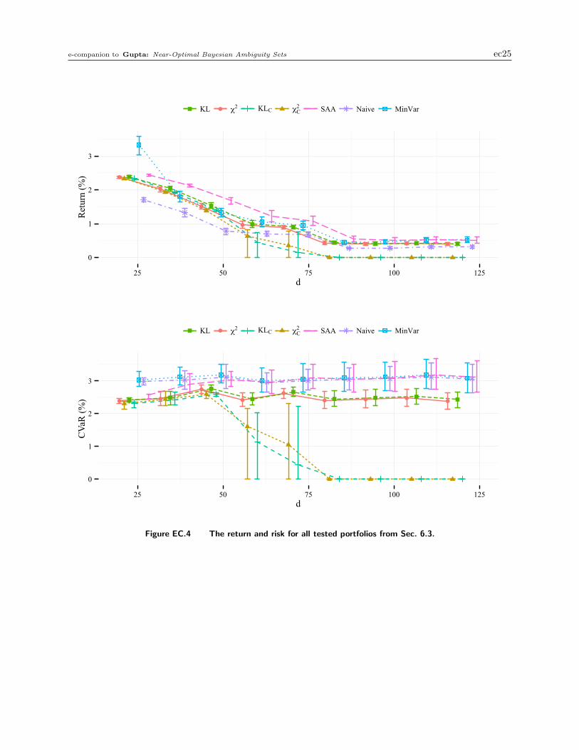
e-companion to Gupta: Near-Optimal Bayesian Ambiguity Sets ec25
●
●
●
● ●
● ● ● ●
0
1
2
3
25 50 75 100 125d
Ret
urn
(%)
●KL χ2 KLC χC2 SAA Naive MinVar
● ●
●
●
●
● ● ●●
0
1
2
3
25 50 75 100 125d
CVa
R (%
)
●KL χ2 KLC χC2 SAA Naive MinVar
Figure EC.4 The return and risk for all tested portfolios from Sec. 6.3.

ec26 e-companion to Gupta: Near-Optimal Bayesian Ambiguity Sets
●
●
●
●●
● ● ● ●
0
1
2
3
25 50 75 100 125d
Ret
urn
(%)
●KL χ2 KLC χC2 SAA Naive MinVar
●●
●
●
●● ● ●
●
0
1
2
3
25 50 75 100 125d
CVa
R (%
)
●KL χ2 KLC χC2 SAA Naive MinVar
Figure EC.5 The return and risk for all tested portfolios from Sec. 6.3 but with N = 700.

e-companion to Gupta: Near-Optimal Bayesian Ambiguity Sets ec27
Table EC.2 Summary statistics of out-of-sample portfolio performance for various randomly generated priors
from Sec. 6.4. The columns 10% and 90% refer the sample quantiles of corresponding statistics.
Return CVaR
Method Strength (%) Avg. 10% 90% Avg. 10% 90%
ChiSq 10 0.90 0.85 0.96 2.65 2.51 2.7925 0.91 0.85 0.97 2.66 2.52 2.8150 0.92 0.86 0.99 2.69 2.54 2.8375 0.92 0.85 0.99 2.71 2.56 2.88100 0.94 0.86 1.02 2.76 2.57 2.96125 0.93 0.85 1.03 2.75 2.57 2.95150 0.94 0.85 1.03 2.78 2.59 2.98
KL 10 0.92 0.87 0.98 2.69 2.55 2.8325 0.93 0.87 0.99 2.70 2.56 2.8550 0.94 0.87 1.01 2.73 2.58 2.8875 0.94 0.86 1.01 2.75 2.59 2.93100 0.96 0.87 1.05 2.81 2.61 3.01125 0.95 0.86 1.06 2.80 2.61 3.01150 0.96 0.86 1.06 2.83 2.62 3.05
1
2
3
2000 2005 2010 2015
Wealth
KL
χ2
KLC
χC2
SAA
Naive
MinVar
Figure EC.6 Realized performance of each portfolio from Sec. 6.5 from Mar. 1998 through Dec. 2014.

ec28 e-companion to Gupta: Near-Optimal Bayesian Ambiguity Sets
0
5
10
2004 2006 2008 2010 2012 2014
Rol
ling
CVa
RKL χ2 KLC χC
2 SAA Naive MinVar
Figure EC.7 Rolling CVaR of each portfolio from Sec. 6.5 using a trailing 72-month window from Mar. 2004
through Dec. 2014.