3 Hyperbolic Geometry in Klein’s Model

3.1 Setup of Klein’s model

The second important model for hyperbolic geometry goes back to Felix Klein. Thereader should recall the basic idea of a model in mathematics, as explained in thepassage General remark about models in mathematics. Again, one uses the Euclideanplane as ambient underlying reality (”background ontology”). We put into the Euclideanplane the open unit disk

D = {(x, y) : x2 + y2 < 1}with the boundary

∂D = {(x, y) : x2 + y2 = 1}The center of D is denoted by O.

Definition 3.1 (Basic elements of Klein’s model). The points ofD are the "points"for Klein’s model. The points of ∂D are called "ideal points" or "endpoints". Theideal points are not points of the hyperbolic plane. Once the hyperbolic distance isintroduced, the points of ∂D turn out to be infinitely far away. Hence we call ∂D the"circle of infinity". The "lines" for Klein’s model are straight chords.

Poincare’s and Klein’s model differ, because lines are represented differently, and—even more importantly—the hyperbolic isometries are given by different types of map-pings. In Poincare’s model, the hyperbolic reflections are realized as inversions by circles.In Klein’s model, the hyperbolic reflections are realized quite differently. Indeed, hyper-bolic reflections are projective mappings, which leave the circle of infinity ∂D invariant.

The developing Klein’s model based on projective geometry is postponed to the sub-section about the projective nature of Klein’s model. I shall now use a rather simple-minded different approach: there exists an isomorphism which is a translation fromPoincare’s to Klein’s model. Because we already know that Poincare’s model is a con-sistent model for hyperbolic geometry, the translation implies that Klein’s model is aconsistent model for hyperbolic geometry, too.

Proposition 3.1 (The mapping from Poincare’s to Klein’s model). The point Pin Poincare’s model is mapped to a point K in Klein’s model by requiring that the rays−→OP =

−−→OK are identical and

(3.1) |OK| = 2 |OP |1 + |OP | 2

The mapping (3.1) keeps the ideal endpoints fixed, and it takes a circular arc l ⊥ ∂Dto the corresponding chord with the same ideal endpoints. Indeed, the mapping (3.1) isa translation of Poincare’s to Klein’s model , since the points and lines of Poincare’smodel, are mapped to points and lines of Klein’s model, preserving incidence.

797

Reason. As shown in the last proposition of the section on Poincare’s model, point K is

the intersection of ray−→OP with the chord between the ideal endpoints of any arc l ⊥ ∂D

through point P . This chord k is a hyperbolic line in Klein’s model. Clearly all pointsof arc l are mapped to points of chord k by the same construction, and hence are allgiven by mapping (3.1).

For the Poincare disk model, it has been very useful to define polar elements outsidethe closed disk D. We shall use polar elements for Klein’s model, too. As a first step,we define and construct the inverse point P ′ of any given point P , in the way explainedin the section about the Euclidean geometry of circles II.

Definition 3.2 (The polar elements for Klein’s model). The polar l⊥ of a line lis the intersection point of the tangents to ∂D at its ideal endpoints.

The Klein polar or projective polar K⊥ of a point K is perpendicular to the ray−−→OK

at the inverse point K ′.

A few clarifying remarks are in place: For both the Poincare and the Klein model,the polar of a line is the intersection point of the tangents to the circle of infinity at theideal ends.

But the mapping from the points to their polar elements are different for the twomodels. For clarification, I use the terms Poincare polar and projective polar. 56 Thedifference occurs because the points are mapped from Poincare’s to Klein’s via theisomorphism (3.1), but the polar elements are the same for both models, hence themappings from points to their polar are different for the two models.

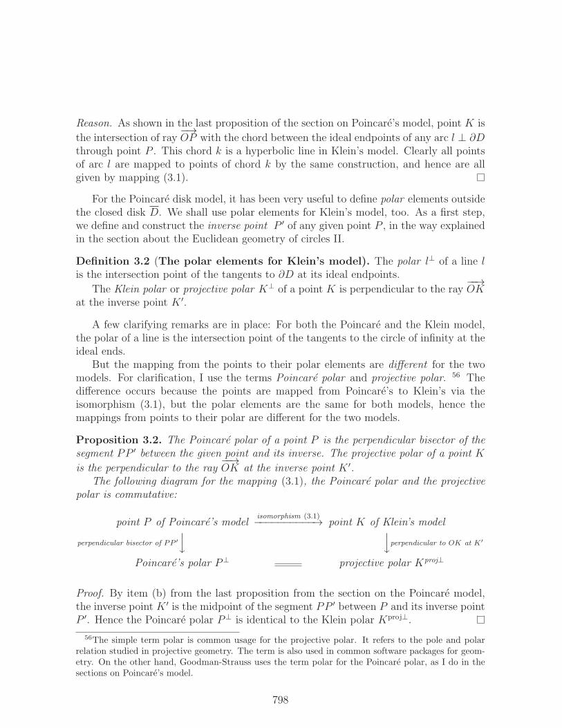
Proposition 3.2. The Poincare polar of a point P is the perpendicular bisector of thesegment PP ′ between the given point and its inverse. The projective polar of a point Kis the perpendicular to the ray

−−→OK at the inverse point K ′.

The following diagram for the mapping (3.1), the Poincare polar and the projectivepolar is commutative:

point P of Poincare’s modelisomorphism (3.1)−−−−−−−−−−→ point K of Klein’s model

perpendicular bisector of PP ′⏐⏐� ⏐⏐�perpendicular to OK at K′

Poincare’s polar P⊥ projective polar Kproj⊥

Proof. By item (b) from the last proposition from the section on the Poincare model,the inverse point K ′ is the midpoint of the segment PP ′ between P and its inverse pointP ′. Hence the Poincare polar P⊥ is identical to the Klein polar Kproj⊥.

56The simple term polar is common usage for the projective polar. It refers to the pole and polarrelation studied in projective geometry. The term is also used in common software packages for geom-etry. On the other hand, Goodman-Strauss uses the term polar for the Poincare polar, as I do in thesections on Poincare’s model.

798

Figure 3.1: A bundle of hyperbolic lines l, l1 through a common point P in Poincare’smodel. They intersect in a common point K in Klein’s model, too. Their polar elements areidentical for both models.

In figure 3.1, Poincare’s elements are drawn in blue, Klein’s elements in brown, andthe polar elements are green. This should make clear the meaning of the commutativediagram in proposition 3.2.

Proposition 3.3. The definitions of the projective polar of points and lines are consis-tent with incidence: A point K lies on a hyperbolic line k if and only if the projectivepolar Kproj⊥ goes through the polar k⊥.

Proof using the development above. As shown in the last proposition in the section aboutPoincare’s model, the point K lies on a chord k if and only if the Poincare point P lieson the arc l ⊥ ∂D with the same endpoints. This happens if and only if the polar l⊥ lieson P⊥. But by proposition 3.2, these polar elements are identical with those of Klein’smodel: l⊥ = k⊥ and P⊥ = Kproj⊥.

Hence, expressing everything in Klein’s model, we conclude that a point K lies on ahyperbolic line k if and only if the polar Kproj⊥ goes through the polar k⊥.

Direct independent proof. Assume that point K lies on line l. We need to check whetherthe polar Kproj⊥ goes through l⊥.

799

Figure 3.2: If line l goes through point K, then the polar l⊥ lies on the polar Kproj⊥.

As drawn in figure 3.1, let L be the foot point of the perpendicular dropped fromcenter O onto line l. The definitions of the polar and the inverse point can easily be

seen to imply l⊥ = L′. Let L′′ be the intersection of ray−→OL and the polar Kproj⊥. This

construction ensures that the polar Kproj⊥ goes point L′′.The triangles �OKL and �OL′′K ′ are equiangular. Hence, by Euclid VI.4, their

sides are proportional to each other:

|OK||OL| =

|OL′′||OK ′|

By definition of the inverse point

|OK| · |OK ′| = 1and hence

|OL| · |OL′′| = 1which shows that L′′ is the inverse point of L. Now L′′ = L′ and L′ = l⊥ implyL′′ = l⊥. Hence the polar Kproj⊥ goes through l⊥, as to be shown. The converse followsas easily.

Before discussing the metric properties and congruence, we need to clarify someterms about the use of any mathematical models, as Klein’s or Poincare’s:

800

Definition 3.3. A theorem or a feature of a figure is part of neutral geometry if andonly if it can be deducted assuming only the axioms of incidence, order, congruence.

The facts of neutral geometry are valid in both Euclidean and hyperbolic geometry—as well as the more exotic non-Archimedean geometries.

Definition 3.4. A feature of a figure drawn inside Klein’s model (as for example anangle, midpoint, altitude or bisector) is called absolute if it is valid both for the under-lying Euclidean plane, on which the model is based, and the hyperbolic geometry insidethe model.

Remark. Here are some features that are absolute, valid both as features of hyperbolicgeometry and in the underlying Euclidean plane: An angle with the center of Klein’sdisk appears as an absolute angle. A right angle of which one side is a diameter appearsabsolute. A perpendicular bisector or an angle bisector which is a diameter appearsabsolute.

Reason. We know that angles are depicted undistorted in Poincare’s model. For thecases mentioned above, the angles are left undistorted by the mapping from Poincare’sto Klein’s model. Hence they are appear absolute in Klein’s model.

Next, we can translate orthogonality. We have shown that in Poincare’s model twohyperbolic lines l and p intersect each other perpendicularly, if and only if the polarl⊥ of one line l and the ideal endpoints P and Q of the other line p lie on a Euclideanline. Since the polar of a line is easily translated, we get the following criterium forperpendicular lines in the Klein model:

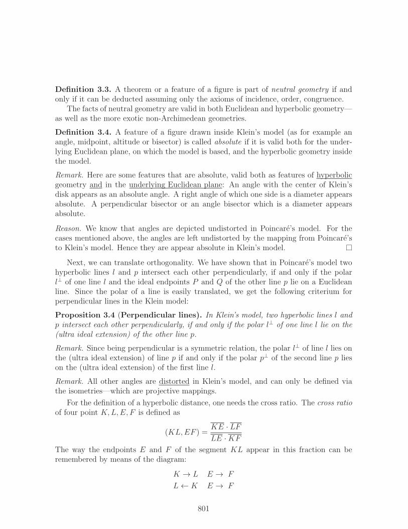
Proposition 3.4 (Perpendicular lines). In Klein’s model, two hyperbolic lines l andp intersect each other perpendicularly, if and only if the polar l⊥ of one line l lie on the(ultra ideal extension) of the other line p.

Remark. Since being perpendicular is a symmetric relation, the polar l⊥ of line l lies onthe (ultra ideal extension) of line p if and only if the polar p⊥ of the second line p lieson the (ultra ideal extension) of the first line l.

Remark. All other angles are distorted in Klein’s model, and can only be defined viathe isometries—which are projective mappings.

For the definition of a hyperbolic distance, one needs the cross ratio. The cross ratioof four point K,L,E, F is defined as

(KL,EF ) =KE · LFLE ·KF

The way the endpoints E and F of the segment KL appear in this fraction can beremembered by means of the diagram:

K → L E → F

L← K E → F

801

Figure 3.3: Two perpendicular lines l and p.

Definition 3.5 (Hyperbolic distance and congruence of segments). Let K,L beany two points. Let the hyperbolic line through K and L denoted by l, and the idealendpoints of this line by E and F . We name those endpoints such that E ∗ L ∗K ∗ F .The hyperbolic distance or simply "distance" of points K and L is defined by

(3.2) s(K,L) =1

2ln(KL,EF ) =

1

2lnKE · LFLE ·KF

As usual, the length of a segment is the distance of its endpoints. Two segments arecalled "congruent" if they have the same length.

3.2 Angle of parallelism

To check that formula (3.2) is the correct translation of the distance function of Poincare’smodel, we use this definition of distance to derive the same formula for the angle of par-allelism as is valid in Poincare’s model.

Proposition 3.5 (The angle of parallelism in Klein’s model). For any point Pand line l, the angle of parallelism π(s) relates the hyperbolic distance s = s(P,Q) from

802

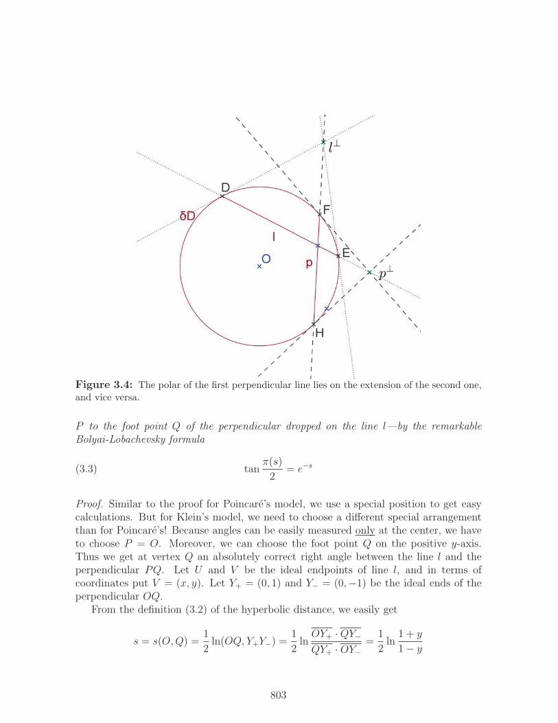
Figure 3.4: The polar of the first perpendicular line lies on the extension of the second one,and vice versa.

P to the foot point Q of the perpendicular dropped on the line l—by the remarkableBolyai-Lobachevsky formula

(3.3) tanπ(s)

2= e−s

Proof. Similar to the proof for Poincare’s model, we use a special position to get easycalculations. But for Klein’s model, we need to choose a different special arrangementthan for Poincare’s! Because angles can be easily measured only at the center, we haveto choose P = O. Moreover, we can choose the foot point Q on the positive y-axis.Thus we get at vertex Q an absolutely correct right angle between the line l and theperpendicular PQ. Let U and V be the ideal endpoints of line l, and in terms ofcoordinates put V = (x, y). Let Y+ = (0, 1) and Y− = (0,−1) be the ideal ends of theperpendicular OQ.

From the definition (3.2) of the hyperbolic distance, we easily get

s = s(O,Q) =1

2ln(OQ, Y+Y−) =

1

2lnOY+ ·QY−QY+ ·OY−

=1

2ln1 + y

1− y

803

Figure 3.5: The angle of parallelism in Klein’s model.

in terms of the cross ratio (OQ, Y+Y−) and the Euclidean distance y = OQ. Applyingthe exponential function yields

(3.4) es =

√1 + y

1− yThe angle of parallelism is defined to be the angle between the perpendicular and theasymptotic parallel. For point O and line QV , the distance point to line is s = |OQ|,and the corresponding angle of parallelism is π(s) = ∠V OQ. Next, we need to gettan π(s)

2. By Euclid III.21, the angle at the circumference is half the angle at the center.

Hence π(OQ)2

= ∠V Y−Q. Now the definition of the tangent function, used for the righttriangle �V QY−, is

tanπ(s)

2=V Q

Y−Q=

x

1 + y

Because V = (x, y) is an ideal endpoint, it lies on the unit circle ∂D. Hence Pythagoras’theorem yields x2 + y2 = 1. One can eliminate x and get

x

1 + y=

√1− y21 + y

=

√(1 + y)(1− y)(1 + y)2

=

√1− y1 + y

804

and hence

(3.5) tanπ(s)

2=

√1− y1 + y

Because of the factor one half in the definition of the hyperbolic distance, everythingfits well! Formulas (3.4) and (3.5) yield

tanπ(s)

2=

√1− y1 + y

= e−s

which is just Bolyai’s formula (3.3) for the angle of parallelism.

As a further benefit of Klein’s model, I shall confirmed Bolyai’s construction of theasymptotic parallel ray.

Construction 3.1 (Bolyai’s Construction of the Asymptotic Parallel Ray).Given is a line l and a point P not on that line. Drop the perpendicular from P ontoline l and let Q be the foot point. Erect the perpendicular onto PQ at point P . One getsa line m parallel to l. Choose a second point R on line l, and drop the perpendicular fromthat point onto m. Let S be the foot point. So far, we have got a Lambert quadrilateral�PQRS. Now one draws a circle of radius QR around the center P . Let B be the

intersection point of that circle with segment RS. Thus one gets a ray−−→PB asymptotically

parallel to the given line l.

Reason. Similar as in proposition 3.5, we use Klein’s model with disk D and put thepoint P = O at the center of the disk. We can put the foot point Q on a verticaldiameter of D.

With this layout, all three right angles of the Lambert quadrilateral �PQRS appearas right angles in Klein’s model. Indeed, PQ is a vertical radius of D and PS is ahorizontal radius of D, and hence the right angles at vertices P,Q and S are absoluteright angles.

Let the line l = QR have ideal ends U and V . Next, we draw the line c = OV .Let V ′ be its second ideal end. The lines RS and c intersect (why?). 57 We call theintersection point B. Thus line c = OB has the ideal endpoints V and V ′.

The following argument refers to the underlying Euclidean geometry (not to thehyperbolic geometry!). In the drawings, I indicate an hyperbolic right angle by a square,but a right angle for the underlying Euclidean geometry gets a doubled arc.

By Thales’ theorem, ∠V ′UV is a right angle for the underlying Euclidean geometry.Hence, again in the underlying Euclidean geometry, the three lines UV ′, QP and RS

57Points R and S lie on different sides of line OV .

805

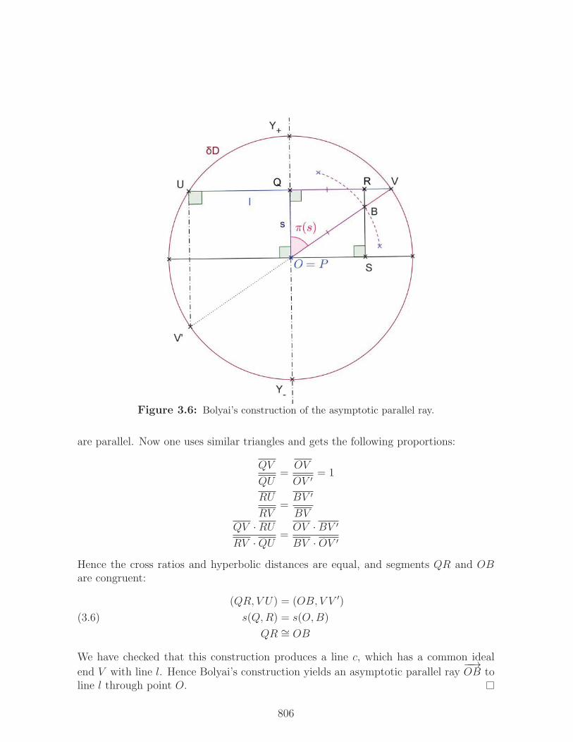
Figure 3.6: Bolyai’s construction of the asymptotic parallel ray.

are parallel. Now one uses similar triangles and gets the following proportions:

QV

QU=OV

OV ′= 1

RU

RV=BV ′

BVQV ·RURV ·QU =

OV · BV ′BV ·OV ′

Hence the cross ratios and hyperbolic distances are equal, and segments QR and OBare congruent:

(3.6)

(QR, V U) = (OB, V V ′)

s(Q,R) = s(O,B)

QR ∼= OB

We have checked that this construction produces a line c, which has a common ideal

end V with line l. Hence Bolyai’s construction yields an asymptotic parallel ray−−→OB to

line l through point O.

806

Because of the congruence (3.6), Bolyai’s construction works inside the hyperbolicplane without using the ideal endpoint V . Indeed, the construction works without needof a model like Klein’s or Poincare’s—and was discovered by Bolyai long before eithermodel was known. The essential step is to draw a circle of radius QR around the centerP . One get is the intersection point B of that circle with segment RS, and finally thelimiting parallel OB.

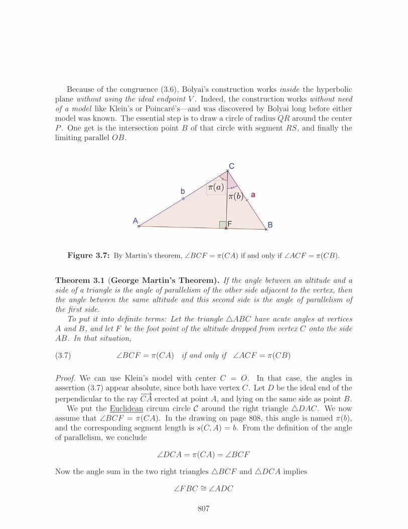
Figure 3.7: By Martin’s theorem, ∠BCF = π(CA) if and only if ∠ACF = π(CB).

Theorem 3.1 (George Martin’s Theorem). If the angle between an altitude and aside of a triangle is the angle of parallelism of the other side adjacent to the vertex, thenthe angle between the same altitude and this second side is the angle of parallelism ofthe first side.To put it into definite terms: Let the triangle �ABC have acute angles at vertices

A and B, and let F be the foot point of the altitude dropped from vertex C onto the sideAB. In that situation,

(3.7) ∠BCF = π(CA) if and only if ∠ACF = π(CB)

Proof. We can use Klein’s model with center C = O. In that case, the angles inassertion (3.7) appear absolute, since both have vertex C. Let D be the ideal end of the

perpendicular to the ray−→CA erected at point A, and lying on the same side as point B.

We put the Euclidean circum circle C around the right triangle �DAC. We nowassume that ∠BCF = π(CA). In the drawing on page 808, this angle is named π(b),and the corresponding segment length is s(C,A) = b. From the definition of the angleof parallelism, we conclude

∠DCA = π(CA) = ∠BCF

Now the angle sum in the two right triangles �BCF and �DCA implies∠FBC ∼= ∠ADC

807

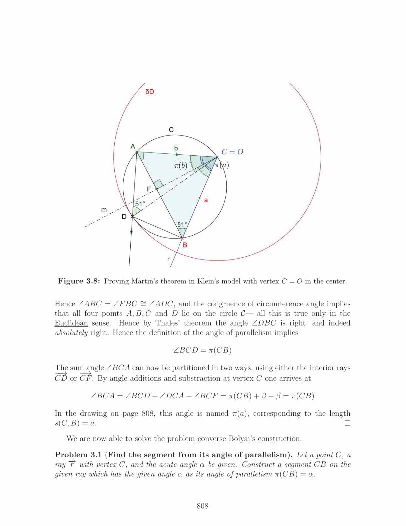
Figure 3.8: Proving Martin’s theorem in Klein’s model with vertex C = O in the center.

Hence ∠ABC = ∠FBC ∼= ∠ADC, and the congruence of circumference angle impliesthat all four points A,B,C and D lie on the circle C— all this is true only in theEuclidean sense. Hence by Thales’ theorem the angle ∠DBC is right, and indeedabsolutely right. Hence the definition of the angle of parallelism implies

∠BCD = π(CB)

The sum angle ∠BCA can now be partitioned in two ways, using either the interior rays−−→CD or

−→CF . By angle additions and substraction at vertex C one arrives at

∠BCA = ∠BCD + ∠DCA− ∠BCF = π(CB) + β − β = π(CB)

In the drawing on page 808, this angle is named π(a), corresponding to the lengths(C,B) = a.

We are now able to solve the problem converse Bolyai’s construction.

Problem 3.1 (Find the segment from its angle of parallelism). Let a point C, aray −→r with vertex C, and the acute angle α be given. Construct a segment CB on thegiven ray which has the given angle α as its angle of parallelism π(CB) = α.

808

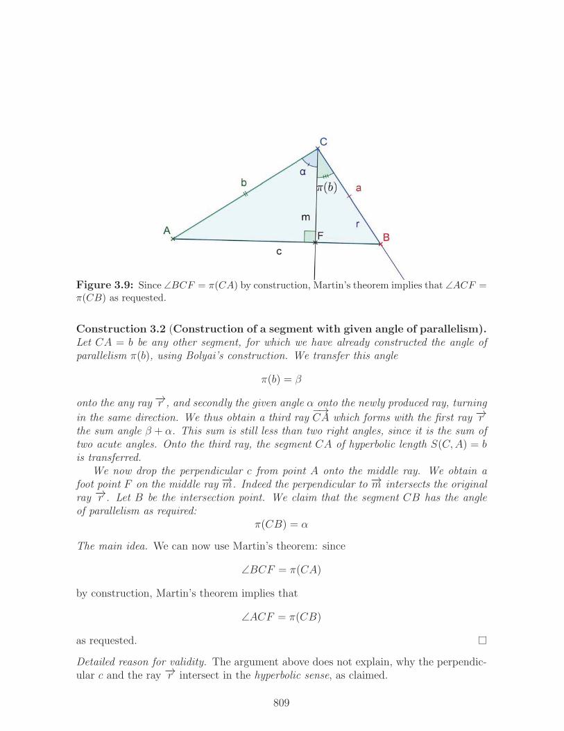
Figure 3.9: Since ∠BCF = π(CA) by construction, Martin’s theorem implies that ∠ACF =π(CB) as requested.

Construction 3.2 (Construction of a segment with given angle of parallelism).Let CA = b be any other segment, for which we have already constructed the angle ofparallelism π(b), using Bolyai’s construction. We transfer this angle

π(b) = β

onto the any ray −→r , and secondly the given angle α onto the newly produced ray, turningin the same direction. We thus obtain a third ray

−→CA which forms with the first ray −→r

the sum angle β + α. This sum is still less than two right angles, since it is the sum oftwo acute angles. Onto the third ray, the segment CA of hyperbolic length S(C,A) = bis transferred.We now drop the perpendicular c from point A onto the middle ray. We obtain a

foot point F on the middle ray −→m. Indeed the perpendicular to −→m intersects the originalray −→r . Let B be the intersection point. We claim that the segment CB has the angleof parallelism as required:

π(CB) = α

The main idea. We can now use Martin’s theorem: since

∠BCF = π(CA)

by construction, Martin’s theorem implies that

∠ACF = π(CB)

as requested.

Detailed reason for validity. The argument above does not explain, why the perpendic-ular c and the ray −→r intersect in the hyperbolic sense, as claimed.

809

We need to repeat the details for a proper justification. We can use Klein’s modelwith center C = O. In that position, the angles α and β constructed above appear abso-lute, because they all have vertex C. Let D ∈ ∂D be the ideal end of the perpendicular

to the ray−→CA at point A, lying on the same side as foot point F . By the definition of

the angle of parallelism,∠DCA = π(CA) = β

In the sense of Euclidean geometry, both ∠ABC = ∠FBC = R−π(CA) and ∠ADC =R − π(CA). The congruence of these angles ∠ADC ∼= ∠ABC implies that the fourpoints A,B,C and D lie on a circle C in the Euclidean sense.

This circle is the Euclidean circum circle of the right triangle �DAC. By theconverse Thales theorem, this circle has diameter CD, which is a radius of Klein’s disk.Hence circle C touches the line of infinity ∂D from inside at the ideal endpoint D. Wecan conclude that point B lies inside Klein’s disk. Thus the perpendicular c and theray −→r intersect in the hyperbolic sense in point B, as claimed.

The remaining details are easy by now: By Thales’ theorem, the angle ∠DBC is aright angle. This is indeed an absolute right angle, because its side BC goes throughthe center of the Klein disk. Hence, by the definition of the angle of parallelism,

π(CB) = ∠DCB = ∠ACB − ∠DCA = α + β − β = α

as to be shown.

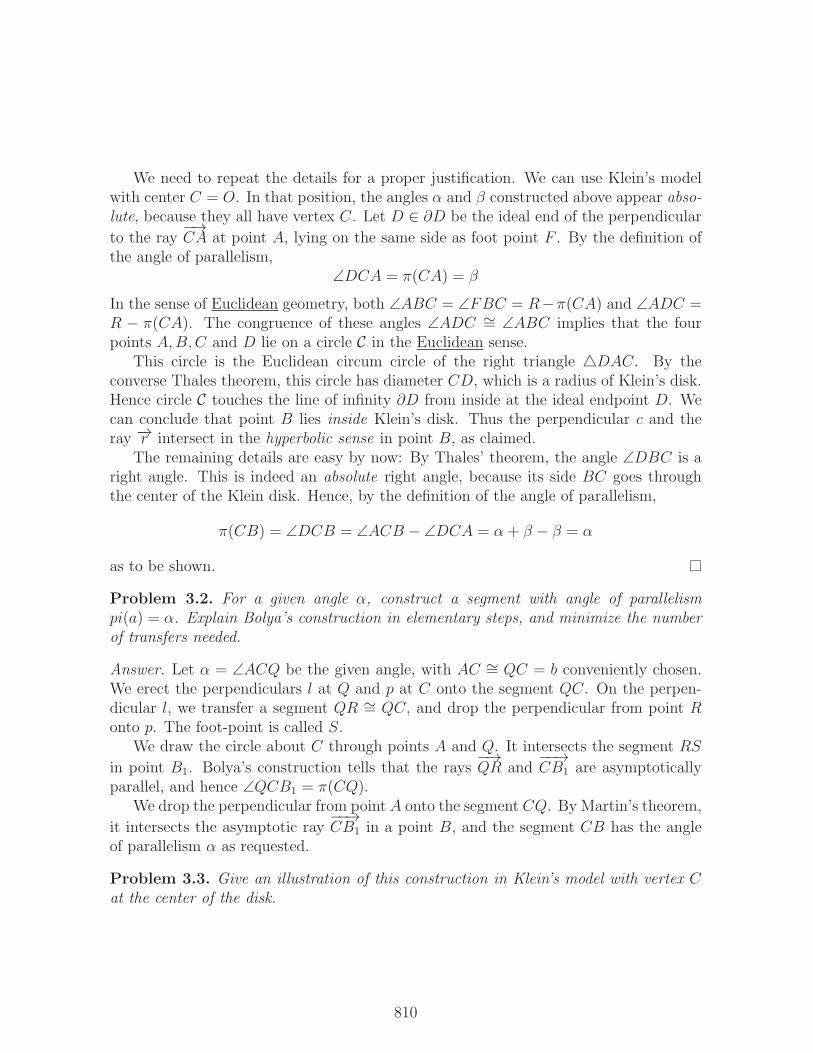
Problem 3.2. For a given angle α, construct a segment with angle of parallelismpi(a) = α. Explain Bolya’s construction in elementary steps, and minimize the numberof transfers needed.

Answer. Let α = ∠ACQ be the given angle, with AC ∼= QC = b conveniently chosen.We erect the perpendiculars l at Q and p at C onto the segment QC. On the perpen-dicular l, we transfer a segment QR ∼= QC, and drop the perpendicular from point Ronto p. The foot-point is called S.

We draw the circle about C through points A and Q. It intersects the segment RS

in point B1. Bolya’s construction tells that the rays−→QR and

−−→CB1 are asymptotically

parallel, and hence ∠QCB1 = π(CQ).We drop the perpendicular from point A onto the segment CQ. By Martin’s theorem,

it intersects the asymptotic ray−−→CB1 in a point B, and the segment CB has the angle

of parallelism α as requested.

Problem 3.3. Give an illustration of this construction in Klein’s model with vertex Cat the center of the disk.

810

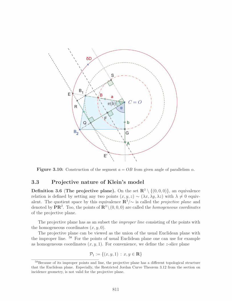
Figure 3.10: Construction of the segment a = OB from given angle of parallelism α.

3.3 Projective nature of Klein’s model

Definition 3.6 (The projective plane). On the set R3 \ {(0, 0, 0)}, an equivalencerelation is defined by setting any two points (x, y, z) ∼ (λx, λy, λz) with λ = 0 equiv-alent. The quotient space by this equivalence R3/∼ is called the projective plane anddenoted by PR2. Too, the points of R3 \(0, 0, 0) are called the homogeneous coordinatesof the projective plane.

The projective plane has as an subset the improper line consisting of the points withthe homogeneous coordinates (x, y, 0).

The projective plane can be viewed as the union of the usual Euclidean plane withthe improper line. 58 For the points of usual Euclidean plane one can use for exampleas homogeneous coordinates (x, y, 1). For convenience, we define the z-slice plane

P1 := {(x, y, 1) : x, y ∈ R}58Because of its improper points and line, the projective plane has a different topological structure

that the Euclidean plane. Especially, the Restricted Jordan Curve Theorem 3.12 from the section onincidence geometry, is not valid for the projective plane.

811

For any nonsingular 3× 3 matrix A, the linear mapping x ∈ R3 → Ax ∈ R3, induces amapping φA : x ∈ PR2 → x′ = Ax ∈ PR2, by means of the homogeneous coordinates.

For the points of the Euclidean plane, this mapping is given by the fractional lineartransformations

(3.8) x′1 =a11x1 + a12x2 + a13a31x1 + a32x2 + a33

and x′2=a21x1 + a22x2 + a23a31x1 + a32x2 + a33

The mapping of the points on the improper line can be rather easily deduced from theseformulas. The details can be left to the reader.

Definition 3.7 (Projective mapping). The extensions of the fractional linear map-pings (3.8) with detA = 0, to the projective plane are called projective mappings.Main Theorem 32. Given are four points x1, x2, x3, x4 ∈ PR2 with no three of themlying on a line. Similarly, there are given any four image points x′1, x

′2, x

′3, x

′4 ∈ PR2.

Once more, it is assumed that no three of them lie on a line. Then there exists exactlyone projective mapping which takes xi to x

′i for i = 1, 2, 3, 4.

Proof. Let x1, x2, x3, x4 ∈ R3 \ {0} be any homogenous coordinates of the four givenpoints xi ∈ PR2. Since any four vectors in R3 are linearly dependent, there existsλ1, λ2, λ3, λ4 ∈ R such that

λ1x1 + λ2x2 + λ3x3 + λ4x4 = 0

Since by assumption no three of the four points xi lie on a line, all four λi = 0 arenonzero. The matrix A = [λ1x1, λ2x2, λ3x3] maps

p1 = (1, 0, 0) → λ1x1 , p2 = (0, 1, 0) → λ2x2 , p3 = (0, 0, 1) → λ3x3 ,

p4 = (1, 1, 1) → −λ4x4 ,

and is nonsingular. The induced projective mapping φA : x ∈ PR2 → x′ = Ax ∈ PR2,takes the points fi → xi for i = 1, 2, 3, 4.

By means of composition A′ ◦ A−1, we find a projective mapping such thatxi ∈ PR2 → x′i ∈ PR2

where the four preimages xi and images x′i can be arbitrarily prescribed.

Main Theorem 33 (Projective invariance of the cross ratio). Let P1, P2, P3, P4

be any four points on a line and Q1, Q2, Q3, Q4 their images by a projective mapping.Then the four points Qi lie on a line, too. The cross ratios (P1P2, P3P4) = (Q1Q2, Q3Q4)are equal.

Definition 3.8. The projective mappings which leave the circle of infinity ∂D invariantare called automorphic collineations.

812

With composition of mappings as group operation, the automorphic collineationsform a group. The following fact shows that it is a rather large group.

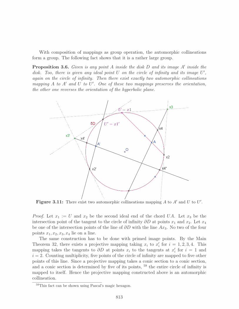
Proposition 3.6. Given is any point A inside the disk D and its image A′ inside thedisk. Too, there is given any ideal point U on the circle of infinity and its image U ′,again on the circle of infinity. Then there exist exactly two automorphic collineationsmapping A to A′ and U to U ′. One of these two mappings preserves the orientation,the other one reverses the orientation of the hyperbolic plane.

Figure 3.11: There exist two automorphic collineations mapping A to A′ and U to U ′.

Proof. Let x1 := U and x2 be the second ideal end of the chord UA. Let x3 be theintersection point of the tangent to the circle of infinity ∂D at points x1 and x2. Let x4be one of the intersection points of the line of ∂D with the line Ax3. No two of the fourpoints x1, x2, x3, x4 lie on a line.

The same construction has to be done with primed image points. By the MainTheorem 32, there exists a projective mapping taking xi to x

′i for i = 1, 2, 3, 4. This

mapping takes the tangents to ∂D at points xi to the tangents at x′i for i = 1 and

i = 2. Counting multiplicity, five points of the circle of infinity are mapped to five otherpoints of this line. Since a projective mapping takes a conic section to a conic section,and a conic section is determined by five of its points, 59 the entire circle of infinity ismapped to itself. Hence the projective mapping constructed above is an automorphiccollineation.

59This fact can be shown using Pascal’s magic hexagon.

813

Because of the arbitrary choice of x′4 among the two intersections of line A′x′3 and

∂D, one gets two solutions. These are the only solutions, because lines are mapped tolines and tangents to ∂D are mapped to tangents to ∂D.

Proposition 3.7. Given any three different ideal points U, V,W on the circle of in-finity and three different images U ′, V ′,W ′, again on the circle of infinity. Then thereexists exactly one automorphic collineation mapping U → U ′, V → V ′,W → W ′. Itdepends on the order of the given points, whether the mapping preserves or reverses theorientation of the hyperbolic plane.

Answer (Proof of Proposition 3.7). Let x1 be the intersection point of the tangents at Uand V to ∂D, and x′1 be the intersection point of the tangents at U

′ and V ′ to ∂D. Of thefour points x1, U, V,W no three lie on a line, and similarly for the points x′1, U

′, V ′,W ′

By the Main Theorem 32, there exists exactly one projective mapping taking x1 → x′1and U → U ′, V → V ′,W → W ′. This mapping takes the tangents to ∂D at points Uand V to the tangents at U ′ and V ′. Counting multiplicity, five points of the circle ofinfinity are mapped to five other points of this line. Since a projective mapping takes aconic section to a conic section, and a conic section is determined by five of its points,the entire circle of infinity is mapped to itself. Hence the projective mapping constructedabove is an automorphic collineation.

On the other hand, the obtained mapping is unique, since any automorphic collineationwith the required property necessarily maps x1 to x

′1.

Figure 3.12: An automorphic collineation that transports points along horocycles.

814

Proposition 3.8. Given any ideal point U on the circle of infinity and any two differentpoints A and A′ on the tangent to the circle ∂D at point U . Then there exists exactlyone automorphic collineation which keeps U fixed, map A to A′ and has no other fixedpoint. This mapping preserves the orientation of the hyperbolic plane.

Proof of Proposition 3.8. Let X and X ′ be the touching points of the tangents frompoints A and A′ to ∂D. We let Z ′ be the intersection point of these tangents and drawthe line b = UZ ′. Let Y ′ be the second end of line b, let Y be the second end of lineAY ′.

Of the four points A,X, Y, U nor of the four points A′, X ′, Y ′, U no three lie on aline. By the Main Theorem 32, there exists exactly one projective mapping taking

A → A′, X → X ′, Y → Y ′, and leaving point U → U

fixed. This mapping takes the tangents to ∂D at points U and X to the tangents at Uand X ′ since A is mapped to A′. Furthermore point Y ∈ ∂D is mapped to Y ′ ∈ ∂D.Counting multiplicity, five points of the circle of infinity are mapped to five other pointsof this circle. Hence the prescribed mapping is an automorphic collineation.

On the other hand, the obtained mapping is unique, since any automorphic collineationwith the required property necessarily maps A → A′, X → X ′, Y → Y ′ and leaving pointU → U fixed. It is left to the reader to check that X, Y, U and X ′, Y ′, U define the sameorientation of the circle ∂D.

Problem 3.4. Convince yourself that the automorphic collineation constructed above isthe composition Rb ◦Ra of the two reflections across lines a and b.Solution. The reflection Ra takes X → X, Y → Y ′, leaving point U → U fixed.The reflection Rb takes X → X ′, Y ′ → Y ′, leaving point U → U fixed. Hence thecomposition Rb ◦Ra takes

X → X ′, Y → Y ′, leaving point U → U

fixed. Since it is an automorphic collineation and preserves the orientation, it is uniquelyspecified by this property. Since the given mapping S is an orientation preservingautomorphic collineation with the same property, we conclude S = Rb ◦Ra.

The development of Klein’s model is based on the fact:

Main Theorem 34. The automorphic collineations are the isometries of the hyperbolicplane. They leave the hyperbolic distances and angles invariant.

Proof. The invariance of the distances is an easy consequence of the projective invarianceof the cross ratio. The hyperbolic distance any two points K and L is defined by

(3.9) s(K,L) =1

2ln(KL,EF ) =

1

2lnKE · LFLE ·KF

815

where E and F are the ideal endpoints of the line KL, ordered such that E ∗L ∗K ∗F .Any automorphic collineation maps these four points to points E ′, L′, K ′, F ′, lying

again on one line, and E ′ and F ′ lying on the circle of infinity ∂D. Hence the latter twopoints are the ideal ends of the image line K ′L′ and have the hyperbolic distance

(3.10) s(K ′, L′) =1

2ln(K ′L′, E ′F ′) =

1

2lnK ′E ′ · L′F ′L′E ′ ·K ′F ′

Hence the invariance of the cross ratio by projective mappings implies

KE · LFLE ·KF =

K ′E ′ · L′F ′L′E ′ ·K ′F ′

and hence s(K,L) = s(K ′, L′), as to be shown.

The invariance of the angles allows for measurement of angles. To this end, onemaps the given angle by an automorphic collineation, taking its vertex A to the centerO. Because the image angle has its vertex at the center, it appears as an absolute angleand can be measured by the geometry of the Euclidean plane.

Secondly the construction used in the proof of proposition 3.6 confirms once morethe criterium for right angles given in proposition 3.4.

Our next goal is the construction of a hyperbolic reflection. It turns out that thekey figure is the ideal quadrilateral.

Proposition 3.9 (An ideal quadrilateral produces five right angles). Let theideal quadrilateral �ABCD have diagonals intersecting at P , and drop perpendicularl from point P onto side AB. This perpendicular l is perpendicular to both oppositesides AB and CD. Next we erect the perpendicular p onto l at point P . This secondperpendicular p is perpendicular to the other two opposite sides BC and DA.Furthermore, the three lines AB, CD and p meet in one ultra ideal point, and the

three lines BC, DA and l meet in another one.

Proof. There exists an automorphic collineation that maps the point P to the centerP ′ = O.

Hence the special position with the intersection of the diagonals at the center of thedisk can be achieved by means of an automorphic collineation, which is an isometry ofthe hyperbolic plane.

But in that special position, the diagonals and the lines l and p all intersect at thecenter O. Thales’ theorem now implies that the ideal quadrilateral �ABCD appearsas a rectangle. The five right angles appear as absolute right angles, valid both in theunderlying Euclidean plane and in hyperbolic geometry.

Reason via the Poincare model. Put the figure into the Poincare model, and use thespecial position with the intersection of the diagonals at the center of the disk. As

816

Figure 3.13: An ideal quadrilateral produces five right angles.

shown in the section on the Poincare model, this special position with P = O can beachieved by means of hyperbolic reflections.

But in that special position, the diagonals and the lines l and p are absolute straightlines, and the ideal quadrilateral �ABCD appears as a rectangle. The five right anglesare immediate to confirm.

We now use the ideal quadrilateral for the construction of a hyperbolic reflection.

Construction 3.3 (Hyperbolic reflection of a point by a given line). Given is areflection line l and a point K not on line l. We want to construct the reflective imageof K ′ of K by the line l.Choose any parallel to l with ideal ends B and C, and get the polar BC⊥ as inter-

section point of the tangents at B and C to the circle of infinity ∂D. The line p throughthe points K and BC⊥ is the perpendicular dropped from K onto line l. The foot pointP is the intersection of lines p and l.Finally, to get the reflective image, we draw the line CP with the second end A,

and BP with the second end D, thus producing an ideal quadrilateral �ABCD. Thereflection point K ′ is the intersection of side AD with the perpendicular p.

Remark. The four points K,P , the polar BC⊥, and the intersection of lines AB andCD lie all on the perpendicular p. This property should be used to achieved betteraccuracy.

817

Figure 3.14: Construction of the reflective image K ′ for a given point K and reflection linel.

Construction 3.4 (True hyperbolic angle). Given is a hyperbolic angle ∠OKF .We draw the ends E and F of the line EF and its polar C = EF⊥. The circle aroundC through the ends E and F intersects the segment OK in point P . We draw segmentsEB and FA through point P and obtain the ends A and B. These points are actuallythe endpoints of a diameter. The true hyperbolic angle is ω = ∠KOA.

Proposition 3.10 (Distortion of angles). The measure of the hyperbolic angle ∠OKFcan be obtained by the construction from the figure on page 819 by a reflection across thepoint P . One obtains the true hyperbolic angle ω = ∠KOA with vertex at the center.By the formula

(3.11) tanω = tanα√1− r2

the true angle ω is calculated from the apparent angle α.

Justification of the construction. The mapping from Poincare’s to Klein’s model as ex-plained in proposition 3.1 gives

(3.1) |OK| = 2 |OP |1 + |OP | 2

818

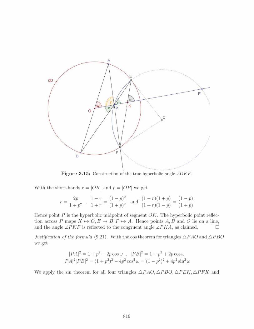
Figure 3.15: Construction of the true hyperbolic angle ∠OKF .

With the short-hands r = |OK| and p = |OP | we get

r =2p

1 + p2,1− r1 + r

=(1− p)2(1 + p)2

and(1− r)(1 + p)(1 + r)(1− p) =

(1− p)(1 + p)

Hence point P is the hyperbolic midpoint of segment OK. The hyperbolic point reflec-tion across P maps K → O,E → B,F → A. Hence points A,B and O lie on a line,and the angle ∠PKF is reflected to the congruent angle ∠PKA, as claimed.

Justification of the formula (9.21). With the cos theorem for triangles�PAO and�PBOwe get

|PA|2 = 1 + p2 − 2p cosω , |PB|2 = 1 + p2 + 2p cosω|PA|2|PB|2 = (1 + p2)2 − 4p2 cos2 ω = (1− p2)2 + 4p2 sin2 ω

We apply the sin theorem for all four triangles �PAO,�PBO,�PEK,�PFK and

819

get

sin2 ω

|PA||PB||PE||PF |sin2 α

=sin x sin y

|OA||OB||KE||KF |sin x sin y

sin2 ω

sin2 α=|PA||PB||PE||PF | |KE||KF | = |PA|

2|PB|2 |KE||KF ||PA||PB||PE||PF |

=[(1− p2)2 + 4p2 sin2 ω] (1− r)(1 + r)

(1− p)2(1 + p)2

Reminding

r =2p

1 + p2, r2 =

4p2

(1 + p2)2, 1− r2 = (1− p2)2

(1 + p2)2,

r2

1− r2 =4p2

(1− p2)2

we get

sin2 ω

sin2 α=

[1 +

(2p

1− p2)2

sin2 ω

](1− r2) = 1− r2 + r2 sin2 ω

sin2 ω =(1− r2) sin2 α1− r2 sin2 α

cos2 ω =1− sin2 α1− r2 sin2 α

tan2 ω = (1− r2) tan2 αMoreover, we see that the angle ω is acute if and only if the angle α is acute, ω isright if and only if α is right, and ω is obtuse if and only if α is obtuse. Hence we getformula (9.21) with the positive square root.

3.4 Engel’s Theorem

In this paragraph, we state and prove Engel’s theorem. This theorem constructs abijective correspondence between right triangles and Lambert quadrilaterals. Klein’smodel is convenient for the proof, which uses a refinement of Bolyai’s construction.

Recall that quadrilaterals with three right angles are called Lambert quadrilaterals.Right triangles and Lambert quadrilaterals both have five basic pieces (angles or sides),and can be constructed once any two of them are given.

Proposition 3.11 (Transfer of a segment on its line). Let E and F be the idealendpoints of line c. We put any two ideal points A,B on one of the two arcs from E toF , and two more points V,W on the other arc on ∂D from E to F . Let P2P3 and Q2Q3

be the segments on line l cut out by the angles ∠V AW and ∠V BW , respectively.The two segments P2P3 and Q2Q3 are hyperbolically congruent.

820

Figure 3.16: Transfer of a segment along its line.

Proof. We need these two basic facts:

(Invariance of the cross ratio for central projections). Given are any two linesacross a bundle of four rays with common vertex. Let P1, P2, P3, P4 and Q1, Q2, Q3, Q4

be the intersection points of the rays with the two lines across the bundle. Then the crossratios (P1P2, P3P4) = (Q1Q2, Q3Q4) are equal. The same statement holds for two linesintersecting two congruent ray bundles.

(Euclid’s III.21). Two angles from points of a circle subtending the same arc are con-gruent.

By Euclid III.21, the two ray bundles−−−−−−−−−→A(E, V,W, F ) and

−−−−−−−−−→B(E, V,W, F ) are congruent.

The two ray bundles intersect line EF in the four points E,P2, P3, F and E,Q2, Q3, F ,respectively. Now we use fact 1 with E = P1 = Q1 and F = P4 = Q4 and get

(P2P3, EF ) = (Q2Q3, EF ) and s(P2, P3) = s(Q2, Q3)

as to be shown.

For s given, one defines s∗ to be the hyperbolic length for which π(s) + π(s∗) = 90◦.The pieces of �ABC are denoted in Euler’s standard fashion.

821

Proposition 3.12 (Engel’s Theorem). There is a bijective (one-to-one and onto)correspondence between right triangles and Lambert quadrilaterals �PQRS. The Lam-bert quadrilateral �PQRS and the right triangle �ABC are matched by putting one legof the Lambert quadrilateral onto one leg of the right triangle, and one of the outer rightangles of the Lambert quadrilateral onto the right angle of the triangle. Thus A = Pand C = S. The correspondence is established by requiring (3.13) and any one of theother four statements (3.12),(3.14),(3.15) or (3.16).In that way, the five pieces of the triangle and of the Lambert quadrilateral are match-

ing as follows:

a := BC has angle of parallelism π(a) = ∠QRS(3.12)

b := AC = PS(3.13)

c := AB = QR(3.14)

α := ∠BAC = π(l∗) with l = PQ(3.15)

β := ∠CBA = π(m) with m = RS(3.16)

Figure 3.17: The correspondence of a Lambert quadrilateral and a right triangle.

Proof. We use Klein’s disk model with disk D and choose as center O = A = P . Thebijective correspondence of �ABC and �PQRS is given by requiring that

(i) A = P and C = S.

(ii) vertex B lies on the ray−→SR.

(iii) Hypothenuse AB and quadrilateral side QR have a common ideal endpoint V .

In the figure on page 806 about Bolyai’s construction of the asymptotic parallel ray, onecan see at once that requirements (i)(ii)(iii) define a bijection between right triangles and

822

Lambert quadrilaterals. For this correspondence, claim (3.13) is obvious. Claim (3.14)and (3.15) both follow from Bolyai’s construction.

Reason of claim (3.15). Indeed point P and line UV have the angle of parallelism

∠V PQ, as angle between the perpendicular PQ and the asymptotic parallel ray−→PV .

Because ∠V AQ is the complementary angle of α = ∠CAB, one gets π(PQ) = 90◦ − αand hence α = π(s(P,Q)∗). This confirms claim (3.15).

Reason of claim (3.12). As shown in figure 3.4, we draw line V ′S and let W be itssecond ideal endpoint. Draw line US and let X be its second ideal endpoint.

The lines RS and PS are perpendicular, and intersect in S. The ideal quadrilateral�V ′UWX has its diagonals intersecting in S. Its side UV ′ is perpendicular to PS.Hence by proposition 3.9, the opposite side WX is perpendicular to PS, too. Fur-thermore, the other two opposite sides UW and V ′X are perpendicular to RS. Thusthe quadrilateral �V ′UWX, its diagonals, and the two perpendicular lines RS and PSproduce the English flag and five right angles, as shown in figure 3.4.

Now we complete the proof of claim (3.12): Let H be the intersection point of thetwo perpendicular lines UW and RS. It can happen that H lies inside the segment SB,or inside the segment BR, or H = B. The figure 3.4 shows the case that H lies insidethe segment BR.

Let E and F be ideal endpoints of line RS = EF . As explained in proposition 3.11

about the transfer of a segment on its line, the two ray bundles−−−−−−−−−→U(E, V,W, F ) and−−−−−−−−−−→

V ′(E, V,W, F ) are congruent. Hence the two segments cut out on line EF are congruent:

(3.17) (HR,EF ) = (SB,EF ) and s(H,R) = s(S,B) = a

The angle of parallelism of segment RH is ∠URH, because it is the angle betweenthe asymptotic parallel ray

−→RU and the perpendicular RH, for point R and line UW .

Hence π(RH) = ∠URH. Combined with (3.17), we conclude Hence π(a) = π(RH) =∠URH = ∠QRS as claimed in (3.12).

823

Figure 3.18: Find the English flag.

Reason of claim (3.16). This is done in the same manner we just have proved (3.12).This time, we use line US and let X be its second ideal endpoint. As shown above, thetwo segments UW and V ′X are both perpendicular to RS. Let G be the intersectionpoint of the perpendicular lines V ′X and SR.

Again by Euclid III.21, the two ray bundles−−−−−−−−−→U(E, V,X, F ) and

−−−−−−−−−−→V ′(E, V,X, F ) are

congruent. The two ray bundles intersect line EF in the four points E,R, S, F andE,B,G, F , respectively. Hence proposition 3.11 implies

(3.18) (RS,EF ) = (BG,EF ) and s(R, S) = s(B,G) = m

Referring to point B and line V ′X, we see that the angle of parallelism of segment BG

is ∠V ′BG, because it is the angle between the asymptotic parallel ray−−→BV ′ and the

perpendicular BG. Hence π(BG) = ∠V ′BG. Combining with (3.18), we conclude thatπ(m) = π(RS) = π(BG) = ∠V ′BG = ∠ABC = β, as claimed in (3.16).

3.5 The Hjelmslev quadrilateral

Theorem 3.2. Hjelmslev’s theorem 10.2 about the quadrilateral with right angles at twoopposite vertices holds in hyperbolic and neutral geometry, too.

824

Figure 3.19: Proof of claim (3.12): a has angle of parallelism π(a) = ∠URH.

Problem 3.5. Prove the angle congruence of Hjelmslev’s Theorem in hyperbolic geom-etry. Assume that the Euclidean theorem has already been shown. Use Klein’s model,and put into the center of the disk the vertex of the pairs of angles that you want tocompare.

Proof of the angle congruence in hyperbolic geometry. I use Klein’s model with the ver-tex B put into the center of the disk. Because angles at the center of the disk areabsolute (not distorted), it suffices to compare the Euclidean angles at B. The right an-gles of the Hjelmslev quadrilateral are absolute right angles, too, since one side of themis a diameter of the Klein disk. Hence the hyperbolic Hjelmslev quadrilateral appearsin Klein’s model as a Euclidean Hjelmslev quadrilateral, too.

Now we can use the Euclidean version of the theorem, and conclude Euclidean con-gruence of the angles β := ∠ABD and β′ = ∠GBC. Because angles at the center of thedisk are not distorted, the Euclidean congruence implies the hyperbolic congruence.

Problem 3.6 (Open problem). Prove the segment congruence of Hjelmslev’s Theoremin hyperbolic geometry. Assume that the Euclidean theorem has already been shown anduse Klein’s model.

825

Figure 3.20: Proof of claim (3.16): m = RS has angle of parallelism π(m) = ∠V ′BG.

Figure 3.21: The angle congruence of Hjelmslev holds in hyperbolic geometry, too.

826