3 housing prices and homicide rate - pàgines de la...
TRANSCRIPT
1
Homicide rate and Housing Prices in Cali-Colombia
By Andres Dominguez and Josep Lluis Raymond
Summary - Latin America dominates list of world’s most violent cities in the world. In 2015 Cali (Colombia) registered 65 homicides per 100,000 people in a ranking headed by Caracas (Venezuela) with 120. However, the crime rates are not homogeneously distributed within an urban area and the literature points out that the local response to crime will be observed in the housing market. The objective of the paper is to estimate the relationship between housing prices and homicide rates in Cali. We found that a 10% increase of the homicide rate is related with a decreasing between 2% and 2.5% in housing prices.
JEL-code – R10
Keywords – housing prices,

2
1. Introduction
High crime rates represent a significant welfare loss, reducing expected lifespan
and increasing uncertainty about the future (Soares, 2010). Furthermore, it is
important the quantity of money assigned to maintain justice and prison systems.
According to CCSP-JP,1 in 2015 Latin America dominates list of world’s most
violent cities. Figure 1 shows 50 worst cities with population higher than 300,000
people. The horizontal axis represents the homicide rate per 100,000 people, while
the size of the circle represents the number of homicides. The ranking is headed by
Caracas (Venezuela), San Pedro Sula (Honduras) and San Salvador (El Salvador).
There are two Colombian cities with high homicide rate: Palmira and Cali. The
former is an intermediate city of 1.5 million inhabitants, and Cali is the third city in
terms of population in Colombia (2.3 million).
There is an association between city size and crime (Glaeser and Sacerdote,
1999), furthermore, the crime rates are not homogeneously distributed within an
urban area and this characteristic has a strong association with the neighbourhood
quality. In response to crime risk, residents generally have two options: they can
vote for anti-crime policies or vote with their feet. When individuals exercise the
latter option, local response to crime will be observed in the housing market
(Gibbons, 2004; Buonanno, et al., 2012). Indeed, the fear of crime through its
indirect effects on housing prices may also hinder local regeneration and cause a
downward spiral in neighbourhood quality (Gibbons, 2004).
1 Council for Public Security and Criminal Justice (CCSP-JP by its Spanish acronym).

3
Figure 1-Homicides per 100,000 people.
Source: The Economist (2016).
There is evidence on the relationship between urban crime and housing prices
for European and North American cities. Soares (2010) points out that death due
to violence is 200 percent more common in Latin America than in North America
and 450 percent more common than in Western Europe. The objective of this
paper is evaluating the relationship between homicide rates and housing prices in
Cali. We use cadastral information of housing prices of 2012 and the average
homicide rates of the period 2000-2010 at neighbourhood level.
The analysis is performed using two estimation strategies. In the first we
estimate a model where the dependent variable is housing prices and one of the
explanation variables is the homicide rate: we found that a 10% increase of the
homicide rate is related with a 2.4% decrease in housing prices. In the second
strategy we estimate a two stage model: in one stage we estimate the hedonic price
at neighbourhood level and next we estimate a regression to test if the homicide
rate has a negative relationship with the estimated hedonic price. We found that, in
average, a 10% increase of the homicide rate is related with a decreasing between
1.4% and 2.7% in housing prices.
Additionally we discuss a methodological issue: when the statistical information
is clustered (e.g. classrooms, neighbourhoods, economic sectors) the literature
recommends to estimate models using cluster standard errors. Nevertheless, there
are some potential harmful consequences on the estimated standard errors
derived from forming false clusters. In this paper we present a simulation exercise
to show the magnitude and the direction of the bias in the standard errors
estimation.

4
The remainder of the paper is organized as follows: section 2 relates the paper
to the existing literature, section 3 describes data and provides the estimation
results, and section 4 concludes.
2. Literature Review
Fear of crime has a powerful influence on perceptions of area deprivation and may
discourage home-buyers, inhibit local regeneration and catalyse a downward
spiral in neighbourhood status (Gibbons, 2004). The literature has tried to
measure the effect of crime on housing prices using two main methodologies:
The contingent valuation tries to estimate the value of a god that is not
transacted in a market. The strategy is to ask how much people would be
willing to pay for it. For example, in Cohen et al. (2004), respondents
were asked if they would be willing to vote for a proposal requiring each
household in their community to pay a certain amount to be used to
prevent one in ten crimes in their community. Meanwhile, in Atkinson et
al. (2005), respondents were told the characteristics of a type of crime
and the current risk of victimization, and then asked to express their
willingness to pay to reduce the chance of being a victim of this offence
by 50 percent over the next 12 months.
In the hedonic models (Rosen, 1974) a house may derive its value from
the quality of its physical characteristics (e.g. living space, number of
bedrooms, garage, amenities), and also from its location. Furthermore,
the level of crime and violence in the surrounding area may be an
additional attributes of the property, and individuals may be willing to
pay more to live in an area with lower levels of crime. Then, an estimate
of how much the attribute lower-level-of-crime is worth in the housing
price provides an estimation of the cost of crime.
Ask individuals how they would react in a certain situation are not real
decision-making situations. Consequently, economists have long been sceptical of

5
information extracted from stated preferences, rather than revealed ones (Carson
et al., 2001; Levitt and List, 2007). This is the reason because hedonic price models
have been most used to estimate the relationship between crime and housing
prices. Hedonic models rely on preferences revealed by market behaviour, by
analyzing the actual amount that people pay to avoid living in high crime areas.
Some literature that uses this methodology found a negative and significant
relationship between crime and housing prices: For Rochester, New York, one
standard deviation increase in the crime rate caused a reduction in the price of a
house of 3% (Thaler, 1976) - the measures of crime used by the author are: total
offences, property crimes, crimes against persons, and property crimes committed
in or around homes -. Hellman and Naroff (1979) obtain an elasticity of property
value with respect to crime equal to -0.63 for Boston. For Jacksonville, Florida,
Lynch and Rasmussen (2001) found an elasticity of -0.05 for violent crimes.
Meanwhile, for Atlanta, Bowes and Ihlanfeldt (2001) argue that crime may be
higher in train station areas; moreover, train stations may cause more crime in
high that in low-income neighbourhoods. Authors found that an additional crime
per-acre per-year decreases housing prices by around 3%. Besley and Mueller
(2012) present evidence that supports the assumption that housing prices depend
on the level and persistence of historical crime rates. Authors argue that houses
are assets whose prices reflect the present and future expected attractiveness of
living in an area. They use information for 11 regions of Northern Ireland to
evaluate the increased housing prices in response to a reduction in killing.
Estimating a Markov switching model authors predict that peace in Northern
Ireland leads to an increase in housing prices of between 1.3 percent and 3.5
percent (the result is heterogeneous across regions).
6
Table 1-Literature review Author Place and time Results Studies that do not instrument for crime Thaler (1978) Rochester, New York (1971). One standard deviation increase in
the crime rate caused a reduction in the price of a house of 3%.
Hellman and Naroff (1979)
Boston (1976). They report a negative elasticity of property value with respect to total crime (-0.63).
Lynch and Rasmussen (2001)
Jacksonville, Florida. They found an elasticity of -0.05 for violent crimes.
Bowes and Ihlanfeldt (2001)
Atlanta (1991-1994). An additional crime per acre per year in a given census tract has the effect of reducing house prices by around 3%.
Shapiro and Hassett (2012)
Seattle, Milwaukee, Huston, Dallas, Boston, Philadelphia, Chicago and Jacksonville.
10% reduction in homicides would lead to a 0.83% increase in housing values the following year
Besley and Mueller (2011)
11 regions of Northern Ireland (1984-2009).
Property prices depend on the level and persistence of historical crime rates.
Frischtak and Mandel (2012)
Rio de Janeiro. Homicides dropped 10% to 25% and robberies 10% to 20%, while the selling price of the properties increased between 5% and 10%, and was proportionally higher in low-income neighbourhoods
Studies that do instrument for crime Instruments Rizzo (1979) Chicago (1970). The estimated elasticity of crime
respect prices is -0.23. Gibbons (2004) London (2001). Crimes on non-
residential properties; Spatial lags of the crime density; Distance to the nearest alcohol licensed premises.
A one-tenth standard deviation increase in the recorded density of incidents of criminal damage has a capitalized cost of just under 1% of property values
Tita, Petras and Greenbaum (2006)
Columbus, Ohio (1995-1998).
Homicide rate. Negative significant relationship between prices and violent crimes.
Ceccato and Wilhelmsson (2011)
Stockholm (2008). Murders as an instrument for crime.
If total crime increases by 1 per cent, apartment prices are expected to fall by 0.04 per cent.
Buonanno et al. (2013) Barcelona (2004-2006).
Victimization rate 20 years ago; Share of youth aged between 15 and 24.
One standard deviation increase in perceived security is associated with a 0.57% increase in the valuation of districts.
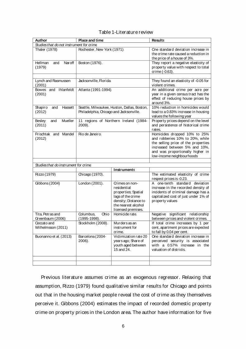
Previous literature assumes crime as an exogenous regressor. Relaxing that
assumption, Rizzo (1979) found qualitative similar results for Chicago and points
out that in the housing market people reveal the cost of crime as they themselves
perceive it. Gibbons (2004) estimates the impact of recorded domestic property
crime on property prices in the London area. The author have information for five

7
types of crime: burglary in a dwelling, burglary in other buildings, criminal damage
to a dwelling, criminal damage to other buildings, and theft from shops. As a result,
a one-tenth standard deviation increase in the recorded density of incidents of
criminal damage has a capitalized cost of just under 1% of property values. This
means that incoming residents perceive criminal damage as a deteriorating
neighbourhood. The difference with previous papers is that the author pays
attention to identification issues and deals with the endogeneity problem using
instrumental variables. Ceccato and Wilhelmsson (2011) analise the relationship
between apartment prices and different measures of crime in Stockholm. Authors
found that when total crime increases in 1%, apartment prices are expected to fall
by 0.04%. Buonanno et al. (2013), for Barcelona, found that one standard deviation
increase in perceived security is associated with a 0.57% increase in the valuation
of districts (authors deal with endogeneity using instrumental variables).
Although compare results is somewhat arbitrary because the differences in the
types of crimes, there is evidence of a negative relationship between crime and
housing prices. This means that high crime rates deter new residents and motivate
those who can to move out to lower-crime rate neighbourhoods (Gibbons, 2004).
3. Data and Results
Cadastral information in Colombia is one of the oldest and largest in Latin America,
nevertheless is limited in order to formulate politics (DAHM, 2012). We use the
cadastral housing prices of 2012 in order to estimate the relationship with
homicide rates at neighbourhood level. Homicide rate is defined as the number of
homicides committed in a year per 100,000 people, excluding homicides
committed as a result of the armed conflict.
Table 2 summarises the key variables in the housing price and homicide data.
The mean of log of housing prices is 17.16 with a standard deviation of 1.21
(Figure 1 shows the distribution this variable); the homicide rate that we use is the
average of ten years (2000-2010) at neighbourhood level, this variable has a mean
of 104 with a standard deviation equal to 155. Firs map on the Figure 2 shows the

8
average housing prices per square meter in Colombian Pesos and second map
shows the homicide rates at neighbourhood level. Our hypothesis is that persistent
cases of homicide will be capitalized in housing prices. The urban area is divided in
338 neighbourhoods: the average size of a neighbourhood is 360 square meters;
the average distance between the Central Business District (CBD) and the centroid
of a neighbourhood is 4.76 kilometres; and the average distance from the centroid
of a neighbourhood to the closer main road is 0.41 kilometres.
Table 2- Summary statistics Mean Std. Dev. Minimum Maximum ln(Housing price) 17.16 1.21 10.99 25.20 Homicide rate 104 155 0 1628 Area (푘푚 ) 0.36 0.50 0.02 7.84 Distance to CBD (푘푚) 4.76 2.12 0 9.78 Distance to main roads (푘푚) 0.41 0.59 0 5.23
Note: 338 Neighbourhoods.
Figure 1- Log of housing prices, Cali
0.1
.2.3
.4D
ensi
ty
10 15 20 25Housing prices

9
Figure 2- Housing prices per square meters and homicide rates in Cali
Hellman and Naroff (1979) presents a model where 푧 represents a composite
good (numeraire), 푄 the quantity of housing attributes per unit of land, 퐻푟(푗) the
homicide rate in a neighbourhood 푗, 푌 represents income, 푃(푗) is the price per unit
of housing and 푇(푗) the transportation cost. The problem for the typical household
is to maximise 푈 = 푈[푧,푄,퐻푟(푗)] subject to 푌 = 푧 + 푃(푗)푄 + 푇(푗). We assume that
homicide rate enters the utility function only for the household residing at that
location and 휕푈 휕퐻푟⁄ < 0. Using a Cobb-Douglas utility function 푈 = 푧 푄 퐻푟
is possible to obtain the indirect utility function which can be solved for 푃 to get
the bid-rent function:
푃 = ⁄
(푌 − 푇)( )⁄ 퐻푟 ⁄ = 퐶∗(푌 − 푇)( )⁄ 퐻푟 ⁄ (1),
where 푈 equals the constant and equal utility level for each household in the city.
The bid-rent is positively related with income and negatively related with cost of
transportation. When homicide rate increases beyond a threshold level (퐻푟 > 1),
the bid rent shifts down:2
= 퐶∗(푌 − 푇)( )⁄ 퐻푟( ⁄ ) < 0 (2),
2 It is given a value of one when the crime level is at a minimum acceptable level, or when it has not perceptible impact on utility.

10
The impact on housing prices at any neighbourhood 푗 is the combined effect of a
decrease in bid-rents and a resulting decline in density. The total housing price in 푗
is given by:
푉(푗) = 푃(푗) 퐷(푗) = 퐵∗(푌 − 푇)( ) ( )⁄ 퐻푟( ) ( )⁄ (3)
Taking the log of both sides of the equation results in an equation where
housing price is a linear function of income, distance from the Central Business
District (CBD), and the homicide rate. The value of the coefficient of the homicide
rate variable represents the elasticity of housing prices with respect to homicide
rate. The model is estimated as follows:
푉 = 휇 + 훿퐻푟 + 훽 푄 + 푢 (4)
Where 푉 is the logarithm of housing price 푖 in a neighbourhood 푗; 훼 is the
constant term; 퐻푟 is the homicide rate in the neighbourhood 푗; 푄 ’s is the
attribute 푘 of a house 푖; 훽 ’s are the estimated price associated with each attribute
푘; and 푢 is an error term.
We can estimate this equation by OLS assuming that all observations in the data
base are unrelated. Nevertheless, the correct standard error estimation procedure
is given by the underlying structure of the data. Indeed, some phenomena do not
affect observations individually, but they affect groups of observations within each
group. In our case it is recommended use clusters at neighbourhood level, which
means a data structure where unobservables of housing prices within a cluster are
correlated, while are not correlated across clusters. One cause of this kind of
correlation is because some regressors take the same value for all observations
within a neighbourhood (Cameron and Miller, 2015). Table 3 shows results for
different specifications: OLS model; the heteroskedasticity correction suggested by
White (1980) which is known as robust standard errors; cluster-robust standard
errors; and a Random Effects (RE) model where 푗 represents clusters and 푖
represents individual housing prices as follows:
푉 = 휇 + 훿퐻푟 + ∑ 훽 푄 + 훼 + 푢 ,
In the RE model the estimation of standard errors is valid because it considers
correlations of residuals within each cluster. Furthermore, if residuals 훼 are
correlated with explanatory variables, asymptotically, coefficients of the RE model
tend to coefficients of a fixed effects model. So, the correlation between random

11
effects and explanatory variables is corrected. Therefore, a consistent estimate
with 푁 is obtained.
Table 3- Dependent variable log of housing prices OLS Robust Cluster RE
Homicide rate -0.0037*** -0.0037*** -0.0037*** -0.0031***
(-229.35) (-188.17) (-6.77) (-9.42)
ln(Area in square meters) 1.27*** 1.27*** 1.27*** 1.39***
(370.37) (257.79) (18.95) (465.55)
ln(Area in square meters)2 -0.02*** -0.02*** -0.02** -0.03***
(-50.03) (-35.78) (-2.34) (-79.29)
Liquefaction risk -0.33*** -0.33*** -0.33*** -0.29***
(-222.15) (-211.40) (-8.36) (-8.98)
Distance from main roads -0.0003*** -0.0003*** -0.0003*** -0.0002***
(-245.23) (-210.46) (-8.98) (-9.52)
Constant 12.82*** 12.82*** 12.82*** 12.32***
(2001.17) (1388.66) (119.70) (356.56)
R-Squared 84% 84% 84% 84%
N 504,617 504,617 504,617 504,617
Note: t-statistics in parenthesis. Significant level: *** 1%; ** 5%; * 10%.
We found a negative and significant relationship between housing prices and
homicide rate. The elasticity is around -0.24, which means that a 10% increase of
the homicide rate is related with a 2.4% decrease in housing prices.3 The
coefficient of area is positive and significant, while the coefficient of squared area
is negative and significant (we include this variable in order to control for
nonlinear effects). We include a geological variable called liquefaction risk.
Geological variables as soil composition, depth rock, water capacity, soil
erodability and seismic and landslide hazard have been used in the literature
about urban structures (Rosenthal and Strange, 2008; Combes et al., 2010; Combes
and Gobillon, 2015). Characteristics of soil were important to localize original
settlements and agglomeration processes have then developed in those areas.
Liquefaction risk refers to strength and stiffness of the soil when it is affected in
the case of earthquakes. The risk is present in areas where the soil is saturated
3 퐸푙푎푠푡푖푐푖푡푦 = ⁄
⁄ = 훽 (퐻푟).

12
with water and then behaves like a liquid when shaken by an earthquake.
Earthquake waves cause water pressure to increase in the sediment, so sand
grains lose contact with each other and the soil loses its ability to support high
buildings. Nobody would be willing to pay the same price for two equivalent
houses when one of them is localized in an area where risk is present and other
localized in an area without the risk. The coefficient of this variable is negative and
significant. We include the distance to main roads and we found a negative and
significant coefficient.
Results reveal that in presence of correlation within each cluster
(neighbourhood) the OLS standard errors can overstate estimator precision. The
literature points out that when the number of clusters is large, statistical inference
after OLS should be based on cluster-robust standard errors (Cameron and Miller,
2015). An alternative is to estimate a RE model because it takes into account the
within dependency and in this way provides efficient estimates. Furthermore, the
RE model is consistent in 푁 even in case of correlation between the random effects
and the explanatory variables.
With the estimated coefficients it is possible to simulate the increase of housing
prices when the homicide rate diminishes. In the Figure 3 horizontal axis measures
the homicide rate, while in the vertical we have the average increase of a housing
prices index in percentage. In this graph 100 is the observed value of the housing
prices for the actual homicide rate of 64.45. As graph shows, when the homicide
rate is “zero” the estimated real estate value reaches 122.64 (22.64% of increase).
Figure 3- Estimated housing prices for different values of the
homicide rate

13
An alternative estimation: Hedonic prices
A standard method to estimate the effect of crime on housing prices is a two stages
model. In the first stage we estimate the shadow price of the location of houses and
in the second we test if crime explains some of the variability of the estimated
locational valuation (Thaler, 1978; Gibbons, 2004; Buonanno, et al., 2012; among
others). Table 4 shows the estimation of the hedonic housing price taking in
account the size of the property (area in square meters and the square of the area
to take in account nonlinear effects) in order to obtain the hedonic housing price at
the neighbourhood level (see Figure 4).
Table 4- Hedonic first stage: Dependent variable log of housing price ln(Area in square meters) 1.40***
(258.28)
ln(Area in square meters)2 -0.03***
(-47.03)
Fixed effects by neighbourhood Yes
Constant -28.44***
(-10.69)
R-Squared 89%
N 524,400
Note: Robust t-statistics in parenthesis. Significant level: *** 1%; ** 5%; * 10%
Figure 4-Hedonic housing price at neighbourhood level
In the second stage we test if the homicide rate explains some of the variability
of the hedonic price at neighbourhood level. It is difficult to find exogenous
variables in order to explain housing prices. We use liquefaction risk as a control
variable. As we argued in the previous section nobody would be willing to pay the
0.2
.4.6
.81
Den
sity
9 10 11 12 13Shadow housing price

14
same price for two equivalent residences when one of them is localized in an area
where risk is present and other localized in an area without the risk, so we expect a
negative coefficient.
Table 4 shows the second stage estimation. The estimated regression in Table 5
exclude neighbourhoods with more than 400, 300, 200 and 100 homicides per
100,000 people in order to check if the coefficient is stable across the distribution
of the variable. We control for liquefaction risk and the coefficient associated to
this variable is negative as is expected. Figure 5 shows the distribution of homicide
rates at neighbourhood level until a level of 400; indeed we have few
neighbourhoods with homicide rates of 500, 1000 and 1628.
Figure 5-Homicide rate at neighbourhood level
Table 5- Hedonic second stage <400 <300 <200 <100
Homicide rate -0.0024*** -0.0026*** -0.0033*** -0.0044
(-6.33) (-6.38) (-6.78) (-4.80)
Liquefaction risk -0.2737*** -0.2661*** -0.2638*** -0.2365
(-6.69) (-6.46) (-6.38) (-4.79)
-0.0002*** -0.0002*** -0.0002*** -0.0002***
(-7.16) (-7.12) (-7.35) (-6.79)
Constant 12.24*** 12.25*** 12.30*** 12.34
(282.15) (277.15) (258.25) (227.56)
R-Squared 28% 29% 29% 23%
N 319 317 302 215
Note: Robust t-statistics in parenthesis. Significant level: *** 1%; ** 5%; * 10%
In Table 6 we report the elasticity prices-homicide derived from the hedonic
second stage estimation:
0.0
02.0
04.0
06.0
08D
ensi
ty
0 100 200 300 400Homicide rate
15
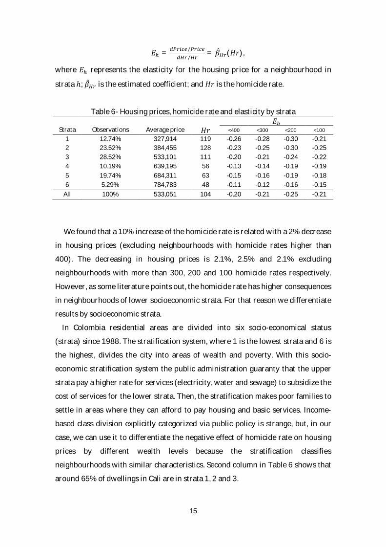
퐸 = ⁄⁄
= 훽 (퐻푟),
where 퐸 represents the elasticity for the housing price for a neighbourhood in
strata ℎ; 훽 is the estimated coefficient; and 퐻푟 is the homicide rate.
Table 6- Housing prices, homicide rate and elasticity by strata 퐸
Strata Observations Average price 퐻푟 <400 <300 <200 <100
1 12.74% 327,914 119 -0.26 -0.28 -0.30 -0.21 2 23.52% 384,455 128 -0.23 -0.25 -0.30 -0.25 3 28.52% 533,101 111 -0.20 -0.21 -0.24 -0.22 4 10.19% 639,195 56 -0.13 -0.14 -0.19 -0.19 5 19.74% 684,311 63 -0.15 -0.16 -0.19 -0.18 6 5.29% 784,783 48 -0.11 -0.12 -0.16 -0.15
All 100% 533,051 104 -0.20 -0.21 -0.25 -0.21
We found that a 10% increase of the homicide rate is related with a 2% decrease
in housing prices (excluding neighbourhoods with homicide rates higher than
400). The decreasing in housing prices is 2.1%, 2.5% and 2.1% excluding
neighbourhoods with more than 300, 200 and 100 homicide rates respectively.
However, as some literature points out, the homicide rate has higher consequences
in neighbourhoods of lower socioeconomic strata. For that reason we differentiate
results by socioeconomic strata.
In Colombia residential areas are divided into six socio-economical status
(strata) since 1988. The stratification system, where 1 is the lowest strata and 6 is
the highest, divides the city into areas of wealth and poverty. With this socio-
economic stratification system the public administration guaranty that the upper
strata pay a higher rate for services (electricity, water and sewage) to subsidize the
cost of services for the lower strata. Then, the stratification makes poor families to
settle in areas where they can afford to pay housing and basic services. Income-
based class division explicitly categorized via public policy is strange, but, in our
case, we can use it to differentiate the negative effect of homicide rate on housing
prices by different wealth levels because the stratification classifies
neighbourhoods with similar characteristics. Second column in Table 6 shows that
around 65% of dwellings in Cali are in strata 1, 2 and 3.

16
Third column in Table 6 shows the average prices of the square meter by strata;
column 4 shows the homicide rate per 100,000 people (it is clear that the rate is
higher in lower strata); and last four columns shows that price-homicide rate
elasticity is more negative in lower strata. In any case, the fact that the elasticity
decreases with strata may result from the definition of elasticity: (Percentage
change price) / (Percentage change homicide rate). This means that if a wealthy
neighbourhood in the homicide rate goes from 1 to 2, the percentage change is
100%. If a very poor neighbourhood in the homicide rate from 100 to 150, the
percentage of variation is 50%. In the end, if in a very wealthy neighbourhood
homicide rate goes from 0 to 1, the percentage of variation is infinite, so that
elasticity must be zero.
In Colombia crime is constant across the income distribution, nevertheless the
rich are most often victims of kidnappings and the poor are most often victims of
homicides. For that reason, rich are more likely to adopt costly protective
behaviour, neighbourhood watch programs, installing anti-theft devices at home,
hiring private security personnel or migrating (Gaviria and Vélez, 2002). In Brazil
homicide victimization is also more common in lower socioeconomic strata
(Soares, 2006). And in Argentina most of the increase in burglary rates was
shouldered by the poor, since the rich were able to adopt effective protective
strategies (Di Tella et al., 2010).
A comment note about endogeneity
The problem of endogeneity arises through the correlation between the regressors
and the random disturbances. Consequently, treating crime rate as exogenous
determinant may have biased the elasticity estimates because crime occurs
disproportionately in poorer neighbourhoods with low housing prices or,
conversely, if criminals target areas where housing prices are higher. In both cases
the behaviour of neighbours will depend on their individual characteristics and
these may well be systematically related to unobserved determinants of housing
prices (Gibbons, 2004; Buonanno, et al., 2013). We may infer a causal relationship
between local characteristics and housing prices, when in fact it is the unobserved
component that drives a neighbourhood composition.

17
Estimate the impact of crime on housing prices is empirically challenging
because of omitted variables, furthermore it is difficult to find valid instruments.
Gibbons (2004) use instruments like: crimes on non-residential properties, spatial
lags of crime, or the distance to nearest public house or wine bar. Buonnano et al.
(2012) uses the victimization rate 20 years ago and the share of youth aged
between 15 and 24 as instruments of crime rates.
In the present paper the explanatory variable refers to homicides, but not theft
or crime in general. Homicide and theft could be correlated, but motives of
homicide may differ from the motivations of theft. Indeed, the propensity to report
a theft varies with the severity of the incidence. Facing the difficulty to find valid
instruments, we have tried to cope with the endogeneity problem by including in
the right hand side of the equation all the variables than may provoke the
correlation between regressors and random disturbances.
4. Conclusions
High homicide rates discourage new residents in a neighbourhood and encourage
those people who can move out to neighbourhoods with lower homicide rate. And
this phenomenon has consequences in the housing market. The objective of the
paper is evaluating the relationship between homicide rates and housing prices in
Cali, Colombia. We use cadastral information of housing prices of 2012 and the
average homicide rates of the period 2000-2010 at neighbourhood level.
The analysis was performed using two estimation strategies. In the first we
estimate a model where the dependent variable is housing prices and one of the
explanation variables is the homicide rate: we found that a 10% increase of the
homicide rate is related with a 2.4% decrease in housing prices. In the second
strategy we estimate a two stage model: in one stage we estimate the hedonic price
at neighbourhood level and next we estimate a regression to test if the homicide
rate has a negative relationship with the estimated hedonic price. We found that, in
average, a 10% increase of the homicide rate is related with a decreasing between
2% and 2.5% in housing prices.
Future work in order to improve estimations will be to include house
characteristics and evaluate strategies to deal with endogeneity problems.

18
References
Atkinson; Healey and Mourato (2005). “Valuing the Cost of Violent Crime: A
Stated Preference Approach”. Oxford Economic Papers, 57, Pp. 559-585.
Besley, Timothy and Mueller, Hannes (2012). “Estimating the Peace Dividend:
The Impact of Violence on Housing Prices in Northern Ireland”. American Economic
Review, 102 (2), Pp. 810-813.
Bowes, Davis and Ihlanfeldt, Keith (2001). “Identifying the Impacts of Rail
Transit Stations on Residential property Values”. Journal of Urban Economics, 50,
Pp. 1-25.
Buonanno; Montolio and Raya-Vílchez (2013). “Housing Prices and Crime
Perception”. Empirical Economics, Vol. 45, Pp. 305-321.
Cameron, Colin and Miller, Douglas (2015). “A Practitioner’s Guide to Cluster-
Robust Inference”. The Journal of Human Resources, 50, Pp. 317-372.
Carson; Flores and Meade (2001). “Contingent Valuation: Controversies and
Evidence”. Environmental and Resource Economics, 19(2), Pp. 173-210.
Ceccato, Vania and Wilhelmsson, Mats (2011). “The Impact of Crime on
Apartment Prices: Evidence from Stockholm, Sweden”. Geografiska Annaler: Series
B, Swedish Society for Antropology and Geography, Pp. 81-103.
CCSP-JP (2015). “Caracas, Venezuela, the Most Violent City in the World”.
Cohen; Rust; Steen and Tidd (2004). “Willingness to Pay for Crime Control
Programs”. Criminology, 42(1), Pp. 89-109.
DAHM (2012). “El Catastro en Cali: Evolución y Recomendaciones de Política”.
Departamento Administrativo de Hacienda Municipal, Alcaldía de Santiago de Cali.
Di Tella, Edwards and Schargrodsky (2010). “”. In The Economics of Crime:
Lessons for and from Latin America, National Bureau of Economic Research.
University of Chicago Press.
Frischtak, Claudio and Mandel, Benjamin (2012). “Crime, House Price, and
Inequality: The Effect of UPPs in Rio”. Federal Reserve Bank of New York Staff
Reports, No. 542.

19
Gaviria, Alejandro and Vélez, Carlos (2002). “Who Bears the Burden of Crime
and Violence in Colombia?”. In Colombia Poverty Report, Vol. 2, 146-161.
Washington, D.C. World Bank.
Gibbons, Steve (2004). “The Cost of Urban Property Crime”. The Economic
Journal, Vol.114, No. 499, Pp. 441-463.
Glaeser, Edward and Sacerdote, Bruce (1999). “Why is there more Crime in
Cities”. Journal of Political Economy, Vol. 107, No. S6, Pp. S225-S258.
Hellman, Daryl and Naroff, Joel (1979). “The Impact of Crime on Urban
Residential Property Values”. Urban Studies, 16, Pp. 105-112.
Levitt, Steven and List, John (2007). “What do Laboratory Experiments
Measuring Social Preferences Reveal about the Real World?”. The Journal of
Economic Perspectives, Vol. 21, No. 2, Pp. 153-174.
Rizzo, Mario (1979). “The Effect of Crime on Residential Rents and Property
Values”. The American Economist, Vol. 23, No. 1, Pp. 16-21.
Rosen, Sherwin (1974). “Hedonic Prices and Implicit Markets: Product
Differentiation in Pure Competition”. Journal of Political Economy, 82(1), Pp. 34-55.
Soares, Rodrigo (2006). “The Welfare Cost of Violence across Countries”.
Journal of Health Economics, Vol. 25 (5), Pp. 821-846.
Soares, Rodrigo (2010). “Welfare Costs of Crime and Common Violence: A
Critical Review”. Pontifical Catholic University of Rio de Janeiro and IZA.
Thaler, Richard (1976). “A Note on the Value of Crime Control: Evidence from
the Property Market”. Journal of Urban Economics, 5, Pp. 137-145.
The Economist (2016). “The World’s most Violent Cities”. February 3rd 2016,
http://www.economist.com/blogs/graphicdetail/2016/02/daily-chart-3
White, Halbert (1980). “A Heteroskedasticity-Consistent Covariance Matrix
Estimator and a Direct Test for Heteroskedasticity”. Econometrica, 48, Pp. 817-838.

20
Annex: Potential consequences on the estimated standard errors derived from forming false clusters
When the statistical information is clustered (e.g. classrooms, neighbourhoods,
economic sectors) the specialized literature recommends to estimate models using
cluster standard errors. In this section we have carried out a simulation exercise to
show potential consequences on the estimated standard errors derived from
forming false clusters. The starting point is the OLS estimation of the regression
model in Table 3:
푦 = 푋훽 + 푢,
where 푦 represents the log of housing price and the explanatory variables are the
area, the squared of the area, and the fixed effects of neighbourhoods. Using the
OLS estimation of 훽 = 훽 and the standard error of disturbances 휎 = 0.39, we
generate a new dependent variable 푦 as follows:
푦 = 푋훽 + 푢 ,
where 푢 is a normal independent random number distribution with a zero mean
and a standard deviation of 휎 = 0.39. These random disturbances verify the
standard hypothesis of the regression model, then, the population matrix of
variances and covariances of the estimated coefficients is obtained as follows:
푐표푣 훽 = (0.39) (푋′푋)
Once the simulated dependent variable, 푦 , has been generated, we estimate
the equation with errors clustered at neighbourhood level, which means that we
are dealing with false clusters. The new estimated covariance matrix is 푐표푣 훽 .
This strategy enables the comparison between the population covariance matrix
푐표푣 훽 and the estimated covariance matrix 푐표푣 훽 . We estimate the equation
with clustered errors 1,000 times. For each standard error of the coefficient, we
calculate the percentage of error, 푝푒 , as follows:
푝푒 =
⎣⎢⎢⎡ 푣푎푟 훽 − 푣푎푟 훽
푣푎푟 훽 ⎦⎥⎥⎤
. 100
Figure 4 presents the percentage of error. The area error seems to be free from
bias, however, the absolute value of the error is 6.3%. The worrying results for the
cluster option are those related to neighbourhood fixed effects, which implies an

21
important negative bias. Figure 1A shows the distributions of the percentage of
error, 푝푒 , for two groups of variables: area of the house and neighbourhood fixed
effects. The average of the distribution of errors for neighbourhood fixed effects is
-96%. The main conclusion is that false cluster can have an important cost,
Nevertheless, in this paper the statistical significance of the coefficients is invariant
to the option selected as is shown in Table 3 of the main text.
Figure 1A-Consequences from forming false clusters
Figure 2A shows results from a similar simulation process using the
heteroskedasticity correction suggested by White (1980). The estimations of the
covariance matrix are denominated robust. As in the previous exercise, the robust
correction is unnecessary but enables to analyze potential effects of making such
corrections.
Figure 2A-Consequences from unnecessary robust correction