3. fundamentals of face recognition...
TRANSCRIPT
71
3. Fundamentals of Face Recognition Techniques
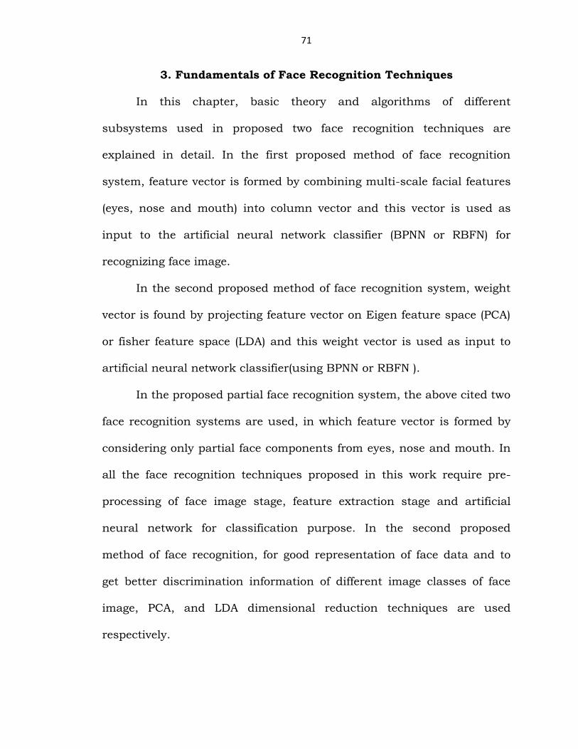
In this chapter, basic theory and algorithms of different
subsystems used in proposed two face recognition techniques are
explained in detail. In the first proposed method of face recognition
system, feature vector is formed by combining multi-scale facial features
(eyes, nose and mouth) into column vector and this vector is used as
input to the artificial neural network classifier (BPNN or RBFN) for
recognizing face image.
In the second proposed method of face recognition system, weight
vector is found by projecting feature vector on Eigen feature space (PCA)
or fisher feature space (LDA) and this weight vector is used as input to
artificial neural network classifier(using BPNN or RBFN ).
In the proposed partial face recognition system, the above cited two
face recognition systems are used, in which feature vector is formed by
considering only partial face components from eyes, nose and mouth. In
all the face recognition techniques proposed in this work require pre-
processing of face image stage, feature extraction stage and artificial
neural network for classification purpose. In the second proposed
method of face recognition, for good representation of face data and to
get better discrimination information of different image classes of face
image, PCA, and LDA dimensional reduction techniques are used
respectively.

72
First part of this chapter describes about different steps involved in
face image pre-processing and feature extraction stages, with the help of
flow charts. Second part of this chapter explains about PCA, LDA and
PCA+ANN, LDA+ANN along with the basics and training algorithms of
Artificial Neural Networks (BPNN and RBFN).
3.1) Pre-Processing of Face Image
In this module, by means of early vision techniques, face images
are pre-processed and enhanced to improve the recognition performance
of the system. Based on requirement some of the following pre-
processing techniques are used in the proposed face recognition
system. Different types of pre-processing/enhancement techniques
related to the face recognition process are explained as fallows with the
help of flow chart and corresponding face images.
73
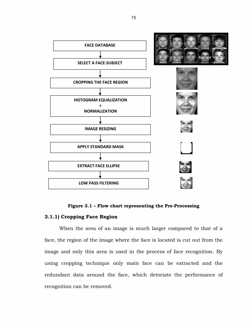
Figure 3.1 – Flow chart representing the Pre-Processing
3.1.1) Cropping Face Region
When the area of an image is much larger compared to that of a
face, the region of the image where the face is located is cut out from the
image and only this area is used in the process of face recognition. By
using cropping technique only main face can be extracted and the
redundant data around the face, which detoriate the performance of
recognition can be removed.
FACE DATABASE
SELECT A FACE-SUBJECT
CROPPING THE FACE REGION
HISTOGRAM EQUALIZATION +
NORMALIZATION
IMAGE RESIZING
APPLY STANDARD MASK
EXTRACT FACE ELLIPSE
LOW PASS FILTERING

74
In this study, the face area is determined manually based on
observation of different face images in the given database and
rectangular or square window corner points are selected in such a way
that it includes main features of face such as eyes, nose, and mouth. All
face images to be trained or tested in recognition process are cropped by
using same corner points („imcrop‟ function in MATLAB is being used for
cropping required part from each face image).
3.1.2) Histogram Equalization
It is usually done on low contrast images in order to enhance
image quality and to improve face recognition performance. It changes
the dynamic range (contrast range) of the image and as a result, some
important facial features become more visible.
Mathematically histogram equalization can be expressed as:
Sk = T rk = n j
n
kj=0 (3.1)
Whereas k=0,1,2,…., L-1
Here in equation (3.1) 'n' is the total number of pixels in an image,
'nj' is the number of pixels with gray level 'rk' ,and 'L' is the total number
of gray levels exist in the face image.
The result after applying histogram equalization to a sample face image is
shown in Figure. 3.2.
75
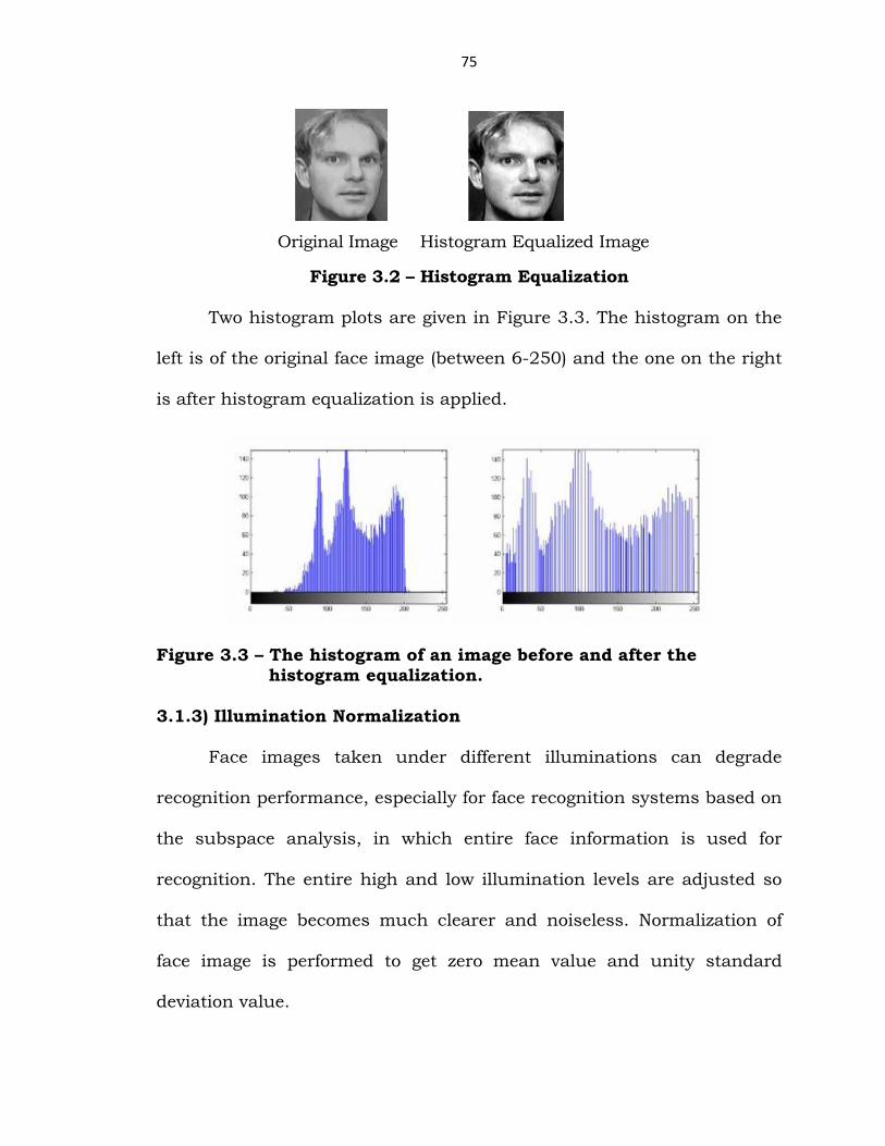
Original Image Histogram Equalized Image
Figure 3.2 – Histogram Equalization
Two histogram plots are given in Figure 3.3. The histogram on the
left is of the original face image (between 6-250) and the one on the right
is after histogram equalization is applied.
Figure 3.3 – The histogram of an image before and after the histogram equalization.
3.1.3) Illumination Normalization
Face images taken under different illuminations can degrade
recognition performance, especially for face recognition systems based on
the subspace analysis, in which entire face information is used for
recognition. The entire high and low illumination levels are adjusted so
that the image becomes much clearer and noiseless. Normalization of
face image is performed to get zero mean value and unity standard
deviation value.

76
3.1.4) Image re-sizing using Bi-Cubic Interpolation method
The process of image resizing changes the size of the image, in this
work, the size of the image is scaled down to reduce the resolution of face
image. This reduction in size is done to reduce mathematical complexity
in PCA/LDA process and neural network training process .For resizing
face image, different interpolation techniques exist in literature ,among
them Bi-cubic interpolation method is being used in the proposed work,
the advantage of resizing through Bi-cubic interpolation is that, it
produces more smoother surfaces than any other interpolation
technique[58] (image is being resized to desired dimension by using
„imresize‟ function in MATLAB) . In Bi-cubic Interpolation technique, it
considers 16 neighboring pixels in the rectangular grid and calculates
weighted average of these pixels to replace them with a single pixel, it is
that pixel, which has got the flavor of all the 16 replaced pixels.
3.1.5) Masking
By using a mask, which simply has a face shaped region, the effect
of background change is minimized. The shape of the mask used in this
study is shown in Figure 3.4.
Figure 3.4 – The shape of the face mask used in the pre-processing

77
3.1.6) Low Pass Filtering
The mean/averaging filter is applied in order to produce the blurry
effect, because in the later stages face recognition algorithm include
step of face image re-sizing ( by using down sampling method) while
maintaining the quality of face image. The 5*5 filter is used for this
process.
R=1
25 25
i=1 𝑍𝑖 (3.2)
Equation (3.2) calculates the average value of the pixels, whereas
'z' is the mask, 'i' are mask elements. The mask is then convolved with
image to produce filtering effect, for a 5*5 mask used in the
implementation, it calculate the average of 25 pixels in that filter mask.
3.2) Feature Extraction using Multi-scaling concept
Figure 3.5 – Flowchart for Multi-scale Feature Extraction
Given face normalized and preprocessed
Perform Feature Extraction
Multi-scaling Different Features
Eyes 1:1
Nose 1:2
Mouth 1:4
Remaining portion 1:8
Converting to Single Image Vector

78
3.2.1) Proposed Method for Feature Extraction
It is generally believed that we human beings put different
emphasis on different parts of face e.g. eyes, nose, cheeks, forehead and
other remaining parts. The existing approaches feature extraction
techniques put same emphasize on all parts of a face and results in
redundancy of image data from discrimination point of view .This method
suffers from unwanted equal weightage on whole face portion of the
image effects recognition rate.
In the proposed approach of feature extraction, four different
facial components - two eyes, nose and mouth of the face are extracted
manually from pre-processed face image (all face images to be trained or
tested in recognition process are cropped by using same corner points,
„imcrop‟ function in MATLAB is being used for cropping required part
from each face image). Dimensionality of these face components are then
reduced by down sampling different face components with different
resolution ratios based on significant of the component in recognition
process. Then feature vector is obtained by scanning two dimensional
image patches of different face components in lexicographical order and
combining them into a column vector. The size of the final image column
vector is N x 1, where N is the total number of pixels obtained from all
the four image patches, N depends on the size of face image, resolution
and down sampling ratios and which is very much less than the original
full image data size. In the proposed work, this feature vector is directly
79
applied to the artificial neural network for classification purpose or after
undergoing through dimensional reduction techniques (PCA or LDA) the
resultant weight vector is given as input to artificial neural network.
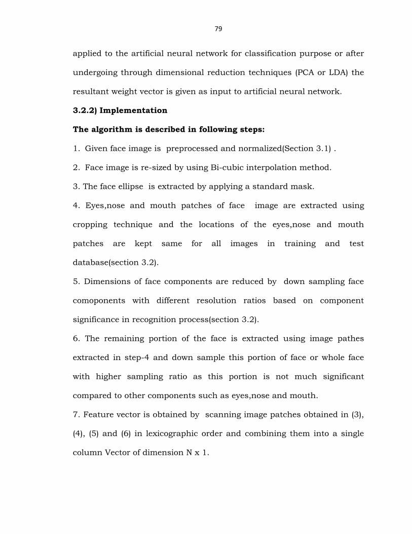
3.2.2) Implementation
The algorithm is described in following steps:
1. Given face image is preprocessed and normalized(Section 3.1) .
2. Face image is re-sized by using Bi-cubic interpolation method.
3. The face ellipse is extracted by applying a standard mask.
4. Eyes,nose and mouth patches of face image are extracted using
cropping technique and the locations of the eyes,nose and mouth
patches are kept same for all images in training and test
database(section 3.2).
5. Dimensions of face components are reduced by down sampling face
comoponents with different resolution ratios based on component
significance in recognition process(section 3.2).
6. The remaining portion of the face is extracted using image pathes
extracted in step-4 and down sample this portion of face or whole face
with higher sampling ratio as this portion is not much significant
compared to other components such as eyes,nose and mouth.
7. Feature vector is obtained by scanning image patches obtained in (3),
(4), (5) and (6) in lexicographic order and combining them into a single
column Vector of dimension N x 1.
80
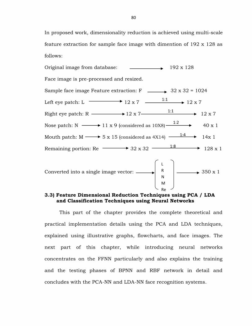
In proposed work, dimensionality reduction is achieved using multi-scale
feature extraction for sample face image with dimention of 192 x 128 as
follows:
Original image from database: 192 x 128
Face image is pre-processed and resized.
Sample face image Feature extraction: F 32 x 32 = 1024
Left eye patch: L 12 x 7 12 x 7
Right eye patch: R 12 x 7 12 x 7
Nose patch: N 11 x 9 (considered as 10X8) 40 x 1
Mouth patch: M 5 x 15 (considered as 4X14) 14x 1
Remaining portion: Re 32 x 32 128 x 1
Converted into a single image vector: 350 x 1
3.3) Feature Dimensional Reduction Techniques using PCA / LDA and Classification Techniques using Neural Networks
This part of the chapter provides the complete theoretical and
practical implementation details using the PCA and LDA techniques,
explained using illustrative graphs, flowcharts, and face images. The
next part of this chapter, while introducing neural networks
concentrates on the FFNN particularly and also explains the training
and the testing phases of BPNN and RBF network in detail and
concludes with the PCA-NN and LDA-NN face recognition systems.
L
R
N
M
Re
1:1
1:1
1:2
1:4
1:8

81
3.3.1) Feature Dimensional Reduction Techniques
Feature selection in pattern recognition technique depends on the
input data feature extraction process and the discrimination power of
features in classification. The number of features required for recognition
process is kept as small as possible due to the measurement cost and
classification accuracy, which also useful to make the system work faster
with minimal memory usage. Continuously, using a wide feature set
causes “curse of dimensionality” being the need for growing number of
samples exponentially [95].
Feature extraction methods use the PCA and LDA methods in
order to reduce the feature dimensions which are mainly used in
classification step [95].
According to the PCA or LDA, the relative places between the data
with respect to feature dimension reduction techniques never changes
and only the axes are being changed which handles the data from a
“better” point of view i.e., the generalization for PCA and discrimination
for LDA.
3.3.1.1) Principal Component Analysis
Under the holistic face recognition method, the principal component
analysis also called karhunen-loeve transformation [96] is used as the
standard technique for statistical pattern recognition process for
dimensional reduction and feature extraction [97], it helps in reducing

82
redundancy while preserving the most intrinsic information content of
the pattern.
A face image which appears in 2-dimension of size N x N can also
be considered as N2 one dimensional vector. Example: face image with
size 112 x 92 under ORL (Olivetti Research Labs) is considered as a
vector having dimensions 10,304, in 10,304 dimensional space. As
image data is not being distributed randomly and exist similarity in the
images of faces, it is possible to describe face image with the low
dimensional subspace techniques like PCA, LDA, and ICA etc.
The main idea of principle component being the vector recognition
is a linear combination of original face images which best accounts for
face image distribution involving the entire image space length N2,
describes an N x N image while defining subspace face image called "face
space.”
Therefore, as these vectors being the eigenvectors of the covariance
matrix corresponding to the original face images and face like in
appearance are referred to as "eigenfaces.”
Considering the training set of face images to be Γ1, Γ2,.., ΓM , the average
of the set can be defined by
Ψ = 1
𝑀 Γ𝑛
𝑀𝑛=1 ----- (3.3)
The vector differentiate each face based on average by
Φi = Γi – Ψ ----- (3.4)

83
This set of large vector, seeks a set of M orthogonal vectors, Um
when subjected to the principal component analysis describing the
distribution of the data. The kth vector, Uk, is chosen such that
𝜆𝑘 = 1
𝑀 𝑈𝑘
𝑇Φn 2𝑀𝑛=1 ------- (3.5)
is a maximum, subjected to
𝑈𝐼𝑇𝑈𝑘 = 𝛿lk =
1, 0,
𝑖𝑓 l = 𝑘𝑜𝑡𝑒𝑟𝑤𝑖𝑠𝑒
------- (3.6)
The vectors Uk and scalars λk can be considered as eigenvectors
and eigenvalues of the covariance matrix respectively
𝐶 = 1
𝑀 ΦnΦ𝑛
𝑇𝑀𝑛=1 = 𝐴𝐴𝑇 ------- (3.7)
Where the matrix A =[Φ1 Φ2....ΦM] however, the covariance matrix
C is N2 x N2 real symmetric matrix, and calculating the N2 eigenvectors
and eigenvalues for such dimension matrix is a difficult task . To reduce
computational complexity in calculating eigenvectors a feasible method
was investigated.
Let v be eigenvectors of ATA such that
𝐴𝑇𝐴𝑣𝑖 = 𝜇𝑖𝑣𝑖 ------- (3.8)
Multiplying both sides by A, we have
𝐴𝐴𝑇𝐴𝑣𝑖 = 𝜇𝑖𝐴𝑣𝑖 ------- (3.9)
Where, it can be found that Avi are the eigenvectors and 𝜇𝑖 are the
eigenvalues of C= A AT.
Following the above analysis, an M X M matrix L= ATA is
constructed ,where Lmn=ΦmTΦn and the M eigenvectors, vi of L are found

84
which determine the linear combinations of the M training set face
images forming the eigenfaces Ui.
𝑈𝑖 = vlk
𝑀
𝑘=l
Φnk , l = 1, … … , M − − − − − − − (3.10)
Using the above analysis, the calculations are reduced drastically
from the order of image dimension (N2) to order of the number of images
in training set (M). Most of the face recognition cases, the training set of
face images are relatively small compared to face image dimension (M
<< N2) and calculations also get reduced to manageable level. In order to
distinguish the variation among the images, the eigenvalues are useful to
rank the eigenvectors. Sirovich & Kirby [24] evaluated a limited version of
the above mentioned framework on 115 image database (M = 115), which
are digitized in a controlled manner and found that the 40 eigenfaces (M'
= 40) are sufficient for describing the face image. In practice, as accurate
reconstruction of the face image is not a required, a smaller M' is found
to be sufficient for recognition. As the eigenfaces span an M' dimensional
subspace of the original N2 image space, the M' significant eigenvectors
of the L matrix having the largest eigenvalues are sufficient for
representation of the reliable faces in face space, which are
characterized by eigenfaces. Examples of ORL face database and
eigenfaces after the application of eigenface algorithms are shown in
Figure 3.6 and Figure 3.7, respectively.

85
Figure 3.6 – Samples face images from the ORL database
By applying a simple operation, a new face image (Γ) can be
transformed into its eigenface components (projected onto "face space"),
𝑤𝑘 = 𝑈𝑘𝑇(Γ − Ψ) ------- (3.11)
for k = 1,...,M'. The weights form a projection vector,
ΩT = [w1, w2, … , wM] ------- (3.12)
Treating the eigenfaces as a basis set of face image, the
description of contribution of each eigenface in the input face
image becomes easy. The projection vector is later used for
standard pattern recognition algorithm as input to the classifier.
The face class Ωk is an average of the eigenface representation
over the small number of sample face images in each class.
Performance of classification measured based on the comparison
between the projection vectors of the training face images with

86
respect to the projection vectors of the input face image by
finding Euclidean Distance between the face classes and the
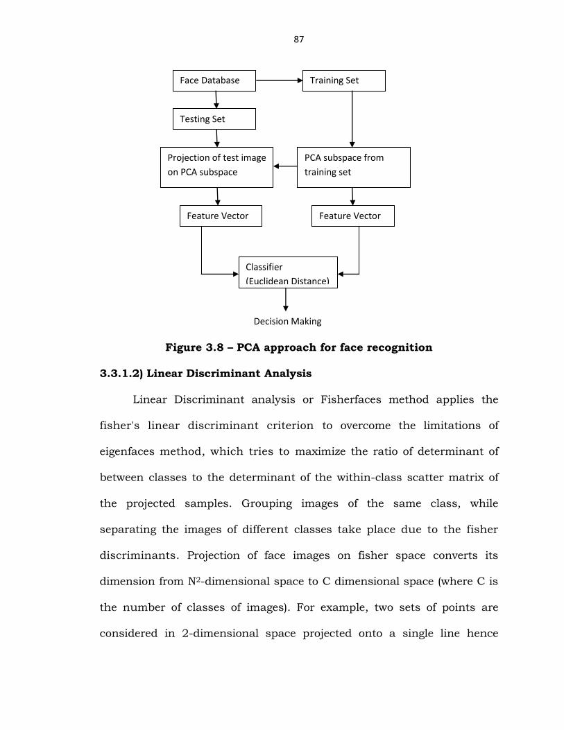
input face image. Henceforth, the major idea is to trace the face
class k which minimizes the Euclidean Distance. Figure 3.8
represents the testing phase of PCA approach.
휀𝑘 = Ω − Ω𝑘 ------- (3.13)
Where Ωk is a vector describing the kth faces class.
Figure 3.7 – First 16 eigenfaces with highest eigenvalues
87
Figure 3.8 – PCA approach for face recognition
3.3.1.2) Linear Discriminant Analysis
Linear Discriminant analysis or Fisherfaces method applies the
fisher's linear discriminant criterion to overcome the limitations of
eigenfaces method, which tries to maximize the ratio of determinant of
between classes to the determinant of the within-class scatter matrix of
the projected samples. Grouping images of the same class, while
separating the images of different classes take place due to the fisher
discriminants. Projection of face images on fisher space converts its
dimension from N2-dimensional space to C dimensional space (where C is
the number of classes of images). For example, two sets of points are
considered in 2-dimensional space projected onto a single line hence
Face Database Training Set
Testing Set
Projection of test image
on PCA subspace
PCA subspace from
training set
Feature Vector Feature Vector
Classifier
(Euclidean Distance)
Decision Making

88
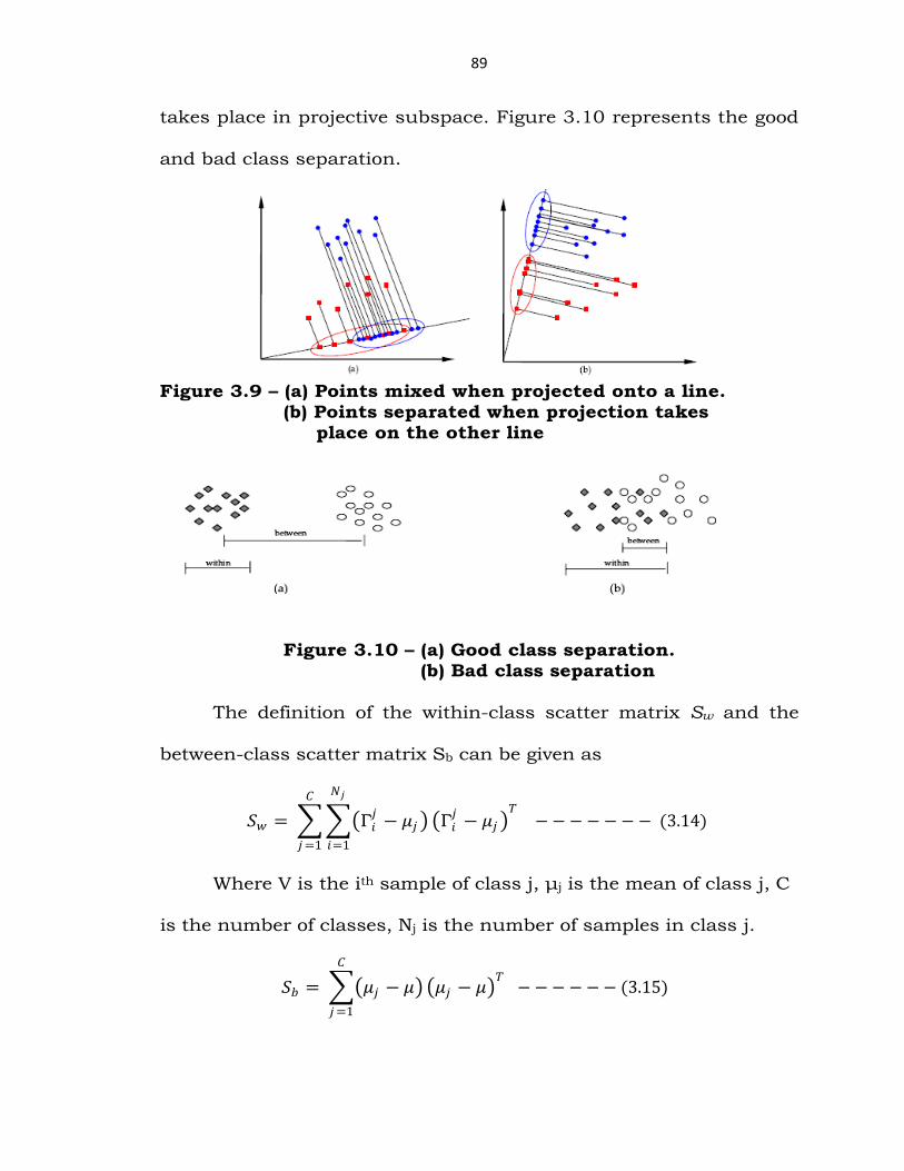
depending on the direction the points are either mixed (Figure 3.9a) or
separated (Figure 3.9b). The fisher discriminate to find the line which
best separates the points i.e., in order to identify the input test image,
the comparison of the projected test image with each training image
takes place after which the test image as the closest training image can
be identified.
Along with eigenspace projection, the training images are also
being projected into a subspace. The test images being projected at the
same subspace can be identified using a similarity measure and the only
difference is the way in the subspace calculations take place.
The PCA method is used to extract features which represents face
image and the LDA method discriminates different face classes in order
to find the subspace as shown in Figure 3.9. The within class scatter
matrix also named as intra-personal shows the variations due to the
different lighting and face expression in the appearance of the same
individual where as the between-class scatter matrix i.e., the extra-
personal represents the variations due to identity differences.
Henceforth, by applying the above mentioned methods, the
projection directions on one hand maximize the distance between
the face images of different classes, while on the other hand it
minimizes the distance between the face images of same class i.e.,
it can also be said that by maximizing the between- class scatter
matrix Sb, while minimizing the within-class scatter matrix Sw
89
takes place in projective subspace. Figure 3.10 represents the good
and bad class separation.
Figure 3.9 – (a) Points mixed when projected onto a line. (b) Points separated when projection takes place on the other line
Figure 3.10 – (a) Good class separation. (b) Bad class separation
The definition of the within-class scatter matrix Sw and the
between-class scatter matrix Sb can be given as
𝑆𝑤 = Γ𝑖𝑗− 𝜇𝑗
𝑁𝑗
𝑖=1
𝐶
𝑗 =1
Γ𝑖𝑗− 𝜇𝑗
𝑇 − − − − − − − (3.14)
Where V is the ith sample of class j, μj is the mean of class j, C
is the number of classes, Nj is the number of samples in class j.
𝑆𝑏 = 𝜇𝑗 − 𝜇
𝐶
𝑗 =1
𝜇𝑗 − 𝜇 𝑇
− − − − − − (3.15)
90
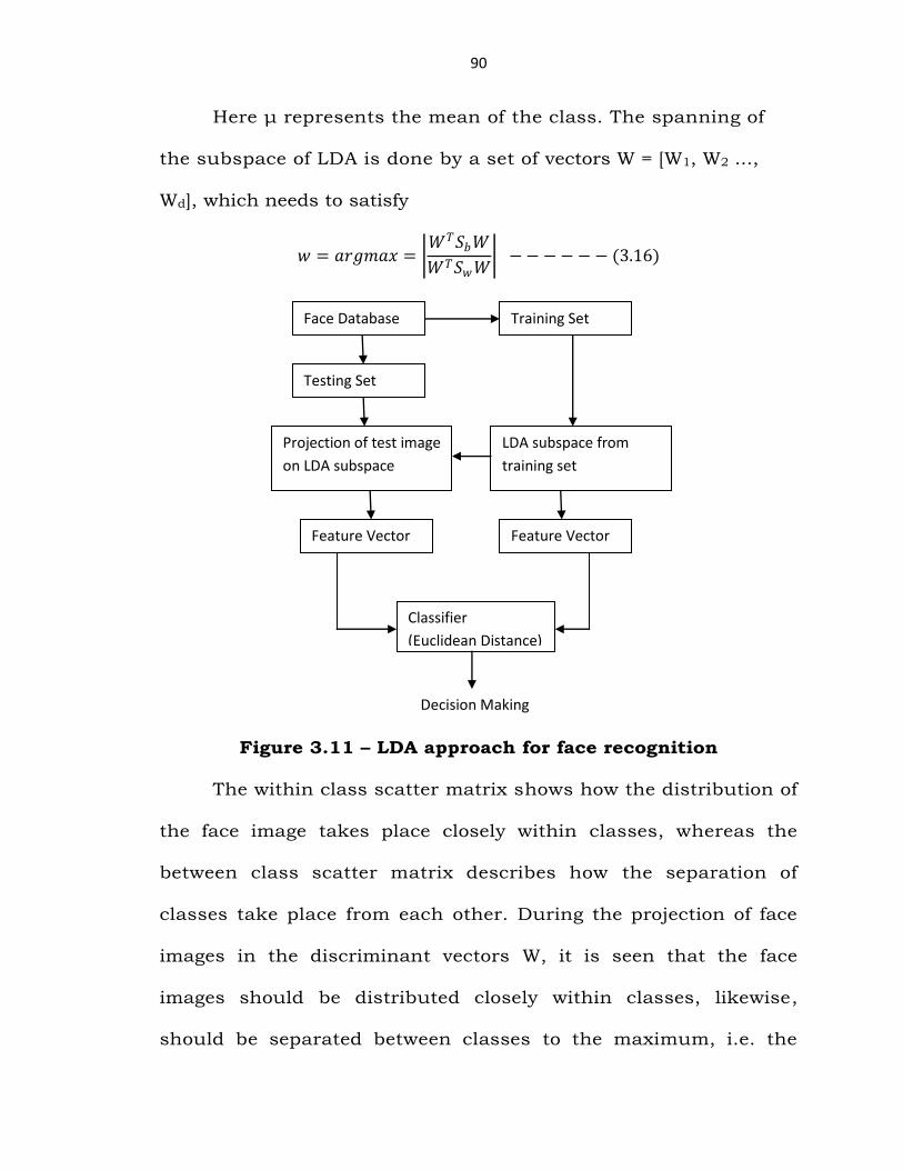
Here μ represents the mean of the class. The spanning of
the subspace of LDA is done by a set of vectors W = [W1, W2 ...,
Wd], which needs to satisfy
𝑤 = 𝑎𝑟𝑔𝑚𝑎𝑥 = 𝑊𝑇𝑆𝑏𝑊
𝑊𝑇𝑆𝑤𝑊 − − − − − − (3.16)
Figure 3.11 – LDA approach for face recognition
The within class scatter matrix shows how the distribution of
the face image takes place closely within classes, whereas the
between class scatter matrix describes how the separation of
classes take place from each other. During the projection of face
images in the discriminant vectors W, it is seen that the face
images should be distributed closely within classes, likewise,
should be separated between classes to the maximum, i.e. the
Face Database Training Set
Testing Set
Projection of test image
on LDA subspace
LDA subspace from
training set
Feature Vector Feature Vector
Classifier
(Euclidean Distance)
Decision Making

91
discriminant vector is responsible for minimizing the
denominator and maximizing the numerator in Equation (3.16).
Therefore, the construction of W takes place with the help of
eigenvectors also called as fisher faces of Sw-1 Sb. There are
various other methods in order to solve the problem of LDA
example: the pseudo inverse method, the subspace method and
the null space method.
The LDA approach being similar to the eigenface method
uses projection of training images into subspace. The test images
are projected into the same subspace and identified using a
similarity measure. The only difference is the method of calculating
the subspace characterizing the face space. The face which has the
minimum distance with the test face image is labeled with the
identity of that image. The minimum distance can be calculated
using the Euclidian distance method as given earlier in Equation (3.13).
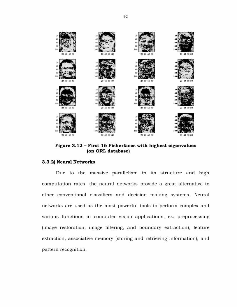
Figure 3.11 shows the testing phase of the LDA approach. Figure 3.12
shows the first 16 Fisherfaces with highest eigenvalues.
92
Figure 3.12 – First 16 Fisherfaces with highest eigenvalues (on ORL database)
3.3.2) Neural Networks
Due to the massive parallelism in its structure and high
computation rates, the neural networks provide a great alternative to
other conventional classifiers and decision making systems. Neural
networks are used as the most powerful tools to perform complex and
various functions in computer vision applications, ex: preprocessing
(image restoration, image filtering, and boundary extraction), feature
extraction, associative memory (storing and retrieving information), and
pattern recognition.

93
3.3.2.1) Significance of Neural Networks in Pattern Recognition
The main characteristics of neural networks are that they have the
ability to learn complex nonlinear input-output relationships, use
sequential training procedures, and adapt themselves to the data. The
most commonly used family of neural networks for pattern classification
tasks is the feed-forward network, which includes multilayer perceptron
and Radial-Basis Function (RBF) networks. Another popular network is
the Self-Organizing Map (SOM), or Kohonen-Network, which is mainly
used for data clustering and feature mapping. The learning process
involves updating network architecture and connection weights so that a
network can efficiently perform a specific classification/clustering task.
The increasing popularity of neural network models to solve pattern
recognition problems has been primarily due to their seemingly low
dependence on domain-specific knowledge and due to the availability of
efficient learning algorithms for practitioners to use. Artificial neural
networks (ANNs) provide a new suite of nonlinear algorithms for feature
extraction (using hidden layers) and classification (e.g., multilayer
perceptrons). In addition, existing feature extraction and classification
algorithms can also be mapped on neural network architectures for
efficient (hardware) implementation. An ANN is an information
processing paradigm that is inspired by the way biological nervous
systems, such as the brain, process information. The key element of this
paradigm is the novel structure of the information processing system. It

94
is composed of a large number of highly interconnected processing
elements (neurons) working in unison to solve specific problems. An ANN
is configured for a specific application, such as pattern recognition or
data classification, through a learning process. Learning in biological
systems involves adjustments to the synaptic connections that exist
between the neurons.
3.3.2.2) Feed Forward Neural Networks (FFNN)
Architecture of Feed forward Neural Networks (FFNN) is more
appropriate configuration for face recognition, where neurons are inter-
connected to form a layer for nonlinear separable input data. Each layer
in network gets input from the previous layer and feed its output to the
next layer but the connections to the neurons in the same or previous
layers are not permitted. Figure 3.13 represents the architecture of the
system for face classification.
Figure 3.13 – Architecture of FFNN for classification

95
In FFNN, the neurons are interconnected in the form of layers and
require a training procedure, in which the weights connected between
consecutive layers are calculated based on both i.e., the training
samples and target classes. The weight vector obtained by projecting
training face image on eigenspace or fisherspace is used as input to
artificial neural network classifier. These methods are called PCA-NN and
LDA-NN for Eigen faces and fisher faces techniques respectively.
3.3.2.3) Learning Algorithm (Backpropagation)
Back propagation learning process requires pairs of input
and target vectors in multi-layer neural network. The difference
between output vector corresponding to each input vector and
the target vector is calculated, and the weights of the network are
adjusted to minimize the difference to the specified threshold
value. Initially, though the random weights and thresholds are
assigned to the network they are updated for every iteration in
order to minimize the function or the mean square error between
the output vector and the target vector. Input for hidden layer is
calculated as
𝑛𝑒𝑡𝑚 = 𝑥2
𝑛
𝑧=1
𝑤𝑚𝑧 − − − − − (3.17)
After passing through the activation function the output
vector of hidden layer is given by
𝑚 =1
1 + exp(−𝑛𝑒𝑡𝑚) − − − −(3.18)

96
Similarly, the input for the output layer is given by
𝑛𝑒𝑡𝑘 = 2
𝑚
𝑧=1
𝑤𝑘𝑧 − − − − − (3.19)
output layer outputs are given by
𝑜𝑘 =1
1 + exp(−𝑛𝑒𝑡𝑘) − − − −(3.20)
for updating the weights, the error is calculated as follows
𝐸 =1
2 (𝑜𝑖 −
𝑘
𝑖=1
𝑡𝑖)2 − − − − − (3.21)
The training process stops if the error is minimum when
compared to the predefined limit else the weights are updated till
error reaches its threshold value. The change in weights between
the input layer and hidden layer is given as follows
Δ𝑤𝑖𝑗 = 𝛼𝛿𝑖𝑗 − − − − − (3.22)
Here, α is a training rate coefficient and is specified to the
range [0.01, 1.0], hj is the output jth neuron in the hidden layer
and δi is given by
𝛿𝑖 = 𝑡𝑖 − 𝑜𝑖 𝑜𝑖 l − 𝑜𝑖 − − − − − (3.23)
oi represents the real output and U is the target output of
ith neuron in the output layer respectively.
Likewise, the change of the weights between hidden layer
and output layer is
Δ𝑤𝑖𝑗 = 𝛽𝛿𝐻𝑖𝑥𝑗 − − − − − (3.24)
97
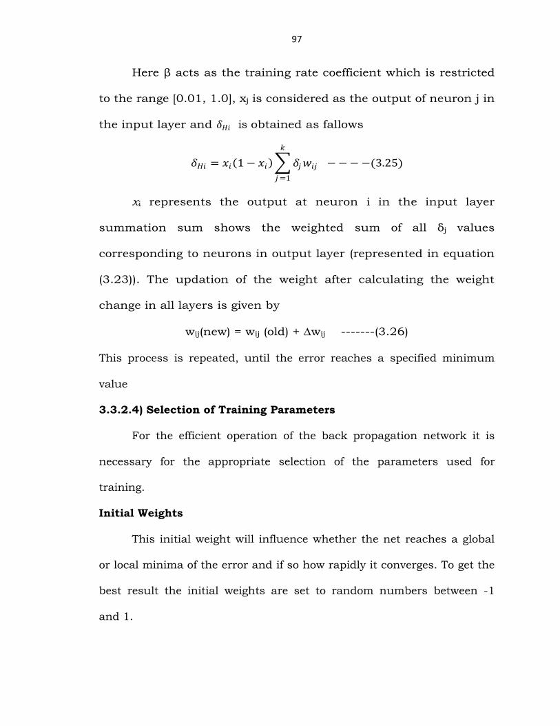
Here β acts as the training rate coefficient which is restricted
to the range [0.01, 1.0], xj is considered as the output of neuron j in
the input layer and 𝛿𝐻𝑖 is obtained as fallows
𝛿𝐻𝑖 = 𝑥𝑖 1 − 𝑥𝑖 𝛿𝑗𝑤𝑖𝑗
𝑘
𝑗 =1
− − − −(3.25)
xi represents the output at neuron i in the input layer
summation sum shows the weighted sum of all δj values
corresponding to neurons in output layer (represented in equation
(3.23)). The updation of the weight after calculating the weight
change in all layers is given by
wij(new) = wij (old) + wij -------(3.26)
This process is repeated, until the error reaches a specified minimum
value
3.3.2.4) Selection of Training Parameters
For the efficient operation of the back propagation network it is
necessary for the appropriate selection of the parameters used for
training.
Initial Weights
This initial weight will influence whether the net reaches a global
or local minima of the error and if so how rapidly it converges. To get the
best result the initial weights are set to random numbers between -1
and 1.

98
Training a Net
The motivation for applying back propagation net is to achieve a
balance between memorization and generalization; it is not necessarily
advantageous to continue training until the error reaches a minimum
value. The weight adjustments are based on the training patterns. As
along as error the for validation decreases training continues. Whenever
the error begins to increase, the net is starting to memorize the training
patterns. At this point training is terminated.
Number of Hidden Units
If the activation function can vary with the function, then it can be
seen that a n-input, m-output function requires at most 2n+1 hidden
units. If more number of hidden layers are present, then the calculation
for the ‟s are repeated for each additional hidden layer present,
summing all the ‟s for units present in the previous layer that is fed into
the current layer for which is being calculated.
Learning rate
In BPN, the weight change is in a direction that is a combination of
current gradient and the previous gradient. A small learning rate is used
to avoid major disruption of the direction of learning when very unusual
pair of training patterns is presented.
Various parameters assumed for different Artificial Neural
Networks are specified in subsequent sections.

99
Main advantage of this back propagation algorithm is that it can
identify the given image as a face image or non face image and then
recognizes the given input image .Thus the back propagation neural
network classifies the input image as recognized image.
3.3.2.5) Radial Basis Function Networks
Though the Radial Basis Function (RBF) network has its own
structure and function, its functionality in mapping is similar to the
multi-layer neural network. RBFN is a local network, while MLNN is a
global network. The global and local networks are differentiated based on
the extension of input surface covered by the function approximation.
RBFN performs a local mapping, in which only nearer inputs to a
respective field produce an activation [98, 99].
The most typical RBF neural network structure can be represented in
Figure 3.14 as
Figure 3.14 – RBF network structure
The input layer of this network consists of n units, and accepts the
elements of an n -dimensional input feature vector. n elements of the
input vector xn goes as input to the l hidden function, i.e., output of the
100
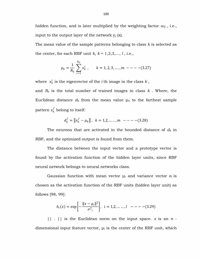
hidden function, and is later multiplied by the weighting factor wij , i.e.,
input to the output layer of the network yj (x).
The mean value of the sample patterns belonging to class k is selected as
the center, for each RBF unit k, k = 1,2,3,..., l , i.e.,
𝜇𝑘 =1
𝑁𝑘 𝑥𝑘
𝑖
𝑁𝑘
𝑖=1
, 𝑘 = 1, 2, 3, … . , 𝑚 − − − −(3.27)
where 𝑥𝑘𝑖 is the eigenvector of the i th image in the class k ,
and Nk is the total number of trained images in class k . Where, the
Euclidean distance dk from the mean value μk to the farthest sample
pattern 𝑥𝑘𝑓 belong to itself:
𝑑𝑘𝑓
= 𝑥𝑘𝑓
− 𝜇𝑘 , 𝑘 = 1,2, … . . , 𝑚 − − − −(3.28)
The neurons that are activated in the bounded distance of dk in
RBF, and the optimized output is found from them.
The distance between the input vector and a prototype vector is
found by the activation function of the hidden layer units, since RBF
neural network belongs to neural networks class.
Gaussian function with mean vector μi and variance vector σi is
chosen as the activation function of the RBF units (hidden layer unit) as
follows [98, 99]:
𝑖 𝑥 = exp − 𝑥 − 𝜇𝑖
2
𝜎2𝑖
, 𝑖 = 1,2, …… , 𝑙 − − − −(3.29)
|| . || is the Euclidean norm on the input space. x is an n -
dimensional input feature vector, μi is the center of the RBF unit, which

101
is an n -dimensional vector, σi is the width of the i th RBF unit and
number of the RBF units is l. For input x, the response of j th output is
given as:
𝑦𝑗 𝑥 = 𝑖 𝑥 𝑤𝑖𝑗
𝑙
𝑖=1
− − − − − (3.30)
where wij is the connection weight of the i -th RBF unit to the j -th output
node.
In order to design a RBF neural network classifier, the number of
the input data elements xi should be equal to the number of the feature
vector elements, likewise the number of the outputs should be equal to
the number of the face classes in the face image database considered for
training.
The implementation of the learning algorithm for radial basis
function network is done in two stages. In the first stage of learning, the
number of radial basis functions and their center values are calculated.
Whereas in the second stage, by using gradient descent or a least-square
algorithm the weights connecting to layers L1 and L2 are calculated.
The learning algorithm using the gradient descent method is as
follows [100,101]:
1. Initial weights wij are assigned with small random values and the
radial basis function hj are defined, using the mean μj, and standard
deviation σj.
2. Output vectors h and y are obtained using (3.29) and (3.30).

102
3. Change in weight is Calculated as Δwij =α (ti – yi )hj .
where α is a constant, ti is the target output, and oi is the actual output.
4. Weights are updated by using wij (k +1) = wij (k) + Δwij.
5. Mean square error is calculated by using 𝐸 =1
2 𝑡𝑖 − 𝑦𝑖
2𝑚𝑖=1
6. Steps 2 to5 are repeated until min E ≤ Emin.
7. Steps 2-6 are repeated for all training samples.
The output layer is a layer of standard linear neurons performs a
linear transformation of the hidden node outputs. It is equivalent to a
linear output layer in a MLNN and a gradient descent algorithm is used
to train the weights. The biases may/may not be present in the output
layer.
Receptive fields concentrates on the areas of the input space where
the input vectors exists and cluster the similar input vector. The hidden
node will be activated when the input vector (x) lies near the center of a
receptive field (μ). No activation of both the hidden nodes takes place in
case the input vector lies between two receptive fields where as the input
vector lie far from all the receptive fields. Hence, here the RBF output is
equal to that of the output layer bias values [102] which is a local
network trained in a supervised manner. The RBF contrasts with the
MLNN network which is itself a global network. Inspite of extent of input
surface which is covered by the function approximation there exists
discrimination between the local and global network. MLNN performs a
global mapping i.e., all inputs cause on output whereas an RBF performs

103
a local mapping which causes the activation of all inputs near the
receptive field take place.
3.4) Face Databases
The experiments are conducted on the FERET & ORL face image
databases in the proposed work, as most of the researchers in literature
used same data base for comparing performance different face
recognition techniques.
3.4.1) FERET database
In FERET database images are acquired under variable pose, facial
expressions, illumination, with and without spectacles during different
photo sessions, and in this study upto 500 frontal face images of 100
subjects are used, each with 5 variations (as shown in figure-3.15).
Figure: 3.15 – Sample face images in FERET database
3.4.2) ORL Database
The ORL database contains 10 different face images of 40 distinct
subjects. The images vary in terms of pose, facial expressions, lighting,
with and without spectacles during different photo sessions. Figure
3.16 shows sample images of a single subject in ORL database.

104
Figure 3.16 – Sample face images in ORL data base
3.5) Conclusions
In this chapter, the introductions of the main subsystems used in
the proposed face recognition systems are explained in detail. In the
proposed face recognition systems mainly consists of fallowing stages:
pre-processing, feature extraction, dimensional reduction and
classification using artificial neural networks. Hence, in this chapter,
different face image pre-processing techniques: average filtering, image
resizing, histogram equalization, intensity normalization, and image
cropping techniques are explained. In dimensional reduction techniques
PCA and LDA algorithms are explained. Under the databases used in
proposed work, ORL and FERET databases have been explained. In the
end, training algorithms for BPNN and RBFN are explained.