3. formal quantum theory

3. Formal Quantum Theory

Background

A modern physics course

Quantum harmonic oscillator and the hydrogen atom

Vector spaces

Eigenvalue problems

Concepts of primary interest:

Sample calculations:

SC1 -

Helpful handouts:

Hermite Polynomials

Vector spaces handout

Matrices and eigenvalue problems handout

Appendices:

Plots for problem GQM3.28

Notation for a matrix representation of the vector space

*** Review of the dagger operation 0

0

ˆ ( )( ) ( )

i H t tt t e

Change of Basis Transformation

Tools of the trade:

Time development of an arbitrary wavefunction

Matrix example of the time development of an arbitrary wavefunction

This handout is keyed to Griffiths Introduction to Quantum Mechanics, 2nd Ed. It is

not designed to be used independently.

for use with Griffiths QM Contact: [email protected]

I think I can safely say that nobody understands Quantum Mechanics.

Richard Feynman

If you thought that science was certain - well, that is just an error on your part.

Richard Feynman

Notation/convention Alert:

This formal quantum theory section is focused on operators and wavefunctions. The

physically admissible wavefunctions are vectors in a linear vector space. As you study

the text, it is important to remember that the handouts have used several terms in

unconventional ways. First, the term linear operator is used to identify a linear

transformation that acts of a vector in the space and returns another vector in that same

space. In this role, a hamiltonian acting on a wavefunction to return an energy-valued

constant times the original wavefunction is acceptable. Our view is that the state is the

normalized wavefunction, and normalization resets the dimensions of the function to

[density]-½. The math aspects of quantum theory have no regard for dimensions in the

sense of mass, length, time, … . In mathspeak, a linear operator is a linear

9/20/2010 SP425 Notes –Formal Quantum Theory Ch3-2

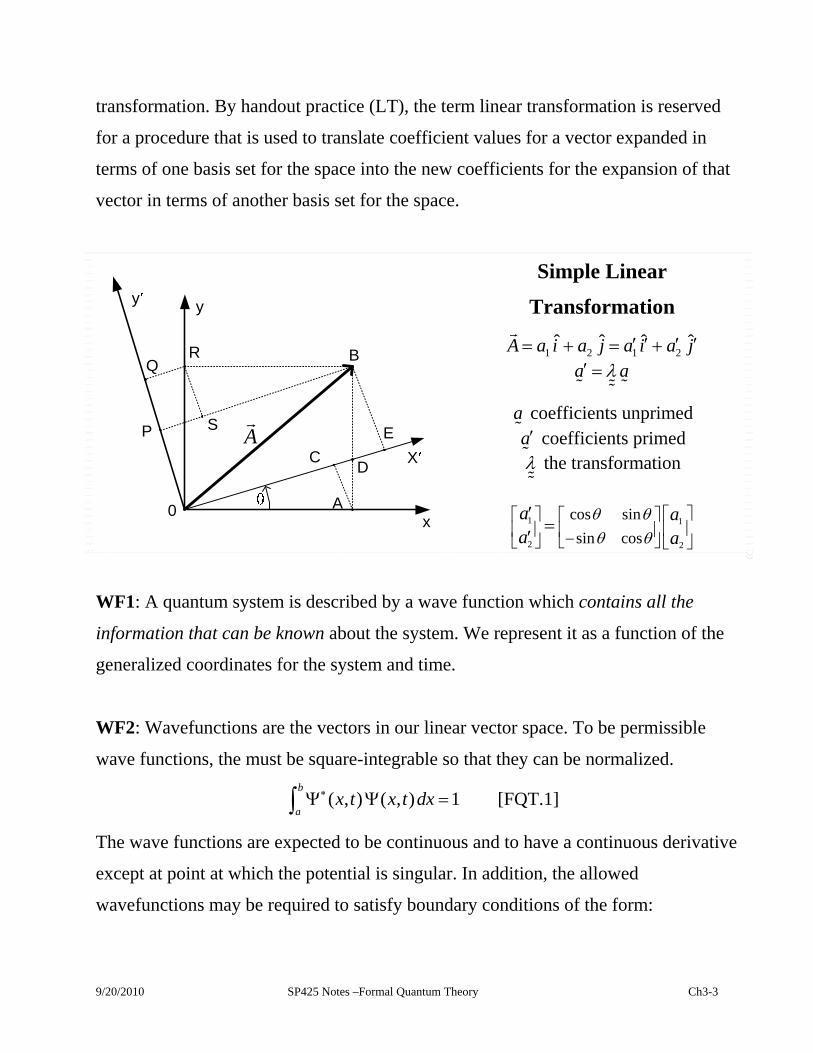
transformation. By handout practice (LT), the term linear transformation is reserved

for a procedure that is used to translate coefficient values for a vector expanded in

terms of one basis set for the space into the new coefficients for the expansion of that

vector in terms of another basis set for the space.

R

SP

QB

E

CD

A

y

x

X

y

0

A

Simple Linear

Transformation

1 2 1 2ˆ ˆ ˆ ˆA a i a j a i a j

a a

aa coefficients unprimed

coefficients primed

the transformation

1 1

2 2

cos sin

sin cos

a aa a

WF1: A quantum system is described by a wave function which contains all the

information that can be known about the system. We represent it as a function of the

generalized coordinates for the system and time.

WF2: Wavefunctions are the vectors in our linear vector space. To be permissible

wave functions, the must be square-integrable so that they can be normalized.

( , ) ( , ) 1b

ax t x t dx [FQT.1]

The wave functions are expected to be continuous and to have a continuous derivative

except at point at which the potential is singular. In addition, the allowed

wavefunctions may be required to satisfy boundary conditions of the form:


( , ) ( , ) 0x b x ax xx t x t

km

. [FQT.2]

While we are to be extremely suspicious of wavefunctions lacking these properties,

they may be useful in special circumstances.

It is assumed that we can find a set of wavefunctions { … , k, … } that are

orthonormal and that serve as a basis for the complete set of permissible solutions.

( , ) ( , )b

k max t x t dx (Kronecker-like)

Exercise: Give two examples with wavefunctions that are not differentiable at a point

and describe the singular behavior of the potential at that point.

As wavefunctions are to be unity normalized, one might just say that the magnitude of

the wavefunction is to be ignored and that the ‘direction’ of the state carries all the

quantum information.

There are cases when generalized wavefunctions prove to be useful. In fact, they arise

whenever the spectrum of eigenvalues is continuous. Confinement (or limited range)

ensures that an eigenvalues are discrete so a continuous spectrum indicates the absence

of confinement. The probability amplitude (wavefunction) spreads out and is un-

confined, and hence it is not normalizable. The eigenstates of linear momentum have a

zero uncertainty in momentum and hence have an infinite spatial spread of the

conjugate coordinate. A precise px is tied to an infinite x. Such states cannot be

normalized.

( )12

ˆ ( , ) i kx tp kxp i x t e

The function is not normalizable, but it does conform to a Dirac normalization.


2 21 1( ,0) ( ,0) ( )ikx ik x

p k p kx x dx e e dx k k

(Dirac)

Orthogonality for a continuous rather than discrete eigenvalue spectrum

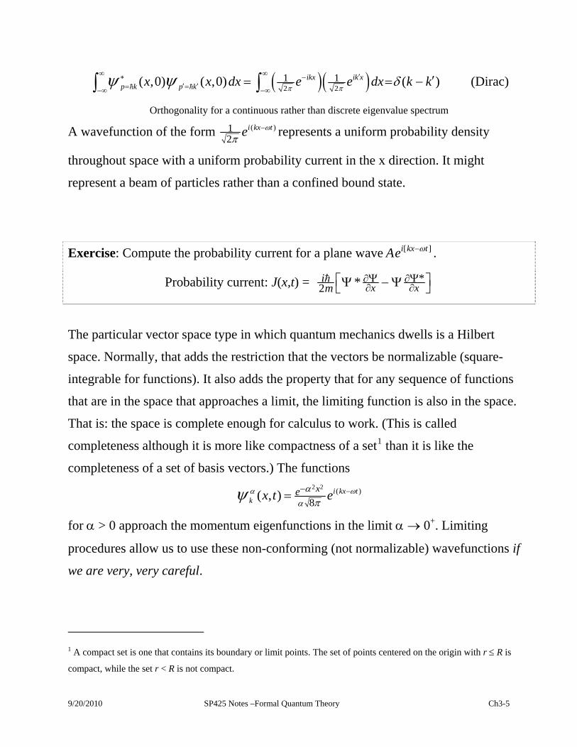
A wavefunction of the form (12

i kx te )

represents a uniform probability density

throughout space with a uniform probability current in the x direction. It might

represent a beam of particles rather than a confined bound state.

Exercise: Compute the probability current for a plane wave [ ]i kx tAe .

Probability current: J(x,t) = *2 * x xim

The particular vector space type in which quantum mechanics dwells is a Hilbert

space. Normally, that adds the restriction that the vectors be normalizable (square-

integrable for functions). It also adds the property that for any sequence of functions

that are in the space that approaches a limit, the limiting function is also in the space.

That is: the space is complete enough for calculus to work. (This is called

completeness although it is more like compactness of a set1 than it is like the

completeness of a set of basis vectors.) The functions 2 2

( )

8( , ) i kx t

k

xex t e

for > 0 approach the momentum eigenfunctions in the limit 0+. Limiting

procedures allow us to use these non-conforming (not normalizable) wavefunctions if

we are very, very careful.

1 A compact set is one that contains its boundary or limit points. The set of points centered on the origin with r R is

compact, while the set r < R is not compact.


As quantum mechanics is probabilistic, and the theory does not provide answers for

every question that you might conceive. Each observable (or question that can be

answered) has an associated Hermitian operator.

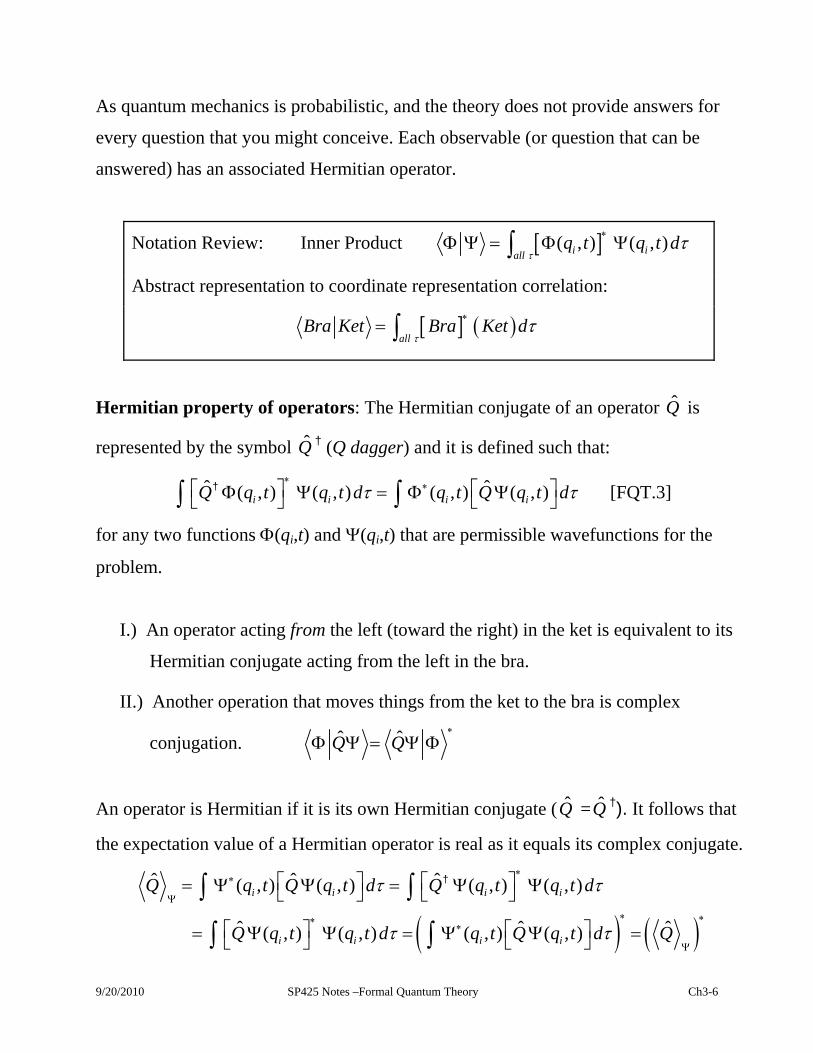
Notation Review: Inner Product ( , ) ( , )i iallq t q t d

Abstract representation to coordinate representation correlation:

all

Bra Ket Bra Ket d

Hermitian property of operators: The Hermitian conjugate of an operator is

represented by the symbol † (Q dagger) and it is defined such that:

Q

Q

ˆ ˆ( , ) ( , ) ( , ) ( , )i i i iQ q t q t d q t Q q t d

† [FQT.3]

for any two functions (qi,t) and (qi,t) that are permissible wavefunctions for the

problem.

I.) An operator acting from the left (toward the right) in the ket is equivalent to its

Hermitian conjugate acting from the left in the bra.

II.) Another operation that moves things from the ket to the bra is complex

conjugation. ˆ ˆQ Q

An operator is Hermitian if it is its own Hermitian conjugate ( = †). It follows that

the expectation value of a Hermitian operator is real as it equals its complex conjugate.

Q Q

ˆ ˆ ˆ( , ) ( , ) ( , ) ( , )

ˆ ˆ( , ) ( , ) ( , ) ( , )

i i i i

i i i i

Q q t Q q t d Q q t q t d

Q q t q t d q t Q q t d Q

ˆ

†


Eigenfunctions of a Hermitian operator that have distinct eigenvalues are orthogonal.

If there is an m-fold degenerate eigenvalue, m mutually orthogonal eigenfunctions can

be constructed as linear combinations of the original m independent solutions.

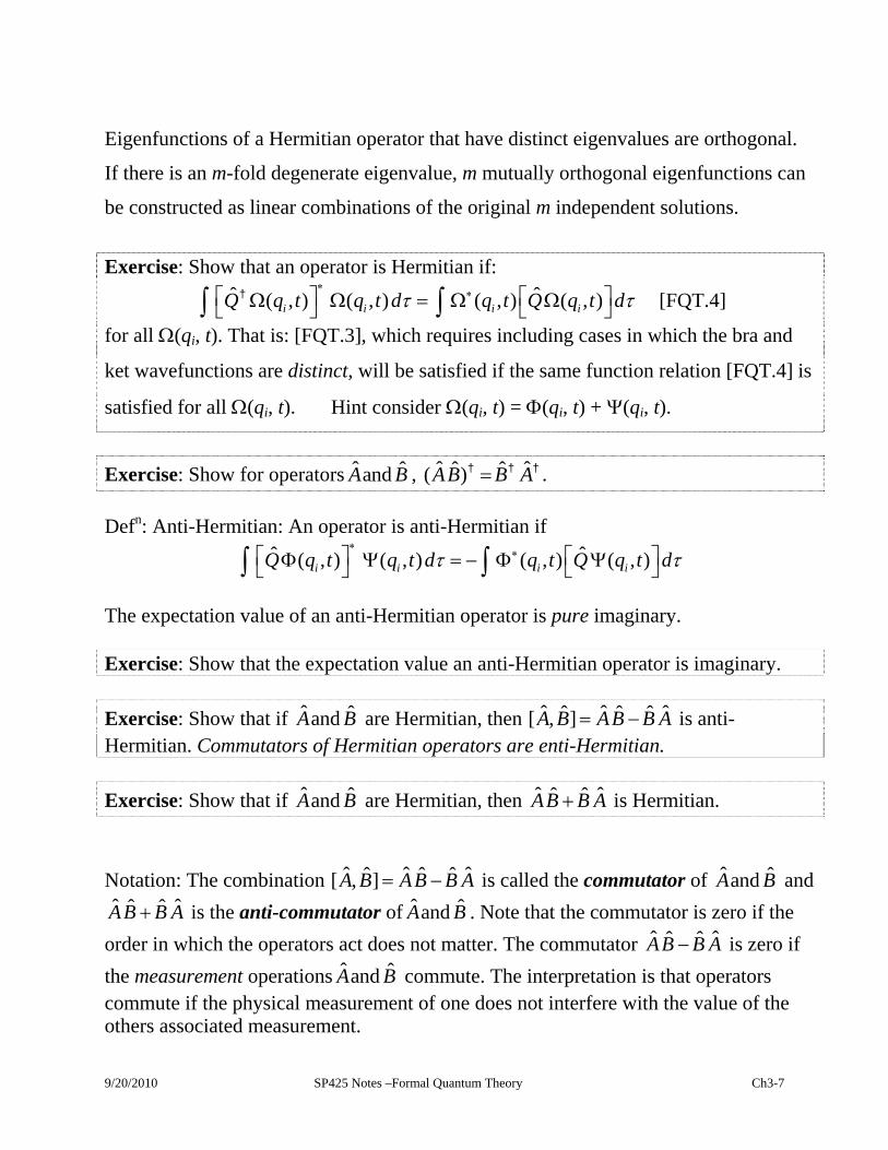
Exercise: Show that an operator is Hermitian if:


† [FQT.4]

for all (qi, t). That is: [FQT.3], which requires including cases in which the bra and

ket wavefunctions are distinct, will be satisfied if the same function relation [FQT.4] is

satisfied for all (qi, t). Hint consider (qi, t) = (qi, t) + (qi, t).

Exercise: Show for operators ˆ ândA B , ˆ ˆˆ ˆ( )AB B A† † † .

Defn: Anti-Hermitian: An operator is anti-Hermitian if


The expectation value of an anti-Hermitian operator is pure imaginary. Exercise: Show that the expectation value an anti-Hermitian operator is imaginary.

Exercise: Show that if ˆ ândA B are Hermitian, then ˆ ˆˆ ˆ ˆ[ , ] Â B AB B A is anti-Hermitian. Commutators of Hermitian operators are enti-Hermitian.

Exercise: Show that if ˆ ândA B are Hermitian, then ˆ ˆ ˆ ÂB B A is Hermitian.

Notation: The combination ˆ ˆˆ ˆ ˆ[ , ] Â B AB B A is called the commutator of ˆ ândA B and ˆ ˆ ˆ ÂB B A is the anti-commutator of ˆ ândA B . Note that the commutator is zero if the

order in which the operators act does not matter. The commutator ˆ ˆ ˆÂB B A is zero if

the measurement operations ˆ ândA B commute. The interpretation is that operators commute if the physical measurement of one does not interfere with the value of the others associated measurement.


Exercise: The commutator of the operators for two observables is formed. Will its expectation values be real or imaginary? Give an example to support your claim.

An operator can be represented by a matrix once an orthonormal basis has been

chosen for the space (problem). For the basis set { … , |n, … }, the element Qmn is

Q

ˆm nQ . Qmn is a matrix element of in the basis set { … , |n, … }

representation. (The explicit form of the matrix depends on the choice of basis.)

Q

Exercise: Show that a Hermitian operator is represented by a Hermitian matrix. A

matrix is Hermitian if it is equal to the complex conjugate of its transpose.

Postulate O1: Every Hermitian operator has a complete set of eigenfunctions that can

be used as a basis set for the full space of wavefunctions.

Postulate O2: One can find a complete basis set of functions that are simultaneous

eigenfunctions of several Hermitian operators as long as those operators commute with

one another. This result cannot be achieved if the operators fail to commute.

In the case that the operators that represent two observables do not

commute, the observables are called incompatible which means that a

measurement or observation of one disturbs the value of the other.

Postulate O3: Every problem has a maximal (largest) set of commuting Hermitian

operators. The simultaneous eigenfunctions of the operators provide a basis for the

general problem, and the eigenvalues can be used to label the states in the basis.


Postulate O4: Operators are constructed from the representation of the quantity in

Hamilton’s version of classical mechanics in which dynamical variables Q(qi, pi, t) are

natural functions of the generalized coordinates qi, the conjugate momenta (as defined

using the lagrangian: i i

Lqp ) and time. The operators are formed by replacing pk, the

momentum conjugate to qk, by -i

/qk

. (Note: This procedure is for the coordinate

space representation.)

Q(qi, pi, t) ˆ ( , , )i iqQ q i t [FQT.5]

In a case that a product of n variables is replaced, the average of the n! orderings of the

variables A and B (which are individually Hermitian) is to be substituted.

ˆ ˆˆ ˆ½ ; ½ ( ) ( ) ; ...x x xAB AB BA x p x i i x [FQT.6]

Postulate O5: Schrödinger’s equation: The hamiltonian is the time-development

operator. In most cases, it also represents the energy of the system.

ˆ ( , ) ( , )tH x t i x t

In other words, there are two operators for energy, the classical hamiltonian

transformed in accordance with Postulate O4 and i t.

This postulate leads to the expression for the time development of an expectation value:

ˆˆ ˆ[ , ] Qd itdt Q Q H

which has such embodiments as:

xd V d

xdt dtp p V

Ehrenfest's theorem States that the expectation values in quantum mechanics obey the classical

equations of motion. One notes the similar form of this theorem and Louiville's theorem from

Hamiltonian mechanics,


{ , }dQ Q

Q Hdt t

which involves the Poisson bracket{Q,H} instead of a commutator. It describes the time

development of a general dynamical variable Q. In fact, it is a rule of thumb that a theorem in

quantum mechanics which contains a commutator can be turned into a theorem in classical

mechanics by changing the commutator into a Poisson bracket and multiplying by i.

Postulate O6: A precise measurement of a dynamical variable can only return an

eigenvalue of the operator for the quantity. Making such a precise measurement at time

to collapses the state in to a state that is a linear combination of the eigenstates of that

operator that have the measured eigenvalue. (The relative amplitudes and relative

phases between the degenerate eigenstates that are consistent with the measured value

are unchanged as the result of a good, precise measurement.) If the same measurement

is repeated immediately, the result will be the same eigenvalue. The collapsed

wavefunction time develops as dictated by SE after time to so a measurement repeated

after some delay need not return the same eigenvalue.

Collapse example: Consider the position of a particle. Prior to the measurement, there

is an associated probability distribution for the position of the particle. A precise

measurement returning xo actually places the particle at that point. That is it collapses

the wavefunction to (x – xo), the eigenfunction of position corresponding to the

measured position value.


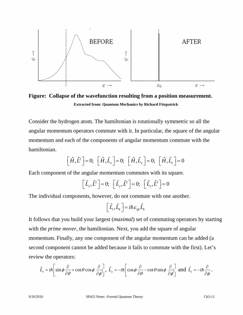
Figure: Collapse of the wavefunction resulting from a position measurement.

Extracted from: Quantum Mechanics by Richard Fitzpatrick

Consider the hydrogen atom. The hamiltonian is rotationally symmetric so all the

angular momentum operators commute with it. In particular, the square of the angular

momentum and each of the components of angular momentum commute with the

hamiltonian.

2ˆ ˆ ˆ ˆ ˆ ˆ ˆ ˆ, 0; , 0; , 0; ,x yH L H L H L H L 0z

2

Each component of the angular momentum commutes with its square.

2 2ˆ ˆ ˆ ˆ ˆ ˆ, 0; , 0; , 0x y zL L L L L L

The individual components, however, do not commute with one another.

ˆ ˆ ˆ,i k ijk kL L i L

It follows that you build your largest (maximal) set of commuting operators by starting

with the prime mover, the hamiltonian. Next, you add the square of angular

momentum. Finally, any one component of the angular momentum can be added (a

second component cannot be added because it fails to commute with the first). Let’s

review the operators:

ˆ sin cot cosxL i

, ˆ cos cot sinyL i

and ˆ

zL i

.


The z component has the simplest operator and the simplest set of eigenfunctions; let

us choose Lz as the final member of the set of commuting operators.

The maximal set: 2ˆ ˆ ˆ, , zH L L for problems with spherically symmetric potentials.

Exercise: Consider a hydrogen atom eigenfunction nlm. Relate the subscripts of the

wavefunctions to eigenvalues of each of the operators: 2ˆ ˆ ˆ, , zH L L .

Determinate State: If an ensemble of systems is prepared according to the recipe

provided by a state, and measurements on the systems in that ensemble all return

exactly the same value for an observable then that state is an eigenstate of the operator

for that observable with eigenvalue equal to the value measured.

Exercise: In the discussion of a determinate state, an ensemble of systems prepared

according to the same recipe (in the same state) was considered rather than repeating

examining the same state. Why is it important that one measurement by made on each

member of the ensemble rather than just repeating the measurement on the same

system?

Operator Example Lz: Consider the z component of angular momentum. With

standard conventions, this momentum corresponds to rotation about the z axis which

coincides with the spherical coordinate polar axis. Rotations about the polar axis

involve only . Following the prescription, the operator for the component of

momentum conjugate to qk is -i

/qk

. In this case Lz = p, so p i . This

example stretches our replacement procedure. The operator for Lz is to be developed

more carefully in the next chapter.


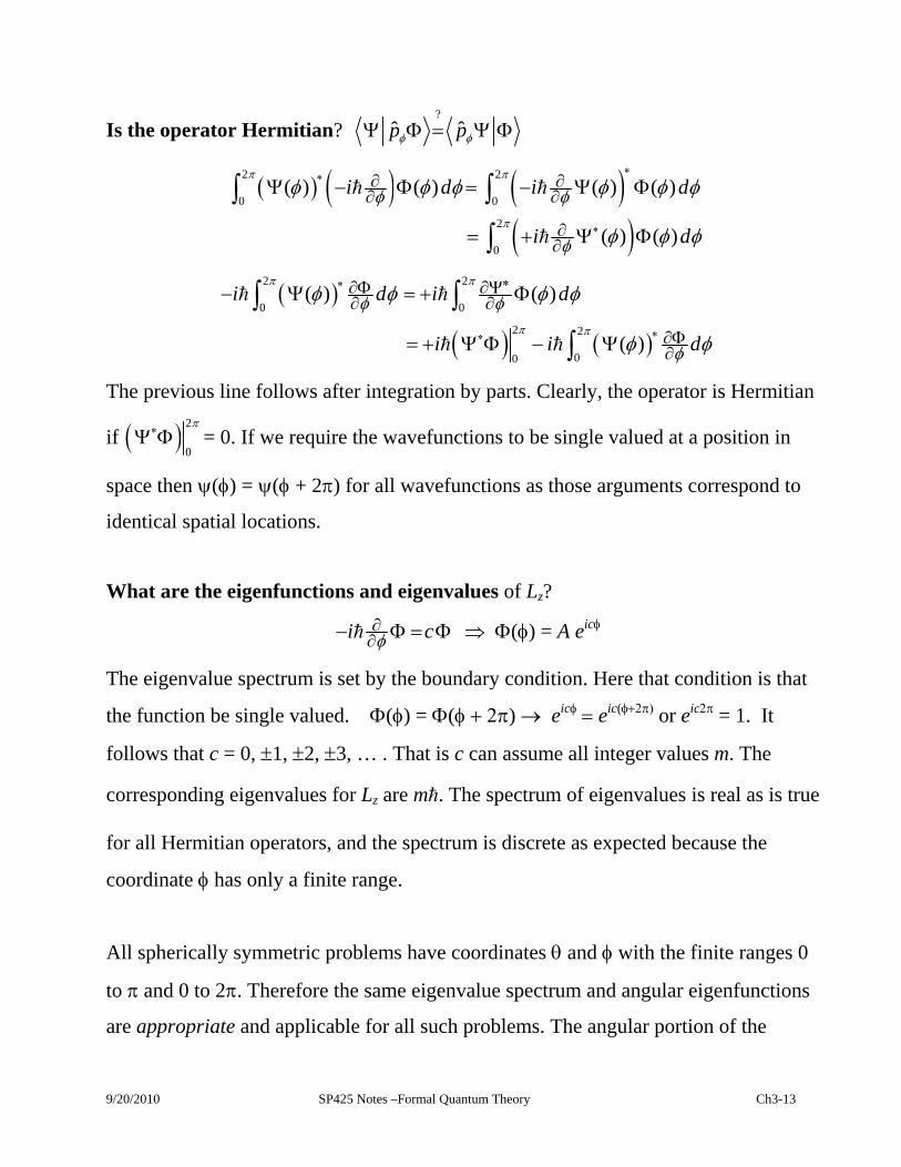
Is the operator Hermitian? ?

ˆ ˆp p

2 2

0 0

2

0

( ) ( ) ( ) ( )

( ) ( )

i d i

i d

d

2 2

0 0

2 2

00

( ) ( )

( )

i d i d

i i

d

The previous line follows after integration by parts. Clearly, the operator is Hermitian

if 2

0

= 0. If we require the wavefunctions to be single valued at a position in

space then () = ( + 2) for all wavefunctions as those arguments correspond to

identical spatial locations.

What are the eigenfunctions and eigenvalues of Lz?

i c () = A eic

The eigenvalue spectrum is set by the boundary condition. Here that condition is that

the function be single valued. () = () eiceic( or eic= 1. It

follows that c = 0, 1, 2, 3, … . That is c can assume all integer values m. The

corresponding eigenvalues for Lz are m. The spectrum of eigenvalues is real as is true

for all Hermitian operators, and the spectrum is discrete as expected because the

coordinate has only a finite range.

All spherically symmetric problems have coordinates and with the finite ranges 0

to and 0 to 2. Therefore the same eigenvalue spectrum and angular eigenfunctions

are appropriate and applicable for all such problems. The angular portion of the


eigenfunctions is one of the Ym(,) which have eigenvalues of ( + 1) 2 for the

square of the angular momentum and m for the z component of angular momentum.

Are there Lz eigenfunctions with degenerate eigenvalues? No. The differential

equation i c is first order and so has only one independent solution for each

value of c = m.

Exercise: Consider the operator 22

and repeat the processes applied to Lz above.

Compare the situations for each question.

The Momentum Representation: One could use the eigenfunctions of momentum as

the basis for an alternative representation of quantum states.

1

ˆ ( , )i px

p

t

xp i x t Aef

Not that the Planck hypothesis identifies these functions as eigenfunctions of

magnitude of momentum, and the probability current formula adds the direction.

Focusing on the spatial part, the functions are normalized with respect to p.

22| | 2 ( )p x pxi i dpA e e A p p

Dirac Orthonormal

The Dirac normalization sets |A| = (2)-½ and ( )p pf f p p .

Expanding (x) in this basis, (x) = 1

( )2

pxi dpp e

where the twiddle notation

reflects the near identity of the representation and the standard Fourier transform.


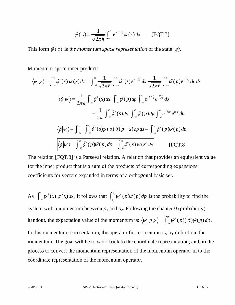
1( ) ( )

2

pxi dxp e x

[FQT.7]

This form ( )p is the momentum space representation of the state |.

Momentum-space inner product:

1 1

( ) ( ) ( ) ( )2 2

pxsxi idx ds dp dxx x s e p e

1( ) ( )

21

( ) ( )2

pxsxi i

isu ipu

ds dp

ds dp

s p e e dx

s p e e

du

( ) ( ) ( ) ( ) ( )dp dss p p s p p d

p

( ) ( ) ( ) ( )dxp p dp x x

[FQT.8]

The relation [FQT.8] is a Parseval relation. A relation that provides an equivalent value

for the inner product that is a sum of the products of corresponding expansions

coefficients for vectors expanded in terms of a orthogonal basis set.

As ( ) ( )dxx x

, it follows that 2

1

( ) ( )p

pp p dp is the probability to find the

system with a momentum between p1 and p2. Following the chapter 0 (probability)

handout, the expectation value of the momentum is: ˆ( ) ( )p p p p dp

.

In this momentum representation, the operator for momentum is, by definition, the

momentum. The goal will be to work back to the coordinate representation, and, in the

process to convert the momentum representation of the momentum operator in to the

coordinate representation of the momentum operator.


Review: (x) = 1

( )2

pxi dpp e

1

( ) ( )2

pxi dxp e x

( ) ( )

1( ) ( )

2

pxpxi idx dx

p p p p p dp

x e p x e

dp

Next, integrate over x by parts. The surface terms will be represented by 0 as the do

vanish.

1( )

2

1( )

2

px

px px

i

i

pxi

pi

i

ex

x

dx dx

dx dx

x e p

x e e dpi

dp

( )1

2( ) ( )p x xi

xdxdx x x e dpi

The final factor in parentheses is (x-x).

( ) ( ) ( )xdx dx x x x x dxdxi

ˆ ˆ( ) ( ) ( ) ( )xp p p p p dp x x dxi

The result identifies the coordinate representation of the operator for momentum.

ˆ x xp i [FQT.9]

If more dimensions had been involved, the integration by parts would have associated

the x component of momentum with the x partial derivative and so on.

p i [FQT.10]

OPERATOR x p ˆkq ˆ kp

COORDINATE REPRESENTATION x i x

qk kqi

MOMENTUM REPRESENTATION i p

p

kpi pk


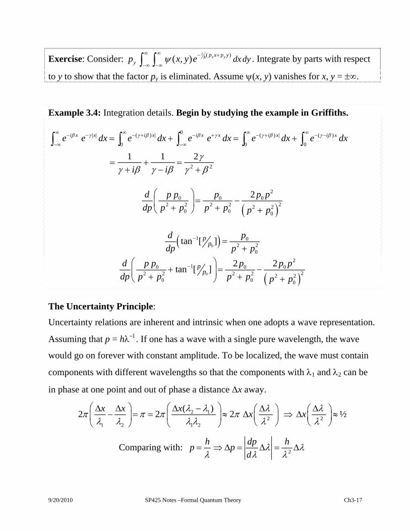
Exercise: Consider: ( )( , ) x yi p x p y

y dx dyp x y e

. Integrate by parts with respect

to y to show that the factor py is eliminated. Assume (x, y) vanishes for x, y = .

Example 3.4: Integration details. Begin by studying the example in Griffiths.

0| | ( ) | ( ) | ( )

0 0

2 2

1 1 2

i x x i x i x x i x i xe e dx e dx e e dx e dx e dx

i i

0

2

0 0 022 2 2 2 2 2

0 0 0

2d p p p p p

dp p p p p p p

0

1 02 2

0

tan [ ]pp

d p

dp p p

0

210 0

22 2 2 2 2 20 0 0

2 2tan [ ]p

pd p p p p p

dp p p p p0

p p

The Uncertainty Principle:

Uncertainty relations are inherent and intrinsic when one adopts a wave representation.

Assuming that p = h. If one has a wave with a single pure wavelength, the wave

would go on forever with constant amplitude. To be localized, the wave must contain

components with different wavelengths so that the components with 1 and 2 can be

in phase at one point and out of phase a distance x away.

2 12

1 2 1 2

( )2 2 2

x x xx

2

½x

Comparing with: 2

h dp hp p

d


2½x

2hx p [FQT.11]

To arrive at the precise uncertainty limit, one needs a precise definition of uncertainty

and a precise argument based on that definition. The immediate point is that

uncertainty is inherent in any wave representation.

REVIEW: The Hermitian conjugate of an operator is represented by the symbol Q

Q † and it is defined such that:


† [FQT.12]

for any two functions (qi,t) and (qi,t) that are permissible wavefunctions for the

problem. An operator is Hermitian if:

ˆ ˆ( , ) ( , ) ( , ) ( , ) ; ˆ î i i iQ q t q t d q t Q q t d Q Q

†

. An operator is anti-Hermitian if:

ˆ ˆ( , ) ( , ) ( , ) ( , ) ; ˆ î i i iQ q t q t d q t Q q t d Q Q

†

If A and B are Hermitian operators, then their anti-commutator ˆ ˆˆ ÂB BA is

Hermitian and their commutator ˆ ˆ ˆ ÂB BA is anti-Hermitian. Hermitian operators have

real expectation values, and anti- Hermitian operators have pure imaginary

expectation values.

The General Uncertainty Relation:

The uncertainty product for two observables is related to the commutator of their

operators. Consider two Hermitian operators A and B. Each of those operators has real

expectation values. The commutator of A and B is anti-Hermitian and has imaginary

expectation values.


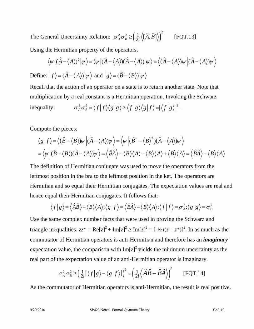
The General Uncertainty Relation: 22 2 1

2ˆ ˆ[ , ]A B i A B [FQT.13]

Using the Hermitian property of the operators,

2ˆ ˆ ˆ ˆ ˆ( ) ( )( ) ( ) ( )A A A A A A A A A A

Define: ˆ( )f A A and ˆ( )g B B

Recall that the action of an operator on a state is to return another state. Note that

multiplication by a real constant is a Hermitian operation. Invoking the Schwarz

inequality: 2 2 2| |A B f f g g f g g f f g .

Compute the pieces:

ˆ ˆˆ ˆ( ) ( ) ( )( )

ˆ ˆ ˆˆ ˆ ˆ( )( )

g f B B A A B B A A

B B A A BA B A B A B A BA B A

††

The definition of Hermitian conjugate was used to move the operators from the

leftmost position in the bra to the leftmost position in the ket. The operators are

Hermitian and so equal their Hermitian conjugates. The expectation values are real and

hence equal their Hermitian conjugates. It follows that:

2 2ˆ ˆˆ ˆ; ; ;A BAB B A BA B Af g g f f f g g

Use the same complex number facts that were used in proving the Schwarz and

triangle inequalities. zz* = Re[z]2 + Im[z]2 Im[z]2 = [-½ i(z – z*)]2. In as much as the

commutator of Hermitian operators is anti-Hermitian and therefore has an imaginary

expectation value, the comparison with Im[z]2 yields the minimum uncertainty as the

real part of the expectation value of an anti-Hermitian operator is imaginary.

222 2 1 1

2 2ˆ ˆˆ ˆ[ ]A B i if g g f AB BA [FQT.14]

As the commutator of Hermitian operators is anti-Hermitian, the result is real positive.


The standard example is 2 22 2 21 1

2 2 4ˆ ˆ ˆ ˆ[ , ] [ , ] ( )x p i ix p i x p i

2x p [FQT.15]

The Minimum Uncertainty Wave Packet:

Review the Schwarz inequality: f f g g f g g f . What is the condition for

equality? Treat |f and |gas an initial spanning set and attack with Gramm-Schmidt

sans normalization.

Gram-Schmidt Term

where 0f g f g

g f g f c f h f hf f f f

Whenever you have two vectors, |f and |g the second can be decomposed into c|f a

multiple of the first, plus a vector |h that is orthogonal to the first.

2

22

f f g g f f c f h c f h f f c f f h h

f g g f c f f c f f c f f

Clearly, the equality only holds if |h = |ZERO; that is: if |g is just a multiple of |f .

The minimum uncertainty packet corresponds to the case in which there is equality.

Define: ˆ( )f x x and ˆ( )g p p . Recall that the action of an operator

on a state is to return another state. Note that multiplication by a real constant is a

Hermitian operation. Invoke the Schwarz inequality:

2 2 2| |A B f f g g f g g f f g .

Look for the minimum uncertainty which requires that |g = c |f . Recall [FQT.14].

2 222 2 1 1 1

2 2 2 0ˆ ˆ ˆˆ ˆ ˆ,[ ] [ ]A B i i if g g f AB BA A B


We kept only the imaginary part of f|g when the relation was derived so equality

requires that |g is a purely imaginary multiple of |f |g = i a |f where a is real

f g f i a f i a f f is pure imaginary only if a is real.

|g = i a |f 2ˆ ˆ( ) ( ) ( )i xp p p i x x

The constant a was set to 2. Using the notations: po = p and xo = x

20 ( )i x p i x x0

[FQT.16]

This equation has the familiar solution,2

0 / ½ ( )ip x a x xAe e 0 , a Gaussian wave

packet. As a first order DE has only one independent solution, we have the answer for

one dimension.

Exercise: Replace | by (x) in equation [FQT.16] to get the coordinate

representation of the problem. Divide the equation by (x) and then take the anti-

derivatives term by term. Don’t forget to include an integration constant. Find (x).

Compare your result with .2

0 0/ ½ ( )ip x a x xAe e

Energy-Time Uncertainty: Uncertainty relations are inherent in a wave

representation. Assuming that E = , one counts cycles to determine the frequency. If

one counts n cycle completions in a time T, then the frequency is determined to one

part out of n. The frequency is n/T so it uncertainty is 1/T. The product of the

observation time and the uncertainty is T (1/T) 1. Shuffling symbols,

t (f) 1 t (hf) h t (E) h.

To arrive at the strict uncertainty limit, one needs a precise definition of uncertainty

and a precise argument based on that definition. The immediate point is that

uncertainty is inherent in a wave representation.


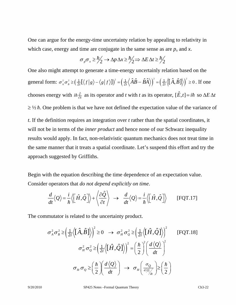
One can argue for the energy-time uncertainty relation by appealing to relativity in

which case, energy and time are conjugate in the same sense as are px and x.

2 2p x p x E t 2

One also might attempt to generate a time-energy uncertainly relation based on the

general form: 2 222 2 1 1 12 2 2 0ˆ ˆ ˆˆ ˆ ˆ,[ ] [ ]

A B i i if g g f AB BA A B . If one

chooses energy with ti as its operator and t with t as its operator, ˆ[ , ]E t i so E t

½ . One problem is that we have not defined the expectation value of the variance of

t. If the definition requires an integration over t rather than the spatial coordinates, it

will not be in terms of the inner product and hence none of our Schwarz inequality

results would apply. In fact, non-relativistic quantum mechanics does not treat time in

the same manner that it treats a spatial coordinate. Let’s suspend this effort and try the

approach suggested by Griffiths.

Begin with the equation describing the time dependence of an expectation value.

Consider operators that do not depend explicitly on time.

ˆˆ ˆˆ ˆ, ,

d i Q d iQ H Q Q H Q

dt t dt

[FQT.17]

The commutator is related to the uncertainty product.

22 2 1

2 0ˆ ˆ,[ ]A B i A B 22 2 1

2ˆˆ ,[ ]H Q i H Q [FQT.18]

222

2 2 12 2

ˆˆ ,[ ]H Q id Q

dtH Q

2 2d Qdt

H Q HQd Q

dt


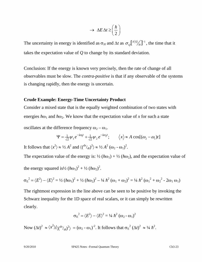
2E t

The uncertainty in energy is identified as H and t as 1[ ]d QdtQ

, the time that it

takes the expectation value of Q to change by its standard deviation.

Conclusion: If the energy is known very precisely, then the rate of change of all

observables must be slow. The contra-positive is that if any observable of the systems

is changing rapidly, then the energy is uncertain.

Crude Example: Energy-Time Uncertainty Product

Consider a mixed state that is the equally weighted combination of two states with

energies 1 and 2. We know that the expectation value of x for such a state

oscillates at the difference frequency 2 – 1.

1 21 2 2

1 12 2

; cos[(i t i te e x A 1) ]t

It follows that x2 ½ A2 and (dx/dt)2 ½ A2 (2 - 1)

2.

The expectation value of the energy is: ½ (1) + ½ (2), and the expectation value of

the energy squared is½ (1)2 + ½ (2)

2.

E2E2 = ½ (1)

2 + ½ (2)2 – ¼ 2 (1 + 2)

2 = ¼ 2 (12 + 2

2 - 211)

The rightmost expression in the line above can be seen to be positive by invoking the

Schwarz inequality for the 1D space of real scalars, or it can simply be rewritten

clearly.

E2E2 = ¼ 2 (2

- 1)2

Now (t)2 x2(dx/dt)2(2 - 1)

-2. It follows that (t)2 ¼ 2.


The point is that, if the energy is precisely defined, is small, then t must be large

so expectation values change only very slowly.

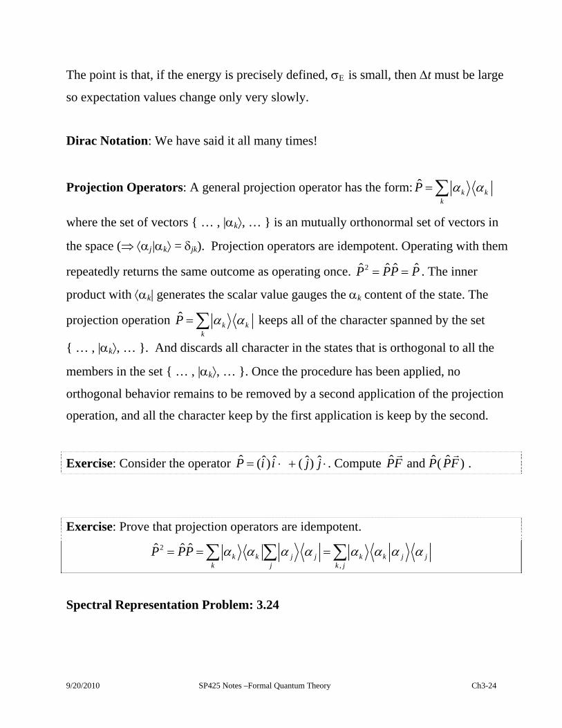
Dirac Notation: We have said it all many times!

Projection Operators: A general projection operator has the form: ˆk k

k

P

where the set of vectors { … , |k, … } is an mutually orthonormal set of vectors in

the space (j|k = jk). Projection operators are idempotent. Operating with them

repeatedly returns the same outcome as operating once. 2ˆ ˆ ˆP PP P . The inner

product with k| generates the scalar value gauges the k content of the state. The

projection operation ˆk k

k

P keeps all of the character spanned by the set

{ … , |k, … }. And discards all character in the states that is orthogonal to all the

members in the set { … , |k, … }. Once the procedure has been applied, no

orthogonal behavior remains to be removed by a second application of the projection

operation, and all the character keep by the first application is keep by the second.

Exercise: Consider the operator ˆ ˆ ˆ ˆ ˆ( ) ( )P i i j j . Compute .ˆ ˆ ˆand ( )PF P PF

Exercise: Prove that projection operators are idempotent.

2

,

ˆ ˆ ˆk k j j k k j j

k j k j

P PP

Spectral Representation Problem: 3.24


Tools of the Trade

Time development of an arbitrary wavefunction:

General Time Dependence: Eigenfunctions of the hamiltonian play a

special role because they have a separable time dependence.

Eigenvalue equation: ˆ ( , ) ( , )n n nH x t E x t

1where( , ) ( ) nn n n

i tnx t x e E and ˆ ( , ) ( , )n n nH x t E x t

Any function can be expanded in terms of the n(x) at a time to.

0 0( , ) ( ) ( )n nall n

x t a t x

The wave function at any time is 00

( )( , ) ( ) ( ) nn n

all n

i t tx t a t x e .

Consider the matrix in Griffiths example 3.8. In the basis set {|1, |2}, the states and

hamiltonian have the representations:

1 01 ; 2 ;

0 1

h gH

g h

.

In the matrix, g and h are real constants (in general, the matrix must be Hermitian).

Each matrix element is computed as Hmn = m|H|n. The time dependence of an

arbitrary state is found by finding the eigenvectors of the hamiltonian that have the

simple eint

time dependences. The arbitrary state is expanded in terms of the

eigenvectors at the initial time to.

1 21 2 1 20

1 2 1 2

( ) ( )( ) ; ( ) o oi t t i t ta a a at c d t c d

b b b be e

The time dependence follows from that for the eigenvectors.


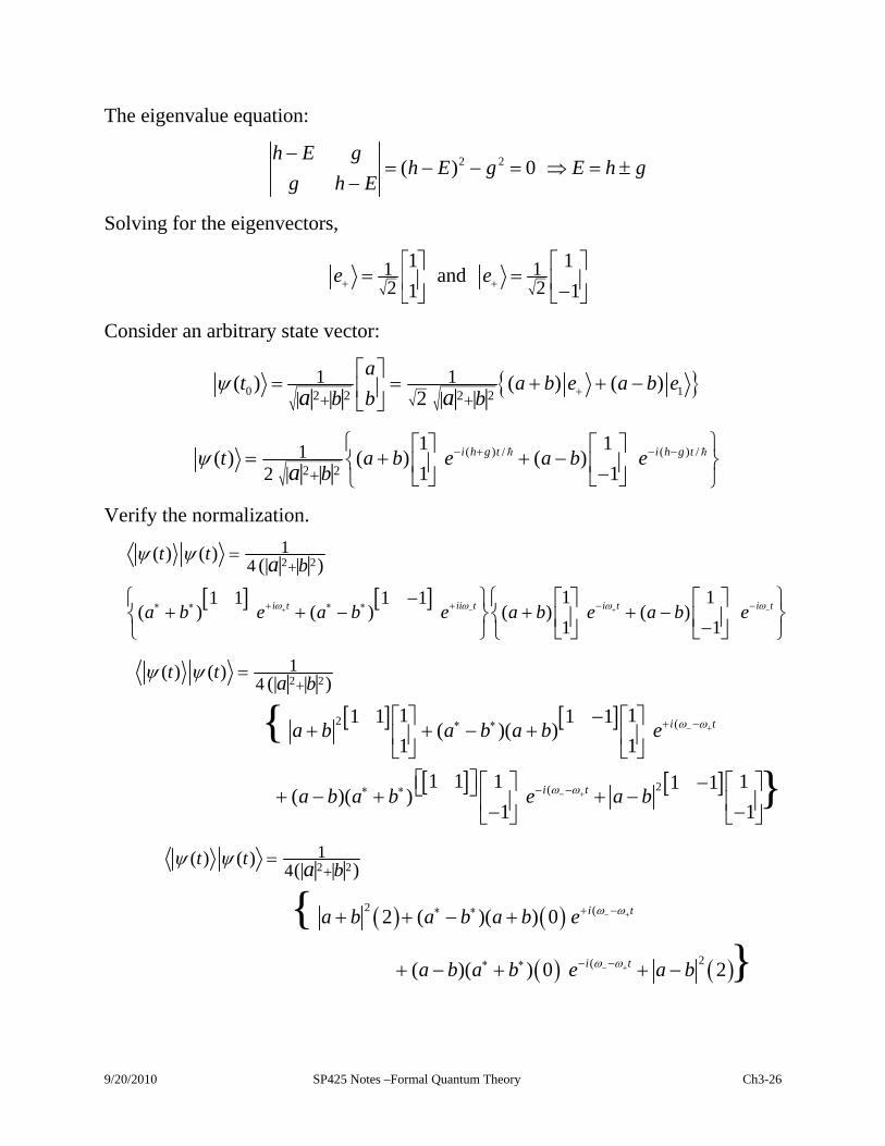
The eigenvalue equation:

2 2( ) 0h E g

h E g E h gg h E

Solving for the eigenvectors,

1 12 2

1 1and

1 1e e

Consider an arbitrary state vector:

0 12 2 2 21 1

| |( ) ( ) ( )

| 2 || | | |a

t a b ebb ba a

a b e

( ) / ( ) /

2 21

2 |

1 1( ) ( ) ( )

1 1|| |i h g t i h g tt a b e a b e

ba

Verify the normalization.

2 21

4( ) ( )

1 11 1 1 1( ) ( ) ( ) ( )

1 1

(| | )| |

i t ii t i t i t

t t

a b e a b e a b e a b e

ba

2 2

2 (

2(

14

( ) ( )(| | )

1 11 1 1 1( )( )

1 1

1 1 1 11 1( )( )

1 1

| |

{

}

i t

i t

t tb

a b a b a b e

a b a b e a b

a

2 2

2 (

2(

14

( ) ( )(| | )

2 ( )( ) 0

( )( ) 0 2

| |

{}

i t

i t

t tb

a b a b a b e

a b a b e a b

a


2 24( ) ( )

(| | )( )( ) ( )(2

| |t tb

a b a b a b a ba

)

2 22 )( ) ( )

(| |( ) (1

| |t tb

aa bb ab a b aa bb ab a ba

) 1

The state is normalized and that normalization is preserved in time.

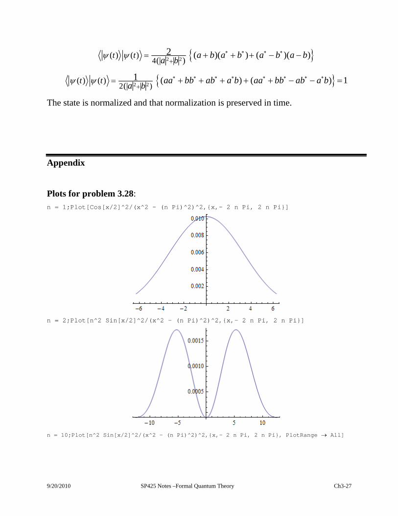
Appendix

Plots for problem 3.28: n = 1;Plot[Cos[x/2]^2/(x^2 - (n Pi)^2)^2,{x,- 2 n Pi, 2 n Pi}]

n = 2;Plot[n^2 Sin[x/2]^2/(x^2 - (n Pi)^2)^2,{x,- 2 n Pi, 2 n Pi}]

n = 10;Plot[n^2 Sin[x/2]^2/(x^2 - (n Pi)^2)^2,{x,- 2 n Pi, 2 n Pi}, PlotRange All]


n = 40;Plot[n^2 Sin[x/2]^2/(x^2 - (n Pi)^2)^2,{x,- 2 n Pi, 2 n Pi}, PlotRange All]

Notation for a matrix representation of the vector space:

A letter in outline ( ) represents an operator, a square matrix. n represents a column vector,

and n represents a row vector, the complex conjugate of the transpose of n .

n = n

t = n

†

Most physical quantities are represented by Hermitian operators. A Hermitian matrix is equal to

its Hermitian conjugate, the complex conjugate of its transpose.

( t)*

Hermitian is the complex generalization of real symmetric. Hermitian matrices, like real symmetric

matrices, have real eigenvalues, orthogonal eigenvectors for distinct eigenvalues and eigenvectors


that may be chosen to be orthogonal even in degenerate (equal eigenvalue) cases. Moreover, the

eigenvectors are to be normalized. Orthonormal is shorthand for orthogonal and normalized.

Translating between vector space Bra-Ket | | and matrix notations for N = 2.

The first step is to adopt a basis set | and | which have the canonical

representations: 1

1

0

and 2

0

1

.

a general Bra vector 1 2

j

j j jj

aa b

b

a Ket vector

** *i i i i

ii i

ta b a a

b b

†

t is the Hermitian conjugate, the complex conjugate of the transpose

inner product * *

* *ji ii j i j i

j

aa ba a b b

b

j

operator : where 11 12

21 22

O O

O O

ˆ

i j i jO O , the representation of the

operator in the chosen basis set. Hermitian ( )t.

11 12

21 22

* *ˆ ji i

i jj

aa b O OO

bO O

expectation value:

11 12

21 22

* *

* *

ˆjj j

jj j

j j jj j

j

aa b O O

bO OO

aa b

b

expectation value: 11 12

21 22

* *ˆ jj j

j jj

aa b O OO

bO O

for normalized states =1 * *i j i ja a b b

eigenvalue equation j = oj j where oj is a scalar

11 12

21 22

j j

jj j

a aO Oo

b bO O


orthonormal * *

* *ji ii j i j i j i

j

aa ba a b b

b j

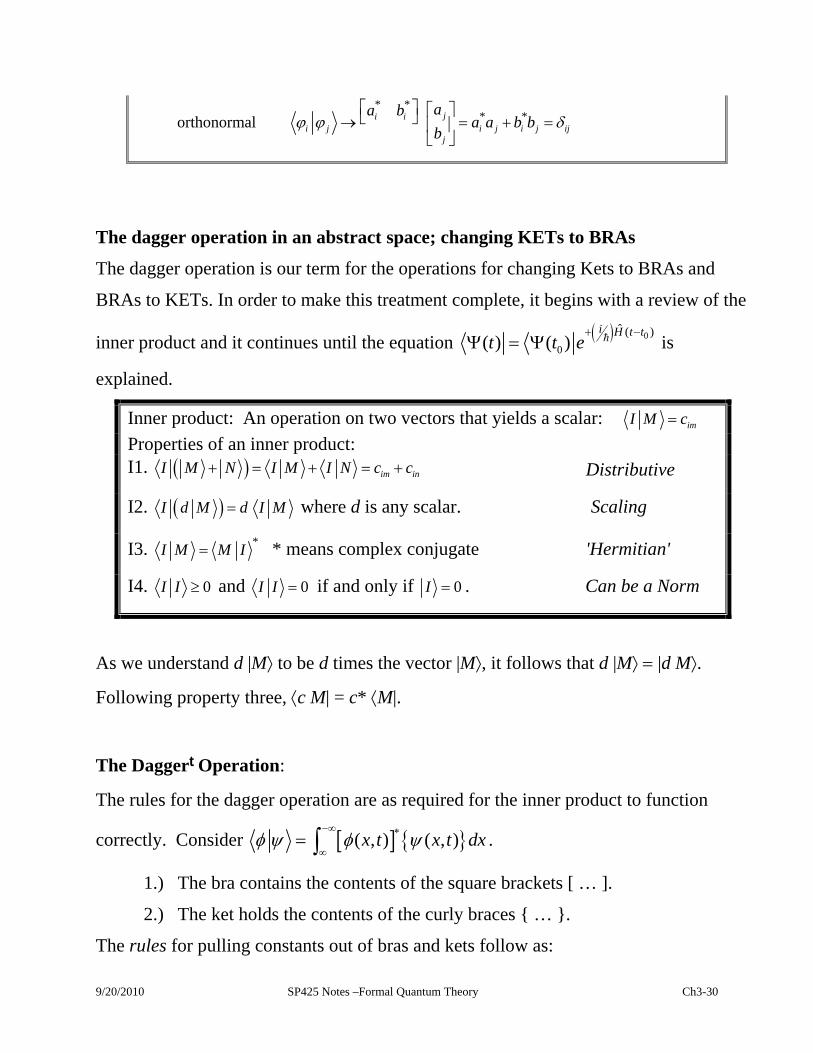
The dagger operation in an abstract space; changing KETs to BRAs

The dagger operation is our term for the operations for changing Kets to BRAs and

BRAs to KETs. In order to make this treatment complete, it begins with a review of the

inner product and it continues until the equation 0

0

ˆ (( ) ( )

i H t tt t e

)

is

explained.

Inner product: An operation on two vectors that yields a scalar: imI M c

Properties of an inner product: I1. im inI M N I M I N c c Distributive

I2. I d M d I M where d is any scalar. Scaling

I3. *I M M I * means complex conjugate 'Hermitian'

I4. 0I I and 0I I if and only if 0I . Can be a Norm

As we understand d |M to be d times the vector |M, it follows that d |M |d M.

Following property three, c M| = c* M|.

The Daggert Operation:

The rules for the dagger operation are as required for the inner product to function

correctly. Consider ( , ) ( , )x t x t

dx .

1.) The bra contains the contents of the square brackets [ … ].

2.) The ket holds the contents of the curly braces { … }.

The rules for pulling constants out of bras and kets follow as:


( , ) ( , ) ( , ) ( , )c x t c x t dx c x t x t dx c

and

( , ) * , ) * ( , ) ( , ) *c c x t x t dx c x t x t dx c

.

Apply parallel reasoning when you examine the other dagger rules.

1.) The dagger operation converts a KET vector to its corresponding (conjugate) BRA

vector. That is: M Mt .

2.) The dagger operation also converts a BRA vector to its corresponding (conjugate)

KET vector.

3.) The repeated operation is the identity which is a way to say that if the dagger

operation is performed twice, the original vector is recovered. M M M tt t .

4.) The dagger on a BRA-KET follows as ( )I M M It . The inner product of two

vectors is a scalar and *I M M I so the dagger operation acting on a scalar returns

the complex conjugate of that scalar; (d )† = d*.

5.) Dagger operation on multiplying constants: (d |M)† |d M† = d M| = d* M|.

NOTE: Dagger should appear as †

but font wars are leading to and even to a superscript t (t). †

Computers are simplifying our lives! Read †

and as †

. †

Exercise: Express ˆiO with a constant and the operator appearing in the ket.

Express ˆcO with a scalar and the operator in the bra. Rewrite ˆˆ ˆi H A p with

all the operators and multiplying constants in the ket. The dagger of ˆ /iHte is


ˆ /iHte . Express ˆ /iHte with the operator in the sandwich position. Do so first

without assuming that is Hermitian and then assuming that it is Hermitian. H

Hermitian conjugate or adjoint operator

Adjoint Operator: One rule for moving things from BRA to KET or from KET to

BRA is not enough. The adjoint of an operator is itself an operator that acts in the BRA

of an inner product to yield the same result as the original operator acting in the KET.

The adjoint of an operator is defined by its action. Q† Q

ˆ ˆQ u v u Q v u and v †

Note that there are two processes that move the operator from the KET vector to the

BRA vector: (1.) complex conjugation and (2.) switching to the adjoint.

6.) The leftmost operator in the Ket can be moved to be the leftmost operator in the Bra

if it is also conjugated.

ˆ ˆ ˆ ˆ ˆ ˆ ˆ ˆˆ ˆ ˆ ˆ ˆ ˆ ˆ ândA B C D C A B D A B C D B A C D † †

7.) ˆ ˆ Â A †

†A where the expressions must operate on a ket.

ˆ ˆ(...) (...)A A † .

This final form makes it clear that ˆ ˆ Â A †

†A is not a new rule; it is

simply a strange way to express the definition of Hermitian conjugate.

Dagger Operation Examples:

1.) The Schwarz vector: B A B A B B

A AB B B

†

B


Each Ket is changed to the corresponding Bra and vice versa. For the inner products

the same rule works, but equivalently A|B = d, a scalar so A|B† = d† = d* = B|A

according to the Hermitian property of the inner product.

2.) The Schrödinger equation:

ˆ ˆ ˆH i H i H it t

†† ††

t

Non-Hermitian operators: The notation ˆ ˆmeansQ Q .

ˆ ˆQ Q †

The symbol Q can be interpreted as the operator Q acting to the right on the

state in the Ket or its Hermitian conjugate acting to the right (only) in the Bra.

3.) ˆ ˆ( ) ( )A A A A ;

ˆ ˆ ˆ ˆ ˆ( ) ( ) ( ) ( ) ( )A A A A A A A A A A

† †† † †

Time Development (given H/t = 0): According to Taylor, if the state and all its time

derivatives are known at time to, then, at later times, the state is:

0

0 00 0

1 1! !( , ) ( ) ( , ) ( , ) ( )m m

tm m

m mm mm mt t 0x t t t x t x t

t t

ˆ ˆ( , ) ( ,0)mm

mmi

t tH i x t H x

0

0 00

ˆ ( )1!

ˆ( , ) ( , ) ( ) ( , )m

m m

m

i H t t

mi

0x t H x t t t e

x t


The development details of a companion relation are rarely presented. We are to err by

being overly detailed (perhaps a greater sin).

The companion relation: 0

0

ˆ (( , ) ( , )

i )H t tx t x t e

. The relation is a real puzzler

because the operators are rightmost, and, by default, that it is the direction in which

they operate. To decode this mess, it operation on an arbitrary ket must be examined.

Start with a much simpler problem: the time development of eigen-bras and –kets.

ˆn n n n nt tH E i i

( ) (0) (0)n

n n

Eni t i tt e e n

Recall the Schrödinger representation of the inner product.

( ) ( ) ( ) ( ) (0) (0)

[ ] (0) (0)

n m

n m

b b i t i tn m n m n ma a

bi t i tn ma

t t t t dx e e dx

e e dx

One expects that an eigen-bra has e+it as a standard time-dependence

An eigen-ket has the standard e-it time-dependence. Note: there are no operators in the

expression, just scalar values, and the En’s are real so that En† = En . Applying the

dagger operation,

( ) ( ) ( ) ( )n

n n n

E En ni t i t i tt e t e t e t

†

n

This result is exactly as expected.

We begin at the beginning with: ît H . The operators attack right.

ît H

Apply the dagger operation.

ît H


Digression: Examine the relation in the case of an eigenstate.

( ) (0)m mi tm m m m m m

i it E E t e

The next step is to move the operators out of the bra which requires that an inner

product with an arbitrary ket is assumed.

ˆ ˆt

i iH H

†

ˆt

i H

The fact that the hamiltonian is Hermitian was used as well as (-i)† = i. Removing the

arbitrary state, the operator version of the relation is:

ˆ ˆ... (...) ort ti iH H

Applying these result to the full time development operator,

0 0

0 0

ˆ ˆ( ) ( )( , ) ( , ) ( , )

i iH t t H t tx t e x t e x t

Apply the dagger operation.

0 0

0 0

ˆ ˆ( ) ( )( , ) ( , ) ( , ) [ ]

i iH t t H t tx t e x t x t e

†

0

0

ˆ ( )( , ) ( , )

i H t tx t x t e

Once again, the hamiltonian is Hermitian and time independent. As before, this result

is an operator equation, and the operators need a ket on which to act.

0 0

0 0

ˆ ˆ( ) ( )( , ) ( , ) ( , ) ... ( , ) (...)

i iH t t H t tx t x t e x t x t e

The general conclusion is that: ˆ ˆ ˆA A †

†A where the expressions must

operate on a ket ˆ ˆ(...) (...)A A † .


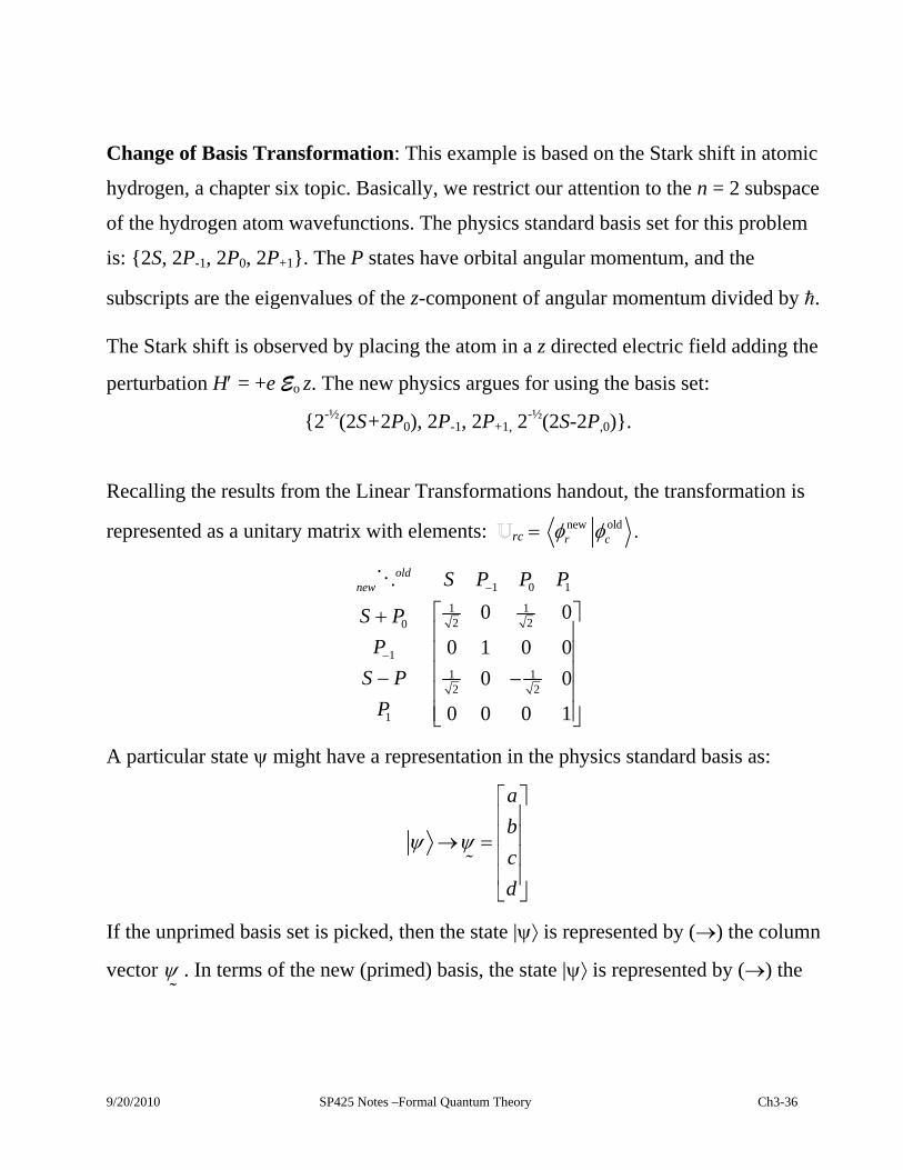
Change of Basis Transformation: This example is based on the Stark shift in atomic

hydrogen, a chapter six topic. Basically, we restrict our attention to the n = 2 subspace

of the hydrogen atom wavefunctions. The physics standard basis set for this problem

is: {2S, 2P-1, 2P0, 2P+1}. The P states have orbital angular momentum, and the

subscripts are the eigenvalues of the z-component of angular momentum divided by .

The Stark shift is observed by placing the atom in a z directed electric field adding the

perturbation H = +e Eo z. The new physics argues for using the basis set:

{2-½(2S+2P0), 2P-1, 2P+1, 2-½(2S-2P,0)}.

Recalling the results from the Linear Transformations handout, the transformation is

represented as a unitary matrix with elements: rc new oldr c

1 0 1

1 12 20

1

1 12 2

1

0 0

0 1 0 0

0 0

0 0 0 1

oldnew S P P P

S P

P

S P

P

A particular state might have a representation in the physics standard basis as:

a

b

c

d

If the unprimed basis set is picked, then the state | is represented by () the column

vector

. In terms of the new (primed) basis, the state | is represented by () the


column vector

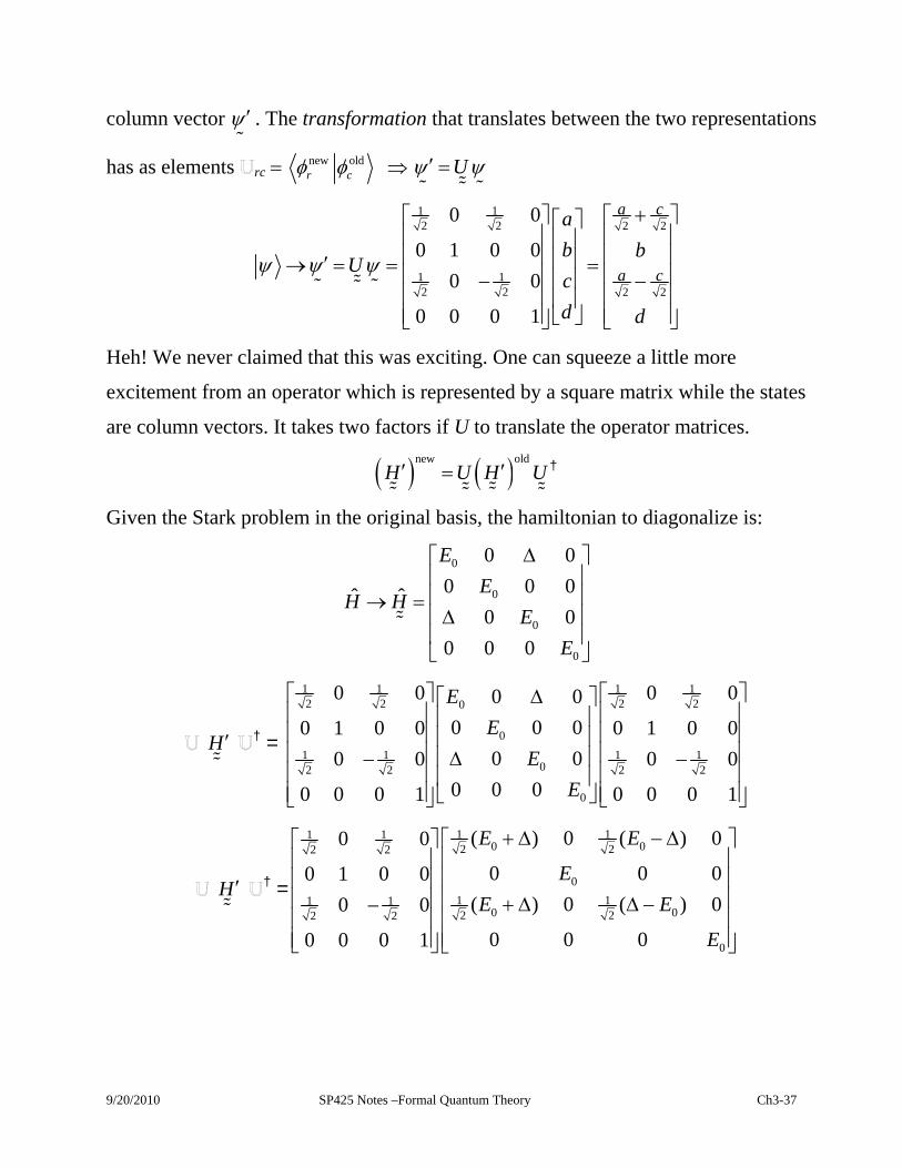
. The transformation that translates between the two representations

has as elements rc new oldr c U

1 1

0 1

0 0

2 2 2 2

1 12 2 2 2

0 0

0 0

0 0

0 1

a c

a c

a

b bU

c

d d

Heh! We never claimed that this was exciting. One can squeeze a little more

excitement from an operator which is represented by a square matrix while the states

are column vectors. It takes two factors if U to translate the operator matrices.

new old

H U H U

†

Given the Stark problem in the original basis, the hamiltonian to diagonalize is:

0

0

0

0

0 0

0 0ˆ ˆ0 0

0 0 0

E

EH H

E

0

E

H

† =

1 1 1 12 2 2 20

0

1 1 1 102 2 2 2

0

0 0 0 00 0

0 0 00 1 0 0 0 1 0 0

0 00 0 0 0

0 0 00 0 0 1 0 0 0 1

E

E

E

E

H

† =

1 11 10 02 22 2

0

1 11 10 02 22 2

0

( ) 0 ( ) 00 0

0 00 1 0 0

( ) 0 ( ) 00 0

0 0 00 0 0 1

E E

E

E E

0

E


H

†

0

0

0

0

0 0 0

0 0

0 0 0

0 0 0

E

E

E

0

E

Once the diagonal form is found, the eigenvalues can be read off the diagonal. The

values above are bursting with meaning! See chapter six.

Chemists use a basis set of wavefunctions to represent sates that might form bonds at

right angles. {2S, 2Px, 2Py, 2Pz}. The state |2Pz is identical to the physics standard

state |2P0, but it does appear at position four rather than at three in the list.

|2Pxchem = 2-½(|2P1|2P-1)phys; |2Pychem =-i 2-½(|2P1|2P-1)phys; |2Pzchem = |2P0phys

1 0 1

1 0

1

1

2 2 2 2 2 2 2 2

2 2

2 2

xx

y

zz

S P P P

S S S P S P S PS

P PP

P

P PP

1

Exercise: Find the explicit form of the transformation matrix to convert from the

physics standard basis to the chemist’s orthogonal bound set.

Chemists use a basis set for these states in which all four have equal admixtures of

each character in the physics set. The states are appropriate for representing bonds with

tetrahedral coordination. Consider the methane molecule, CH4. I have no clue what

chemists would choose for conventions, but here is a possible transformation matrix

from the physics standard basis to the tetrahedral coordinated basis.


1 0 1

½ ½ ½ ½

½ ½ ½ ½

½ ½ ½ ½

½ ½ ½ ½

a

b

c

d

S P P P

T

T

T

T

I almost guessed correctly! The transformation above actually appears in a chemistry

text, but it is to be used to transform from the previous {2S, 2Px, 2Py , 2Pz} basis. The

correct process is then to transform from the physics standard basis to the chemistry set

above and then to transform again to reach the tetrahedral bond set.

1 01 0 1

11 12 13 141 1

21 22 23 24 2 2

31 32 33 34 2 2

41 42 43 44

1 0 0 0½ ½ ½ ½0 0½ ½ ½ ½

½ ½ ½ ½ 0 0

½ ½ ½ ½ 0 0 1 0

oldnewx y z

a a

b b x

c c y

d d z

i i

S P P PS P P P S P P P

T u u u u T S

T u u u u T P

T u u u u T P

T u u u u T P

1

matrix multiply with the later action on the left

Exercise: Give the explicit form of the matrix representing transforming from the

physics basis set {2S, 2P-1, 2P0, 2P+1} to the tetrahedral coordination basis set used by

the chemists.


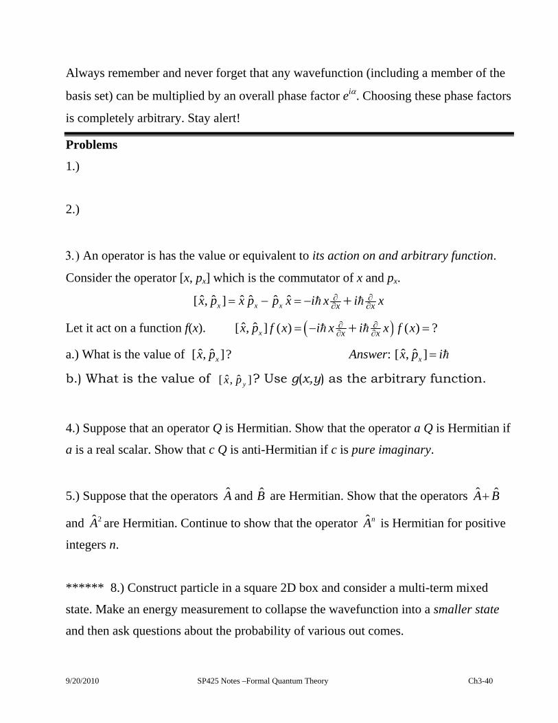
Always remember and never forget that any wavefunction (including a member of the

basis set) can be multiplied by an overall phase factor ei. Choosing these phase factors

is completely arbitrary. Stay alert!

Problems

1.)

2.)

An operator is has the value or equivalent to its action on and arbitrary function.

Consider the operator [x, px] which is the commutator of x and px.

ˆ ˆ ˆ ˆ ˆ ˆ[ , ]x x x x xx p x p p x i x i x

Let it act on a function f(x). ˆ ˆ[ , ] ( ) ( ) ?x x xx p f x i x i x f x

a.) What is the value of ˆ ˆ[ , ]xx p ? Answer: ˆ ˆ[ , ]xx p i

b.) What is the value of ˆ ˆ[ , ]yx p ? Use g(x,y) as the arbitrary function.

4.) Suppose that an operator Q is Hermitian. Show that the operator a Q is Hermitian if

a is a real scalar. Show that c Q is anti-Hermitian if c is pure imaginary.

5.) Suppose that the operators ˆ ˆandA B are Hermitian. Show that the operators ˆ ˆA B

and 2A are Hermitian. Continue to show that the operator ˆ nA is Hermitian for positive

integers n.

****** 8.) Construct particle in a square 2D box and consider a multi-term mixed

state. Make an energy measurement to collapse the wavefunction into a smaller state

and then ask questions about the probability of various out comes.


8. An operator is has the value or equivalent to its action on and arbitrary function. a.)

Consider the operator [x, px] which is the commutator of x and px.

ˆ ˆ ˆ ˆ ˆ ˆ[ , ]x x x x xx p x p p x i x i x

Let it act on a function f(x). ˆ ˆ[ , ] ( ) ( ) ?x x xx p f x i x i x f x

What is the value of ˆ ˆ[ , ]xx p ? Answer: ˆ ˆ[ , ]xx p i

b.) Consider the operator [x, 2

2x ] which is the commutator of x and

2

2x .

Let it act on a function f(x). [x, 2

2x ] f(x) = ?

c.) Consider the operator [x, H ] which is the commutator of x and H where 2

22ˆ ( )m xH V x

. Let it act on a function f(x). [x, H ] f(x) = ?

9. A Hermitian operator has a complete set of eigenfunctions. Q ˆn nQ q n .

a.) Show that the expectation value of in the eigenstate m is qm. Q

b.) Write down the defining condition for the operator to be Hermitian. Q

c.) Show that the eigenvalues of are real. Q

d.) Show that the expectation value of in a mixed state Q1

( , ) ( , )m mm

x t a x t

is

2

1

ˆm m

m

Q a

q .

Conclude that Hermitian operators have real eigenvalues and expectation values. These

properties make them candidates to represent observables.

10.) A particle is in a 2D infinite well: (0 x a; 0 y a). The eigenfunctions are:


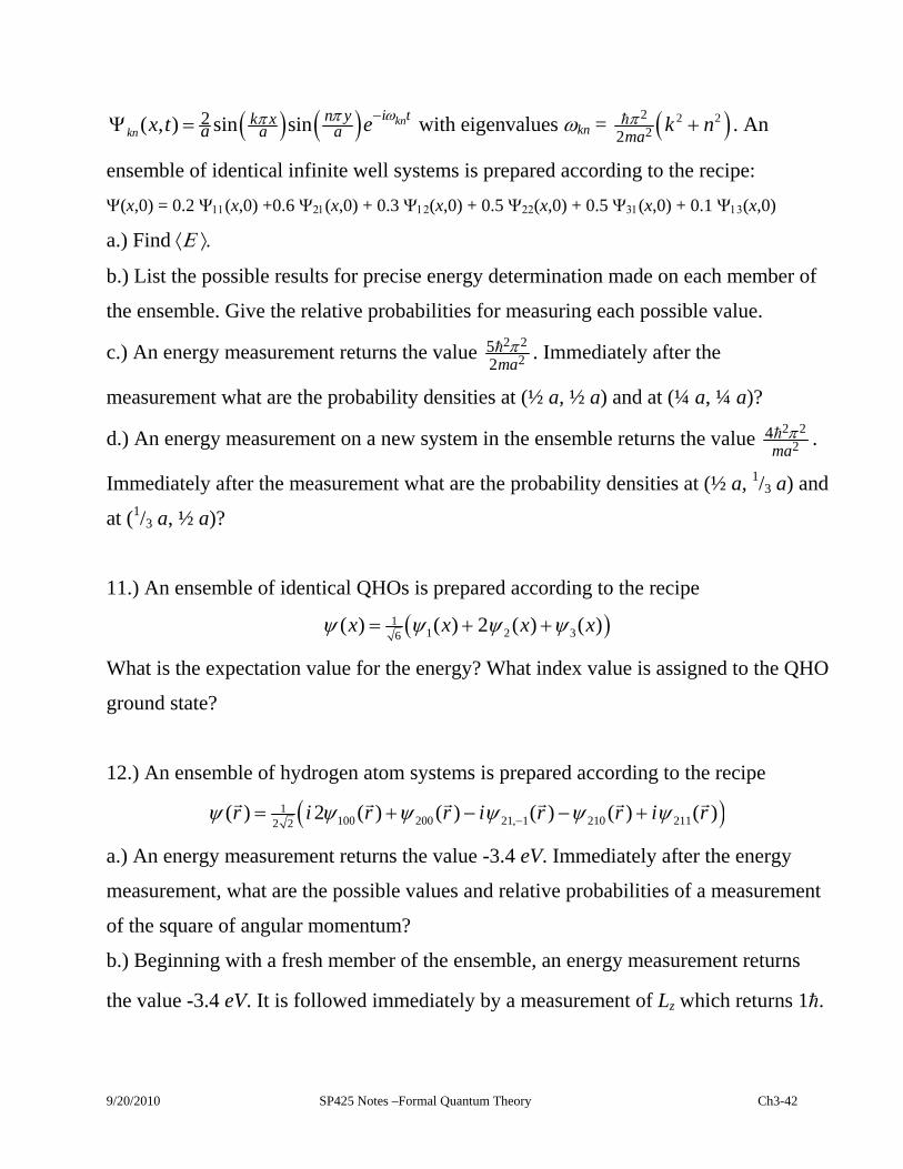
2( , ) sin sin knkn

in yk xa aax t e t with eigenvalues kn = 2 22

22mak n . An

ensemble of identical infinite well systems is prepared according to the recipe:

(x,0) = 0.2 (x,0) +0.6 (x,0) + 0.3 (x,0) + 0.5 (x,0) + 0.5 (x,0) + 0.1 (x,0)

a.) Find

b.) List the possible results for precise energy determination made on each member of

the ensemble. Give the relative probabilities for measuring each possible value.

c.) An energy measurement returns the value 2 2

252ma

. Immediately after the

measurement what are the probability densities at (½ a, ½ a) and at (¼ a, ¼ a)?

d.) An energy measurement on a new system in the ensemble returns the value 2 2

24ma .

Immediately after the measurement what are the probability densities at (½ a, 1/3 a) and

at (1/3 a, ½ a)?

11.) An ensemble of identical QHOs is prepared according to the recipe

11 2 36

( ) ( ) 2 ( ) ( )x x x x

What is the expectation value for the energy? What index value is assigned to the QHO

ground state?

12.) An ensemble of hydrogen atom systems is prepared according to the recipe

1100 200 21, 1 210 2112 2

( ) 2 ( ) ( ) ( ) ( ) ( )r i r r i r r i r

a.) An energy measurement returns the value -3.4 eV. Immediately after the energy

measurement, what are the possible values and relative probabilities of a measurement

of the square of angular momentum?

b.) Beginning with a fresh member of the ensemble, an energy measurement returns

the value -3.4 eV. It is followed immediately by a measurement of Lz which returns 1.


Immediately after that measurement, what are the possible values and relative

probabilities of a measurement of the square of angular momentum?

c.) Beginning with a fresh member of the ensemble, a measurement of Lz which returns

0 . Immediately after that measurement, what are the possible values and relative

probabilities of a measurement of the energy?

d.) Beginning with a fresh member of the ensemble, a measurement of Lz which returns

0 . Immediately after that measurement, what are the possible values and relative

probabilities of a measurement of the square of the angular momentum?

13.) What is the operator for momentum? Express kinetic energy K in terms of

momentum. What is the operator for kinetic energy? For the QHO, what is the operator

for potential energy V ?

14.) [A, BC] = [A,B] C + B [A,C]. Find an analogous relation for [AB,C].

15.) Use 22 2 1

2ˆ ˆ,[ ]A B i A B to compute the smallest possible value KV in the nth

QHO state. Compute KV for the nth QHO state.

( , )

cons tant : 1

z x

zz x z z

y ydy x z dx dz

x z

y y yz dy dx

x

x z x

y

16.) A harmonic oscillator

state is given by (x,0) = A { 1 o(x) + 2 i 1(x) - 2(x)} at time 0. Find the


magnitude of A. Next, assume that A is real and positive. Find (x,c)). For the state

given, what is the probability that an energy measurement will return the value 3/2

c? Compute |(x,t)|2. Are there any stationary terms in the expression for |(x,t)|2?

At what frequencies do the oscillatory terms in |(x,t)|2 oscillate?

16.) Consider the parity operator. The action of the parity operator is to return the same

function but of the negative of the argument. . It follows that

ˆ ( , ) ( , )P x t x t

( , ) (1) ( , )x t x t ˆ ˆ ˆ( , ) ( , )PP x t P x t

Consider the eigenfunctions of the parity operator, so

.

ˆ ( , ) ( , )P x t c x t

2ˆ ˆ ˆ( , ) ( , ) ( , ) (1) ( , )PP x t Pc x t c x t x t

a.) What are the possible values of c, the eigenvalue of the parity operator.

b.) For each allowed eigenvalue of the parity operator, identify the relevant character

of the wavefunction that is associated with that eigenvalue.

c.) Given that the potential V(x) is an even function, show that . That is that

the parity operator commutes with the hamiltonian. In that case, the operators can have

simultaneous eigenvalues so we can arrange that all the energy eigenfunctions are

either even or odd.

ˆ ˆ[ , ] 0H P

In three dimensions, . For the case of the hydrogen atom problem,

the wavefunction nm have parity eigenvalue (-1).

ˆ ( , ) ( , )P r t r t

References:

1. Eugen Merzbacher, Quantum Mechanics, 3rd Edition, John Wiley and Sons

(1998)


2. David J. Griffiths, Introduction to Quantum Mechanics, 2nd Edition, Pearson

Prentice Hall (2005).

3. Richard Fitzpatrick, Quantum Mechanics Note Set, University of Texas.

Wavefunction Properties and behavior contributed by the SP425 (2008) students.

More thought needs to go into those in smaller fonts.

A quantum system is described by a wave function which contains all the information that can be known about the system.

The complex conjugate of the wave function multiplied by the wave function is the probability density. If you integrate this density over an interval then it is the probability of finding the particle in that interval.

The Schrodinger Equation can be used to extract information from the wave function (time independence, time dependence, energy eigenvalues.

A wavefunction must be normalizable. Once a wave function is normalized, it will remain normalized (for real a [Hermitian] hamiltonian).

Any precise measurement returns an eigenvalue of the operator for that measurement and collapses the wave function to one that is consistent with the measured value. If the measurement is repeated immediately, the same value will be found.

As the spatial wave function is assumed real, these observations mean that the wave functions oscillate back and forth about zero in the allowed region.

Normal boundary conditions on the wave function are that it continuous and its first derivative is continuous

Wave function is a vector in a complex space of high dimension, and the quantum state is represented by the direction of that vector as the required normalization sets the magnitude.

The wave function must vanish at the edges of an infinite well Wave function can be multiplied by any complex number of magnitude 1

without changing any measurable (expectation value). The state represented by a wave function is not changed if that function is multiplied by an overall phase, eia. A quantum state is represented by a normalized wave function so all functions that normalize to the same function represent the same state.


Even with a finite potential, the analytic forms of the wave function must be matched at any boundary (any point at which the potential changes its analytic form). For example, the wave function must be matched at any discontinuity of the potential.

The most probable value and the expectation value are not necessarily the same. Ehrenfest’s theorem says that the quantum expectation values obey classical

equations of motion. The uncertainty of momentum x uncertainty of position is greater than or equal

to ½. Wave functions in different states are linearly independent. If two states are

linearly dependent than one is a multiple of the other and normalization plus the eia identify the two as the same state.

Schrödinger’s equation governs the time development of the wavefunction. A wavefunction must have an associated energy that is greater than the

minimum of the potential in order that it can be normalizable.

Operator Properties and behavior contributed by the SP425 (2008) students.

Operators act on a wave function and return a wave function in the same space (that may or may not be identical to the original)

A11. (double weighted problem) a.) Give the relation that defines the Hermitian conjugate of

the operator . Q

b.) Show for operators ˆ ândA B , ˆ ˆˆ ˆ( )AB B A† † † .

c.) Show that if ˆ ândA B are Hermitian, then ˆ ˆ ˆ ÂB B A is Hermitian.

d.) An operator is Hermitian if Q Q† . Prove that the eigenvalues of a Hermitian

operator are real.

e.) An operator is anti-Hermitian

if ˆ ˆ( , ) ( , ) ( , ) ( , )i i i iQ q t q t d q t Q q t d


Show that the expectation value of an anti-Hermitian operator is

imaginary.

Q † Q

f.) Show that if ˆ ândA B are Hermitian, then ˆ ˆˆ ˆ ˆ[ , ] Â B AB B A is anti-HHermitian.

g.) Show that if ˆ ândA B are Hermitian, that c A is Hermitian of c is real and that B

is anti-Hermitian if is pure imaginary.

h.) 12

ˆ ˆc

cma m x ip and 1

2ˆ

ccm

a m xîp

† . Use the previous part to

argue that these operators are Hermitian conjugates.

A12.) When we found the minimum uncertainty wave packet, 2

0 0/ ½ ( )ip x a x xAe e

Lost the problem!!! [FQT.16]

A13.) A part d.) for Griffiths 3.22: Consider the operator: P = || where | = a | +

b | + c | where a, b and c are a set of complex numbers. Show that the matrix

representing the operator P = || is Hermitian. You need not show that P (P = P

as long as |a|2 + |b|2 + |c|2 = 1. Operators with the property that the result of applying

them twice is the same as applying them once are projection operators. The operator

P projects out the character in any wavefunction on which it acts.

MOVE TO END GOOGLE BOOKS


3. formal quantum theory

Documents