3. drag: an introductionmason/mason_f/configaerodrag.pdf3. drag: an introduction ... 100 miles/drag...
TRANSCRIPT
2/6/06 3-1
3. Drag:An Introduction
3.1 The Importance of DragDrag is at the heart of aerodynamic design. There are many different contributors to the totaldrag of an airplane. In three-dimensional flow, and in two dimensions when compressibilitybecomes important, drag occurs even when the flow is assumed inviscid. Before discussing theaerodynamics of lifting systems, the fundamental aspects of aerodynamic drag need to beestablished.
The subject is complicated. All aerodynamicists secretly hope for negative drag! The subjectis tricky and continues to be controversial. It’s also terribly important. Even seemingly minorchanges in drag can be critical. On the Concorde, a one count drag increase (ΔCD = 0.0001)required two passengers, out of the 90 ∼ 100 passenger capacity, be taken off the North Atlanticrun.1 In design studies a drag decrease is equated to the decrease in aircraft weight required tocarry a specified payload the required distance. One advanced fighter study2 found the dragsensitivity in supersonic cruise was 90 lb/ct and 48 lb/ct for subsonic/transonic cruise. At thetransonic maneuver design point the sensitivity was 16 lb/ct (drag is very high here). Incomparison, the growth factor was 4.1 lb of takeoff gross weight for every 1 lb of fixed weightadded. For one executive business jet the range sensitivity is 17 miles/drag count. The large
by R. Hendrickson, Grumman, with Dino Roman andDario Rajkovic, the Dragbusters
3 - 2 Configuration Aerodynamics
2/6/06
long-range advanced supersonic transports studied in the 1990s had range sensitivities of about100 miles/drag count. When new aircraft are sold, the sales contract stipulates numerousperformance guarantees. One of the most important is range. The aircraft company guarantees aspecified range before the aircraft is built and tested. The penalty for failure to meet the rangeguarantee is severe. Conservative drag projections aren’t allowed—the competition is so intensethat in the design stage the aerodynamicist will be pressured to make optimistic estimates. In onebriefing I attended in the early ’80s, an aerodynamicist for a major airframer said that hiscompany was willing to invest $750,000 for each count of drag reduction. Under theseconditions the importance of designing for low drag, and the ability to estimate drag, can hardlybe overstated.
The economic viability and future survival of an aircraft manufacturer depends onminimizing aerodynamic drag (together with the other design key technologies of structures,propulsion, and control) while maintaining good handling qualities to ensure flight safety andride comfort. New designs that employ advanced computational aerodynamics methods areneeded to produce vehicles with less drag than current aircraft. The most recent generation ofdesigns (Boeing 777, Airbus A340, etc.) already take advantage of computational aerodynamics,advanced experimental methods, and years of experience. Future advances in aerodynamicperformance present tough challenges requiring both innovative concepts and the very bestmethodology possible.
Initial drag estimates can dictate the selection of a specific configuration concept incomparison with other concepts early in the design phase. The drag predictions have a hugeeffect on the projected configuration size and cost, and thus on the selection of a specific conceptand the decision to proceed with the design.
There are two other key considerations in discussing drag. First, drag cannot yet be predictedaccurately with high confidence levels3 (especially for unusual configuration concepts) withoutextensive testing, and secondly, no one is exactly sure what the minimum possible drag levelreally is that can be achieved for a practical configuration. To this extent, aerodynamic designersare the dreamers of the engineering profession.
Because of its importance, AGARD has held numerous conferences devoted to drag and itsreduction. AGARD publications include CP-124,4 CP-264,5 R-7236 and R-786.7 These reportsprovide a wealth of information. An AIAA Progress Series book has also been devoted primarilyto drag.8 Chapters discuss the history of drag prediction, typical methods currently used topredict drag, and the intricacies of drag prediction for complete configurations. The mostcomplete compilation of drag information available is due to Hoerner.9 Because of its
report typos and errors to W.H. Mason Drag: An Introduction 3-3
2/6/06
importance, papers on drag prediction and reduction appear regularly. A good example is therecent survey by van Dam.10
In this chapter we introduce the key concepts required for configuration aerodynamics toevaluate drag. Additional discussion is included in the chapters on subsonic, transonic, andsupersonic aerodynamics.
3.2 Some Different Ways to View Drag - Nomenclature and ConceptsIn discussing drag, the numerous viewpoints that people use to think about drag can create
confusion. Here we illustrate the problem by defining drag from several viewpoints. Thisprovides an opportunity to discuss various basic drag concepts.
1. Simple Integration: Consider the distribution of forces over the surface. This includes apressure force and a shear stress force due to the presence of viscosity. This approach is knownas a nearfield drag calculation. An accurate integration will result in an accurate estimate of thedrag. However, two problems exist:
i) This integration requires extreme precisionii) The results are difficult to interpret for aerodynamic analysis. Exactly where is
the drag coming from? Why does it exist, and how do you reduce it?Thus in most cases a simple integration over the surface is not satisfactory for use in
aerodynamic design. Codes have only recently begun to be fairly reliable for nearfield dragestimation, and then only for certain specific types of problems. The best success has beenachieved for airfoils, and even there the situation isn’t perfect.
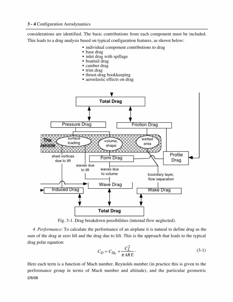
2. Fluid Mechanics: This viewpoint emphasizes the drag resulting from various fluidmechanics phenomena. This approach is important in conceiving a means to reduce drag. It alsoprovides a means of computing drag contributions in a systematic manner. Thinking in terms ofcontributionss from different physical effects, a typical drag breakdown would be:
• friction drag• form drag• induced drag• wave drag.
Each of these terms will be defined below. Figure 3-1 illustrates possible ways to find the totaldrag. It is based on a figure in Torenbeek’s book.11 He also has a good discussion of drag and itsestimation. Clearly, the subject can be confusing.
3. Aerodynamics: This approach combines the fluid mechanics viewpoint with more practicalconsiderations. From the aerodynamic design aspect it proves useful to think in terms ofcontributions from a variety of aircraft features. This includes effects due to the requirement totrim the aircraft, and interactions between the aerodynamics of the vehicle and both propulsioninduced flow effects and structural deformation effects. Within this context, several other
3 - 4 Configuration Aerodynamics
2/6/06
considerations are identified. The basic contributions from each component must be included.This leads to a drag analysis based on typical configuration features, as shown below:
• individual component contributions to drag• base drag• inlet drag with spillage• boattail drag• camber drag• trim drag• thrust-drag bookkeeping• aeroelastic effects on drag
Fig. 3-1. Drag breakdown possibilities (internal flow neglected).
4. Performance: To calculate the performance of an airplane it is natural to define drag as thesum of the drag at zero lift and the drag due to lift. This is the approach that leads to the typicaldrag polar equation:
CD = CD0 +CL2
π ARE. (3-1)
Here each term is a function of Mach number, Reynolds number (in practice this is given to theperformance group in terms of Mach number and altitude), and the particular geometric
report typos and errors to W.H. Mason Drag: An Introduction 3-5
2/6/06
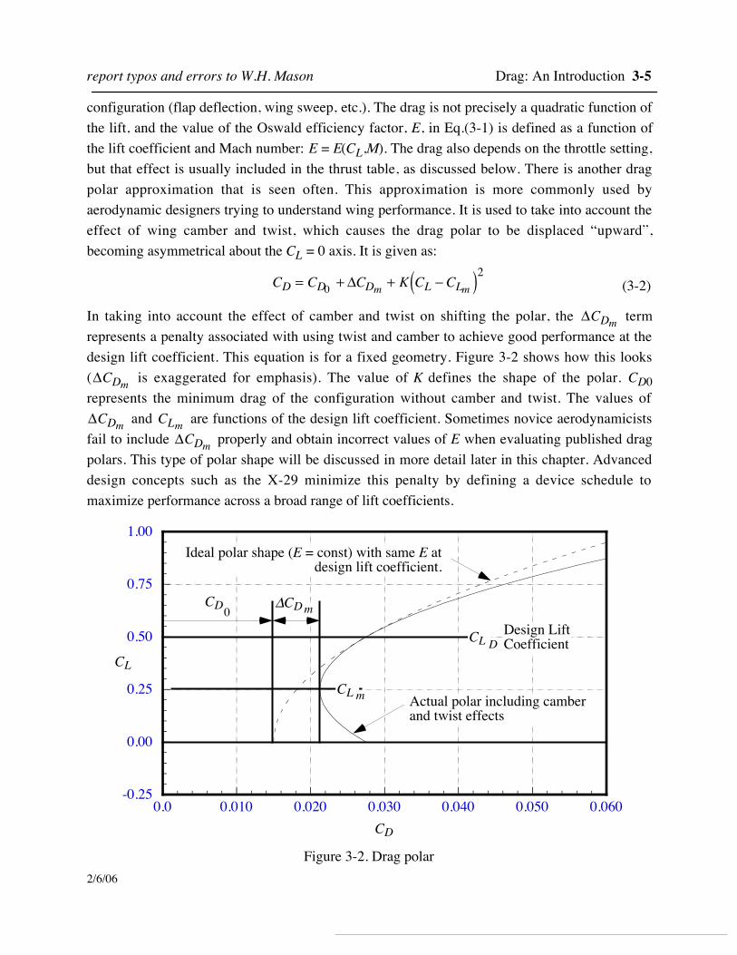
configuration (flap deflection, wing sweep, etc.). The drag is not precisely a quadratic function ofthe lift, and the value of the Oswald efficiency factor, E, in Eq.(3-1) is defined as a function ofthe lift coefficient and Mach number: E = E(CL,M). The drag also depends on the throttle setting,but that effect is usually included in the thrust table, as discussed below. There is another dragpolar approximation that is seen often. This approximation is more commonly used byaerodynamic designers trying to understand wing performance. It is used to take into account theeffect of wing camber and twist, which causes the drag polar to be displaced “upward”,becoming asymmetrical about the CL = 0 axis. It is given as:
CD = CD0 + ΔCDm + K CL − CLm( )2 (3-2)
In taking into account the effect of camber and twist on shifting the polar, the ΔCDm termrepresents a penalty associated with using twist and camber to achieve good performance at thedesign lift coefficient. This equation is for a fixed geometry. Figure 3-2 shows how this looks(ΔCDm is exaggerated for emphasis). The value of K defines the shape of the polar. CD0represents the minimum drag of the configuration without camber and twist. The values ofΔCDm and CLm are functions of the design lift coefficient. Sometimes novice aerodynamicistsfail to include ΔCDm properly and obtain incorrect values of E when evaluating published dragpolars. This type of polar shape will be discussed in more detail later in this chapter. Advanceddesign concepts such as the X-29 minimize this penalty by defining a device schedule tomaximize performance across a broad range of lift coefficients.
-0.25
0.00
0.25
0.50
0.75
1.00
0.0 0.010 0.020 0.030 0.040 0.050 0.060
CL
CD
CL m
CD0ΔCDm
Actual polar including camberand twist effects
Ideal polar shape (E = const) with same E atdesign lift coefficient.
CL DDesign LiftCoefficient
Figure 3-2. Drag polar
3 - 6 Configuration Aerodynamics
2/6/06
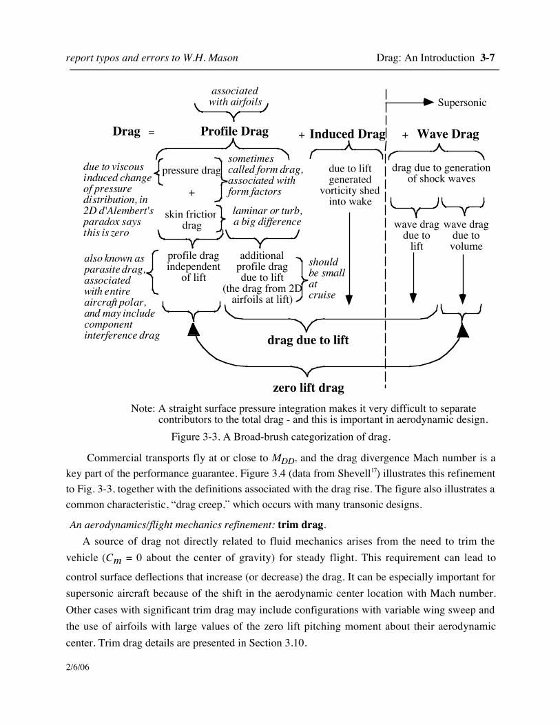
As mentioned above, basic drag nomenclature is frequently more confused than it needs to be,and sometimes the nomenclature gets in the way of technical discussions. The chart in Fig. 3-3provides a basic classification of drag for overview purposes. The aerodynamic configuration-specific approach to drag is not covered in fluid mechanics oriented aerodynamics texts, but isdescribed in aircraft design books. Two other good references are the books by Whitford12 andHuenecke.13 An approach to the evaluation of drag performance, including the efficiencyachieved on actual aircraft, was presented by Haines.14
We need to define several of these concepts in more detail. The most important overview ofaerodynamic drag for design has been given by Küchemann,15 and should be studied for acomplete understanding of drag concepts.
A fluid mechanics refinement: transonic wave drag.The broad-brush picture of drag presented in Fig. 3.3 suggests that wave drag appears
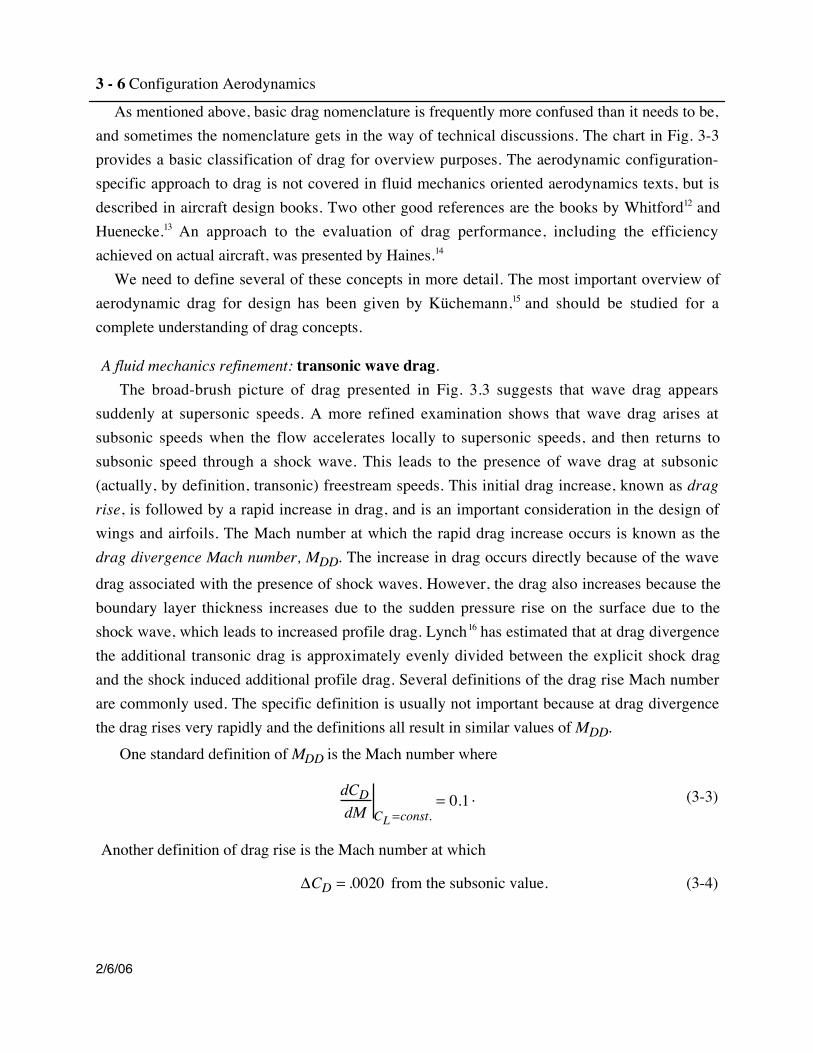
suddenly at supersonic speeds. A more refined examination shows that wave drag arises atsubsonic speeds when the flow accelerates locally to supersonic speeds, and then returns tosubsonic speed through a shock wave. This leads to the presence of wave drag at subsonic(actually, by definition, transonic) freestream speeds. This initial drag increase, known as dragrise, is followed by a rapid increase in drag, and is an important consideration in the design ofwings and airfoils. The Mach number at which the rapid drag increase occurs is known as thedrag divergence Mach number, MDD. The increase in drag occurs directly because of the wavedrag associated with the presence of shock waves. However, the drag also increases because theboundary layer thickness increases due to the sudden pressure rise on the surface due to theshock wave, which leads to increased profile drag. Lynch16 has estimated that at drag divergencethe additional transonic drag is approximately evenly divided between the explicit shock dragand the shock induced additional profile drag. Several definitions of the drag rise Mach numberare commonly used. The specific definition is usually not important because at drag divergencethe drag rises very rapidly and the definitions all result in similar values of MDD.
One standard definition of MDD is the Mach number where
dCDdM CL =const.
= 0.1 . (3-3)
Another definition of drag rise is the Mach number at which
ΔCD = .0020 from the subsonic value. (3-4)
report typos and errors to W.H. Mason Drag: An Introduction 3-7
2/6/06
Note: A straight surface pressure integration makes it very difficult to separate contributors to the total drag - and this is important in aerodynamic design.
Drag = Profile Drag + Induced Drag + Wave Drag
pressure drag
+
skin frictiondrag
associatedwith airfoils
profile dragindependent
of lift
due to liftgenerated
vorticity shedinto wake
drag due to generationof shock waves
wave dragdue to
lift
wave dragdue tovolume
additionalprofile dragdue to lift
(the drag from 2Dairfoils at lift)
laminar or turb,a big difference
shouldbe smallatcruise
sometimescalled form drag,associated withform factors
drag due to lift
due to viscousinduced changeof pressuredistribution, in2D d'Alembert'sparadox saysthis is zero
Supersonic
also known asparasite drag,associatedwith entireaircraft polar,and may includecomponentinterference drag
zero lift drag
Figure 3-3. A Broad-brush categorization of drag.
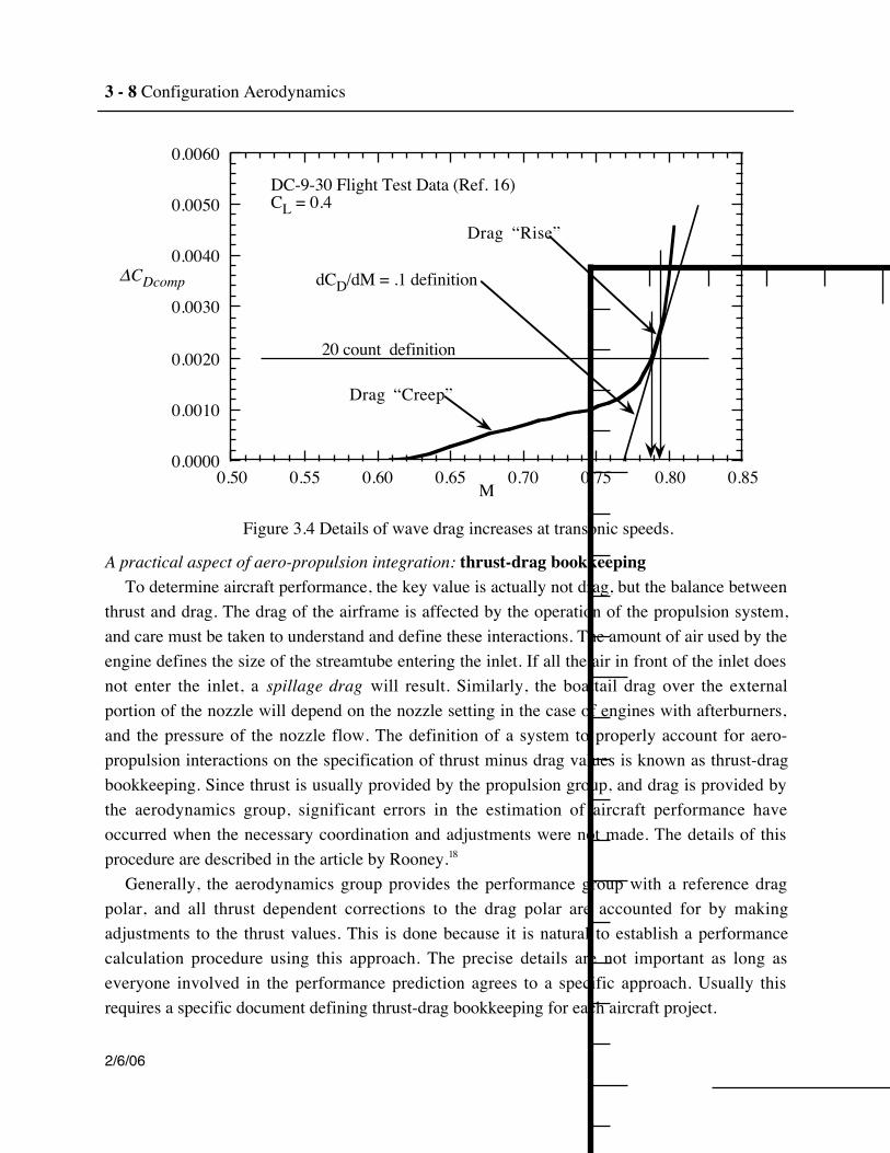
Commercial transports fly at or close to MDD, and the drag divergence Mach number is akey part of the performance guarantee. Figure 3.4 (data from Shevell17) illustrates this refinementto Fig. 3-3, together with the definitions associated with the drag rise. The figure also illustrates acommon characteristic, “drag creep,” which occurs with many transonic designs.
An aerodynamics/flight mechanics refinement: trim drag.A source of drag not directly related to fluid mechanics arises from the need to trim the
vehicle (Cm = 0 about the center of gravity) for steady flight. This requirement can lead to
control surface deflections that increase (or decrease) the drag. It can be especially important forsupersonic aircraft because of the shift in the aerodynamic center location with Mach number.Other cases with significant trim drag may include configurations with variable wing sweep andthe use of airfoils with large values of the zero lift pitching moment about their aerodynamiccenter. Trim drag details are presented in Section 3.10.
3 - 8 Configuration Aerodynamics
2/6/06
0.0000
0.0010
0.0020
0.0030
0.0040
0.0050
0.0060
0.50 0.55 0.60 0.65 0.70 0.75 0.80 0.85
ΔCDcomp
M
DC-9-30 Flight Test Data (Ref. 16)CL = 0.4
Drag “Creep”
20 count definition
dCD/dM = .1 definition
Drag “Rise”
Figure 3.4 Details of wave drag increases at transonic speeds.
A practical aspect of aero-propulsion integration: thrust-drag bookkeepingTo determine aircraft performance, the key value is actually not drag, but the balance between
thrust and drag. The drag of the airframe is affected by the operation of the propulsion system,and care must be taken to understand and define these interactions. The amount of air used by theengine defines the size of the streamtube entering the inlet. If all the air in front of the inlet doesnot enter the inlet, a spillage drag will result. Similarly, the boattail drag over the externalportion of the nozzle will depend on the nozzle setting in the case of engines with afterburners,and the pressure of the nozzle flow. The definition of a system to properly account for aero-propulsion interactions on the specification of thrust minus drag values is known as thrust-dragbookkeeping. Since thrust is usually provided by the propulsion group, and drag is provided bythe aerodynamics group, significant errors in the estimation of aircraft performance haveoccurred when the necessary coordination and adjustments were not made. The details of thisprocedure are described in the article by Rooney.18
Generally, the aerodynamics group provides the performance group with a reference dragpolar, and all thrust dependent corrections to the drag polar are accounted for by makingadjustments to the thrust values. This is done because it is natural to establish a performancecalculation procedure using this approach. The precise details are not important as long aseveryone involved in the performance prediction agrees to a specific approach. Usually thisrequires a specific document defining thrust-drag bookkeeping for each aircraft project.
report typos and errors to W.H. Mason Drag: An Introduction 3-9
2/6/06
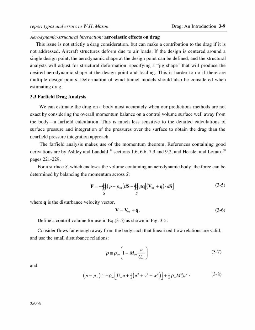
Aerodynamic-structural interaction: aeroelastic effects on dragThis issue is not strictly a drag consideration, but can make a contribution to the drag if it is
not addressed. Aircraft structures deform due to air loads. If the design is centered around asingle design point, the aerodynamic shape at the design point can be defined, and the structuralanalysts will adjust for structural deformation, specifying a “jig shape” that will produce thedesired aerodynamic shape at the design point and loading. This is harder to do if there aremultiple design points. Deformation of wind tunnel models should also be considered whenestimating drag.
3.3 Farfield Drag Analysis
We can estimate the drag on a body most accurately when our predictions methods are notexact by considering the overall momentum balance on a control volume surface well away fromthe body—a farfield calculation. This is much less sensitive to the detailed calculations ofsurface pressure and integration of the pressures over the surface to obtain the drag than thenearfield pressure integration approach.
The farfield analysis makes use of the momentum theorem. References containing goodderivations are by Ashley and Landahl,19 sections 1.6, 6.6, 7.3 and 9.2, and Heaslet and Lomax,20
pages 221-229.For a surface S, which encloses the volume containing an aerodynamic body, the force can be
determined by balancing the momentum across S:
F = − p − p∞( )S∫∫ dS − ρq V∞ + q( ) ⋅ dS[ ]
S∫∫ (3-5)
where q is the disturbance velocity vector,V = V∞ + q . (3-6)
Define a control volume for use in Eq.(3-5) as shown in Fig. 3-5.
Consider flows far enough away from the body such that linearized flow relations are valid;and use the small disturbance relations:
ρ ≅ ρ∞ 1 − M∞uU∞
⎛ ⎝ ⎜
⎞ ⎠ ⎟ (3-7)
and
p − p∞( ) ≅ −ρ∞ U∞u + 12 u
2 + v2 + w2( )⎡⎣ ⎤⎦ +12 ρ∞M∞
2u2 . (3-8)
3 - 10 Configuration Aerodynamics
2/6/06
zy
xII
III r
aircraft at originI
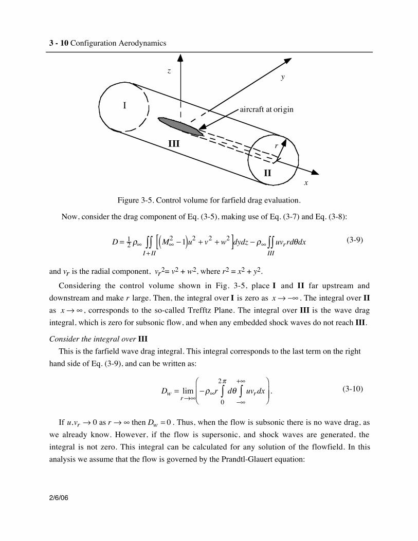
Figure 3-5. Control volume for farfield drag evaluation.
Now, consider the drag component of Eq. (3-5), making use of Eq. (3-7) and Eq. (3-8):
D = 12 ρ∞ M∞
2 −1( )u2 + v2 + w2[ ]dydz − ρ∞ uvrrdθdxIII∫∫
I + II∫∫ (3-9)
and vr is the radial component, vr2= v2 + w2, where r2 = x2 + y2.
Considering the control volume shown in Fig. 3-5, place I and II far upstream anddownstream and make r large. Then, the integral over I is zero as x→ −∞ . The integral over IIas x→ ∞ , corresponds to the so-called Trefftz Plane. The integral over III is the wave dragintegral, which is zero for subsonic flow, and when any embedded shock waves do not reach III.
Consider the integral over IIIThis is the farfield wave drag integral. This integral corresponds to the last term on the right
hand side of Eq. (3-9), and can be written as:
Dw = limr→∞
−ρ∞r dθ0
2π
∫ uvrdx−∞
+∞
∫⎛
⎝ ⎜ ⎜
⎞
⎠ ⎟ ⎟ .
(3-10)
If u,vr → 0 as r → ∞ then Dw = 0 . Thus, when the flow is subsonic there is no wave drag, aswe already know. However, if the flow is supersonic, and shock waves are generated, theintegral is not zero. This integral can be calculated for any solution of the flowfield. In thisanalysis we assume that the flow is governed by the Prandtl-Glauert equation:
report typos and errors to W.H. Mason Drag: An Introduction 3-11
2/6/06
1 −M∞2( )φxx + φyy + φzz = 0 , (3-11)
which implies small disturbance flow. This is valid if the vehicle is highly streamlined, as anysupersonic vehicle must be. However, since far from the disturbance this equation will modelflows from any vehicle, this is not a significant restriction.
To obtain an expression for φ that can be used to calculate the farfield integral, assume that the
body can be represented by a distribution of sources on the x-axis (the aircraft looks very“slender” from far away). To illustrate the analysis, assume that the body is axisymmetric. Recallthat there are different forms for the subsonic and supersonic source:
φ = −14π
1x2 + β2r2
subsonic source↓
φ →0 as r→ ∞
, φ = −12π
1x 2 − β2r2
supersonic source↓
φ →0 as r→ ∞ exceptas r→ x
β
. (3-12)
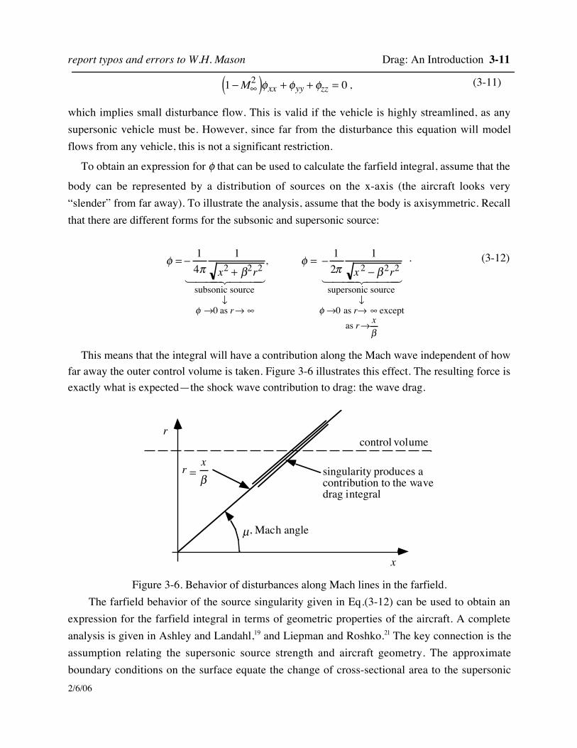
This means that the integral will have a contribution along the Mach wave independent of howfar away the outer control volume is taken. Figure 3-6 illustrates this effect. The resulting force isexactly what is expected—the shock wave contribution to drag: the wave drag.
x
rcontrol volume
µ, Mach angle
singularity produces acontribution to the wavedrag integral
r =xβ
Figure 3-6. Behavior of disturbances along Mach lines in the farfield.The farfield behavior of the source singularity given in Eq.(3-12) can be used to obtain an
expression for the farfield integral in terms of geometric properties of the aircraft. A completeanalysis is given in Ashley and Landahl,19 and Liepman and Roshko.21 The key connection is theassumption relating the supersonic source strength and aircraft geometry. The approximateboundary conditions on the surface equate the change of cross-sectional area to the supersonic
3 - 12 Configuration Aerodynamics
2/6/06
source strength: σ (x) = S '(x). One required assumption is that the cross-sectional area
distribution, S(x), satisfies S'(0) = S'(l) = 0. After some algebra the desired relation is obtained:
D θ( )w = −ρ∞U∞
2
4π′ ′ S (x1) ′ ′ S (x2)ln x1 − x2 dx1dx2
0
l
∫0
l
∫ . (3-13)
This is the wave drag integral. The standard method for evaluation of this integral is availablein a program known as the “Harris Wave Drag” program.22 That program determines the cross-sectional area distribution of the aircraft and then evaluates the integral numerically. Note that asgiven above, the Mach number doesn’t appear explicitly. A refined analysis19 for bodies thataren’t extremely slender extends this approach by taking slices, or Mach cuts, of the area throughthe body at the Mach angle. This is how the Mach number dependence enters the analysis.Finally, for non-axisymmetric bodies the area associated with the Mach cuts changes for eachangle around the circumferential integral for the cylindrical integration over Region III in Fig. 3-5. Thus the area distribution must be computed for each angle. The total wave drag is then foundfrom
Dw =12π
D w θ( )0
2π
∫ dθ . (3-14)
Examples of the results obtained using this computational method are given in Section 3.7, adiscussion of the area rule.
Consider the integral over II
This is the first integral in Eq. (3-9), the induced drag integral:
Di = 12 ρ∞ M∞
2 −1( )u2 + v2 + w2[ ]−∞
∞
∫−∞
∞
∫ dydz, (3-15)
Note that many supersonic aerodynamicists call this the vortex drag, Dv, since it is associatedwith the trailing vortex system. However, it is in fact the induced drag. The term vortex drag isconfusing in view of the current use of the term “vortex” to denote effects associated with other
vortex flow effects. Far downstream, u → 0, and we are left with the v and w components of
velocity induced by the trailing vortex system. The trailing vortex sheet can be thought of as legsof a horseshoe vortex. Thus the integral becomes:
Di = 12 ρ∞ v2 + w2( )
−∞
∞
∫−∞
∞
∫ dydz, (3-16)
which relates the drag to the kinetic energy of the trailing vortex system.
report typos and errors to W.H. Mason Drag: An Introduction 3-13
2/6/06
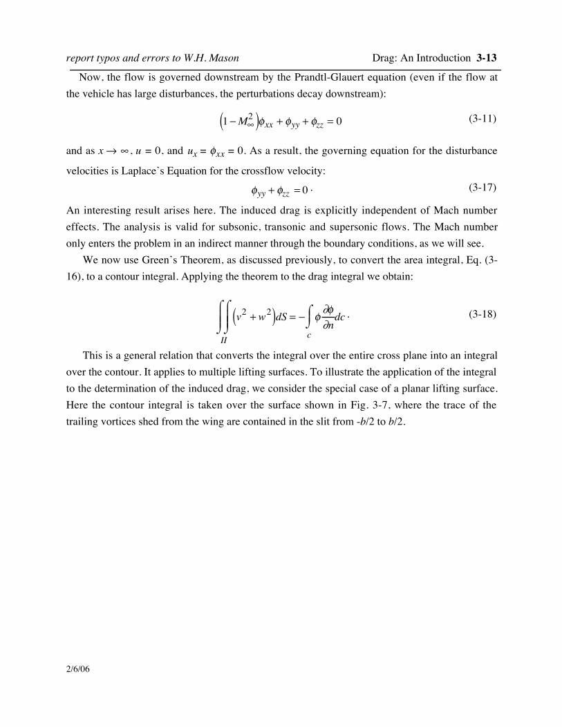
Now, the flow is governed downstream by the Prandtl-Glauert equation (even if the flow atthe vehicle has large disturbances, the perturbations decay downstream):
1 −M∞2( )φxx + φyy + φzz = 0 (3-11)
and as x → ∞ , u = 0, and ux = φxx = 0. As a result, the governing equation for the disturbance
velocities is Laplace’s Equation for the crossflow velocity:
φyy + φzz = 0 . (3-17)
An interesting result arises here. The induced drag is explicitly independent of Mach numbereffects. The analysis is valid for subsonic, transonic and supersonic flows. The Mach numberonly enters the problem in an indirect manner through the boundary conditions, as we will see.
We now use Green’s Theorem, as discussed previously, to convert the area integral, Eq. (3-16), to a contour integral. Applying the theorem to the drag integral we obtain:
v2 + w2( )dS = − φ∂φ∂n
c
⌠ ⌡ ⎮
II
⌠
⌡ ⎮ ⎮ ⌠
⌡ ⎮ ⎮ dc . (3-18)
This is a general relation that converts the integral over the entire cross plane into an integralover the contour. It applies to multiple lifting surfaces. To illustrate the application of the integralto the determination of the induced drag, we consider the special case of a planar lifting surface.Here the contour integral is taken over the surface shown in Fig. 3-7, where the trace of thetrailing vortices shed from the wing are contained in the slit from -b/2 to b/2.
3 - 14 Configuration Aerodynamics
2/6/06
z
y
RAD
BC
b/2-b/2
projection of trailing vortexsystem in y-z plane
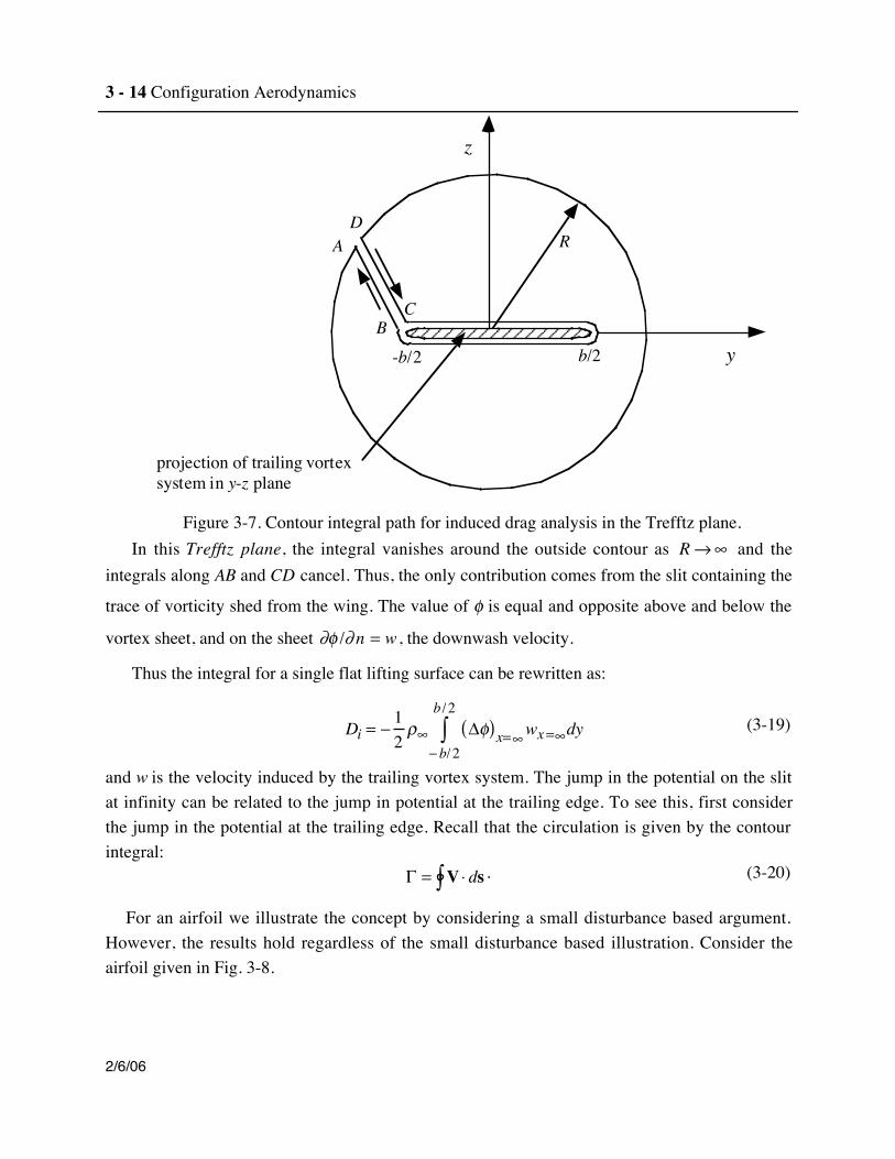
Figure 3-7. Contour integral path for induced drag analysis in the Trefftz plane.In this Trefftz plane, the integral vanishes around the outside contour as R→∞ and the
integrals along AB and CD cancel. Thus, the only contribution comes from the slit containing the
trace of vorticity shed from the wing. The value of φ is equal and opposite above and below the
vortex sheet, and on the sheet ∂φ /∂n = w , the downwash velocity.
Thus the integral for a single flat lifting surface can be rewritten as:
Di = −12ρ∞ Δφ( )x=∞wx=∞dy
− b/ 2
b / 2
∫ (3-19)
and w is the velocity induced by the trailing vortex system. The jump in the potential on the slitat infinity can be related to the jump in potential at the trailing edge. To see this, first considerthe jump in the potential at the trailing edge. Recall that the circulation is given by the contourintegral:
Γ = V ⋅ ds∫ . (3-20)
For an airfoil we illustrate the concept by considering a small disturbance based argument.However, the results hold regardless of the small disturbance based illustration. Consider theairfoil given in Fig. 3-8.
report typos and errors to W.H. Mason Drag: An Introduction 3-15
2/6/06
φx
φx
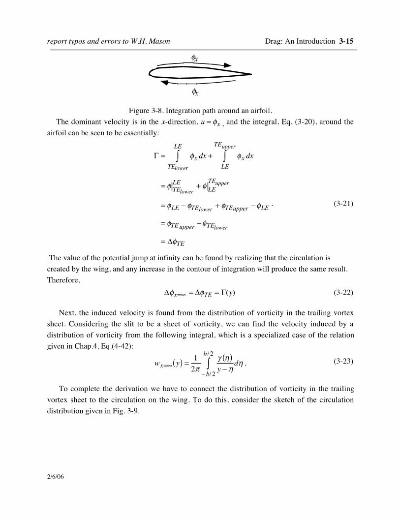
Figure 3-8. Integration path around an airfoil.The dominant velocity is in the x-direction, u = φx , and the integral, Eq. (3-20), around the
airfoil can be seen to be essentially:
Γ = φx dxTElower
LE
∫ + φx dxLE
TEupper
∫
= φ TElowerLE + φ LE
TEupper
= φLE − φTElower + φTEupper −φLE
= φTEupper −φTElower
= ΔφTE
. (3-21)
The value of the potential jump at infinity can be found by realizing that the circulation iscreated by the wing, and any increase in the contour of integration will produce the same result.Therefore,
Δφx=∞ = ΔφTE = Γ(y) (3-22)
Next, the induced velocity is found from the distribution of vorticity in the trailing vortexsheet. Considering the slit to be a sheet of vorticity, we can find the velocity induced by adistribution of vorticity from the following integral, which is a specialized case of the relationgiven in Chap.4, Eq.(4-42):
wx=∞ y( ) = 12π
γ η( )y − η
dη− b/ 2
b / 2
∫ . (3-23)
To complete the derivation we have to connect the distribution of vorticity in the trailingvortex sheet to the circulation on the wing. To do this, consider the sketch of the circulationdistribution given in Fig. 3-9.
3 - 16 Configuration Aerodynamics
2/6/06
Γ
γdη
y
dηdΓdη
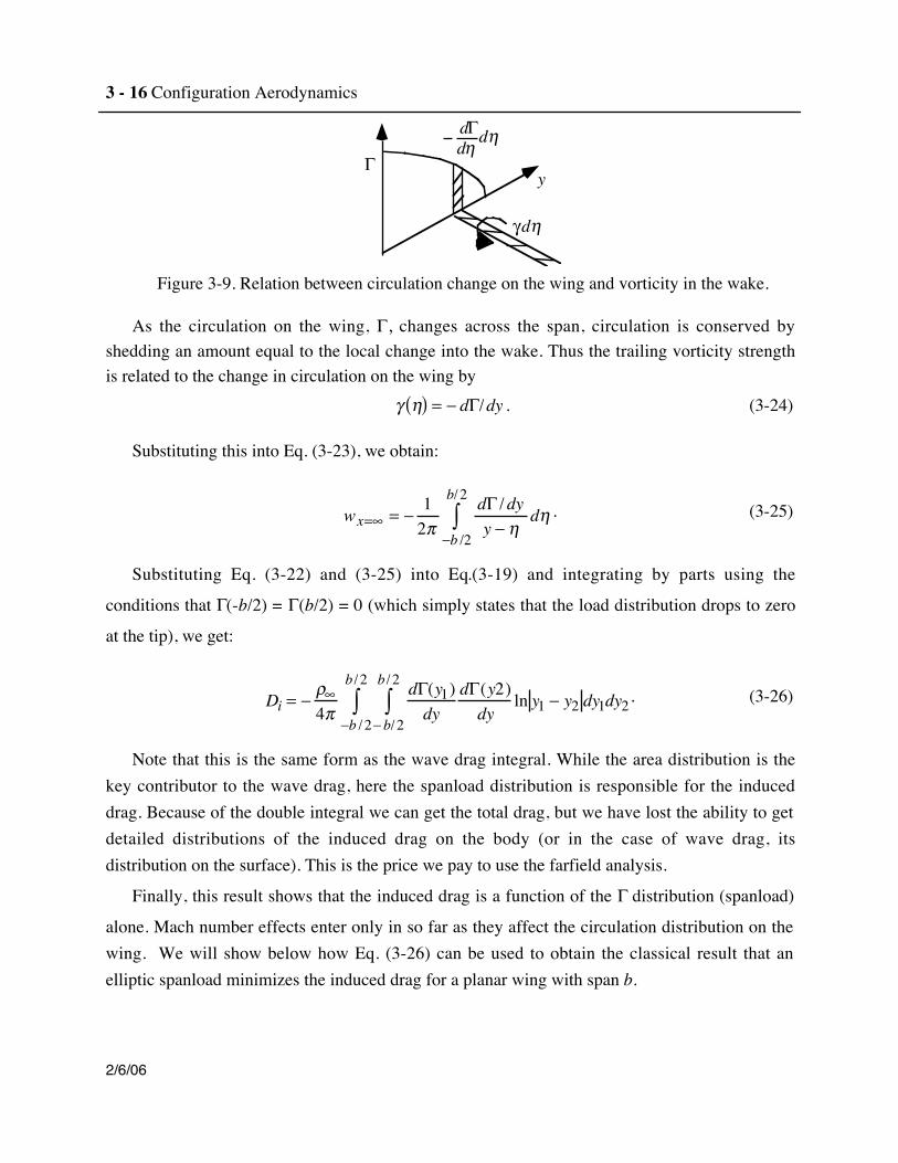
Figure 3-9. Relation between circulation change on the wing and vorticity in the wake.
As the circulation on the wing, Γ , changes across the span, circulation is conserved byshedding an amount equal to the local change into the wake. Thus the trailing vorticity strengthis related to the change in circulation on the wing by
γ η( ) = − dΓ/dy . (3-24)
Substituting this into Eq. (3-23), we obtain:
wx=∞ = −12π
dΓ /dyy − η
dη−b /2
b/ 2
∫ . (3-25)
Substituting Eq. (3-22) and (3-25) into Eq.(3-19) and integrating by parts using the
conditions that Γ(-b/2) = Γ(b/2) = 0 (which simply states that the load distribution drops to zero
at the tip), we get:
Di = −ρ∞4π
dΓ(y1)dy
dΓ(y2)dy
ln y1 − y2 dy1− b/ 2
b / 2
∫−b / 2
b / 2
∫ dy2 . (3-26)
Note that this is the same form as the wave drag integral. While the area distribution is thekey contributor to the wave drag, here the spanload distribution is responsible for the induceddrag. Because of the double integral we can get the total drag, but we have lost the ability to getdetailed distributions of the induced drag on the body (or in the case of wave drag, itsdistribution on the surface). This is the price we pay to use the farfield analysis.
Finally, this result shows that the induced drag is a function of the Γ distribution (spanload)
alone. Mach number effects enter only in so far as they affect the circulation distribution on thewing. We will show below how Eq. (3-26) can be used to obtain the classical result that anelliptic spanload minimizes the induced drag for a planar wing with span b.
report typos and errors to W.H. Mason Drag: An Introduction 3-17
2/6/06
3.4 Induced Drag
The three-dimensional flowfield over a lifting surface (for which a horseshoe vortex systemis a very good conceptual model) produces a drag, even if the flow is inviscid. This is due to theeffective change in the angle of attack along the wing induced by the trailing vortex system. Thisinduced change of angle results in a local inclination of the force vector relative to thefreestream, and produces an “induced” drag. It is one part of the total drag due to lift, and istypically written as:
CDi =CL2
πARe. (3-27)
The small “e” in this equation is known as the span e. As we will saw above, the induceddrag is only a function of the spanload. Additional losses due to the fuselage and viscous effectsare included when a capital E, known as Oswald’s E, is used in this expression. Note thatalthough this notation is the most prevalent in use in the US aircraft industry, other notations arefrequently employed, and care must be taken when reading the literature to make sure that youunderstand the notation used.
When designing and evaluating wings, the question becomes: what is “e”, and how large canwe make it? The “conventional wisdom” is that for a planar surface, emax = 1, and for a non-planar surface or a combination of lifting surfaces, emax > 1, where the aspect ratio, AR, is basedon the projected span of the wing with the largest span.* However, studies searching for highere’s abound. The quest of the aerodynamicist is to find a fundamental way to increaseaerodynamic efficiency. In the ’70s, increased aerodynamic efficiency, e, was sought byexploiting non-planar surface concepts such as winglets and canard configurations. Indeed, theseconcepts are now commonly employed on new configurations. In the’80s, a great deal ofattention was devoted to the use of advanced wing tip shapes on nominally planar configurations.It is not clear however that the advanced wingtips result in theoretical e’s above unity. However,in practice these improved tip shapes help clean up the flowfield at the wing tip, reducingviscous effects and resulting in a reduction in drag. An excellent survey of induced drag andreduction prospects was written by Kroo for the Annual Review of Fluid Mechanics.23
To establish a technical basis for understanding the drag due to lift of wings, singly and incombination, three concepts must be discussed: farfield drag (the Trefftz plane), Munk’s StaggerTheorem for design of multiple lifting surfaces, and, to understand additional drag above theinduced drag due to “e,” it is appropriate in introduce the concept of leading edge suction. Herewe will discuss the induced drag. Subsequent sections address Munk’s Stagger Theorem (Section3.6) and leading edge suction (Section 3.9)
* However, e is not too much bigger than unity for practical configurations.
3 - 18 Configuration Aerodynamics
2/6/06
In the last section we derived the expression for the drag due to the trailing vortex system.The far downstream location of this face of the control volume is known as the Trefftz plane.Here we explain the physical basis of the idea of the Trefftz plane following Ashley andLandahl19 almost verbatim. An alternate and valuable procedure has been described by Sears.24
The Trefftz PlaneThe idea:1. Far downstream the motion produced by the trailing vortices becomes 2D in
the y-z plane (no induced velocity in the x-direction).2. For a wing moving at a speed U∞ through the fluid at rest, an amount of
mechanical work DiU∞ is done on the fluid per unit time. Since the fluid isnondissipative (potential flow), it can store energy in kinetic form only.Therefore, the work DiU∞ must show up as the value of kinetic energycontained in a length U∞ of the distant wake.
and:3. The vortices in the trailing vortex system far downstream can be used to find
the induced drag.The Trefftz Plane is a y-z plane far downstream, so that all motion is in the crossflow plane (y-
z), and no velocity is induced in the x-direction, u = U∞. For a single planar lifting surface, the
expression for drag was found to be:
Di = −ρ∞4π
dΓ(y1)dy
dΓ(y2)dy
ln y1 − y2 dy1− b/ 2
b / 2
∫−b / 2
b / 2
∫ dy2 . (3-26)
The usual means of evaluating the induced drag integral is to represent Γ as a Fourier Series,
Γ =U∞b An sin nθn=1
∞∑ . (3-28)
The unknown values of the An’s are found from a Fourier series analysis, where Γ(y) is knownfrom an analysis of the configuration. Panel or vortex lattice methods can be used to find Γ(y).Vortex lattice methods are described briefly in Chapter 6. Integration of the drag integral withthis form of Γ results in:
Di =πρ∞U∞
2b2
8nAn2
n=1
∞∑ (3-29)
and
L =π4ρ∞U∞
2b2A1 , (3-30)
report typos and errors to W.H. Mason Drag: An Introduction 3-19
2/6/06
which are the classical results frequently derived using lifting line theory. Note that the liftdepends on the first term of the series, whereas all of the components contribute to the drag.Putting the expressions for lift and drag into coefficient form, and then replacing the A1 term inthe drag integral by its definition in terms of the lift coefficient leads to the classical result:
CDi =CL2
πARe(3-31)
where:
e =1
1 + n AnA1
⎛ ⎝ ⎜
⎞ ⎠ ⎟ 2
n= 2
∞∑
⎡
⎣ ⎢ ⎢
⎤
⎦ ⎥ ⎥
. (3-32)
These expressions show that emax = 1 for a planar lifting surface. However, if the slitrepresenting the trailing vortex system is not a simple flat surface, and CDi is based on theprojected span, a nonplanar or multiple lifting surface system can result in values of e > 1. Inparticular, biplane theory addresses the multiple lifting surface case, see Thwaites25 for a detaileddiscussion. If the wing is twisted, and the shape of the spanload changes as the lift changes, thene is not a constant, independent of the lift coefficient.
It is important to understand that the induced drag contribution to the drag due to lift assumesthat the airfoil sections in the wing are operating perfectly, as if in a two-dimensional potentialflow that has been reoriented relative to the freestream velocity at the angle associated with theeffects of the trailing vortex system. Wings can be designed to operate very close to theseconditions.
We conclude from this discussion:
1. Regardless of the wing planform(s), induced drag is a function of circulationdistribution alone, independent of Mach number except in the manner which Machnumber influences the circulation distribution (a minor effect in subsonic/transonicflow).
2. Given Γ, “e” can be determined by finding the An’s of the Fourier series for thesimple planar wing case. Other methods are required for nonplanar systems.3. Extra drag due to the airfoil’s inability to create lift ideally must be added over andabove the induced drag (our analysis here assumes that the airfoils operate perfectlyin a two-dimensional sense; there is no drag due to lift in two-dimensional flow).
3.5 Program LIDRAGFor single planar surfaces, a simple Fourier analysis of the spanload to determine the “e”
using a Fast Fourier Transform is available from the code LIDRAG. The user’s manual is given
3 - 20 Configuration Aerodynamics
2/6/06
in Appendix D.3. Numerous other methods could be used. For reference, note that the “e” for anelliptic spanload is 1.0, and the “e” for a triangular spanload is 0.728. LIDRAG was written byDave Ives, and is employed in numerous aerodynamics codes.26
3.6 Multiple Lifting Surfaces and Munk's Stagger Theorem
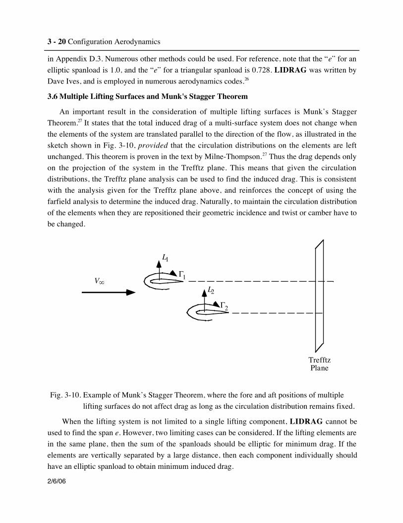
An important result in the consideration of multiple lifting surfaces is Munk’s StaggerTheorem.27 It states that the total induced drag of a multi-surface system does not change whenthe elements of the system are translated parallel to the direction of the flow, as illustrated in thesketch shown in Fig. 3-10, provided that the circulation distributions on the elements are leftunchanged. This theorem is proven in the text by Milne-Thompson.27 Thus the drag depends onlyon the projection of the system in the Trefftz plane. This means that given the circulationdistributions, the Trefftz plane analysis can be used to find the induced drag. This is consistentwith the analysis given for the Trefftz plane above, and reinforces the concept of using thefarfield analysis to determine the induced drag. Naturally, to maintain the circulation distributionof the elements when they are repositioned their geometric incidence and twist or camber have tobe changed.
V∞
L1
L2
Γ1
Γ2
TrefftzPlane
Fig. 3-10. Example of Munk’s Stagger Theorem, where the fore and aft positions of multiple lifting surfaces do not affect drag as long as the circulation distribution remains fixed.
When the lifting system is not limited to a single lifting component, LIDRAG cannot beused to find the span e. However, two limiting cases can be considered. If the lifting elements arein the same plane, then the sum of the spanloads should be elliptic for minimum drag. If theelements are vertically separated by a large distance, then each component individually shouldhave an elliptic spanload to obtain minimum induced drag.
report typos and errors to W.H. Mason Drag: An Introduction 3-21
2/6/06
When the system is composed of two lifting surfaces, or a lifting surface with dihedral breaks,including winglets, then a code by John Lamar28 is available to analyze the induced drag. Asoriginally developed, this code finds the minimum induced drag and the required spanloads for aprescribed lift and pitching moment constraint. It is known as LAMDES, and the user’s manualis given in Appendix D.4. This program is much more elaborate than LIDRAG. For subsonicflow the program will also estimate the camber and twist of the lifting surfaces required toachieve the minimum drag spanload. I extended this code to incorporate, approximately, theeffects of viscosity and find the system e for a user supplied spanload distribution.29
3.7 Zero Lift Drag: Friction and Form Drag EstimationEstimates of skin friction based on classical flat plate skin friction formulas can be used toprovide initial estimates of the friction and form drag portion of the zero lift drag. These arerequired for aerodynamic design studies using the rest of the methods described here. Thesesimple formulas are used in conceptual design in place of detailed boundary layer calculations,and provide good initial estimates until more detailed calculations using the boundary layermethods described in Chapter 10 are made. They are included here because they appear to havebeen omitted from current basic aerodynamics text books.* An excellent examination of themethods and accuracy of the approach described here was given by Paterson, MacWilkinson andBlackerby of Lockheed.30
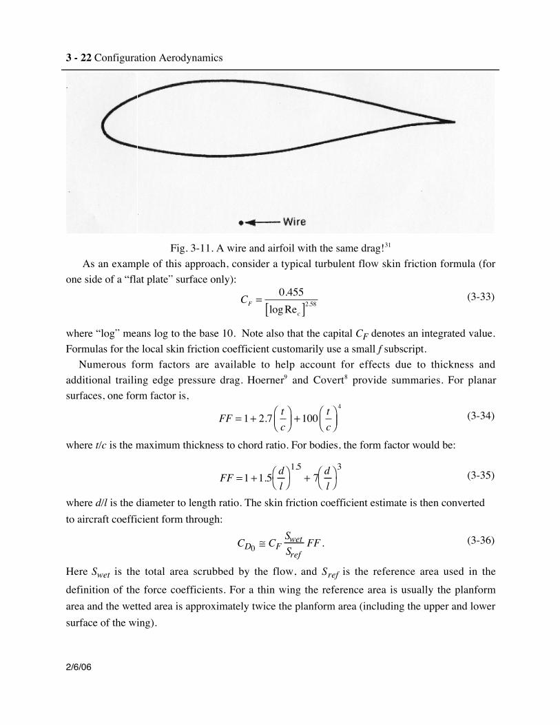
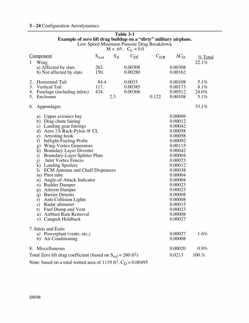
For a highly streamlined, aerodynamically clean shape the zero lift drag (friction and formdrag at subsonic speeds where there are no shock waves) should be mostly due to thesecontributions, and can be estimated using skin friction formulas. However, Table 3-1, for atypical military attack airplane, shows that on this airplane only about two-thirds of the zero liftdrag is associated with skin friction and form drag. This illustrates the serious performancepenalties associated with seemingly small details. R.T. Jones31 has presented a striking figure,included here as Fig. 3-11, comparing the drag on a modern airfoil to that of a single wire. It’shard to believe, and it demonstrates the importance of streamlining. An accurate drag estimaterequires that these details be included.
Until recently, aerodynamicists assumed the flow on actual airplanes was completelyturbulent. However, as a result of work at NASA over the last decade and a half, someconfigurations can now take advantage of at least some laminar flow, with its significantreduction in friction drag. Advanced airfoils can have as much as 30 to 40% laminar flow.
* Expanded details including compressibility effects and mixed laminar-turbulent skin friction estimates are given inApp. D.5, FRICTION.
3 - 22 Configuration Aerodynamics
2/6/06
Fig. 3-11. A wire and airfoil with the same drag!31
As an example of this approach, consider a typical turbulent flow skin friction formula (forone side of a “flat plate” surface only):
CF =0.455
logRec[ ]2.58(3-33)
where “log” means log to the base 10. Note also that the capital CF denotes an integrated value.Formulas for the local skin friction coefficient customarily use a small f subscript.
Numerous form factors are available to help account for effects due to thickness andadditional trailing edge pressure drag. Hoerner9 and Covert8 provide summaries. For planarsurfaces, one form factor is,
FF = 1+ 2.7 tc
⎛⎝⎜
⎞⎠⎟+100 t
c⎛⎝⎜
⎞⎠⎟4
(3-34)
where t/c is the maximum thickness to chord ratio. For bodies, the form factor would be:
FF =1 +1.5 dl
⎛ ⎝
⎞ ⎠ 1.5
+ 7 dl
⎛ ⎝
⎞ ⎠ 3
(3-35)
where d/l is the diameter to length ratio. The skin friction coefficient estimate is then convertedto aircraft coefficient form through:
CD0 ≅ CFSwetSref
FF . (3-36)
Here Swet is the total area scrubbed by the flow, and Sref is the reference area used in thedefinition of the force coefficients. For a thin wing the reference area is usually the planformarea and the wetted area is approximately twice the planform area (including the upper and lowersurface of the wing).
report typos and errors to W.H. Mason Drag: An Introduction 3-23
2/6/06
Program FRICTION automates this procedure using slightly improved formulas for the skinfriction that include compressibility effects. The program computes the skin friction and formdrag over each component, including laminar and turbulent flow. The user can input either theMach and Reynolds numbers or the Mach number and altitude. The use of this program isdescribed in manual online together with the program. This analysis assumes that the aircraft ishighly streamlined. For many aircraft this is not the case. As discussed above, Table 3-1 providesan example of the significantly increased drag that results when developing an aircraft foroperational use.
Comment: On a tour of the final assembly lines of the Boeing 747 and 777 onFebruary 29, 1996, I observed that the 777 was much, much smootheraerodynamically than the 747. Clearly, a lot of the advanced performance of the 777is due to old-fashioned attention to detail. The aerodynamicists have apparentlyfinally convinced the manufacturing engineers of the importance of aerodynamiccleanliness. Think about this the next time you compare a Cessna 182 to the modernhomebuilts, as exemplified by the Lancairs and Glassairs.
3 - 24 Configuration Aerodynamics
2/6/06
Table 3-1Example of zero lift drag buildup on a “dirty” military airplane.
Low Speed Minimum Parasite Drag Breakdown M < .65, CL = 0.0
Component Swet Sπ CDf CDπ ΔCD % Total1 Wing 22.1%
a) Affected by slats 262. 0.00308 0.00308b) Not affected by slats 150. 0.00280 0.00162
2. Horizontal Tail 84.4 0.0033 0.00108 5.1%3. Vertical Tail 117. 0.00385 0.00173 8.1%4. Fuselage (including inlets) 434. 0.00306 0.00512 24.0%5. Enclosure 2.3 0.122 0.00108 5.1%
6. Appendages 33.1%
a) Upper avionics bay 0.00069b) Drag-chute fairing 0.00012c) Landing gear fairings 0.00042d) Aero 7A Rack-Pylon @ CL 0.00058e) Arresting hook 0.00058f) Inflight-Fueling Probe 0.00092g) Wing-Vortex Generators 0.00115h) Boundary Layer Diverter 0.00042i) Boundary-Layer Splitter Plate 0.00004j) Inlet Vortex Fences 0.00023k) Landing Spoilers 0.00012l) ECM Antenna and Chaff Dispensers 0.00038m) Pitot tube 0.00004n) Angle-of-Attack Indicator 0.00004o) Rudder Damper 0.00023p) Aileron Damper 0.00023q) Barrier Detents 0.00008r) Anti-Collision Lights 0.00008s) Radar altimeter 0.00015t) Fuel Dump and Vent 0.00023u) Airblast Rain Removal 0.00008v) Catapult Holdback 0.00027
7. Inlets and Exitsa) Powerplant (vents, etc.) 0.00027 1.6%b) Air Conditioning 0.00008
8. Miscellaneous 0.00020 0.9%Total Zero lift drag coefficient (based on Sref = 260 ft2) 0.0213 100.%Note: based on a total wetted area of 1119 ft2, CD = 0.00495
report typos and errors to W.H. Mason Drag: An Introduction 3-25
2/6/06
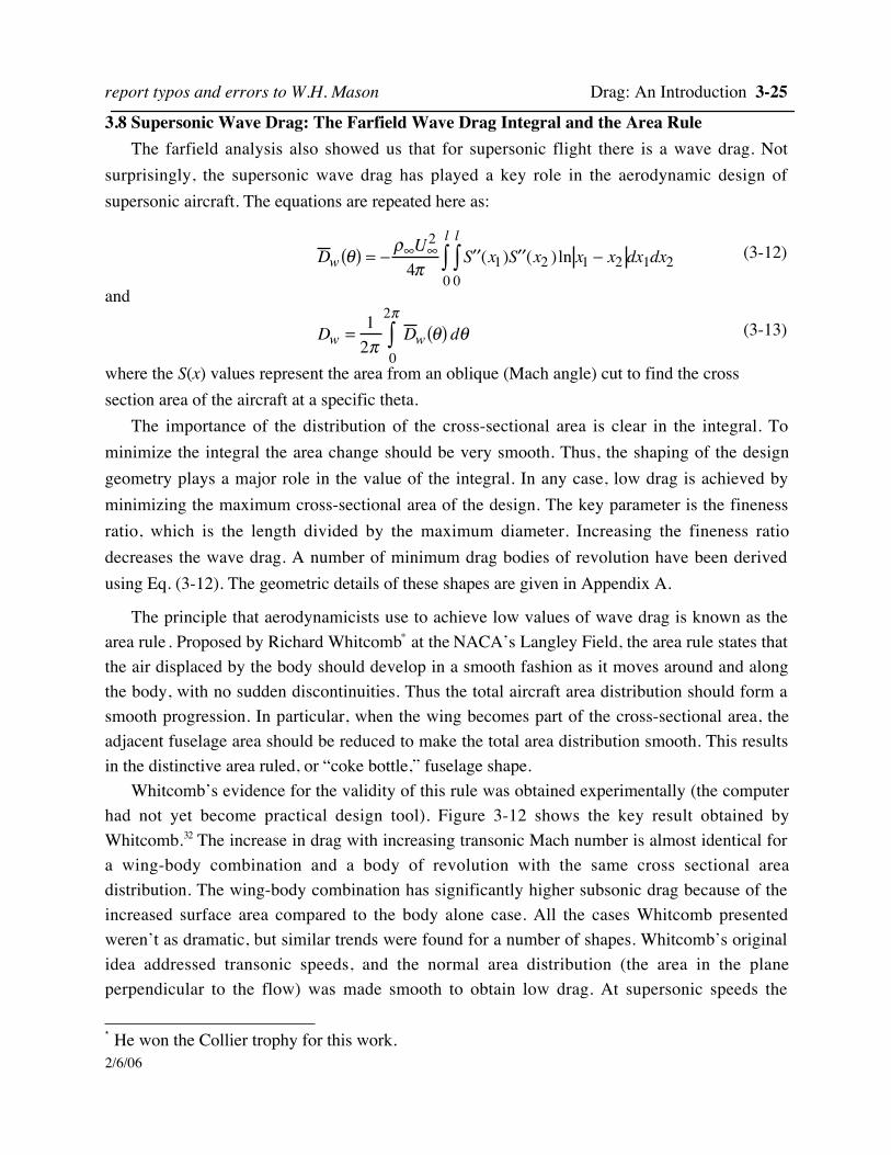
3.8 Supersonic Wave Drag: The Farfield Wave Drag Integral and the Area RuleThe farfield analysis also showed us that for supersonic flight there is a wave drag. Not
surprisingly, the supersonic wave drag has played a key role in the aerodynamic design ofsupersonic aircraft. The equations are repeated here as:
D w θ( ) = −ρ∞U∞
2
4π′ ′ S (x1) ′ ′ S (x2 )ln x1 − x2 dx1dx2
0
l
∫0
l
∫ (3-12)
and
Dw =12π
D w θ( )0
2π
∫ dθ (3-13)
where the S(x) values represent the area from an oblique (Mach angle) cut to find the crosssection area of the aircraft at a specific theta.
The importance of the distribution of the cross-sectional area is clear in the integral. Tominimize the integral the area change should be very smooth. Thus, the shaping of the designgeometry plays a major role in the value of the integral. In any case, low drag is achieved byminimizing the maximum cross-sectional area of the design. The key parameter is the finenessratio, which is the length divided by the maximum diameter. Increasing the fineness ratiodecreases the wave drag. A number of minimum drag bodies of revolution have been derivedusing Eq. (3-12). The geometric details of these shapes are given in Appendix A.
The principle that aerodynamicists use to achieve low values of wave drag is known as thearea rule . Proposed by Richard Whitcomb* at the NACA’s Langley Field, the area rule states thatthe air displaced by the body should develop in a smooth fashion as it moves around and alongthe body, with no sudden discontinuities. Thus the total aircraft area distribution should form asmooth progression. In particular, when the wing becomes part of the cross-sectional area, theadjacent fuselage area should be reduced to make the total area distribution smooth. This resultsin the distinctive area ruled, or “coke bottle,” fuselage shape.
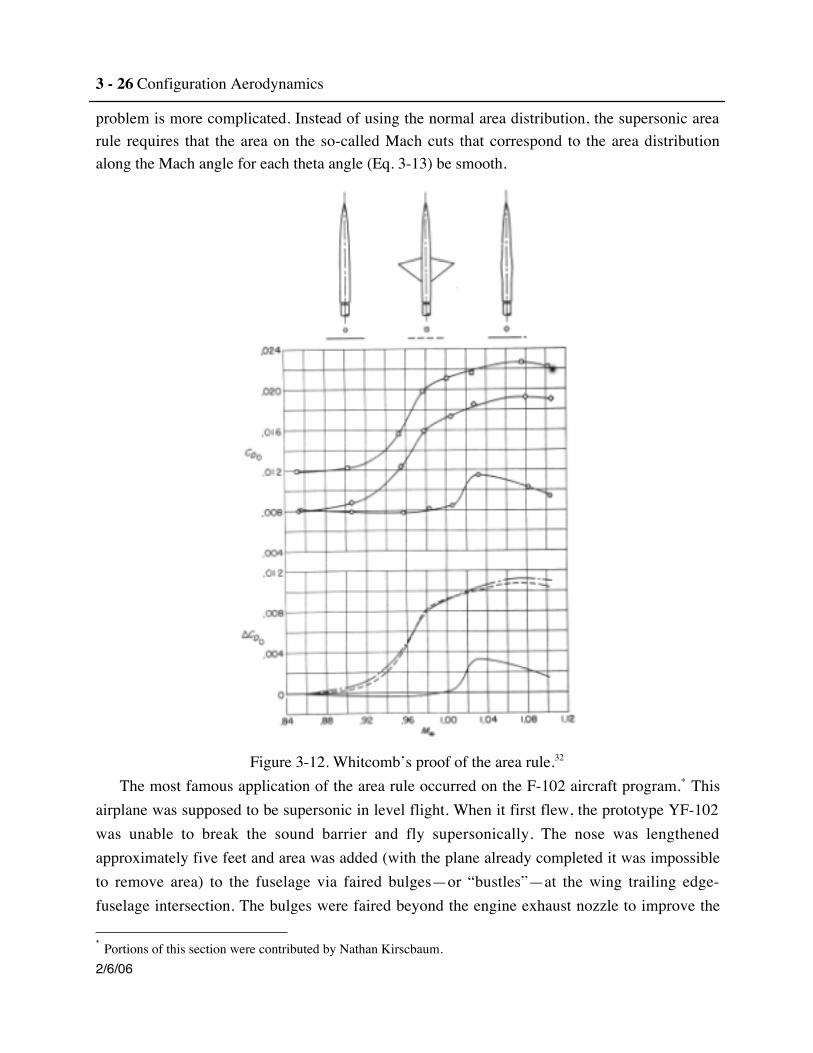
Whitcomb’s evidence for the validity of this rule was obtained experimentally (the computerhad not yet become practical design tool). Figure 3-12 shows the key result obtained byWhitcomb.32 The increase in drag with increasing transonic Mach number is almost identical fora wing-body combination and a body of revolution with the same cross sectional areadistribution. The wing-body combination has significantly higher subsonic drag because of theincreased surface area compared to the body alone case. All the cases Whitcomb presentedweren’t as dramatic, but similar trends were found for a number of shapes. Whitcomb’s originalidea addressed transonic speeds, and the normal area distribution (the area in the planeperpendicular to the flow) was made smooth to obtain low drag. At supersonic speeds the
* He won the Collier trophy for this work.
3 - 26 Configuration Aerodynamics
2/6/06
problem is more complicated. Instead of using the normal area distribution, the supersonic arearule requires that the area on the so-called Mach cuts that correspond to the area distributionalong the Mach angle for each theta angle (Eq. 3-13) be smooth.
Figure 3-12. Whitcomb’s proof of the area rule.32
The most famous application of the area rule occurred on the F-102 aircraft program.* Thisairplane was supposed to be supersonic in level flight. When it first flew, the prototype YF-102was unable to break the sound barrier and fly supersonically. The nose was lengthenedapproximately five feet and area was added (with the plane already completed it was impossibleto remove area) to the fuselage via faired bulges—or “bustles”—at the wing trailing edge-fuselage intersection. The bulges were faired beyond the engine exhaust nozzle to improve the * Portions of this section were contributed by Nathan Kirscbaum.
report typos and errors to W.H. Mason Drag: An Introduction 3-27
2/6/06
fineness ratio and area distribution. After these modifications, the prototype YF-102 was capableof penetrating deeper into the transonic region. However, it was still not capable of exceedingMach 1.0 in level flight. A complete redesign was necessary. It had to be done to continue thecontract.
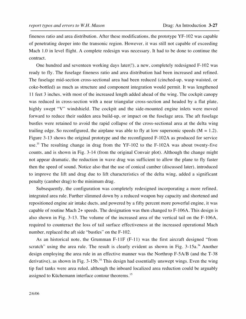
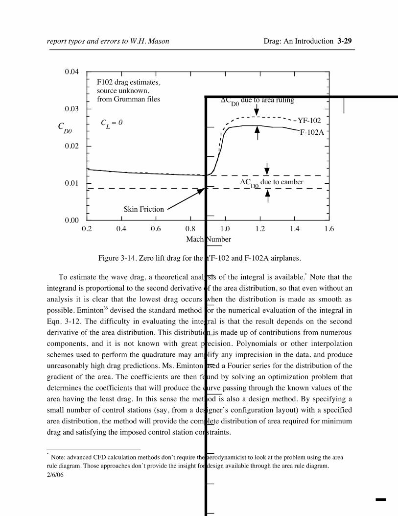
One hundred and seventeen working days later(!), a new, completely redesigned F-102 wasready to fly. The fuselage fineness ratio and area distribution had been increased and refined.The fuselage mid-section cross-sectional area had been reduced (cinched-up, wasp waisted, orcoke-bottled) as much as structure and component integration would permit. It was lengthened11 feet 3 inches, with most of the increased length added ahead of the wing. The cockpit canopywas reduced in cross-section with a near triangular cross-section and headed by a flat plate,highly swept “V” windshield. The cockpit and the side-mounted engine inlets were movedforward to reduce their sudden area build-up, or impact on the fuselage area. The aft fuselagebustles were retained to avoid the rapid collapse of the cross-sectional area at the delta wingtrailing edge. So reconfigured, the airplane was able to fly at low supersonic speeds (M = 1.2).Figure 3-13 shows the original prototype and the reconfigured F-102A as produced for serviceuse.33 The resulting change in drag from the YF-102 to the F-102A was about twenty-fivecounts, and is shown in Fig. 3-14 (from the original Convair plot). Although the change mightnot appear dramatic, the reduction in wave drag was sufficient to allow the plane to fly fasterthen the speed of sound. Notice also that the use of conical camber (discussed later), introducedto improve the lift and drag due to lift characteristics of the delta wing, added a significantpenalty (camber drag) to the minimum drag.
Subsequently, the configuration was completely redesigned incorporating a more refined,integrated area rule. Further slimmed down by a reduced weapon bay capacity and shortened andrepositioned engine air intake ducts, and powered by a fifty percent more powerful engine, it wascapable of routine Mach 2+ speeds. The designation was then changed to F-106A. This design isalso shown in Fig. 3-13. The volume of the increased area of the vertical tail on the F-106A,required to counteract the loss of tail surface effectiveness at the increased operational Machnumber, replaced the aft side “bustles” on the F-102.
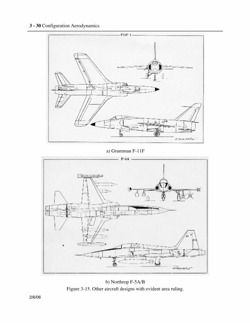
As an historical note, the Grumman F-11F (F-11) was the first aircraft designed “fromscratch” using the area rule. The result is clearly evident as shown in Fig. 3-15a.34 Anotherdesign employing the area rule in an effective manner was the Northrop F-5A/B (and the T-38derivative), as shown in Fig. 3-15b.34 This design had essentially unswept wings. Even the wingtip fuel tanks were area ruled, although the inboard localized area reduction could be arguablyassigned to Küchemann interface contour theorems.15
3 - 28 Configuration Aerodynamics
2/6/06
When considering the area rule, remember that this is only one part of successful airplanedesign.35 Moreover, extreme area ruling for a specific Mach number may significantly degradethe performance of the design at other Mach numbers.
Figure 3-13 Convair YF-102, F-102A, F-106A configuration evolution.33
report typos and errors to W.H. Mason Drag: An Introduction 3-29
2/6/06
0.00
0.01
0.02
0.03
0.04
0.2 0.4 0.6 0.8 1.0 1.2 1.4 1.6
F102 drag estimates, source unknown, from Grumman files
CD0
Mach Number
Skin Friction
ΔCD0 due to camber
F-102AYF-102
ΔCD0 due to area ruling
CL = 0
Figure 3-14. Zero lift drag for the YF-102 and F-102A airplanes.
To estimate the wave drag, a theoretical analysis of the integral is available.* Note that theintegrand is proportional to the second derivative of the area distribution, so that even without ananalysis it is clear that the lowest drag occurs when the distribution is made as smooth aspossible. Eminton36 devised the standard method for the numerical evaluation of the integral inEqn. 3-12. The difficulty in evaluating the integral is that the result depends on the secondderivative of the area distribution. This distribution is made up of contributions from numerouscomponents, and it is not known with great precision. Polynomials or other interpolationschemes used to perform the quadrature may amplify any imprecision in the data, and produceunreasonably high drag predictions. Ms. Eminton used a Fourier series for the distribution of thegradient of the area. The coefficients are then found by solving an optimization problem thatdetermines the coefficients that will produce the curve passing through the known values of thearea having the least drag. In this sense the method is also a design method. By specifying asmall number of control stations (say, from a designer’s configuration layout) with a specifiedarea distribution, the method will provide the complete distribution of area required for minimumdrag and satisfying the imposed control station constraints.
* Note: advanced CFD calculation methods don’t require the aerodynamicist to look at the problem using the arearule diagram. Those approaches don’t provide the insight for design available through the area rule diagram.
3 - 30 Configuration Aerodynamics
2/6/06
a) Grumman F-11F
b) Northrop F-5A/BFigure 3-15. Other aircraft designs with evident area ruling.
report typos and errors to W.H. Mason Drag: An Introduction 3-31
2/6/06
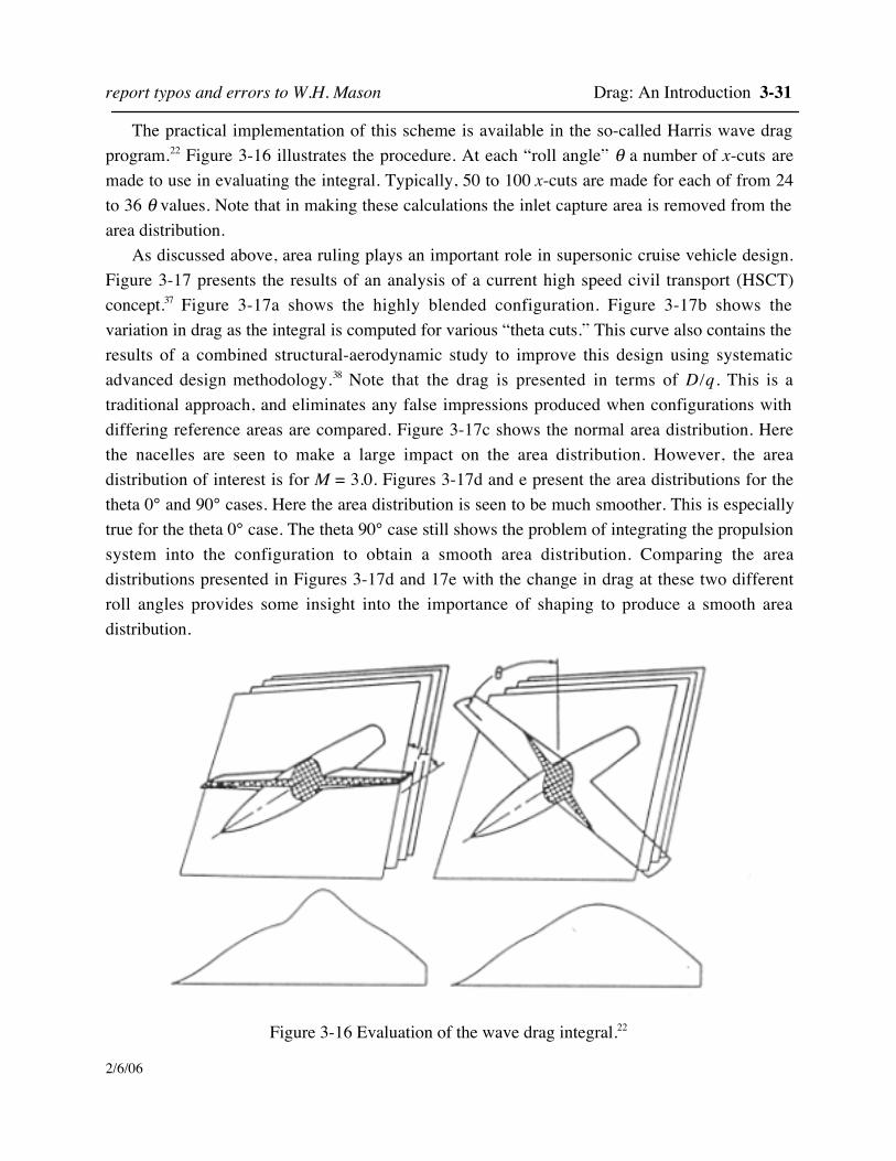
The practical implementation of this scheme is available in the so-called Harris wave dragprogram.22 Figure 3-16 illustrates the procedure. At each “roll angle” θ a number of x-cuts aremade to use in evaluating the integral. Typically, 50 to 100 x-cuts are made for each of from 24to 36 θ values. Note that in making these calculations the inlet capture area is removed from thearea distribution.
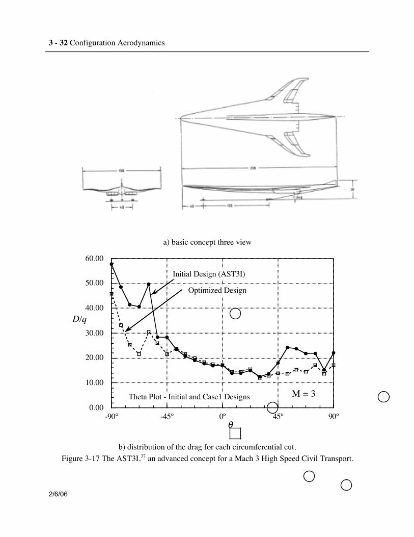
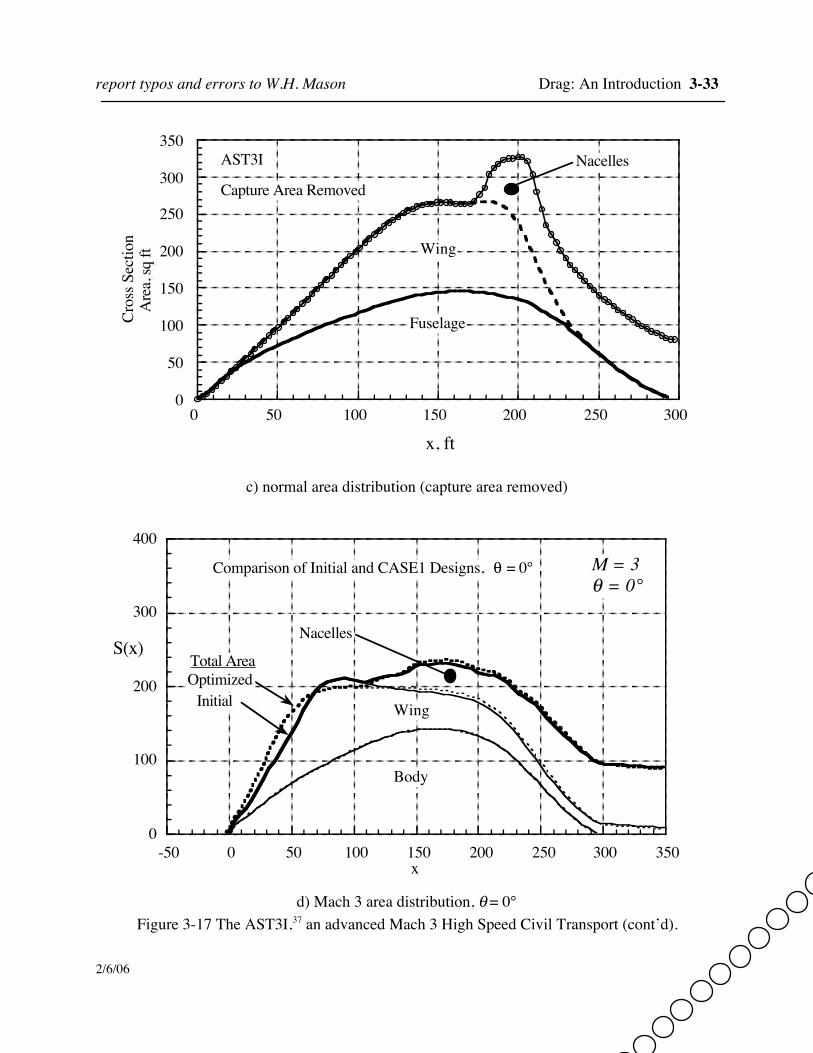
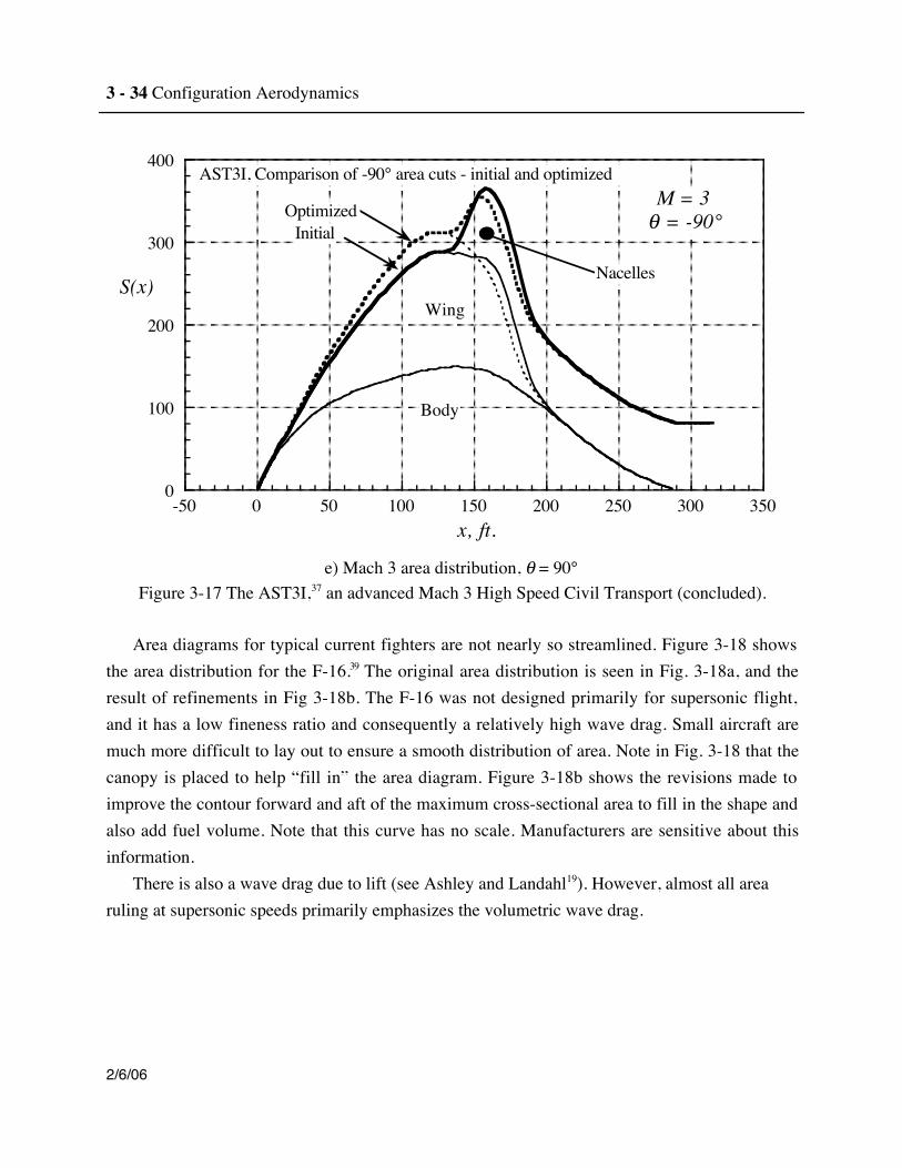
As discussed above, area ruling plays an important role in supersonic cruise vehicle design.Figure 3-17 presents the results of an analysis of a current high speed civil transport (HSCT)concept.37 Figure 3-17a shows the highly blended configuration. Figure 3-17b shows thevariation in drag as the integral is computed for various “theta cuts.” This curve also contains theresults of a combined structural-aerodynamic study to improve this design using systematicadvanced design methodology.38 Note that the drag is presented in terms of D/q. This is atraditional approach, and eliminates any false impressions produced when configurations withdiffering reference areas are compared. Figure 3-17c shows the normal area distribution. Herethe nacelles are seen to make a large impact on the area distribution. However, the areadistribution of interest is for M = 3.0. Figures 3-17d and e present the area distributions for thetheta 0° and 90° cases. Here the area distribution is seen to be much smoother. This is especiallytrue for the theta 0° case. The theta 90° case still shows the problem of integrating the propulsionsystem into the configuration to obtain a smooth area distribution. Comparing the areadistributions presented in Figures 3-17d and 17e with the change in drag at these two differentroll angles provides some insight into the importance of shaping to produce a smooth areadistribution.
Figure 3-16 Evaluation of the wave drag integral.22
3 - 32 Configuration Aerodynamics
2/6/06
a) basic concept three view
0.00
10.00
20.00
30.00
40.00
50.00
60.00
-90° -45° 0° 45° 90°
D/q
θ
Theta Plot - Initial and Case1 Designs M = 3
Initial Design (AST3I)
Optimized Design
b) distribution of the drag for each circumferential cut.Figure 3-17 The AST3I,37 an advanced concept for a Mach 3 High Speed Civil Transport.
report typos and errors to W.H. Mason Drag: An Introduction 3-33
2/6/06
0
50
100
150
200
250
300
350
0 50 100 150 200 250 300
Cros
s Sec
tion
Are
a, sq
ft
x, ft
Fuselage
Wing
NacellesAST3I
Capture Area Removed
c) normal area distribution (capture area removed)
0
100
200
300
400
-50 0 50 100 150 200 250 300 350
Comparison of Initial and CASE1 Designs, θ = 0°
S(x)
x
M = 3θ = 0°
OptimizedInitial
Body
Wing
Nacelles
Total Area
d) Mach 3 area distribution, θ = 0°Figure 3-17 The AST3I,37 an advanced Mach 3 High Speed Civil Transport (cont’d).
3 - 34 Configuration Aerodynamics
2/6/06
0
100
200
300
400
-50 0 50 100 150 200 250 300 350
AST3I, Comparison of -90° area cuts - initial and optimized
S(x)
x, ft.
M = 3θ = -90°Optimized
Initial
Body
Wing
Nacelles
e) Mach 3 area distribution, θ = 90°Figure 3-17 The AST3I,37 an advanced Mach 3 High Speed Civil Transport (concluded).
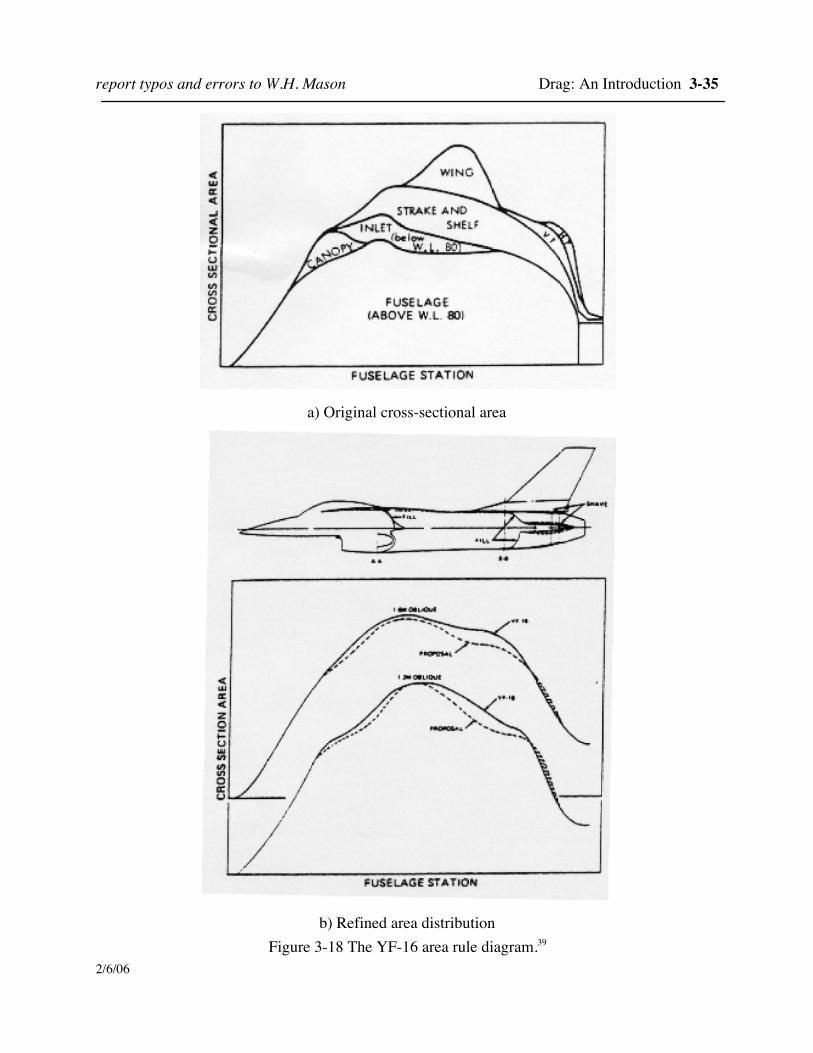
Area diagrams for typical current fighters are not nearly so streamlined. Figure 3-18 showsthe area distribution for the F-16.39 The original area distribution is seen in Fig. 3-18a, and theresult of refinements in Fig 3-18b. The F-16 was not designed primarily for supersonic flight,and it has a low fineness ratio and consequently a relatively high wave drag. Small aircraft aremuch more difficult to lay out to ensure a smooth distribution of area. Note in Fig. 3-18 that thecanopy is placed to help “fill in” the area diagram. Figure 3-18b shows the revisions made toimprove the contour forward and aft of the maximum cross-sectional area to fill in the shape andalso add fuel volume. Note that this curve has no scale. Manufacturers are sensitive about thisinformation.
There is also a wave drag due to lift (see Ashley and Landahl19). However, almost all arearuling at supersonic speeds primarily emphasizes the volumetric wave drag.
report typos and errors to W.H. Mason Drag: An Introduction 3-35
2/6/06
a) Original cross-sectional area
b) Refined area distributionFigure 3-18 The YF-16 area rule diagram.39
3 - 36 Configuration Aerodynamics
2/6/06
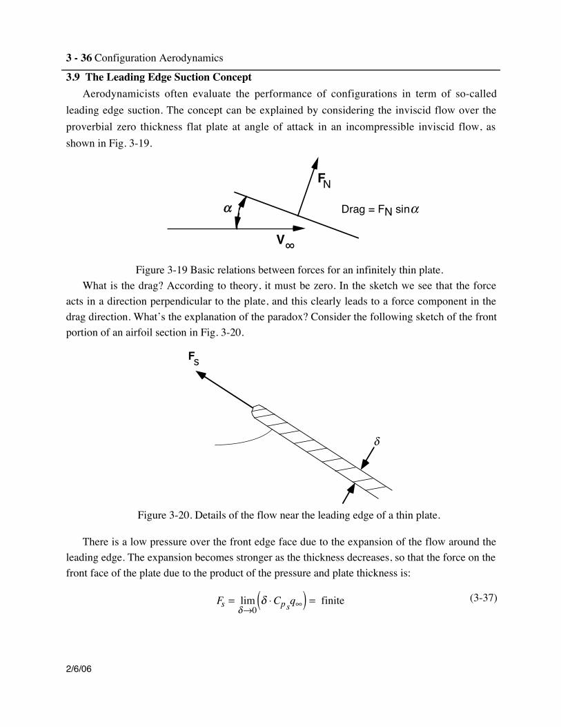
3.9 The Leading Edge Suction ConceptAerodynamicists often evaluate the performance of configurations in term of so-called
leading edge suction. The concept can be explained by considering the inviscid flow over theproverbial zero thickness flat plate at angle of attack in an incompressible inviscid flow, asshown in Fig. 3-19.
FN
V∞
α Drag = FN sinα
Figure 3-19 Basic relations between forces for an infinitely thin plate.What is the drag? According to theory, it must be zero. In the sketch we see that the force
acts in a direction perpendicular to the plate, and this clearly leads to a force component in thedrag direction. What’s the explanation of the paradox? Consider the following sketch of the frontportion of an airfoil section in Fig. 3-20.
δ
sF
Figure 3-20. Details of the flow near the leading edge of a thin plate.
There is a low pressure over the front edge face due to the expansion of the flow around theleading edge. The expansion becomes stronger as the thickness decreases, so that the force on thefront face of the plate due to the product of the pressure and plate thickness is:
Fs = limδ→0
δ ⋅Cpsq∞( ) = finite (3-37)
report typos and errors to W.H. Mason Drag: An Introduction 3-37
2/6/06
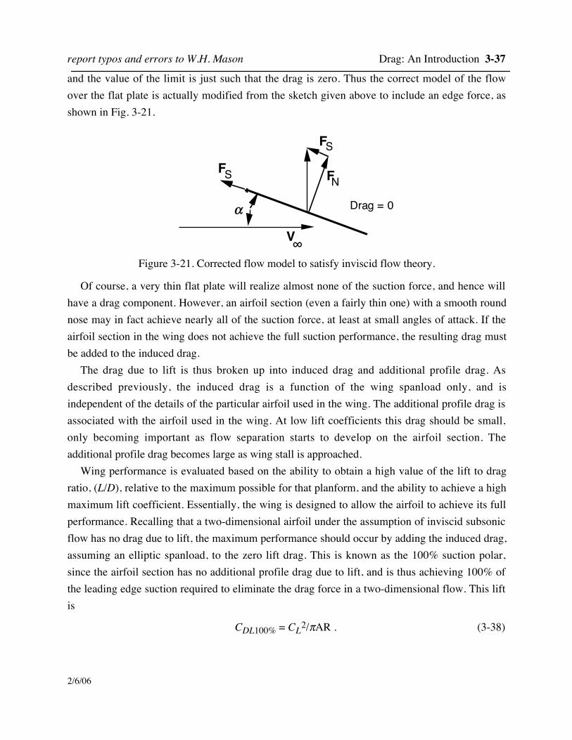
and the value of the limit is just such that the drag is zero. Thus the correct model of the flowover the flat plate is actually modified from the sketch given above to include an edge force, asshown in Fig. 3-21.
FN
V∞
α
F
FS
S
Drag = 0
Figure 3-21. Corrected flow model to satisfy inviscid flow theory.
Of course, a very thin flat plate will realize almost none of the suction force, and hence willhave a drag component. However, an airfoil section (even a fairly thin one) with a smooth roundnose may in fact achieve nearly all of the suction force, at least at small angles of attack. If theairfoil section in the wing does not achieve the full suction performance, the resulting drag mustbe added to the induced drag.
The drag due to lift is thus broken up into induced drag and additional profile drag. Asdescribed previously, the induced drag is a function of the wing spanload only, and isindependent of the details of the particular airfoil used in the wing. The additional profile drag isassociated with the airfoil used in the wing. At low lift coefficients this drag should be small,only becoming important as flow separation starts to develop on the airfoil section. Theadditional profile drag becomes large as wing stall is approached.
Wing performance is evaluated based on the ability to obtain a high value of the lift to dragratio, (L/D), relative to the maximum possible for that planform, and the ability to achieve a highmaximum lift coefficient. Essentially, the wing is designed to allow the airfoil to achieve its fullperformance. Recalling that a two-dimensional airfoil under the assumption of inviscid subsonicflow has no drag due to lift, the maximum performance should occur by adding the induced drag,assuming an elliptic spanload, to the zero lift drag. This is known as the 100% suction polar,since the airfoil section has no additional profile drag due to lift, and is thus achieving 100% ofthe leading edge suction required to eliminate the drag force in a two-dimensional flow. This liftis
CDL100% = CL2/πAR . (3-38)
3 - 38 Configuration Aerodynamics
2/6/06
At the other extreme, the worst case occurs when the airfoil fails to produce any efficient lift,such that the only force is normal to the surface and there is no edge or suction*[Footnote #6]force (0% leading edge suction). In this case the entire lifting force on the wing is the normalforce, and the polar can be determined by resolving that force into lift and drag components. Theequation for the 0% suction drag can be expressed in a variety of forms, starting with
CDL0%= CL tan(α−α0)} (3-39)
where α0 is the zero lift angle of attack. We also use the linear aerodynamic relation:
CL = CLα (α −α0 ) (3-40)
which can be solved for the angle of attack:
(α −α0) =CLCLα
. (3-41)
Finally, substitute Eqn. (3-41) into Eqn. (3-39) for the angle of attack as follows:
CDL0% = CL tan(α − α0) ≅ CL(α − α0)
≅ CLCLCLα
or
CDL0% ≅CL2
CLα. (3-42)
This equation for the 0% suction polar shows why this polar is often referred to as the“1/CLα” polar by aerodynamicists. Using this approach, effective wing performance is quoted in
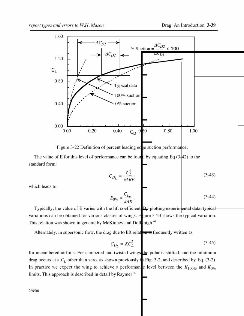
terms of the fraction of suction achieved, based on the difference between the actual drag and the100% and 0% suction values as shown in Figure 3-22. This figure illustrates how wings typicallyperform. The wing will approach the 100% level at low lift coefficients, and then as flowseparation starts to develop, the performance deteriorates. Eventually, the wing may have a dragsubstantially higher than the 0% suction value that was said above to be the worst case.
* On a swept wing the suction force is normal to the leading edge. The component of the leading edge suction forcein the streamwise direction is called the leading edge thrust.
report typos and errors to W.H. Mason Drag: An Introduction 3-39
2/6/06
0.00
0.40
0.80
1.20
1.60
0.00 0.20 0.40 0.60 0.80 1.00
100% suction
0% suction
Typical data
ΔCD1
ΔCD2% Suction =
ΔCD1
CL
ΔCD2
CD
x 100
Figure 3-22 Definition of percent leading edge suction performance.
The value of E for this level of performance can be found by equating Eq.(3-42) to thestandard form:
CDL =CL2
πARE(3-43)
which leads to:
E0% =CLαπAR
. (3-44)
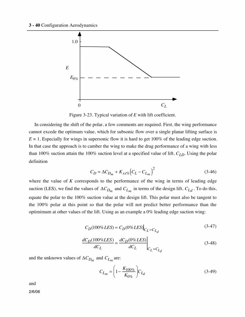
Typically, the value of E varies with the lift coefficient. By plotting experimental data, typicalvariations can be obtained for various classes of wings. Figure 3-23 shows the typical variation.This relation was shown in general by McKinney and Dollyhigh.40
Alternately, in supersonic flow, the drag due to lift relation is frequently written as
CDL = KCL2 (3-45)
for uncambered airfoils. For cambered and twisted wings the polar is shifted, and the minimumdrag occurs at a CL other than zero, as shown previously in Fig. 3-2, and described by Eq. (3-2).In practice we expect the wing to achieve a performance level between the K100% and K0%limits. This approach is described in detail by Raymer.41
3 - 40 Configuration Aerodynamics
2/6/06
1.0
E
0 CL
E0%
Figure 3-23. Typical variation of E with lift coefficient.
In considering the shift of the polar, a few comments are required. First, the wing performancecannot excede the optimum value, which for subsonic flow over a single planar lifting surface isE = 1. Especially for wings in supersonic flow it is hard to get 100% of the leading edge suction.In that case the approach is to camber the wing to make the drag performance of a wing with lessthan 100% suction attain the 100% suction level at a specified value of lift, CLD. Using the polardefinition
CD = ΔCDm + Kxx% CL − CLm( )2 (3-46)
where the value of K corresponds to the performance of the wing in terms of leading edgesuction (LES), we find the values of ΔCDm and CLm in terms of the design lift, CLd . To do this,
equate the polar to the 100% suction value at the design lift. This polar must also be tangent tothe 100% polar at this point so that the polar will not predict better performance than theoptimimum at other values of the lift. Using as an example a 0% leading edge suction wing:
CD(100%LES) = CD(0%LES)CL =CLd(3-47)
dCD(100%LES)dCL
=dCD(0%LES)
dCL CL =CLd
(3-48)
and the unknown values of ΔCDm and CLm are:
CLm = 1− K100%K0%
⎛ ⎝ ⎜
⎞ ⎠ ⎟ CLd (3-49)
and
report typos and errors to W.H. Mason Drag: An Introduction 3-41
2/6/06
ΔCDm = K100%CLd2 − K0% CLd − CLm( )2 . (3-50)
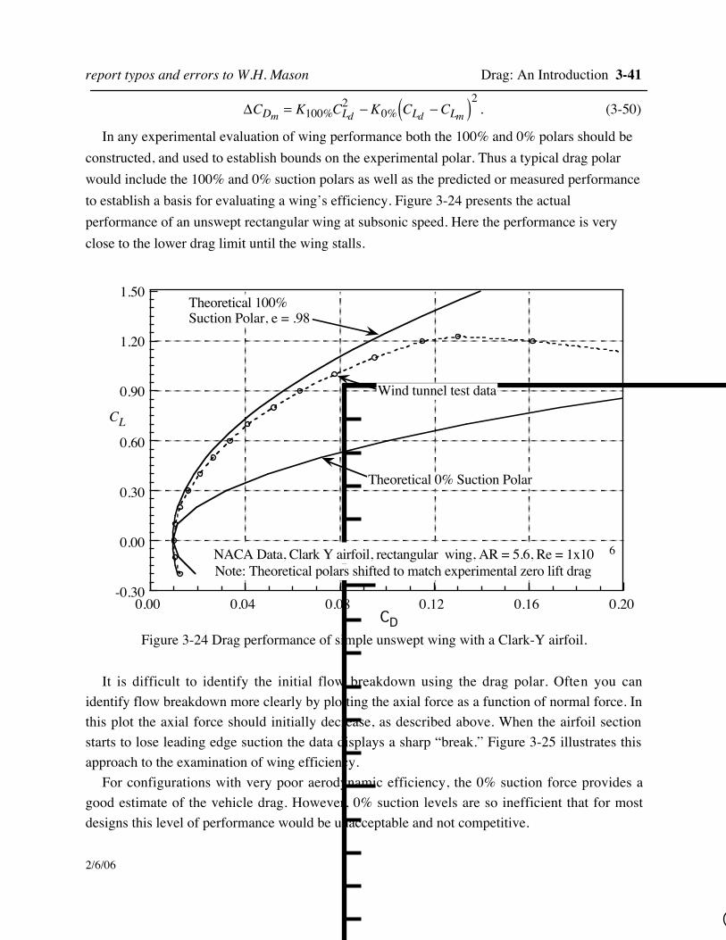
In any experimental evaluation of wing performance both the 100% and 0% polars should beconstructed, and used to establish bounds on the experimental polar. Thus a typical drag polarwould include the 100% and 0% suction polars as well as the predicted or measured performanceto establish a basis for evaluating a wing’s efficiency. Figure 3-24 presents the actualperformance of an unswept rectangular wing at subsonic speed. Here the performance is veryclose to the lower drag limit until the wing stalls.
-0.30
0.00
0.30
0.60
0.90
1.20
1.50
0.00 0.04 0.08 0.12 0.16 0.20
CL
CD
NACA Data, Clark Y airfoil, rectangular wing, AR = 5.6, Re = 1x10 6
Theoretical 100%Suction Polar, e = .98
Theoretical 0% Suction Polar
Wind tunnel test data
Note: Theoretical polars shifted to match experimental zero lift drag
Figure 3-24 Drag performance of simple unswept wing with a Clark-Y airfoil.
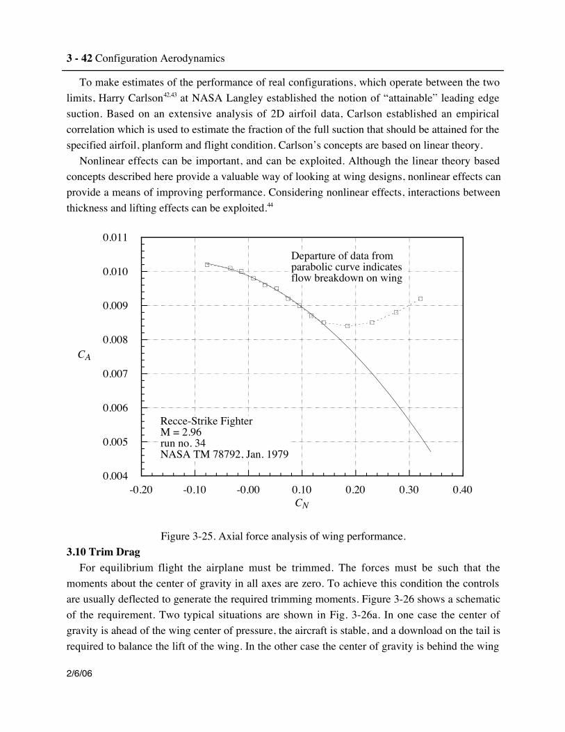
It is difficult to identify the initial flow breakdown using the drag polar. Often you canidentify flow breakdown more clearly by plotting the axial force as a function of normal force. Inthis plot the axial force should initially decrease, as described above. When the airfoil sectionstarts to lose leading edge suction the data displays a sharp “break.” Figure 3-25 illustrates thisapproach to the examination of wing efficiency.
For configurations with very poor aerodynamic efficiency, the 0% suction force provides agood estimate of the vehicle drag. However, 0% suction levels are so inefficient that for mostdesigns this level of performance would be unacceptable and not competitive.
3 - 42 Configuration Aerodynamics
2/6/06
To make estimates of the performance of real configurations, which operate between the twolimits, Harry Carlson42,43 at NASA Langley established the notion of “attainable” leading edgesuction. Based on an extensive analysis of 2D airfoil data, Carlson established an empiricalcorrelation which is used to estimate the fraction of the full suction that should be attained for thespecified airfoil, planform and flight condition. Carlson’s concepts are based on linear theory.
Nonlinear effects can be important, and can be exploited. Although the linear theory basedconcepts described here provide a valuable way of looking at wing designs, nonlinear effects canprovide a means of improving performance. Considering nonlinear effects, interactions betweenthickness and lifting effects can be exploited.44
0.004
0.005
0.006
0.007
0.008
0.009
0.010
0.011
-0.20 -0.10 -0.00 0.10 0.20 0.30 0.40
CA
CN
Recce-Strike FighterM = 2.96run no. 34NASA TM 78792, Jan. 1979
Departure of data fromparabolic curve indicatesflow breakdown on wing
Figure 3-25. Axial force analysis of wing performance.3.10 Trim Drag
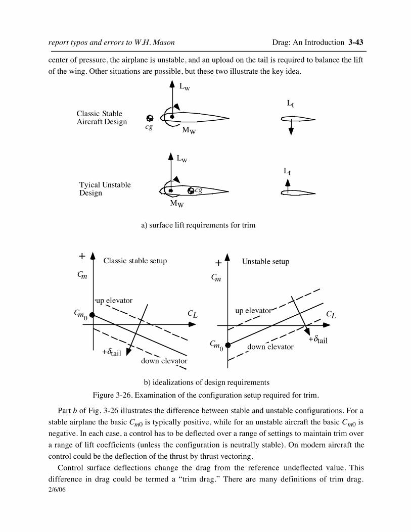
For equilibrium flight the airplane must be trimmed. The forces must be such that themoments about the center of gravity in all axes are zero. To achieve this condition the controlsare usually deflected to generate the required trimming moments. Figure 3-26 shows a schematicof the requirement. Two typical situations are shown in Fig. 3-26a. In one case the center ofgravity is ahead of the wing center of pressure, the aircraft is stable, and a download on the tail isrequired to balance the lift of the wing. In the other case the center of gravity is behind the wing
report typos and errors to W.H. Mason Drag: An Introduction 3-43
2/6/06
center of pressure, the airplane is unstable, and an upload on the tail is required to balance the liftof the wing. Other situations are possible, but these two illustrate the key idea.
Lw
Lt
MW
Lt
Lw
MW
Classic StableAircraft Design
Tyical UnstableDesign
+Cm
CLCm0
+Cm
CL
Cm0
Classic stable setup Unstable setup
+δtail
+δtail
a) surface lift requirements for trim
b) idealizations of design requirements
cg
cg
up elevator
down elevator
up elevator
down elevator
Figure 3-26. Examination of the configuration setup required for trim.
Part b of Fig. 3-26 illustrates the difference between stable and unstable configurations. For astable airplane the basic Cm0 is typically positive, while for an unstable aircraft the basic Cm0 isnegative. In each case, a control has to be deflected over a range of settings to maintain trim overa range of lift coefficients (unless the configuration is neutrally stable). On modern aircraft thecontrol could be the deflection of the thrust by thrust vectoring.
Control surface deflections change the drag from the reference undeflected value. Thisdifference in drag could be termed a “trim drag.” There are many definitions of trim drag.
3 - 44 Configuration Aerodynamics
2/6/06
Definitions differ because it is difficult to be precise in defining trim drag. Some definitionscontain only the drag due to the lift of the trimming surface. Some analyses allow for a negativetrim drag. However, for a given flight condition the total lift must be fixed, and any change in lifton the trimming surface requires a change in lift, and hence drag, on the primary surface. On awell-designed aircraft the trim drag should be small. Canard concepts are often consideredadvantageous because both the canard and wing supply positive lift to trim, whereas fortraditional aft-tail configurations the tail load is negative and the wing must operate at a higherlift to compensate. However, for modern aft-tail designs the tail load is near zero, resulting inlittle trim drag.
Trim drag has always been an important consideration in airplane design. However, trim dragbecame especially important with the development of stability and control augmentation systemsthat allowed the designer much greater freedom in the choice of a center of gravity location.Natural static stability was no longer required. The static stability condition had frequently madeit difficult to obtain minimum trim drag. This meant that trim drag could become a key criteriafor the placement of the center of gravity in a configuration (this is part of the motivation for so-called control configured vehicle, CCV, concepts).
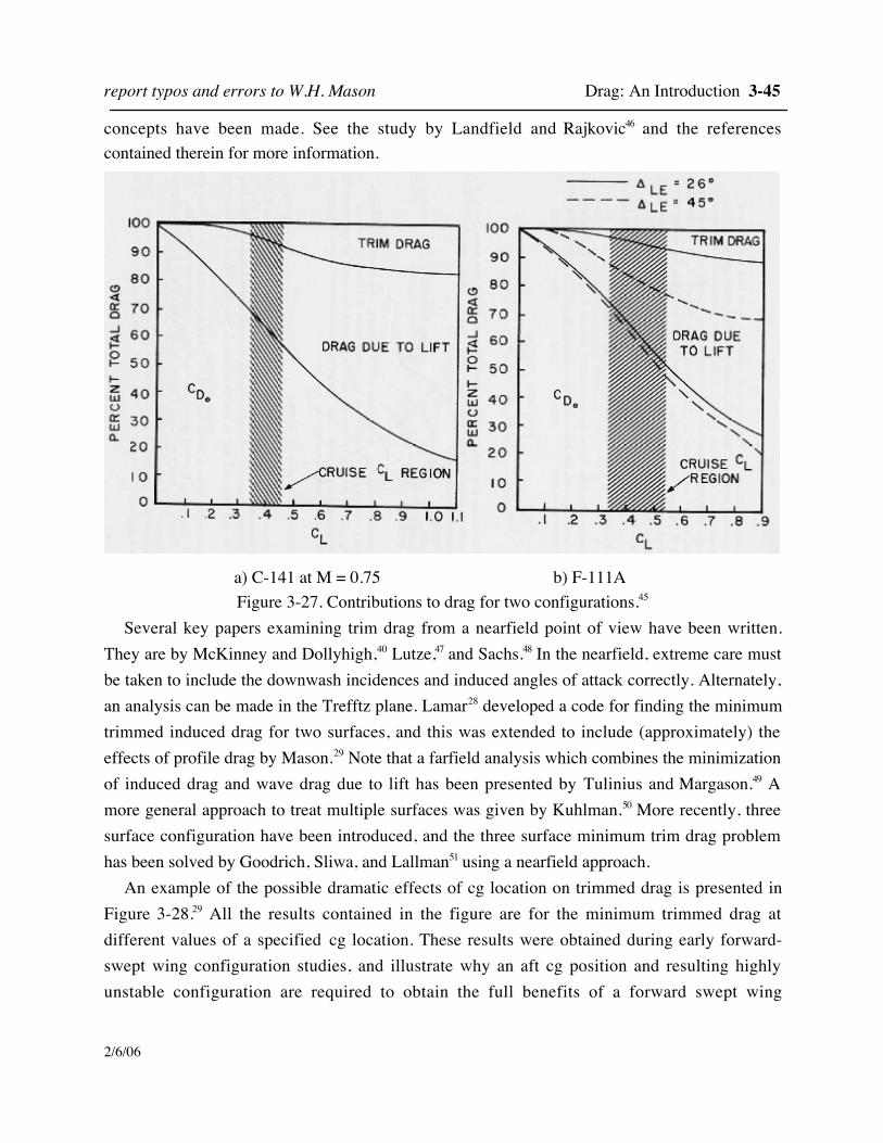
Trim drag is especially important for several specific classes of aircraft. Supersonic aircraftdemand special consideration because of the aerodynamic center shift from subsonic tosupersonic flight. To control trim drag as well as stability, fuel is transferred fore and aft betweensubsonic and supersonic flight to achieve proper balance on supersonic cruise aircraft. Variablesweep wing aircraft also have aerodynamic center locations that vary with wing sweep,potentially leading to high values of trim drag. Finally, maneuvering aircraft can suffer high trimdrag at high lift coefficients, severely limiting sustained turn performance. This was especiallytrue of the first generation of supersonic capable fighters. Examples of the contribution of trimdrag to the total drag are shown in Figure 3-27, taken from Nicolai.45
A more useful approach to the trim drag analysis is to consider the value of “trimmed drag”.In this approach it is difficult to define a specific trim drag value. The best way to assess the trimpenalty is to define the difference between the minimum drag attainable for the system and theminimum trimmed drag for a specified center of gravity position. This provides the designer witha measure of the drag penalty being paid for a particular center of gravity location. This approachalso demonstrates directly the connection between static margin and minimum trimmed drag.Different configuration concepts lead to different values of static margin to obtain minimumtrimmed lift. In general, for aft swept wings aft tail configurations, the minimum trimmed dragoccurs at a slightly unstable center of gravity (5-10%?), canard configurations have minimumtrim drag at slightly more unstable conditions (15%?), and forward swept wing canardconfigurations must be even more unstable to achieve minimum trimmed drag (the X-29 is about30-35% unstable). Many studies of these fundamental properties of various configuration
report typos and errors to W.H. Mason Drag: An Introduction 3-45
2/6/06
concepts have been made. See the study by Landfield and Rajkovic46 and the referencescontained therein for more information.
a) C-141 at M = 0.75 b) F-111AFigure 3-27. Contributions to drag for two configurations.45
Several key papers examining trim drag from a nearfield point of view have been written.They are by McKinney and Dollyhigh,40 Lutze,47 and Sachs.48 In the nearfield, extreme care mustbe taken to include the downwash incidences and induced angles of attack correctly. Alternately,an analysis can be made in the Trefftz plane. Lamar28 developed a code for finding the minimumtrimmed induced drag for two surfaces, and this was extended to include (approximately) theeffects of profile drag by Mason.29 Note that a farfield analysis which combines the minimizationof induced drag and wave drag due to lift has been presented by Tulinius and Margason.49 Amore general approach to treat multiple surfaces was given by Kuhlman.50 More recently, threesurface configuration have been introduced, and the three surface minimum trim drag problemhas been solved by Goodrich, Sliwa, and Lallman51 using a nearfield approach.
An example of the possible dramatic effects of cg location on trimmed drag is presented inFigure 3-28.29 All the results contained in the figure are for the minimum trimmed drag atdifferent values of a specified cg location. These results were obtained during early forward-swept wing configuration studies, and illustrate why an aft cg position and resulting highlyunstable configuration are required to obtain the full benefits of a forward swept wing
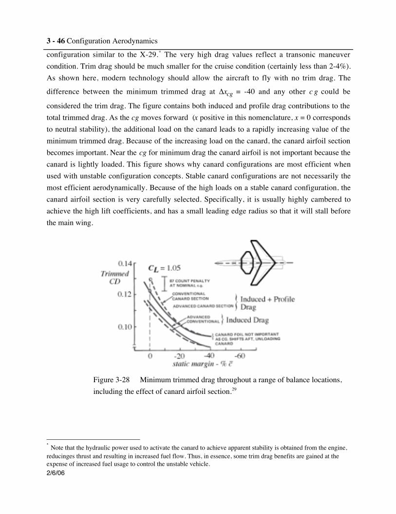
3 - 46 Configuration Aerodynamics
2/6/06
configuration similar to the X-29.* The very high drag values reflect a transonic maneuvercondition. Trim drag should be much smaller for the cruise condition (certainly less than 2-4%).As shown here, modern technology should allow the aircraft to fly with no trim drag. The
difference between the minimum trimmed drag at Δxcg = -40 and any other c g could be
considered the trim drag. The figure contains both induced and profile drag contributions to thetotal trimmed drag. As the cg moves forward (x positive in this nomenclature, x = 0 correspondsto neutral stability), the additional load on the canard leads to a rapidly increasing value of theminimum trimmed drag. Because of the increasing load on the canard, the canard airfoil sectionbecomes important. Near the cg for minimum drag the canard airfoil is not important because thecanard is lightly loaded. This figure shows why canard configurations are most efficient whenused with unstable configuration concepts. Stable canard configurations are not necessarily themost efficient aerodynamically. Because of the high loads on a stable canard configuration, thecanard airfoil section is very carefully selected. Specifically, it is usually highly cambered toachieve the high lift coefficients, and has a small leading edge radius so that it will stall beforethe main wing.
Figure 3-28 Minimum trimmed drag throughout a range of balance locations,including the effect of canard airfoil section.29
* Note that the hydraulic power used to activate the canard to achieve apparent stability is obtained from the engine,reducinges thrust and resulting in increased fuel flow. Thus, in essence, some trim drag benefits are gained at theexpense of increased fuel usage to control the unstable vehicle.
report typos and errors to W.H. Mason Drag: An Introduction 3-47
2/6/06
3.11 Current Issues for Drag Calculation Using Computational AerodynamicsBecause of the quest for reduced drag, and the difficulty in computing and measuring small
changes in drag, numerous disputes have arisen in aerodynamics. Confusion introduced by non-standard drag nomenclature also contributes to these spirited debates. One recent issue was theso-called sheared wing-tip drag reduction controversy. Here it was speculated that wing tipshaping could lead to span e’s greater than one for planar planforms.52 This conclusion arosebased on both computations and wind tunnel tests. Refined computational investigations,53
illustrating the need to study computational solution convergence carefully as shown elsewherein this text, resulted in the conclusion that e’s greater than one were not actually computed.However, it is clear that wing tip planform shaping can lead to improved aerodynamic efficiency.
Another area currently attracting attention is the search for more fundamental understandingof drag. These theories differ significantly from the accepted approach to drag. One key exampleis due to Yates.54
In addition to the efforts to reduce drag due to lift by tip shaping, use of winglets, tip sails,and canard configurations among others, significant efforts are being made to reduce skinfriction drag. They include efforts to obtain laminar flow through passive means (NLF), suction,or a combination known as hybrid natural laminar flow control. Turbulent friction reductiontechniques are also being developed. Riblets are perhaps the most well known means. A recentAIAA book reviews this area.55
3.12 Exercises1. Derive equations 3-7 and 3-8.2. Derive equations 3-31 and 3-32.3. Get a copy of LIDRAG and check it against the known values of the span e for an elliptic and
a triangular load distribution. How do your results compare?4. Use experimental results and show quantitatively that Fig. 3-11 is correct.5. Get a copy of FRICTION. Repeat the check case in the user’s manual. Then examine the skin
friction values in Table 3-1. Are they reasonable?6. Find the shape of the Karman ogive, the body with minimum wave drag for a given length and
base area.
3 - 48 Configuration Aerodynamics
2/6/06
References 1 Strang, W.J., and McKinlay, R.M., “Concorde in Service,” Aeronautical Journal, February,
1979.2 Bavitz, et al., “Configuration Development of Advanced Fighters,” Vol. 3, Concept Definition
and Validation, AFWAL-TR-3142, November 1980.3 Sloof, J.W., ed., “Technical Status Review on Drag Prediction and Analysis from
Computational Fluid Dynamics: State of the Art,” AGARD-AR-256, May 1988.4 Aerodynamic Drag, AGARD CP-124, April 1973.5 Aircraft Excrescence Drag. AGARD AG-264, 1981.6 Aircraft Drag Prediction and Reduction, AGARD-R-723, 1985.7 Special Course on Skin Friction Drag Reduction, AGARD R-786, March 19928 Covert, E.E., ed., Thrust and Drag: Its Prediction and Verification, AIAA, New York, 1985.9 Hoerner, S., Fluid Dynamic Drag, originally published by the author, and available from
Hoerner Fluid Dynamics, PO Box 21992, Bakersfield, CA 93390, now,http://members.aol.com/hfdy/home.htm
10 van Dam, C.P., “Recent experience with different methods of drag prediction,” Progress inAerospace Sciences, Vol. 35, 1999, pp. 751-798.
11 Torenbeek, E., Synthesis of Subsonic Airplane Design, Delft University Press, Delft, 1982.12 Whitford, R., Design for Air Combat, Jane’s London, 1987.13 Huenecke, K., Modern Combat Aircraft Design, Naval Institute Press, Annapolis, 1987.14 Haines, A.B., “Subsonic Aircraft Drag: An Appreciation of the Standards,” The Aeronautical
Journal of the Royal Aeronautical Society, Mar. 1968, pp. 253-266.15 Küchemann, D., The Aerodynamic Design of Aircraft, Pergamon Press, Oxford, 1978.16 Lynch, F.T., “Commercial Transports—Aerodynamic Design for Cruise Performance
Efficiency,” Transonic Aerodynamics, Nixon, D., ed., Progress in Astronautics andAeronautics, Vol. 181, AIAA New York, 1982.
17 Shevell, “Aerodynamic Bugs: Can CFD Spray Them Away?” AIAA Paper 85-4067, Oct.1985. Published in the Journal of Aircraft, Vol. 23, No. 8, August 1986, as “AerodynamicAnomalies: Can CFD Prevent or Correct Them?” pp. 641-649.
18 Rooney, E.C., “Thrust-Drag Accounting Methodology,” in Thrust and Drag: Its Predictionand Verification, Covert, E.E., ed., AIAA, New York, 1985.
19 Ashley, H., and Landahl, M., Aerodynamics of Wings and Bodies, Addison-Wesley, Reading,1965, sections 1.6, 6.6, 7.3 and 9.2. Now published by Dover.
20 Heaslet, M.A., and Lomax, H., “Supersonic and Transonic Small Perturbation Theory,” inGeneral Theory of High Speed Aerodynamics, W.R. Sears, ed., Princeton University Press,1954, sec. D,14: pp 221-229.
21 Liepman, H.W., and Roshko, A., Elements of Gasdynamics, John Wiley, New York, 1957, pp.235-239. Now published by Dover.
22 Harris, R.V., “An Analysis and Correlation of Aircraft Wave Drag,” NASA TM X-947, 1964.23 Kroo, Ilan, “Drag Due to Lift: Concepts for Prediction and Reduction,” Annual Review of
Fluid Mechanics, Vol. 33, 2001, pp. 587-617. Available for free electronically to Virginia Techstudents through the library web site.
24 Sears, W.R., “On Calculation of Induced Drag and Conditions Downstream of a Lifting

report typos and errors to W.H. Mason Drag: An Introduction 3-49
2/6/06
Wing,” Journal of Aircraft, Vol. 11, No. 3, March 1974, pp.191-192.
25 Thwaites, B., ed., Incompressible Aerodynamics, Oxford, 1960, pp. 454-457, 523-527. Nowpublished by Dover.
26 Mason, W.H., Mackenzie, D., Stern, M., Ballhaus, W.F., and Frick, J., “An AutomatedProcedure for Computing the Three Dimensional Transonic Flow over Wing-BodyCombinations, Including Viscous Effects,” AFFDL-TR-77-122, Feb. 1978.
27 Milne-Thomson, Theoretical Aerodynamics, Dover, New York, 1973, pp 218-21928 Lamar, J.E., “A Vortex Lattice Method for the Mean Camber Shapes of Trimmed Non-
Coplanar Planforms with Minimum Vortex Drag,” NASA TN D-8090, June, 1976.29 Mason, W.H., “Wing-Canard Aerodynamics at Transonic Speeds—Fundamental
Considerations on Minimum Drag Spanloads,” AIAA Paper 82-0097, Jan. 1982.30 Paterson, J.H., MacWilkenson, D.G., and Blackerby, W.T., “A Survey of Drag Prediction
Techniques Applicable to Subsonic and Transonic Aircraft Design,” in Aerodynamic Drag,AGARD CP 124, April 1973.
31 Jones, R.T. Wing Theory, Princeton University Press, Princeton, 1991.32 Whitcomb, R.T., “A Study of the Zero Lift Drag-Rise Characteristics of Wing-Body
Combinations near the Speed of Sound,” NACA Report 1273, 1956.33 Mendenhall, C., Delta Wings—Convair’s High Speed Planes of the Fifties and Sixties,
Motorbooks International, Osceola, WI, 1983.34 Anon., Aireviews Jet Fighters of the World Part 2, Kantosha Co. Ltd., Tokyo, 1965 (in
Japanese).35 Stuart, William G., “Northrop F-5 Case Study in Aircraft Design,” AIAA Professional Study
Series, Sept. 1978.36 Eminton, E., and Lord W.T., “Note on the Numerical Evaluation of the Wave Drag of Smooth
Slender Bodies Using Optimum Area Distributions for Minimum Wave Drag,” Journal of theRoyal Aeronautical Society, Vol. 60, Jan. 1956, pp. 61-63.
37 Robins, A.W., Dollyhigh, S.M., Beissner, F.L., Jr., Geiselhart, K., Martin, G.L., Shields, E.W.,Swanson, E.E., Coen, P.G., Morris, S.J., Jr., “Concept Development of a Mach 3.0 High-Speed Civil Transport,” NASA TM 4058
38 Hutchison, M., Unger, E., Mason, W.H., Grossman, B., and Haftka, R., “Variable-ComplexityAerodynamic Optimization of an HSCT Wing Using Structural Wing-Weight Equations,”AIAA Paper 92-0212, Jan. 1992.
39 Buckner, J.K., Benepe, D.B., Hill, D.W., “Aerodynamic Design Evolution of the F-16,” AIAAPaper 74-935, 1974.
40 McKinney, L.W., and Dollyhigh, S.M., “Some Trim Drag Considerations for ManeuveringAircraft,” Journal of Aircraft, Vol. 8, No. 8, Aug. 1971, pp.623-629.
41 Raymer, D.P., Aircraft Design: A Conceptual Approach, 3rd Ed., AIAA, Reston, 1999.42 Carlson,H.W., Mack, R.J., and Barger, R.L., “Estimation of Attainable Leading Edge Thrust
for Wings at Subsonic and Supersonic Speeds,” NASA TP 1500, 1979.43 Mann, M.J., and Carlson, H.W., “An Assessment of Current Methods for Drag-Due-To-Lift
Minimization at Supersonic Speeds,” AIAA Paper 91-3302, Sept. 1991.44 Mason,W.H., and DaForno, G., “Opportunities for Supersonic Performance Gains Through
Non-Linear Aerodynamics,” AIAA Paper 79-1527, July 1979.45 Nicolai, L.M., Fundamentals of Aircraft Design, METS, Xenia, 1975.46 Landfield, J.P., and Rajkovic, D., “Canard/Tail Comparison for an Advanced Variable-Sweep-
3 - 50 Configuration Aerodynamics
2/6/06
Wing Fighter,” AIAA Paper 84-2401, October 1984.
47 Lutze, F.H., “Trimmed Drag Considerations,” Journal of Aircraft, Vol. 14, No. 6, June 1977,pp.544-546.
48 Sachs, G., “Minimum Trimmed Drag and Optimum c.g. Position,” Journal of Aircraft, Vol.15, No. 8, Aug. 1978, pp. 456-459.
49 Tulinius, J.R., and Margason, R.J., “Aircraft Aerodynamic Design and Evaluation Methods,”AIAA Paper 76-15, Jan. 1976.
50 Kuhlman, J.M., “Higher Order Farfield Drag Minimization for a Subcritical Wing Design,”Journal of Aircraft, Vol. 17, No. 9, Sept. 1980, pp. 648-655.
51 Goodrich, K.H., Sliwa, S.M., and Lallman, F.J., “A Closed-Form Trim Solution YieldingMinimum Trim Drag for Airplanes with Multiple Longitudinal Control Effectors,” NASA TP2907, May 1989.
52 VanDam, C.P., “Induced-Drag Characteristics of Crescent-Moon-Shaped Wings,” Journal ofAircraft, Vol. 24, No. 2, Feb. 1987. pp. 115-119.
53 Smith, S.C., and Kroo, I.M., “A Closer Look at the Induced Drag of Crescent-Shaped Wings,”AIAA Paper 90-3063, Aug. 1990.
54 Yates, J.E., “Prediction of Drag and Lift: A Viscous/Thermodynamic Approach,” A.R.A.P.Report No. 651, Aug. 1990 (presented at an AIAA Short Course, Portland, Oregon, Aug. 23-24, 1990).
55 Bushnell, D.M., and Hefner, J.N., ed., Viscous Drag Reduction in Boundary Layers, AIAAProgress in Astronautics and Aeronautics Series, Vol. 123, AIAA, Washington, 1990.