3-d graphics and visualisation (part ii) - dcu
TRANSCRIPT

3-D Graphics and Visualisation (Part II)
EE563
Dr. Derek Molloy and Dr. Robert Sadleir

2

Contents
1 OpenGL - The Graphics Pipeline 51.1 Introduction . . . . . . . . . . . . . . . . . . . . . . . . . . . . . . . . . . . . 51.2 What is the OpenGL API? . . . . . . . . . . . . . . . . . . . . . . . . . . . 51.3 Introduction to OpenGL Programming . . . . . . . . . . . . . . . . . . . . . 9
1.3.1 OpenGL Primitives and Attributes . . . . . . . . . . . . . . . . . . . 91.3.2 OpenGL Full Source Code Example . . . . . . . . . . . . . . . . . . 141.3.3 OpenGL Colour . . . . . . . . . . . . . . . . . . . . . . . . . . . . . 161.3.4 Exercise: A Rotating Colour Solid . . . . . . . . . . . . . . . . . . . 171.3.5 OpenGL Viewing . . . . . . . . . . . . . . . . . . . . . . . . . . . . . 181.3.6 OpenGL Display Lists . . . . . . . . . . . . . . . . . . . . . . . . . . 241.3.7 OpenGL Stack . . . . . . . . . . . . . . . . . . . . . . . . . . . . . . 281.3.8 Input Events . . . . . . . . . . . . . . . . . . . . . . . . . . . . . . . 291.3.9 Double Buffering . . . . . . . . . . . . . . . . . . . . . . . . . . . . . 31
1.4 Some Math . . . . . . . . . . . . . . . . . . . . . . . . . . . . . . . . . . . . 321.4.1 3-D Math Notation . . . . . . . . . . . . . . . . . . . . . . . . . . . . 321.4.2 Vectors - Math summary . . . . . . . . . . . . . . . . . . . . . . . . 321.4.3 A Vector Class . . . . . . . . . . . . . . . . . . . . . . . . . . . . . . 371.4.4 Matrices . . . . . . . . . . . . . . . . . . . . . . . . . . . . . . . . . . 411.4.5 A Matrix Class . . . . . . . . . . . . . . . . . . . . . . . . . . . . . . 42
1.5 Transformations . . . . . . . . . . . . . . . . . . . . . . . . . . . . . . . . . 471.5.1 Translation . . . . . . . . . . . . . . . . . . . . . . . . . . . . . . . . 471.5.2 Rotation . . . . . . . . . . . . . . . . . . . . . . . . . . . . . . . . . . 481.5.3 Scaling . . . . . . . . . . . . . . . . . . . . . . . . . . . . . . . . . . 491.5.4 Shearing . . . . . . . . . . . . . . . . . . . . . . . . . . . . . . . . . . 491.5.5 Inverse Operations . . . . . . . . . . . . . . . . . . . . . . . . . . . . 501.5.6 Combination and Other Operations . . . . . . . . . . . . . . . . . . 501.5.7 The OpenGL Current Transformation Matrix (CTM) . . . . . . . . 501.5.8 Coordinate Spaces in the Graphics Pipeline . . . . . . . . . . . . . . 55
1.6 OpenGL Shading . . . . . . . . . . . . . . . . . . . . . . . . . . . . . . . . . 571.6.1 The Phong Model . . . . . . . . . . . . . . . . . . . . . . . . . . . . 581.6.2 Lambertian Surfaces . . . . . . . . . . . . . . . . . . . . . . . . . . . 601.6.3 The Normal Vector . . . . . . . . . . . . . . . . . . . . . . . . . . . . 611.6.4 Shading . . . . . . . . . . . . . . . . . . . . . . . . . . . . . . . . . . 631.6.5 Lighting . . . . . . . . . . . . . . . . . . . . . . . . . . . . . . . . . . 641.6.6 OpenGL code for Shading . . . . . . . . . . . . . . . . . . . . . . . . 65
2 Scene Graph Theory 672.1 Introduction . . . . . . . . . . . . . . . . . . . . . . . . . . . . . . . . . . . . 672.2 A Simple Scene Graph Implementation . . . . . . . . . . . . . . . . . . . . . 68
2.2.1 Traversing the Scene Graph . . . . . . . . . . . . . . . . . . . . . . . 702.2.2 Putting it Together: The Scene Graph with OpenGL . . . . . . . . . 742.2.3 Making it Better: The Scene Graph with OpenGL . . . . . . . . . . 79
2.3 Constructive Solid Geometry (CSG) . . . . . . . . . . . . . . . . . . . . . . 82
3

4 CONTENTS
2.4 Scene Graphs and Bounding Volume Hierarchies . . . . . . . . . . . . . . . 842.5 Space Subdivision Structures . . . . . . . . . . . . . . . . . . . . . . . . . . 85
2.5.1 Binary Space Partitioning Trees . . . . . . . . . . . . . . . . . . . . 852.6 Hidden Surface Removal . . . . . . . . . . . . . . . . . . . . . . . . . . . . . 88
2.6.1 The Painter’s Algorithm and BSP . . . . . . . . . . . . . . . . . . . 89
3 Real-Time 3D Computer Graphics Techniques 933.1 Introduction . . . . . . . . . . . . . . . . . . . . . . . . . . . . . . . . . . . . 933.2 Texture Mapping in OpenGL . . . . . . . . . . . . . . . . . . . . . . . . . . 93
3.2.1 Mipmapping . . . . . . . . . . . . . . . . . . . . . . . . . . . . . . . 983.3 Level of Detail (LOD) . . . . . . . . . . . . . . . . . . . . . . . . . . . . . . 983.4 Billboarding . . . . . . . . . . . . . . . . . . . . . . . . . . . . . . . . . . . . 1013.5 Mappings . . . . . . . . . . . . . . . . . . . . . . . . . . . . . . . . . . . . . 102
3.5.1 Bump Mapping . . . . . . . . . . . . . . . . . . . . . . . . . . . . . . 1023.5.2 Displacement Mapping . . . . . . . . . . . . . . . . . . . . . . . . . . 105
3.6 Shadows . . . . . . . . . . . . . . . . . . . . . . . . . . . . . . . . . . . . . . 1053.6.1 Algorithms for Computing Shadows . . . . . . . . . . . . . . . . . . 105
4 Appendices 1094.1 Installing Dev C++ . . . . . . . . . . . . . . . . . . . . . . . . . . . . . . . 1094.2 Exercise Solutions . . . . . . . . . . . . . . . . . . . . . . . . . . . . . . . . 109
4.2.1 Solution: A Rotating Colour Solid . . . . . . . . . . . . . . . . . . . 109

Chapter 1
OpenGL - The Graphics Pipeline
1.1 Introduction
The Graphics Pipeline is responsible for taking the description of a scene in 3-D spaceand mapping it to the view plane in a raster form, i.e. generally to the computer monitor.The most popular models of a graphics pipeline with an extensive API are Java3D andOpenGL.
1.2 What is the OpenGL API?
OpenGL is defined simply as ‘a software interface to graphics hardware”, but this does notdo justice to the true capability of this technology; it is an extremely fast graphics librarythat provides with all the functionality we require to model in 3-D. OpenGL is intendedfor use with graphics hardware, but there are software versions of OpenGL available - inparticular the Microsoft version; however, these days almost all personal computers aresupplied with a 3-D graphics card that contains a hardware implementation of OpenGL.Indeed, OpenGL works well in hiding the complexities involved with different 3D graphicaccelerators and their processing capabilities, which are supplied from different vendors1.The processing capability of OpenGL is supplied by a graphics pipeline, known as theOpenGL State Machine, which is illustrated in 1.1 and 1.2.
There are several 3-D graphic Application Programming Interfaces (APIs) available,such as OpenGL, Direct3D and Java3D. We have discussed Java3D earlier in this mod-ule, and now we are discussing the lower-level OpenGL API: We could have examinedthe Direct3D API, but it is a Microsoft Technology, tied to the Windows OS. OpenGL ismaintained by Silicon Graphics Ltd. (SGI) and provides a standard specification defininga cross-platform API for writing 3-D graphic applications. OpenGL is more commonlyused in 3-D Visualisation applications, whereas Direct3D is more commonly used in com-puter gaming applications. As mentioned, OpenGL is a low-level API, which requires theprogrammer to supply the exact steps to render a scene. This makes the generation ofscenes much more difficult than Java3D where we only had to describe the scene, butit makes it possible for us to create novel rendering algorithms or to configure how thepipeline processes the primitives that we specify.
OpenGL provides us with the functionality to specify the objects, cameras, light sourcesand materials that we need to create 3-D scenes. OpenGL allows us to create objects byusing points, line segments, triangles and polygons... in particular, we create objectsthrough lists of vertices. The following listing allows us to create a simple triangle in thexy plane (i.e. with z = 0 for every vertex):
0 glBegin(GL POLYGON);
1The best known vendors are probably nVidia (www.nvidia.com) and ATI technologies (www.ati.com)- now owned by AMD
5

6 CHAPTER 1. OPENGL - THE GRAPHICS PIPELINE
glVertex3f(0.0 f , 0.0f , 0.0f );glVertex3f(0.0 f , 1.0f , 0.0f );glVertex3f(1.0 f , 0.0f , 0.0f );
glEnd();
The function glBegin() specifies the type of shape that the vertices define. Each callto the glVertex() function gives the x, y and z position of the vertex. In this case weare creating a GL POLYGON but we could change this to GL POINTS to specify 3 points, orGL LINE STRIP to specify two connected lines. So, in the example above, we could haveused glVertex2f() instead, as the z-component is 0 in each case. This is typical of thesyntax used in OpenGL.
The glVertex*() function allows us many different functions to specify a vertex in3-D space; we can use two, three and even four dimensional spaces in OpenGL. In thisfunction the * can be replaced by any of the numbers 2, 3 or 4 and the particular typeof the value of the vertex, e.g. float(f), double(d), integer(i) or pointer(v): So,glVertex2i(10,20) would specify that we are creating a vertex using two integer valuesat (10, 20). We generally use the OpenGL types that are defined in the OpenGL headerfiles, such as: #define GLfloat float. This allows flexibility for implementations wherewe might want to change floats into doubles without affecting the code already written.Note that OpenGL functions all begin with the letters gl.
We can use arrays of points, using the following syntax:
0 GLfloat vertices [3][3] = {{0.0f, 1.0f , 0.0f},{0.87f , −0.5f, 0.0f}, {−0.87f, −0.5f, 0.0f}};
// ...glBegin (GL TRIANGLES);
for(int i=0; i<3; i++)5 {
glVertex3fv( vertices [ i ]);}
glEnd ();// ...
For a full source example see: Example1aThe OpenGL user API provides us with a set of resources to help us in the development
of our applications:
• OpenGL Utility Library (GLU) - This library provides us with a set of functionsfor drawing objects (such as spheres), manipulating textures, creation of standardviews, NURBS surfaces etc.; functions that are common across many applications.The prefix for functions of this library is glu, not gl.
• OpenGL Utility Toolkit (GLUT) - This library provides us with functionality re-lated to the windowing system on the current platform, for creating windows, createmenus, interaction with the mouse, draw objects, display text etc. The prefix forfunctions of this library is glut. The GLUT library is available from Nate Robins’web site: http://www.xmission.com/~nate/glut.html.
To include these libraries, we can use #include<GL/glut.h> for example. Figure 1.3illustrates a simplified OpenGL Windows pipeline.
OpenGL Resources
The following are a list of the most important OpenGL references for this module:
• The OpenGL Red Book - This book is the programming guide for OpenGL. It isdesigned to explain OpenGL functionality and to give examples of its use. The RedBook is currently in its fifth edition, which covers OpenGL Version 2, but here is an

1.2. WHAT IS THE OPENGL API? 7
TexCoord1
TexCoord2
TexCoord3
TexCoord4
Color3
Color4Convert
RGBA to float
Index Convertindex to float
CurrentTexture
Coordinates
CurrentRGBAColor
CurrentColorIndex
CurrentNormal
Normal3
Vertex2RasterPos2
Vertex3RasterPos3
Vertex4RasterPos4
bM
M*b
Model ViewMatrixStack
OBJECTCOORDINATES
EYECOORDINATES
M
MatrixControl
MatrixModePushMatrix
PopMatrix
LoadIdentityLoadMatrix
NM
M*N
MatrixGenerators
TranslateScale
RotateFrustum
Ortho
EdgeFlagCurrent
EdgeFlag
CurrentRaster
Position
CullFace
PolygonCulling
PolygonMode
PolygonMode
PointSize
Enable/Disable(Antialiasing/Stipple)
UnpackPixels
Bitmap
DrawPixels
TexImage
PolygonStipple
PixelTransfer
PixelTransfer
PixelStore
PackPixels
ReadPixels
MultMatrix
bM
M*b Normalize
Enable/Disable
TexGenOBJECT_LINEAR
TexGenEYE_LINEAR
TexGenSPHERE_MAP
Enable/Disable
bA
A*b
TextureMatrixStack
MaterialParameters
Control
ColorMaterialMaterial
Enable/Disable
LightParameters
RGBA Lighting Equation
Color Index Lighting Equation
MaterialParameters
Light ModelParameters
LightEnable/Disable
LightModel
MM−T
Enable/Disable
Clamp to[0,1]
Mask to
[0,2n−1]
PrimitiveAssembly
Begin/End
TexGen
(Lighting)
EvalMeshEvalPoint
EvalCoord
MapGrid
Map
GridApplication
MapEvaluation
DivideVertex
Coordinatesbyw
ApplyViewport
DepthRangeViewport
Flatshading
POINTSRASTER POS.
LINESEGMENTS
POLYGONS
ShadeModel
LineClipping
PolygonClipping
PointCulling
ClipPlanes
ClipPlane
Mb
b
b
(VertexOnly)
LineView Volume
Clipping
PolygonView Volume
Clipping
PointView Volume
Culling
M*b
ProjectionMatrixStack
MM−Tb
b
FeedbackEncoding
FeedbackBuffer
PassThrough
SelectionControl
SelectBuffer
RenderMode
EvaluatorControl
RectangleGeneration
Rect
M*b
M*b
FrontFace
FrontFace
LineStipple
Enable/Disable(Antialiasing)
PixelMap
SelectionNameStack
SelectionEncoding
InitNames
PopNamePushName
LoadName
Notes:1. Commands (and constants) are shown without the
gl (or GL_) prefix.2. The following commands do not appear in this diagram: glAccum, glClearAccum, glHint, display list commands, texture object commands, commands for obtaining OpenGL state (glGet commands and glIsEnabled), and
glPushAttrib and glPopAttrib. Utility library routines are not shown.3. After their exectution, glDrawArrays and
glDrawElements leave affected current values indeterminate.4. This diagram is schematic; it may not directly correspond to any actual OpenGL implementation.
Convertnormal coords
to float
Enable/Disable
TexSubImage
PolygonOffset
LineWidth
Enable/Disable(Antialiasing)
EdgeFlagPointer
TexCoordPointer
ColorPointer
IndexPointer
NormalPointer
VertexPointer
InterLeavedArrays
EnableClientStateDisableClientState
DrawElements
ArrayElement
VertexArray
Control
t 0
r 0
q 1
A 1
z 0
w 1
DrawArrays
Figure 1.1: A schematic diagram of the OpenGL State Machine LHS c©Silicon GraphicsLtd.

8 CHAPTER 1. OPENGL - THE GRAPHICS PIPELINE
The OpenGL MachineR
The OpenGL ? graphics system diagram, Version 1.1. Copyright ? 1996 Silicon Graphics, Inc. All rights reserved.
PolygonRasterization
LineSegment
Rasterization
PointRasterization
BitmapRasterization
PixelRasterization
PointSize
Enable/Disable(Antialiasing/Stipple)
PixelZoom
TexelGeneration
TextureMemory
TexParameter
TextureApplication
Fog
TexEnv FogEnable/Disable Enable/Disable
Masking
ColorMaskIndexMask
DepthMaskStencilMask
Coverage(antialiasing)Application
PixelOwnership
Test
AlphaTest
(RGBA only)
ScissorTest
StencilTest
DepthBufferTest
ClearValues
ClearControl
Clear
ClearColorClearIndexClearDepth
ClearStencil
Blending(RGBA only)
Dithering Logic Op
Frame Buffer
Scissor AlphaFuncStencilOp
StencilFunc
Enable/DisableEnable/Disable Enable/Disable Enable/Disable Enable/Disable Enable/Disable Enable/Disable
Enable/Disable
DepthFunc BlendFunc LogicOp
Frame BufferControl
DrawBuffer
ReadbackControl
ReadBuffer
Masking
LineStipple
Enable/Disable(Antialiasing)
CopyPixelsCopyTexImage
CopyTexSubImage
PolygonOffset
LineWidth
Enable/Disable(Antialiasing)
Key to OpenGL Operations
stnemgarFsevitimirP
Vertices
Feedback&
Selection
InputConversion
&CurrentValues
Texture CoordinateGeneration
Evaluators&
Vertex Arrays
Lighting
MatrixControl
Clipping, Perspective,and
Viewport Application Rasteriz−ation Texturing,
Fog,and
Antialiasing
Per−Fragment Operations
Frame Buffer&
Frame Buffer ControlPixels
Figure 1.2: A schematic diagram of the OpenGL State Machine RHS c©Silicon GraphicsLtd.

1.3. INTRODUCTION TO OPENGL PROGRAMMING 9
C/C++OpenGL
Application
GL (Core)Library
GLU (Utility)Library
GLUT/MFCLibrary
Win32
Graphics HardwareFrame Buffer
Figure 1.3: The Simplified OpenGL Windows Pipeline.
Geometric Pipeline
OpenGLApplication
Transform
PixelOperations
Clipping Projection
FrameBufferPixel Pipeline
Figure 1.4: A simplified OpenGL pipeline.
older version of the book in resourcesredbook.pdf and associated examples in resourcesredbookexamples.zip.
• The OpenGL Blue Book - This book is the reference guide for OpenGL. It is designedto document all the functionality of OpenGL. It currently covers version 1.4 ofOpenGL, but an old version is available here in resourcesbluebook.pdf, which covers OpenGL version 1.0.
• OpenGL Specification Version 2.1 - The OpenGL specification 2.1 was released inAugust 2006 and it describes the latest features of OpenGL. The most up-to-datespecification is available at resourcesOpenGLSpecificationVersion2 1.pdf.
1.3 Introduction to OpenGL Programming
1.3.1 OpenGL Primitives and Attributes
The core OpenGL library supports a relatively small set of geometric primitives (suchas points, lines, polygons, curves and surfaces) and raster primitives (such as arrays ofpixels). Figure 1.4 (see 1.1 and 1.2 for the full diagram) illustrates the series of geometricoperations which are used to see if a primitive appears on the screen (frame buffer). Thetransform block allows 2-D/3-D geometric primitives to be rotated or translated. Becauseraster objects do not have geometric properties, they cannot be manipulated in the sameway and so follow a parallel path through the pipeline.
As discussed previously, basic OpenGL geometric primitives are created using thefollowing code:
0 glBegin(<type>);glVertex ∗(...);...

10 CHAPTER 1. OPENGL - THE GRAPHICS PIPELINE
(a) GL_POINTS (b) GL_LINES (c) GL_LINE_LOOP (d) GL_LINE_STRIP
P0
P7
P1
P2
P3
P4
P5
P6
P0
P7
P1
P2
P3
P4
P5
P6
P0
P7
P1
P2
P3
P4
P5
P6
P0
P7
P1
P2
P3
P4
P5
P6
Figure 1.5: OpenGL Line Based Primitives.
(a) Simple Convex
P1
P2
(b) Simple Concave
P1
P2
(c) Complex (non-simple)
Figure 1.6: Displaying a polygon correctly (a) simple convex shapes (b) concave shapes(c) a non-simple polygon
glVertex ∗(...);glEnd();
where ∗ defines the particular glVertex function to call, and where <type> is one ofthe following (see figure 1.5(a)-(d)) in the case of line based primitives:
• GL POINTS - Each vertex is displayed as a point, with a size of at least one pixel.
• GL LINES - Each vertex pair are used as the start and end point, thus creating a line.
• GL LINE LOOP - Each vertex is used as the end point to create a line, using theprevious vertex as the start point (except P0). The line loop connects the last pointto the first point, thus creating a loop.
• GL LINE STRIP - Each vertex is used as the end point to create a line, using theprevious vertex as the start point (except P0).
When we are creating objects that are constructed like line loops (see figure 1.5(c)),but are filled in some way, we use the term polygon. Polygons are the fundamental build-ing blocks of complex models, in that these models are constructed from thousands ofpolygons.
For a polygon to be displayed correctly it must be (see figure 1.6):
• simple - the polygon should have a well-defined interior region. Lines connecting thevertices of the polygon should not cross.
• convex - an object is convex if all points on the object, or its boundary may beconnected without leaving the boundary of the object2.
2A set in Euclidean space R is a convex set if it contains all the line segments connecting any pair of

1.3. INTRODUCTION TO OPENGL PROGRAMMING 11
(a) GL_POLYGON (b) GL_QUADS (c) GL_TRIANGLES
P0
P7
P1
P2
P3
P4
P5
P6
P0
P7
P1
P2
P3
P4
P5
P6
P0
P7
P1
P2
P3
P4
P5
P6
(d) GL_TRIANGLE_STRIP
P0
P7P1
P2
P3
P4
P5
P6
(e) GL_QUAD_STRIP
P0
P7P1
P2
P3
P4
P5
P6
(f ) GL_TRIANGLE_FAN
P0 P7
P1
P2 P3 P4 P5
P6
Figure 1.7: OpenGL Polygon Based Primitives.
• flat - for a 3-D polygon all points of the polygon must lie on the same plane. If weare using triangles to represent polygons then this is not an issue.
We can use the same segment of code to create polygon objects:
0 glBegin(<type>)glVertex ∗(...);...glVertex ∗(...);
glEnd();
where ∗ defines the particular glVertex function to call, and where <type> is one ofthe following (see figure 1.7(a)-(f)) in the case of polygon based primitives:
• GL POLYGON - Each successive vertex defines a line segment, with the final vertexconnected to the first vertex. The interior of the polygon is filled according to thecurrent OpenGL state. If we wish we can use the glPolygonMode() function todisplay the edges or points of the vertices, instead of filling the polygon.
• GL TRIANGLES and GL QUADS - For the purpose of efficiency, it is possible to usesuccessive groups of either 3 or 4 vertices to create complex objects.
• GL TRIANGLE STRIP, GL QUAD STRIP and GL TRIANGLE FAN - When complex objectsare being constructed that share vertices and edges, these types are particularlyefficient at where each additional vertex is combined with the two previous verticesin the case of a triangle strip array; each new pair of vertices combine with theprevious two vertices for the quad strip array; and using one fixed point and eachsubsequent vertex in the case of a triangle fan array.
Here is an example of using these basic primitives to create more complex objects.The easy way to do this is to use the fact that GLUT already provides a set of complexprimitives such as a sphere. Example1b provides the source code project for an example ofdrawing a sphere using GLUT, and a screen capture of this application is shown in figure1.8.
To use this example you must complete the following steps:
its points. If the set does not contain all the line segments, it is called concave. The convex hull is the setof points that we get by stretching a tight-fitting surface over the object (like an elastic band in the 2-Dcase). It is the smallest convex object that includes the the set of points.

12 CHAPTER 1. OPENGL - THE GRAPHICS PIPELINE
Figure 1.8: Using OpenGL GLUT to draw a sphere.
• Download the GLUT library from http://www.xmission.com/~nate/glut.html
• Place the GLUT.h file in the DevC++ header file “GL” directory (i.e. where GL.his located)
• Place the .lib file in the DevC++ library directory.
• Place the GLUT32.dll file in the windows SYSTEM32 directory.
• In DevC++ Project −→ Project Options −→ press on “Parameters” and add thefollowing libraries to your Linker: -lglut32 -lwinmm -lgdi32
• In DevC++ you seem to have to add a line #define GLUT DISABLE ATEXIT HACK toyour code to get it to work correctly.
We can then very simply create a red sphere by using the code:
0 // Set the current OpenGL color to redglColor4f (1.0, 0.0, 0.0, 1.0);// Draw a wire sphereglutWireSphere(0.95, 10, 10);
If we wish to do this the hard way! In this example we will approximate a sphere. Wecan do this very efficiently by using a set of polygons defined by lines of longitude, usingeither triangle strips of quad strips. A sphere can be described by the following equations:
x(θ, φ) = r sin θ cos φ
y(θ, φ) = r cos θ cos φ
z(θ, φ) = r sinφ
where −180 ≤ θ ≤ +180 and −90 ≤ φ ≤ +90. In this case when φ is fixed, we can drawcircles of constant latitude by varying θ (the Earth’s equator is a line of latitude). In ourcode we will only vary −80 ≤ φ ≤ +80, so that the top and bottom (poles) of the spherecan be closed more accurately using a triangle fan. Figure 1.9(a) illustrates the approachto be taken where we will use GL QUAD STRIPs to fill in the largest area of the sphere andGL TRIANGLE FANs to fill in the top and bottom of the sphere, ensuring that our spherebegins and ends with a single point. To get OpenGL to display all of the lines in the sphereit is necessary to set the mode to: glPolygonMode(GL FRONT AND BACK, GL LINE); Thesource code for this example can be found in the Example1c directory.
Here is the implementation of the code for figure 1.9(b), where both ends of thesphere have not yet been closed. For this example we call the method by the call:

1.3. INTRODUCTION TO OPENGL PROGRAMMING 13
0
1
2
3
4
5
GL_QUAD_STRIP
GL_TRIANGLE_FAN
(a) (b) (c)
Figure 1.9: Drawing a sphere manually using the OpenGL core functionality. (a) illustratesthe approach taken (b) shows a screen grab with the ends not closed and (c) shows a screengrab with the ends closed
drawGLSphere(0.75f, 10.0f); where the first arguments specifies the radius of thesphere and the second specifies the number of degrees to use for each component polygon,i.e. a larger number gives a lower resolution sphere mesh. Remember that the standardtrigonometric functions in C++ work in radians, so while we can specify the behaviour ofour sphere in degrees, we must do the calculations in radians.
0 void drawGLSphere(GLfloat radius, GLfloat step){
GLfloat x,y,z, c = 3.14159f/180.0f;for (GLfloat phi=−80.0f; phi<80.0; phi+=step){
5 GLfloat phi rad = c ∗ phi;GLfloat phi rad end = c ∗ (phi+step);glBegin(GL QUAD STRIP);for (GLfloat theta=−180.0f; theta<=180.0f; theta+=step){
10 GLfloat theta rad = c ∗ theta;x = radius ∗ sin(theta rad)∗cos(phi rad);y = radius ∗ cos(theta rad)∗cos(phi rad);z = radius ∗ sin(phi rad);glVertex3f(x,y,z );
15 x = radius ∗ sin(theta rad)∗cos(phi rad end);y = radius ∗ cos(theta rad)∗cos(phi rad end);z = radius ∗ sin(phi rad end);glVertex3f(x,y,z );
}20 glEnd();
}}
To close the sphere at the top and bottom as in figure 1.9(b) it is necessary to addsome more code within the same function:
0 // Close one endGLfloat closeRing rad = c ∗ 80.0;glBegin(GL TRIANGLE FAN);glVertex3f(0.0 f , 0.0f , −radius);z = radius ∗ −sin(closeRing rad);
5 for(GLfloat theta=−180.0f; theta<=180.0f; theta+=step){
GLfloat theta rad = c ∗ theta;x = radius ∗ sin(theta rad) ∗ cos(closeRing rad);y = radius ∗ cos(theta rad) ∗ cos(closeRing rad);
14 CHAPTER 1. OPENGL - THE GRAPHICS PIPELINE
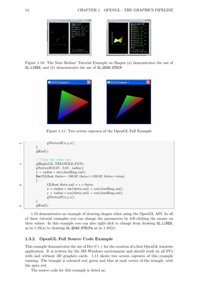
Figure 1.10: The Nate Robins’ Tutorial Example on Shapes (a) demonstrates the use ofGL LINES, and (b) demonstrates the use of GL QUAD STRIP
.
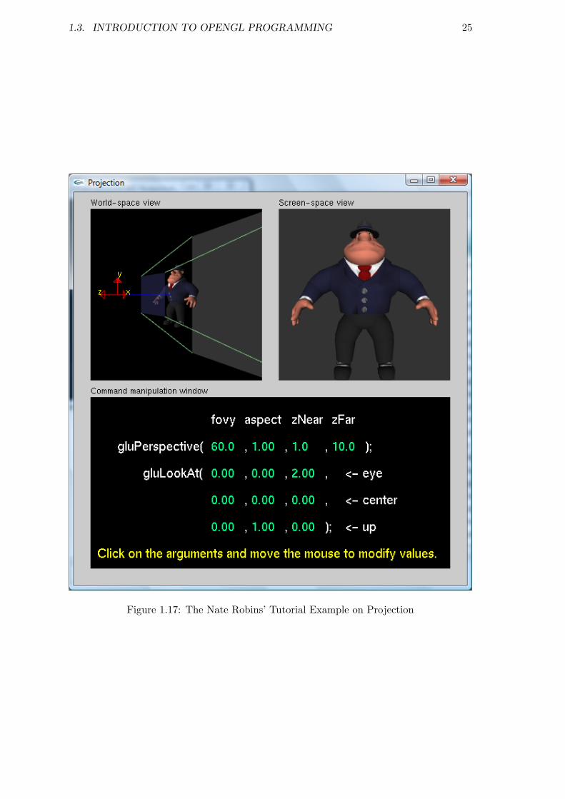
Figure 1.11: Two screen captures of the OpenGL Full Example
10 glVertex3f(x,y,z );}glEnd();
// Close the other end15 glBegin(GL TRIANGLE FAN);
glVertex3f(0.0 f , 0.0f , radius );z = radius ∗ sin(closeRing rad);for(GLfloat theta=−180.0f; theta<=180.0f; theta+=step){
20 GLfloat theta rad = c ∗ theta;x = radius ∗ sin(theta rad) ∗ cos(closeRing rad);y = radius ∗ cos(theta rad) ∗ cos(closeRing rad);glVertex3f(x,y,z );
}25 glEnd();
1.10 demonstrates an example of drawing shapes when using the OpenGL API. In allof these tutorial examples you can change the parameters by left-clicking the mouse ontheir values. In this example you can also right-click to change from drawing GL LINES,as in 1.10(a) to drawing GL QUAD STRIPs as in 1.10(b).
1.3.2 OpenGL Full Source Code Example
This example demonstrates the use of Dev C++ for the creation of a first OpenGL windowsapplication. It is written for the MS Windows environment and should work on all PCswith and without 3D graphics cards. 1.11 shows two screen captures of this examplerunning. The triangle is coloured red, green and blue at each vertex of the triangle, withthe apex red.
The source code for this example is listed as:

1.3. INTRODUCTION TO OPENGL PROGRAMMING 15
0 /∗∗∗∗∗∗∗∗∗∗∗∗∗∗∗∗∗∗∗∗∗∗∗∗∗∗∗∗∗∗∗∗∗∗∗∗∗∗∗∗∗∗∗ EE563 Example Project 1∗ by: Derek Molloy∗ based on the DevC++ OpenGL template∗
5 ∗∗∗∗∗∗∗∗∗∗∗∗∗∗∗∗∗∗∗∗∗∗∗∗∗∗∗∗∗∗∗∗∗∗∗∗∗∗∗∗∗∗/
#include <windows.h> // Header File For Windows#include <gl\gl.h> // Header File For The OpenGL32 Library#include <gl\glu.h> // Header File For The GLu32 Library
10HDC hDC=NULL; // Private GDI Device ContextHGLRC hRC=NULL; // Permanent Rendering ContextHWND hWnd=NULL; // Holds Our Window HandleHINSTANCE hInstance; // Holds The Instance Of The Application
15// Function Declarations
LRESULT CALLBACK WndProc (HWND hWnd, UINT message, WPARAM wParam,LPARAM lParam);
20 void enableOpenGL (HWND hWnd, HDC ∗hDC, HGLRC ∗hRC);int initGL(GLvoid);int drawGLScene(float theta);void disableOpenGL (HWND hWnd, HDC hDC, HGLRC hRC);
25 // WinMain − the starting point of our application
int WINAPI WinMain (HINSTANCE hInst, HINSTANCE hPrevInstance,LPSTR lpCmdLine, int iCmdShow)
{30 WNDCLASS wc;
HGLRC hRC;hInstance = hInst;MSG msg;BOOL bQuit = FALSE;
35 float theta = 0.0f;
// register window classwc.style = CS OWNDC;wc.lpfnWndProc = WndProc;
40 wc.cbClsExtra = 0;wc.cbWndExtra = 0;wc.hInstance = hInstance;wc.hIcon = LoadIcon (NULL, IDI APPLICATION);wc.hCursor = LoadCursor (NULL, IDC ARROW);
45 wc.hbrBackground = (HBRUSH) GetStockObject (BLACK BRUSH);wc.lpszMenuName = NULL;wc.lpszClassName = ”EE553GLExample”;RegisterClass (&wc);
50 // create main windowhWnd = CreateWindow (”EE553GLExample”, ”EE553 Example 1”,
WS CAPTION | WS POPUPWINDOW | WS VISIBLE,0, 0, 256, 256,NULL, NULL, hInstance, NULL);
55// enable OpenGL for the windowenableOpenGL (hWnd, &hDC, &hRC);initGL();
60 // program main loopwhile (!bQuit){
// check for messagesif (PeekMessage (&msg, NULL, 0, 0, PM REMOVE))
65 {// handle or dispatch messagesif (msg.message == WM QUIT){
bQuit = TRUE;70 }
else{
TranslateMessage (&msg);DispatchMessage (&msg);
75 }}else{
drawGLScene(theta);80 SwapBuffers (hDC);
theta += 1.0f;Sleep (1);
}}
85 // shutdown OpenGLdisableOpenGL (hWnd, hDC, hRC);// destroy the window explicitlyDestroyWindow (hWnd);return msg.wParam;
90 }
// Window Callback Process
95 LRESULT CALLBACK WndProc(HWND hWnd, UINT message, WPARAM wParam, LPARAM lParam){
switch (message){
case WM CREATE:100 return 0;
case WM CLOSE:PostQuitMessage (0);

16 CHAPTER 1. OPENGL - THE GRAPHICS PIPELINE
return 0;case WM DESTROY:
105 return 0;case WM KEYDOWN:
switch (wParam){case VK ESCAPE:
110 PostQuitMessage(0);return 0;
}return 0;
default:115 return DefWindowProc (hWnd, message, wParam, lParam);
}}
120 //Enable OpenGL
void enableOpenGL (HWND hWnd, HDC ∗hDC, HGLRC ∗hRC){
PIXELFORMATDESCRIPTOR pfd;125 int iFormat;
// get the device context (DC)∗hDC = GetDC (hWnd);
130 // set the pixel format for the DCZeroMemory (&pfd, sizeof (pfd));pfd.nSize = sizeof (pfd);pfd.nVersion = 1;pfd.dwFlags = PFD DRAW TO WINDOW | PFD SUPPORT OPENGL | PFD DOUBLEBUFFER;
135 pfd.iPixelType = PFD TYPE RGBA;pfd.cColorBits = 24;pfd.cDepthBits = 16;pfd.iLayerType = PFD MAIN PLANE;iFormat = ChoosePixelFormat (∗hDC, &pfd);
140 SetPixelFormat (∗hDC, iFormat, &pfd);
// create and enable the render context (RC)∗hRC = wglCreateContext( ∗hDC );wglMakeCurrent( ∗hDC, ∗hRC );
145 }
// Setup our GL Sceneint initGL(GLvoid){
150 glShadeModel(GL SMOOTH); // Enable Smooth ShadingglClearColor(0.0f , 0.0f , 0.0f , 0.5f );// Black BackgroundglClearDepth(1.0f); // Depth Buffer SetupglEnable(GL DEPTH TEST); // Enables Depth TestingglDepthFunc(GL LEQUAL); // The Type Of Depth Testing To Do
155 glHint(GL PERSPECTIVE CORRECTION HINT,GL NICEST); // Really Nice Perspective Calculations
return TRUE; // Initialization Went OK}
160 // Called to update the scene − give us the animationint drawGLScene(float theta) // Draw the scene;{ // theta is amount to rotate
glClear (GL COLOR BUFFER BIT | GL DEPTH BUFFER BIT); // Clear Screen165 glLoadIdentity();
glPushMatrix ();glRotatef (theta, 1.0f , 1.0f , 0.0f ); // Rotate theta around the xy−axisglBegin (GL TRIANGLES); // Drawing Using Triangles
glColor3f (1.0 f , 0.0f , 0.0f ); glVertex2f (0.0 f , 1.0f );170 glColor3f (0.0 f , 1.0f , 0.0f ); glVertex2f (0.87f , −0.5f);
glColor3f (0.0 f , 0.0f , 1.0f ); glVertex2f (−0.87f, −0.5f);glEnd ();glPopMatrix ();
return TRUE; // Keep Going175 }
// Disable OpenGLvoid disableOpenGL (HWND hWnd, HDC hDC, HGLRC hRC){
180 wglMakeCurrent (NULL, NULL);wglDeleteContext (hRC);ReleaseDC (hWnd, hDC);
}
1.3.3 OpenGL Colour
There are two colour models used in OpenGL; the RGB Colour Model and the IndexedColour Model. OpenGL provides us with a fairly simple mechanism for specifying colourdirectly by providing the red, green and blue values directly. When using 24-bit colour(224 = 16.7M colours) we specify our colour components as values between 0.0 and 1.0,using functions such as:
0 glColor3f(0.0 f , 0.0f , 1.0f ); // (R, G, B)

1.3. INTRODUCTION TO OPENGL PROGRAMMING 17
(a) (b) (c)
Green
Blue
Red
Yellow
White
Red
Magenta
Cyan
Blue
Green
Black
Figure 1.12: The Colour Cube Exercise (a) Colour Cube ;(b),(c) Screen Grabs of mysolution.
which sets the current drawing colour to blue. The drawing colour will remain as blue untilwe change the colour again. OpenGL also provides support for transparency (opacity),which can be used for transparent models, image blending or for effects such as fog. Thefunction takes a fourth parameter which specifies the level of opacity, which can vary from0.0 (fully transparent) to 1.0 (fully opaque).
0 glColor4f(0.0 f , 0.0f , 1.0f , 1.0f ); // (R, G, B, A)
which will give us a fully opaque blue. If we wish to change the background colour we canuse the function:
0 glClearColor(1.0f , 1.0f , 1.0f , 1.0f ); // (R, G, B, A)
which will result in a white clearing colour. OpenGL also has support for indexed colour,by providing a user-defined colour-lookup table that is of size 2n, which contains 3 columns,one for each of R,G, and B. If the bit level for each of R,G and B is 8-bits then the usercan choose 2n individual colours out of the 16.7M possibilities, creating a palette. Whenyou are in indexed colour mode you can select the current colour from the palette, byusing:
0 glIndexi ();
The indexed colour model is not so important any more due to the vast capabilities oftodays’ graphics cards.
1.3.4 Exercise: A Rotating Colour Solid
Write the code to generate a rotating colour solid which demonstrates the range of RGBcolours that has a variable diameter. Please use the structure as illustrated in figure 1.12,where (a) illustrates the colour cube, and (b),(c) show screen grabs of my solution.
Please note that OpenGL uses variants of bilinear interpolation to generate the coloursbetween the vertices. Therefore, as in the previous triangle example it is possible to specifycolours on a vertex-by-vertex basis and allow OpenGL to do the colour mixing over thepolygons.
You should try to write this code as efficiently as possible. You should be able tomodify previous examples to generate the cube, but you should look in particular at theglVertex3fv() and glColor3fv() functions, which take an array of values, rather thanindividual values. My solution is given in the appendices.

18 CHAPTER 1. OPENGL - THE GRAPHICS PIPELINE
(a)
a
b
c
a’
b’
c’
parallel projectors
View Plane
(b)
a
b
c
a’
b’
c’
View Plane
Centre ofProjection
Figure 1.13: The projection of a triangle onto the image plane using (a) parallel projectionand (b) perspective projection.
1.3.5 OpenGL Viewing
There are two ways to view an OpenGL scene; one way is by viewing objects in anorthographic manner, and the other is viewing objects in a perspective view. Lookingdown a long straight road you will see that the road width appears narrower the furtheraway the section of road is - this is a perspective view. In the same example, with anorthographic view, the road would remain the same width for as far as you can see.Figure 1.13 illustrates the projection of a triangle onto the image plane using both parallelprojection and perspective projection. It is very important that we understand what ishappening in viewing when using OpenGL as changes to the viewing volume can havedramatic effects on the appearance of our scene.
The view volume is also very important for real-time visualisation as we can use clippingagainst the view volume to remove objects which are not within the view volume, wheretypically polygons outside of the view volume are discarded and polygons that intersectthe view volume boundary are ‘clipped’. Culling is a similar operation that takes accountof the viewer’s position to determine if part of an object cannot be seen; for example, in3-D (the real world!) most objects are only 50% visible from any one point, as the backside of the object is occluded by the front side. A very simple test to see if we are lookingat the front-side or back-side of a polygon is to use the view vector ~n and the polygon’snormal vector ~np, where a particular polygon is visible if: ~np · ~n < 0 (we will discuss thislater).
Orthographic Viewing
Mathematically speaking, an orthographic view is what we would get if a camera hadan infinitely long telephoto lens and we could place the camera infinitely far from theobject - in 3-D it is an affine3, parallel projection of an object onto a perpendicular plane.Orthographic projections are very common in CAD and 3-D modelling applications, wherethe user is presented with a top, front and side orthographic view. Objects in theseorthographic views appear to be the exact same size, no matter how far they are from theviewer.
In OpenGL an orthographic projection can be specified as:
0 void glOrtho(GLdouble left, GLdouble right, GLdouble bottom,GLdouble top , GLdouble near, GLdouble far)
where distances are measured from the camera. Objects outside of this viewing volumeare not displayed. If we do not specify a viewing volume then OpenGL uses its default2x2x2 cube, with the origin as the centre.
3affine transformation between two vector spaces consists of a linear transformation followed by atranslation x 7→ Ax + b

1.3. INTRODUCTION TO OPENGL PROGRAMMING 19
P(x,y,z)
P’(xs,ys)
View Planey
x
z
(a)
y
zc
View PlaneP(x,y,z)
py
d
ys
-pz
(b)
x
zc
View Plane
P(x,y,z)
px
xs
(c)
Figure 1.14: Illustration of the projection of a single point onto the view plane when usingperspective transformation (a) illustrates the project, (b) shows the same figure whenlooking along the x-axis, and (c) shows the same figure when looking along the y-axis.
xyzw
=
2
r−l 0 0 − r+lr−l
0 2t−b 0 − t+b
t−b
0 0 − 2f−n −f+n
f−n
0 0 0 1
px
py
pz
1
Perspective Viewing
Figure 1.14 illustrates the perspective projection of a point onto the view plane, with thecross-sections of this projection illustrated in (b) and (c), where (b) illustrates the viewwhen looking along the x-axis and (c) illustrates the view when looking along the y-axis.In OpenGL the centre of projection is always at the origin and pointing in the negativez-axis, hence the z-axis in this figure is pointing in the negative direction. The pointP (x, y, z) is a point in the view coordinate system, and P ′(xs, ys) is the projection of thispoint onto the view plane, which is normal to the z-axis. Assuming that the image planeis a distance d in front of the centre of projection, the point P (x, y, z) is projected onto(x, y,−d). From similar triangles 4, we have:
xs
−d=
px
pz,
ys
−d=
py
pz, z = −d (1.1)
which gives:
xs =−dpx
pz, ys =
−dpy
pz, z = −d (1.2)
where all z values are reduced to −d. Later we will see that OpenGL uses a techniquecalled z-buffering for hidden surface removal, which does not reduce z values to a singlevalue.
OpenGL Frustum
The mechanism for creating a perspective projection in OpenGL is through the definitionof a pyramidal frustum5, using the glFrustum function call, which has the following form:
4Two triangles are similar if their triples of vertex angles are the same. If two triangles are similar,then their sides will be proportional; meaning that every side of one triangle will be in a fixed ratio withthe corresponding side of the other triangle
5Note: Frustum, not “Fustrum” - A frustum is the portion of a solid (normally a cone or pyramid),which lies between two parallel planes cutting the solid.

20 CHAPTER 1. OPENGL - THE GRAPHICS PIPELINE
Y
X
Zy=t
y=b
x=l
z=-f
z=-n
x=r X
Y
Z
0
z=+1
z=-1
x=+1
x=-1
y=+1
y=-1
(-1,1,1)
(-1,-1,1)
(1,-1,1)
(1,-1,-1)
(1,1,-1)
(-1,1,-1)
(1,1,1)
(-1,-1,-1)
(a)
(b)
Figure 1.15: The OpenGL Frustum (a) illustrates the perspective view frustum volumeand (b) illustrates its mapping to a homogeneous clip space cube.
0 void glFrustum(GLdouble left, GLdouble right, GLdouble bottom,GLdouble top, GLdouble near, GLdouble far)
The perspective view frustum volume that is defined by glFrustum is illustrated in figure1.15(a), where x spans from left to right, y spans from top to bottom, and z spans fromnear to far. Objects outside of this view frustum are clipped and are not displayed.OpenGL maps the frustum as illustrated in 1.15(b), where left 7→ −1, right 7→ +1,bottom 7→ −1, top 7→ +1, near 7→ −1 and far 7→ +1, reversing the direction of the z-axis.
From figure 1.15 and from equations 1.2 we can write:
xs =−npx
pz, ys =
−npy
pz, z = −n (1.3)
For an affine mapping of u 7→ v based on u0 7→ v0 and u1 7→ v1 we define the mappingas a scaling a with a shift b as:
v = au + b (1.4)
It can be shown that this can be represented as:
v = (u− u0)v1 − v0
u1 − u0+ v0 (1.5)
which maps u0 7→ v0 and u1 7→ v1. Taking our present case where as illustrated in figure1.15 OpenGL maps x = left 7→ x′ = −1, x = right 7→ x′ = +1, y = bottom 7→ y′ = −1and y = top 7→ y′ = +1. In our case, where u = x, v = x′, (u0 = left) 7→ (v0 = −1) and(u1 = right) 7→ (v1 = +1), we can write equation this as:
x′ = (x− left)+1− (−1)
right− left+ (−1) (1.6)
= (x− l)2
r − l− 1 (1.7)
=2(x− l)− r + l
r − l
=2x− 2l − r + l
r − l
So,
x′ =2x− (r + l)
r − l(1.8)
When we substitute this into equation (x = xs) 1.3, we get:
x′ =2(−npx
pz)− (r + l)
r − l(1.9)

1.3. INTRODUCTION TO OPENGL PROGRAMMING 21
Rewriting in the form that we will require for our projection matrix, we get:
− x′pz =2npx + (r + l)pz
r − l(1.10)
If we solve similarly for y′ we get:
− y′pz =2npy + (t + b)pz
t− b(1.11)
Unfortunately we also have to solve for z′, which is made a bit more difficult by thefact that the rasterisation state needs the reciprocal of pz, so our affine mapping v = au+bis z′ = a( 1
pz) + b, where s = − 1
n 7→ z′ = −1 and s = − 1f 7→ z′ = +1, so from equation 1.5
we get:
z′ =( 1
pz+ 1
n)(1 + 1)
(− 1f + 1
n)− 1
=( 2
pz+ 2
n)
(−n+ffn )
− 1
=2fn
pz+ 2f
−n + f− 1
=2fn
pz+ 2f
f − n− 1
=2fn
pz+ 2f − f + n
f − n
−z′pz =−2fn− fpz − npz
f − n
Therefore:
− z′pz =−pz(f + n)− 2fn
f − n(1.12)
From a projected point P ′(x, y, z), the mapped from P (x, y, z), we can now write fromequations 1.10, 1.11 and 1.12 as:
− x′pz =2n
r − lpx +
r + l
r − lpz (1.13)
−y′pz =2n
t− bpy +
t + b
t− bpz (1.14)
−z′pz = −f + n
f − npz −
2fn
f − n(1.15)
glFrustum describes a perspective matrix that produces a perspective projection. Thecurrent matrix (see glMatrixMode) is multiplied by the matrix and the result replacesthe current matrix, just as if glMultMatrix was called with the following matrix as itsargument:
The final projective transformation can now be written in terms of a matrix multipli-cation and homogeneous coordinates as:
xyzw
=
2nr−l 0 r+l
r−l 00 2n
t−bt+bt−b 0
0 0 −f+nf−n − 2nf
f−n
0 0 −1 0
px
py
pz
1

22 CHAPTER 1. OPENGL - THE GRAPHICS PIPELINE
where w = 1. Remember, that if you create a 3-D vertex using glVertex3d(x,y,z),OpenGL will create a 4-D homogeneous vectors by augmenting (x, y, z) with w = 1,giving (x, y, z, w = 1). In OpenGL all vertices are vectors and are represented by fourhomogeneous coordinates (x, y, z, w) and all transformations are 4× 4 matrices.
While we are at it we can also derive a matrix for the orthographic projection matrix.In the parallel projection the rays are parallel to one another and the lack of perspectivedistortion means that in OpenGL true z coordinates can be interpolated directly, ratherthan using the reciprocal (1/z) values. From equation 1.8, we have:
x′ =2x− (r + l)
r − l(1.16)
We get:
x′ =2x
r − l− r + l
r − l(1.17)
and, the same for y gives us:
y′ =2x
t− b− t + b
t− b(1.18)
Because the z coordinate mapping is −far 7→ −1 and −near 7→ +1, therefore,
z′ =−2z
f − n− f + n
f − n(1.19)
Giving the final OpenGL orthographic matrix representation:xyzw
=
2
r−l 0 0 − r+lr−l
0 2t−b 0 − t+b
t−b
0 0 − 2f−n −f+n
f−n
0 0 0 1
px
py
pz
1
Matrix Modes
The OpenGL pipeline architecture requires that we apply a number of transformationmatrices to manipulate our scene. As we have seen OpenGL involves placing and movingvertices in 3-D space, creating primitives using GL TRIANGLES, GL QUAD STRIPs etc. andtransforming them into a set of coordinates to make them have a 3-D appearance on thescreen. The two matrices that are most important for this task are the projection andmodel view matrices. OpenGL is a state machine and so these variables are part of thestate and remain there until changed.
The GL PROJECTION is a matrix transformation that is applied to every vertex thatcomes after it and GL MODELVIEW is a matrix transformation that is applied to every vertexon a particular model. The GL PROJECTION matrix should contain only the projectiontransformation calls it needs to transform eye space coordinates into clip coordinates - i.e.think of the projection matrix as describing the attributes of the camera, such as the focallength, field of view etc.
The GL MODELVIEW matrix, as its name implies, should contain modelling and viewingtransformations, which transform object space coordinates into eye space coordinates.Remember to place the camera transformations on the GL MODELVIEW matrix and neveron the GL PROJECTION matrix. Think of the model view matrix as the location in the 3-Dworld where you stand your camera and the direction you point it.
The only functions that should be called when the matrix mode is in GL PROJECTIONmode are: glLoadIdentity(), glFrustum(), gluPerspective(), glOrtho() and glOrtho2()- That is it6.
To set up the view in OpenGL we will carry out the following steps:6The one weak exception is that you could use glLoadMatrix() to set up your own projection matrices

1.3. INTRODUCTION TO OPENGL PROGRAMMING 23
• Position the camera - using the Model-View matrix
• Select a lens - set up the projection matrix
• Describe clipping - set up the view volume
By default, the object and camera frames are both the same (the model-view matrix isan identity matrix), where the camera is positioned at the origin, pointing in the -ve zdirection. The default clipping view volume is a cube with all sides of length 2, centeredat the origin. The default project is orthogonal.
So, if we begin with an object that straddles the z axis (i.e. contains +ve and -ve zvalues) and we wish to visualise the object we can either:
• Translate the camera in the +ve z direction, translating the camera frame, or,
• Move the object in the -ve z direction, translating the world frame.
Both of these operations are equivalent and determined by the model-view matrix, andperformed by a call such as glTranslatef(0.0f, 0.0f, −dz), where dz > 0.
We can set the matrix transformation by changing the matrix mode, using the glMatrixMode()function, as follows:
0 glMatrixMode(GL PROJECTION);glLoadIdentity();glOrtho(−1.0f, 2.0f , −1.5f, 1.5f , −1.0f, 1.0f );
// l , r , b, t , zNear, zFar
By default, the matrix mode is GL MODELVIEW. Once you set the matrix mode each followingoperation is applied to that particular matrix mode (matrix level) and below it. In thisexample glLoadIdentity() replaces the current matrix space with the identity matrix 7.The output of this is applied to the sphere example from earlier and we can see that theglOrtho() function has adjusted the view. This is illustrated in figure 1.16(a). The nextsegment of code applies the glTranslatef() function to the view (see figure 1.16(b)).
0 glMatrixMode(GL PROJECTION);glLoadIdentity();glOrtho(−1.0f, 2.0f , −1.5f, 1.5f , −1.0f, 1.0f );
// l , r , b, t , zNear, zFarglTranslatef ( 0.5f , 0.5f , 0.0f ); // x, y, z
This code means current GL PROJECTION Matrix = Identity * ORTHOGRAPHICMatrix * TRANSLATION Matrix. In the example Example1d, we then multiply this bya ROTATION matrix glRotatef(theta, 1.0f, 1.0f, 0.0f);, where θ changes to givethe impression of rotation in our scene. Interestingly, in OpenGL we often talk aboutchanging the projection matrix as moving a camera in the 3-D world; however, this is notthe case - we really move the entire world!
Figure 1.16 demonstrates the code segment:
0 glMatrixMode(GL PROJECTION); // set up the camera attributesglLoadIdentity();gluPerspective (60.0, 1.0, 2.0, 10.0); // 60 degrees fovglMatrixMode(GL MODELVIEW); // set up the camera locationglLoadIdentity();
5 gluLookAt(0.0, 0.0, 5.0, 0.0, 0.0, 0.0, 0.0, 1.0, 0.0);
where it is important to note how the projection and model view transforms worktogether. In this example, the projection transform sets up a 60.0-degree field of view,with an aspect ratio of 1.0. The near clipping plane is 2.0 units in front of the eye, andthe far clipping plane is 10.0 units in front of the eye. This leaves a z volume distance of
7This is semantically equivalent to calling glLoadMatrix() with a 4x4 identity matrix.

24 CHAPTER 1. OPENGL - THE GRAPHICS PIPELINE
(a) (b) (c)
Figure 1.16: The OpenGL matrix mode screen capture example (a) demonstrates withglOrtho(-1.0f, 2.0f, -1.5f, 1.5f, -1.0f, 1.0f); (b) applying glTranslatef(0.5f, 0.5f, 0.0f ); // x, y, z and (c) using gluPerspective(50.0, 1.0, 3.0,7.0); instead.
8.0 units, which is plenty of room for our sphere example. The GL MODELVIEW transformsets the eye position at (0.0, 0.0, 5.0), and the look-at point is the origin in the centerof the sphere. So the eye is 5.0 units away from the “look at” point, which is within thez volume distance of 8.0 units. Again, remember that the model-view matrix is used toposition the camera (such as by using gluLookAt()) and to build models of objects; andthe projection matrix is used to define the view volume and to set up the camera lensproperties.
Rotating the model-view and projection matrices by the same matrix are not the sameoperations; At the matrix level, post-multiplication of the model-view matrix is the sameas pre-multiplication of the projection matrix.
1.17 demonstrates the setup of a view using the gluLookAt() function. You can rightclick on the code view to change the scene from a gluPerspective() view setup, to eithera glOrtho() or a glFrustum() view setup.
1.3.6 OpenGL Display Lists
Display lists allow us to improve the performance of OpenGL as we can cache OpenGLcommands for later execution. This is particularly important if we plan to redraw the sameobject many times. Using display lists we can define the geometry (and OpenGL statechanges) only once and execute it many times. If we think about a car being representedin 3-D, we would have a wheel model that we would have to draw four times. An efficientway to draw the car’s wheels would be to store the geometry for one wheel in a displaylist and then execute the list four times, adjusting the model view matrix between eachdraw wheel operation.
The OpenGL model is a client/server model, where OpenGL is the server and your PCis the client. Because of the processing power of modern 3-D graphics cards the bottleneckin performance is due to the amount of traffic being passed between the client and theserver. The fundamental mode of operation in OpenGL is immediate mode where as soonas our C++ program executes a statement that defines a primitive (or indeed vertices,attributes, viewing information etc.), the primitive is sent immediately to the graphicscard server for display. When the scene needs to be redrawn, as in our rotating sphereexample, then the vertices defining the sphere must be resent to the server. Clearly, thiswill involve sending large amounts of data between your C++ client application and the3-D graphics server.
OpenGL also provides retained mode graphics, which provides us with display lists.
1.3. INTRODUCTION TO OPENGL PROGRAMMING 25
Figure 1.17: The Nate Robins’ Tutorial Example on Projection

26 CHAPTER 1. OPENGL - THE GRAPHICS PIPELINE
(a) (b)
Figure 1.18: The Example 1e screen capture, illustrating the use of the display lists todisplay three spheres (a) and (b) capture two different views (note that in (a) the viewis clearly perspective and not orthographic as the spheres are actually the same size, butdisplay differently)
As discussed, we define the object once and place it in a display lists. Since display listsare part of the server state, therefore residing on the 3-D graphics server, the cost ofrepeatedly sending vertex information is dramatically reduced. Some graphics hardwaremay store display lists in dedicated memory or may store the data in an optimised formthat is more compatible with the graphics hardware. There are some disadvantages withdisplay lists; display lists require memory on the server and there is a small overhead increating the display lists.
Here is an example, which builds on the previous sphere example to use display listsfor retained mode in place of immediate mode graphics (The full source code is in example1e):
0 #define SPHERE 1 // An identifier for our sphere
void defineGLSphere(GLfloat radius, GLfloat step){
glNewList(SPHERE, GL COMPILE); // define the sphere5 ...
for (GLfloat phi=−80.0f; phi<80.0; phi+=step){
...glBegin(GL QUAD STRIP);
10 ...glEnd();
}
// Close one end15 glBegin(GL TRIANGLE FAN);
...glEnd();
// Close the other20 glBegin(GL TRIANGLE FAN);
...glEnd();
glEndList(); // end sphere definition

1.3. INTRODUCTION TO OPENGL PROGRAMMING 27
}25
// Called to update the scene − give us the animationint drawGLScene(float theta){
...30 glCallList (SPHERE); // actually draw the sphere
...}
This example demonstrates how the drawGLSphere() function has been changed to adefineGLSphere() function, in which we only define the geometrical structure of a sphere,and do not actually draw it. The main change here is that the definition is surrounded bythe lines of code glNewList(SPHERE, GL COMPILE); and glEndList();. The very firstline of code #define SPHERE 1 gives a simple identifier for our defined list, which wethen use in the glNewList() function. There is an alternative to using this #define styleidentifier, by using the GLuint glGenLists(range) method, which creates a contiguousset of empty display lists. It returns an unsigned integer which is the first number fromthe range that is unused.
The second parameter is a flag GL COMPILE, which sends the list to the graphics server,but does not display its contents; if we wished to display the contents also, we couldhave used the parameter GL COMPILE AND EXECUTE instead. To draw the sphere on thescreen we use the line of code glCallList(SPHERE); which calls the display list. In theinitial example of a car with four wheels, we can apply any transformations we wish tothe current state, call the glCallList() function; apply more transformations and call itagain, displaying the list in different locations each time. Figure 1.18 displays two screencaptures of the same example, which demonstrates the use of the display lists.
0 int drawGLScene(float theta){
glClear (GL COLOR BUFFER BIT | GL DEPTH BUFFER BIT); // Clear ScreenglPolygonMode(GL FRONT AND BACK, GL LINE); // display all mesh lines of the sphere
5 glMatrixMode(GL PROJECTION); // Set up the camera propertiesglLoadIdentity(); // cleargluPerspective (60.0, 1.0, 1.0, 20.0);
//60 degrees fov, aspect ratio 1.0, zNear 1.0, zFar 20.0 unitsglMatrixMode(GL MODELVIEW); // move the camera location
10 glLoadIdentity();gluLookAt(0.0, 0.0, 3.0, 0.0, 0.0, 0.0, 0.0, 1.0, 0.0);
// Sphere at (x,y,z)=(0,0,3), looking at (0,0,0), up vector// is (0,1,0) i .e. the up direction is up the y−axis
glColor3f(0.0 f , 1.0f , 0.0f ); // green − middle sphere15 glRotatef (theta, 1.0f , 1.0f , 0.0f ); // Rotate theta around the xy−axis
glCallList (SPHERE); // draw the first sphereglColor3f(0.0 f , 0.0f , 1.0f ); // blue − right sphereglTranslatef (1.0 f , 0.0f , 0.0f ); //move to the rightglCallList (SPHERE); // draw second sphere
20 glColor3f(1.0 f , 0.0f , 0.0f ); // red − left sphereglTranslatef(−2.0f, 0.0f , 0.0f ); // move to the leftglCallList (SPHERE); // draw third spherereturn TRUE;
}
This source code example shows how we can use the same list three times, whilechanging the OpenGL states; in this example we change the colour of each sphere andthe location at which it is drawn. The use of the gluPerspective() and gluLookAt()functions set up the view of our scene, placing a camera that has a field of view of 60degrees, aspect ratio of 1.0 and zNear of 1.0 and zFar of 20.0 at the location (0, 0, 3),

28 CHAPTER 1. OPENGL - THE GRAPHICS PIPELINE
looking at the origin (0, 0, 0) which the up direction of the camera (0, 1, 0) - i.e. the +vey-axis is up. The fact that this is a perspective view and not an orthographic view isclearly visible in figure 1.18(a) as the spheres have been created with the exact sameradius, but the as the spheres rotate the one that is closest to the camera on rotation isclearly perceived to be larger.
1.3.7 OpenGL Stack
Because we need to apply many transformations to different objects and vertices in usingOpenGL, we have to be careful that we only apply these transformations to the correctobjects and vertices. This can be a difficult problem, but fortunately OpenGL has providedus with the matrix and attribute stacks. These stacks allow us to store the current state, bypushing it onto the stack; change the state to some other value, perform some operationsand finally to restore the original state. We can do this by pushing and popping themfrom the stack.
It is good practice to push both the current matrices and attributes onto the theircorrect stacks when we enter a display list, and to pop them off when we are exiting thelist. For example, we could use:
0 void defineGLSphere(GLfloat radius, GLfloat step){
glNewList(SPHERE, GL COMPILE); // define the sphereglPushMatrix();glPushAttrib(GL ALL ATTRIB BITS);
5 ...// Define sphere here....glPopMatrix();glPopAttrib();
10 glEndList(); // end sphere definition}
We have also altered Example1e to Example1f to give the exact same output, but byusing the OpenGL stack to reset our drawing location of each sphere. The updated sourcecode is:
0 glPushMatrix();glColor3f(0.0 f , 1.0f , 0.0f ); // greenglCallList (SPHERE);glPopMatrix();
5 glPushMatrix();glColor3f(0.0 f , 0.0f , 1.0f ); // blueglTranslatef (1.0 f , 0.0f , 0.0f );glCallList (SPHERE);glPopMatrix();
10
glPushMatrix();glColor3f(1.0 f , 0.0f , 0.0f ); // redglTranslatef(−1.0f, 0.0f , 0.0f ); //NB − note change to −1 from −2glCallList (SPHERE);
15 glPopMatrix();
where the first sphere is drawn at (0, 0, 0). The second sphere (blue) is translated by(1, 0, 0), i.e. 1 unit in the +ve x-direction. Because we have done this encapsulated in acall to glPushMatrix() and glPopMatrix(), when we pop the matrix we have reset ouruniverse to where it was originally, i.e. (0, 0, 0). Now for the third sphere this is where wehave a difference; we are translating 1 unit in the -ve x-direction. When we did not use

1.3. INTRODUCTION TO OPENGL PROGRAMMING 29
the matrix stack, we previously had to translate 2 units in the -ve x-direction, i.e. wherethe origin was the centre of the second sphere.
1.3.8 Input Events
We now wish to look at interacting with our OpenGL application. There are two mainapproaches that we can take; the first is to use the GLUT library and the second is to usethe Windows API. Both approaches are very similar in that they both use events to drivethe interaction with the application. This is very similar to the event approach that youwould have seen when developing Java applications. Mouse events and keyboard eventsare the primary way of allowing a user to interact with our application.
We will use the Windows API for this module for handling our events as it will allow usto embed our OpenGL code within MFC applications, taking advantage of its components;however, the GLUT library is very similar in the way that it operates and it should notbe difficult to transition between the two approaches.
The first events we will look at are keyboard input events. Example1g has implementeda key event handler that you can use as the basis of your own event driven application.Our application receives keyboard input in the form of keystroke messages and charactermessages. We need to map these messages into useful functionality within our application.For example:
0 LRESULT CALLBACK WndProc(HWND hWnd, UINT message,WPARAM wParam, LPARAM lParam)
{switch (message){
5 case WM CREATE:...
case WM KEYDOWN:switch (wParam){
10 case VK ESCAPE:PostQuitMessage(0);return 0;
case VK LEFT:decreaseFOV();
15 return 0;case VK RIGHT:
increaseFOV();return 0;
...20 }
return 0;case WM CHAR:
switch(wParam){
25 case ’a’ :decreaseFOV();return 0;
case ’s ’ :increaseFOV();
30 return 0;}return 0;
...}
35 }

30 CHAPTER 1. OPENGL - THE GRAPHICS PIPELINE
(a) (b) (c)
Figure 1.19: Example 1g which illustrates input events (a) is a screen capture of the initialview, (b) is the use of zoom (with the left/right arrows), and (c) is obtained by holdingthe left mouse button and dragging the mouse.
This segment of code shows that for calling our own functions increaseFOV() anddecreaseFOV(), which are designed to increase and decrease the field of view of ourapplication. The WndProc() function is being called when a key on the keyboard is pressed.Here we have two different types of messages being received, a WM KEYDOWN message, whichwe must compare against the virtual-key code in the message’s wParam parameter. Thisis used for dealing with the non-character keys, such as the arrows, function keys, escapekeys and edit keys (such as INS, DEL, HOME, END etc.). For character keys (such as‘a’, ‘b’ etc.) the window will receive a WM CHAR message, and we can examine its wParamparameter to find out the character code of the key that was pressed.
Now we will look at the mouse:
0 GLfloat fov = 60.0f;int downX = 0, downY = 0;float xOffset = 0.0f, yOffset = 0.0f;
LRESULT CALLBACK WndProc(HWND hWnd, UINT message,5 WPARAM wParam, LPARAM lParam)
{switch (message){
case WM RBUTTONDOWN: // if the right button is down10 setFOV(60);
xOffset=0.0f;yOffset=0.0f;return 0;
case WM LBUTTONDOWN:15 downX = (int)(short)LOWORD(lParam);
downY = (int)(short)HIWORD(lParam);case WM MOUSEMOVE: // if the mouse is moved
if (wParam == MK LBUTTON) // and the left mouse button is down{
20 int xPos = (int)(short)LOWORD(lParam);int yPos = (int)(short)HIWORD(lParam);int diffx = xPos − downX;int diffy = yPos − downY;// move by 1/10th of the difference
25 xOffset+= ((float)diffx)/10;yOffset+= ((float)diffy)/10;
}return 0;

1.3. INTRODUCTION TO OPENGL PROGRAMMING 31
...30 }
}
// Other Windows Messages available − and their meanings//
35 // WM LBUTTONDBLCLK − The left mouse button was double−clicked.// WM LBUTTONDOWN − The left mouse button was pressed.// WM LBUTTONUP − The left mouse button was released.// WM MBUTTONDBLCLK − The middle mouse button was double−clicked.// WM MBUTTONDOWN − The middle mouse button was pressed.
40 // WM MBUTTONUP − The middle mouse button was released.// WM RBUTTONDBLCLK − The right mouse button was double−clicked.// WM RBUTTONDOWN − The right mouse button was pressed.// WM RBUTTONUP − The right mouse button was released.
When the right button on the mouse is pressed a WM RBUTTONDOWN message is generated,and we reset the view to the original position. When the left button is pressed for the firsttime a WM LBUTTONDOWN message is generated and we record the current (x, y) position ofthe mouse. This is important as this is the location of the mouse that we will use as theorigin. The third mouse message that we will handle is WM MOUSEMOVE message is called,we check to see if the left mouse button is also down with the if (wParam ==MK LBUTTON) call. If this is the case then we will extract the new (x, y) position and usethis to translate our view. In this example the (int)(short)LOWORD(lParam); call takesthe low word out of the parameter, converts it to a short and then to an int; allowinglParam to contain both the x and y values in one value.
1.3.9 Double Buffering
Computers constantly redraw the visible video page (at around 70 times a second), and soit is difficult to make changes to the video page (such as creation or movement of complex3-D objects) without the monitor showing the results before the graphics operation iscomplete. This results in ugly artifacts such as flickering, tearing and shearing.
The hardware method uses two graphics pages in VRAM. At any one time, one page isactively being displayed by the monitor, while the other, background page is being drawn.When drawing is complete, the roles of the two pages are switched, so that the previouslyshown page is now being modified, and the previously drawn page is now being shown. Thepage-flip is typically accomplished by modifying the value of a pointer to the beginning ofthe display data in the video memory. The hardware method means that artifacts will notbe seen as long as the pages are switched over during the monitor’s vertical blank periodwhen no video data is being drawn. This method requires twice the amount of VRAMthat is required for a single video page. The currently active and visible buffer is calledthe front buffer, while the background page is called the back buffer.
Since we are using a double buffered DC in Microsoft Windows, we set up doublebuffering through our call to:
0 ...pfd.dwFlags = PFD DRAW TO WINDOW | PFD SUPPORT OPENGL |
PFD DOUBLEBUFFER;...SetPixelFormat (∗hDC, iFormat, &pfd);
anything we draw to the device context actually goes to a non-visible space in memory.This happens when you specify the PFD DOUBLEBUFFER flag in the pixel format above. Itis not displayed in the window until we allow it. This is very useful for rendering the sceneoff-screen and displaying the final image in one call. This can be performed in one simplefunction call to SwapBuffers(), to which we pass the GDI device context.

32 CHAPTER 1. OPENGL - THE GRAPHICS PIPELINE
0 SwapBuffers( hDC );
in the winMain() function.It is possible to setup double buffering in non-Microsoft Windows environments by
using the GLUT library. It provides functions to set up a double buffered display for theplatform on which we are compiling.
1.4 Some Math
1.4.1 3-D Math Notation
It is important to be able to clearly distinguish between the following geometric objects:
• Point - A point in 3-D graphics is simply a position in space. It specifies a locationin space and has no volume, area or length. In OpenGL it is represented by a dot,and allow us to specify geometric objects. In a Carthesian 3-D space we can specifya point with three real number coordinates P = (5.2, 2.4,−1.2)
• Scalar - In linear algebra, real-numbers are called scalars. A vector space is definedas a set of vectors, a set of scalars and a scalar multiplication that takes a scalar sand a vector ~v to give a new vector s~v.
• Vector - Vectors in 3-D space are ordered triples of real-numbers. The descriptionof a vector is very similar to the description of a point; however, a vector indicatesa direction and magnitude. For example, velocity is a good example of a vector. Itis important to remember that a vector does not have a fixed position in space.
The linear vector space can contain both vectors and scalars; we can combine scalarsand vectors to create new vectors, and we can add vectors to create new vectors. AEuclidean space is an extension to a vector space that adds a measure of size/distance,which allows us to define the length of our line segments. An affine space is an extensionof the vector space that includes the concept of a point. In an affine space we can subtracttwo points to get a vector, or add a vector to a point to get another point (you cannotadd points, as there is no origin).
Object-oriented programming with C++ allows us to use data abstraction to apply aset of operations to different data, independent of its type. We can use features of thelanguage, in particular operator overloading to give us the ability to apply x = a ∗ (b + c);to real-number, matrices or vectors. However, while in theory this is a very powerfulfeature that should simplify our coding, in practice it will introduce some complexity; forexample, what does the ∗ mean when we are operating on vectors, is it the dot-productor the cross-product? Well, we will have to decide.
1.4.2 Vectors - Math summary
A vector is characterised by a magnitude and a direction. To extract the magnitude of a3-D vector (denoted using two vertical bars) we can use:
‖~v‖ =√
v2x + v2
y + v2z (1.20)
The magnitude is a real number. The unit vector is a method of finding out the simpledirection of a vector (1.20 summarises the rules). A unit vector, also known as a normalisedvector (or normal), has a magnitude of 1. To normalise a vector we divide it by itsmagnitude e.g.
~vnorm =~v
‖~v‖, ~v 6= 0 (1.21)

1.4. SOME MATH 33
We can multiply two vectors together using either the dot product or the cross product.The dot product (inner product) is the sum of the products of corresponding components,which results in a scalar value. In the 3-D case:
~a ·~b = axbx + ayby + azbz (1.22)
This tells us how similar two vectors are, where the larger the dot product, the moresimilar the two vectors are. The dot product is equal to the product of the magnitudes ofthe vector and the cos of the angle between the vectors:
~a ·~b =∥∥∥~a∥∥∥∥∥∥~b∥∥∥ cos(θ) (1.23)
Therefore we can solve for θ to give:
θ = arccos
~a ·~b∥∥∥~a∥∥∥∥∥∥~b∥∥∥ (1.24)
If we just examine the sign of the dot product.
~a ·~b =
> 0 0◦ < θ < 90◦ acute, pointing in the same direction0 θ = 90◦ orthogonal (perpendicular)< 0 90◦ < θ < 180◦ obtuse, pointing in the opposite direction
If either ~a or ~b is equal to zero then ~a ·~b = 0, a vector parallel to every vector.The cross product (outer/vector product) gives a vector that is perpendicular to the
original two vectors, allowing us to derive three mutually orthogonal vectors in a 3-D spacefrom any two non-parallel vectors. It is given by:
~a×~b = (1.25) ax
ay
az
× bx
by
bz
=
aybz − azby
azbx − axbz
axby − aybx
(1.26)
If these two vectors ~a and ~b are lying in the same plane, then the vector ~a ×~b pointingstraight up out of the plane, perpendicular to ~a and ~b. The coordinate system is given bythe right-hand rule. So :
~a×~b = ~n∥∥∥~a∥∥∥∥∥∥~b∥∥∥ sin θ , or (1.27)∥∥∥~a×~b
∥∥∥ =∥∥∥~a∥∥∥∥∥∥~b∥∥∥ sin θ
Where θ is the angle between ~a and ~b on the plane defined by the span of the vector and~n is the unit vector perpendicular to both ~a and ~b.
Vectors need a frame of reference, so that we can relate points and objects to thephysical world. For example, I could ask you, where exactly are you standing now? Youcould not answer without some frame of reference (e.g. in a particular room in DCU withreference to its map, at a particular longitude/latitude on the earth - my office is at: West6◦15’22” North 53◦23’08”, See: http://maps.google.com/maps?q=++53+23.14+-+6+15.37)- but West and North of where?8). In OpenGL we can relate this to world co-ordinatesor view co-ordinates.
To create such a coordinate system, we consider a basis ~v1, ~v2, . . . , ~vn (a subset ofvectors in vector space V ), where a vector can be written as ~v = α1 ~v1 +α2 ~v2 + . . .+αn ~vn.
8This system still needs an origin - Latitude is the angle formed by a line from the centre of the earthto the equator and a line from the centre of the earth to your location, and Longitude is the angle formedby a line from the centre of the earth to the prime meridian at Greenwich England and a line from thecentre of the earth to your location

34 CHAPTER 1. OPENGL - THE GRAPHICS PIPELINE
Vector
v
has direction andmagnitude
Inverse
-v
same magnitude butdifferent direction
Multiplication
sv
can be multiplied by ascalar (e.g. s=0.66)
Sum
v
the sum of two vectorsis a vector
w
x
v
vectors lack position; these vectors are identical
v
v
v
Points
v
a point minus a point gives a vector
(note P + v = Q)
P
Q
= Q - P
Lines
v
P0
P(s)
P(s) = P0 + sv
parametric form of the line, extends to curves and surfaces
Planes
v
P0
u
P(s,t) = P0 + sv + tu
Q
R
or, from 3 points as:P(s,t) = P0 + s(Q-P0) + t(R-P0)
Unit Vector
v
any vector with a magnitude = 1
(normalised)
^v
^v = vv
Figure 1.20: Summary of the rules when working with vectors

1.4. SOME MATH 35
v
v
(b) (c)(a)
v
P0
Figure 1.21: (a) An example of three basis vectors forming a co-ordinate system (b) Thesame example (c) A frame which includes an origin.
The list of scalars α1, α2, . . . , αn is the representation of ~v with respect to this basis, and
we can write it as[
α1 α2 α3
]T. A basis vector for a vector space is a set of linearly
independent vectors where every object in the vector space can be described as a linearcombination of the basis vectors. For instance any position vector in a three-dimensionalcoordinate system with axis x, y and z can be described as a weighted sum of a vector ofunit length in the x-axis, unit length in the y-axis and unit length in the z-axis. In thisexample the weights in the weighted sum are the x, y and z coordinate of the point which
is described by the position vector. e.g. ~a =[
1 −2 5]T
. For instance, any positionvector in a three-dimensional coordinate system with axis x, y and z can be described asa weighted sum of a vector of unit length in the x-axis, unit length in the y-axis and unitlength in the z-axis. In this example the weights in the weighted sum are the x, y and z
co-ordinate of the point which is described by the position vector. ~a =[
1 −2 5]T
.
Referring to 1.21(a) illustrates an example of three basis vectors forming a co-ordinatesystem in which to place our vector ~v. However, since vectors have no fixed location, (b) isjust as valid a co-ordinate system as (a). Think of this as longitude and latitude withoutthe intersection of the prime meridian and equator providing us with an origin; we wouldhave a co-ordinate system which would allow us to use a vector to describe a movement
from one point in the world to another, e.g. a movement ~a =[
0◦00′ −3◦00′]T
, mightdescribe a trip from Dublin to Galway, but it might also be a trip from London to Cardiff.
In other words, a co-ordinate system is insufficient to represent points. If we work inan affine space, we can add an origin to our basis vectors to form a frame, as in figure1.21(c).In the longitude and latitude example, this origin is the intersection of the primemeridian and the equator, thus providing us with a reference by which we can describeany point on the Earth. Mathematically, a frame is determined by (P0, ~v1, ~v2, ~v3), wherewithin this frame every vector can be written as ~v = α1 ~v1 + α2 ~v2 + . . . + αn ~vn and everypoint can be written as P = P0 + β1 ~v1 + β2 ~v2 + . . . + βn ~vn. It is important not to
confuse points and vectors; In this example we could write ~v =[
α1 α2 α3
]Tand
P =[
β1 β2 β3
]T, but remember that a vector has no position, so the point is at a
fixed location (β1, β2, β3),but the vector could be anywhere.Homogeneous co-ordinates allow affine transformations to be easily represented by
a matrix. Homogeneous co-ordinate systems are key to computer graphic systems asall standard transformations can be implemented with matrix multiplications using 4x4matrices, taking advantage of an accelerated hardware pipeline.
We can write a vector ~v and point P as:

36 CHAPTER 1. OPENGL - THE GRAPHICS PIPELINE
v
(a)
v2
v1
v3
u2
u1
u3
(b)
v2
v1
v3
u2
u1
u3
Q0
P0
Figure 1.22: (a) Two different bases with the one vector ~v, and (b) the change of frames.
~v = α1 ~v1 + α2 ~v2 + α3 ~v3 =[
α1 α2 α3 0] [
v1 v2 v3 P0
]T(1.28)
P = P0 + β1 ~v1 + β2 ~v2 + β3 ~v3 =[
β1 β2 β3 1] [
v1 v2 v3 P0
]T(1.29)
Therefore, a four-dimensional homogeneous representation is ~v =[
α1 α2 α3 0]T
and P =[
β1 β2 β3 1]T
. If we consider two representations a =[
α1 α2 α3
]and
b =[
β1 β2 β3
]of the same vector ~v with respect to two different bases (as in figure
1.22), where:
~v = α1 ~v1 + α2 ~v2 + α3 ~v3 =[
α1 α2 α3
] [v1 v2 v3
]T(1.30)
~v = α1 ~u1 + α2 ~u2 + α3 ~u3 =[
α1 α2 α3
] [u1 u2 u3
]T(1.31)
Figure 1.22 illustrates the change of basis for a vector ~v. It is possible to representeach of the second basis vectors ~u1, ~u2 and ~u3 in terms of the first basis as:
~u1 = γ11 ~v1 + γ12 ~v2 + γ13 ~v3 (1.32)~u2 = γ21 ~v1 + γ22 ~v2 + γ23 ~v3 (1.33)~u3 = γ31 ~v1 + γ32 ~v2 + γ33 ~v3 (1.34)
We can write this in matrix form a = MT b, where:
M =
γ11 γ12 γ13
γ21 γ22 γ23
γ31 γ32 γ33
(1.35)
We can also apply this process in homogeneous coordinate representation to extend theprocess to both vectors and points. 1.22(b) illustrates two different frames (P0, v1, v2, v3)and (Q0, u1, u2, u3), where any point or vector can be represented in either frame. So, ifwe wish to represent the second frame in terms of the first frame, we can use:
~u1 = γ11 ~v1 + γ12 ~v2 + γ13 ~v3 (1.36)~u1 = γ21 ~v1 + γ22 ~v2 + γ23 ~v3 (1.37)~u1 = γ31 ~v1 + γ32 ~v2 + γ33 ~v3 (1.38)~Q0 = γ41 ~v1 + γ42 ~v2 + γ43 ~v3 + γ44P0 (1.39)

1.4. SOME MATH 37
So, within two frames any vector or point has a representation a =[
α1 α2 α3 α4
]in the first frame and b =
[β1 β2 β3 β4
]in the second frame, where α4 = β4 = 0 for
vectors and α4 = β4 = 1 for a point, then we can write a = MT b, as before, where:
M =
γ11 γ12 γ13 0γ21 γ22 γ23 0γ31 γ32 γ33 0γ41 γ42 γ43 1
(1.40)
The matrix M is a 4x4 matrix that specifies an affine transformation in homogeneousco-ordinates, which has 12 degrees of freedom, as 4 of the elements in the matrix arefixed. Affine transformations preserve line structure, and allow us to apply rotations,translations, scaling and shear to our scene objects. For 3-D graphics applications thesetransforms are very efficient as we only need to transform the two end points of a line, andwe can let the hardware implementation draw the line segment between these transformedpoints.
1.4.3 A Vector Class
Here is an example 3-D Vector class.
0 /∗ Vec3.h: General Purpose 3−D Vector class./∗ EE563 − 3−D Graphics and Visualisation./∗ General purpose float vector for use as vertices , vectors and normals.∗/
5 #if !defined VEC3#define VEC3
#include<iostream>using std::ostream;
10 #include<cfloat>#include<cmath> // for the isNaN (is not a number) function
class Vec3{
15 public:float v [3]; // states are public for ease of access
Vec3() { v[0]=0.0f ; v[1]=0.0f ; v[2]=0.0f ;} // constructorVec3(float x,float y,float z) { v[0]=x; v[1]=y; v[2]=z; }
20
// overloaded operatorsinline bool operator == (const Vec3& v) const{ return v[0]==v.v[0] && v[1]==v.v[1] && v[2]==v.v[2]; }
25 inline bool operator != (const Vec3& v) const{ return v[0]!=v.v[0] || v[1]!=v.v[1] || v[2]!=v.v [2]; }
inline bool operator < (const Vec3& v) const{
30 if (v[0] < v.v[0]) return true;else if (v[0] > v.v[0]) return false;else if (v[1] < v.v[1]) return true;else if (v[1] > v.v[1]) return false;else return (v[2] < v.v [2]);
35 }

38 CHAPTER 1. OPENGL - THE GRAPHICS PIPELINE
inline float∗ ptr() { return v; }inline const float∗ ptr() const { return v; }
40 inline void set( float x, float y, float z){
v[0]=x; v[1]=y; v[2]=z;}
45 inline float& operator [] (int i) { return v[i ]; }inline float operator [] (int i ) const { return v[i]; }
inline float& x() { return v[0]; }inline float& y() { return v[1]; }
50 inline float& z() { return v[2]; }
inline float x() const { return v[0]; }inline float y() const { return v[1]; }inline float z() const { return v[2]; }
55
inline bool valid() const { return !isNaN(); }inline bool isNaN() const { return isnan(v[0]) || isnan((double)v[1])
|| isnan((double)v[2]); }
60
inline float operator ∗ (const Vec3& rhs) const // dot product{
return v[0]∗rhs.v[0]+v[1]∗rhs.v[1]+v[2]∗rhs.v [2];}
65
inline const Vec3 crossProduct(const Vec3& rhs) const // cross product{
return Vec3(v[1]∗rhs.v[2]−v[2]∗rhs.v [1],v[2]∗rhs.v[0]−v[0]∗rhs.v[2] ,
70 v[0]∗rhs.v[1]−v[1]∗rhs.v [0]);}inline const Vec3 operator ˆ (const Vec3& rhs) const // cross product{
return this−>crossProduct(rhs); // call method just above75 }
inline const Vec3 operator ∗ (float rhs) const // multiply by scalar{
return Vec3(v[0]∗rhs, v[1]∗rhs, v[2]∗rhs);80 }
inline Vec3& operator ∗= (float rhs){
v[0]∗=rhs; v[1]∗=rhs; v[2]∗=rhs; return ∗this;85 }
inline const Vec3 operator / (float rhs) const // divide by scalar{
return Vec3(v[0]/rhs, v[1]/rhs, v[2]/rhs);90 }
inline Vec3& operator /= (float rhs) // divide by scalar{
v[0]/=rhs; v[1]/=rhs; v[2]/=rhs; return ∗this;95 }
inline const Vec3 operator + (const Vec3& rhs) const // vector add

1.4. SOME MATH 39
{return Vec3(v[0]+rhs.v[0], v[1]+rhs.v [1], v[2]+rhs.v [2]);
100 }
inline Vec3& operator += (const Vec3& rhs){
v[0] += rhs.v[0]; v [1] += rhs.v[1];105 v[2] += rhs.v[2]; return ∗this;
}
inline const Vec3 operator − (const Vec3& rhs) const // vector subtract{
110 return Vec3(v[0]−rhs.v[0], v[1]−rhs.v [1], v[2]−rhs.v [2]);}
inline Vec3& operator −= (const Vec3& rhs) // vector subtract{
115 v[0]−=rhs.v[0]; v[1]−=rhs.v[1]; v[2]−=rhs.v[2]; return ∗this;}
inline const Vec3 operator − () const //negate{
120 return Vec3 (−v[0], −v[1], −v[2]);}
inline float length() const{
125 return sqrtf( v[0]∗v[0] + v[1]∗v[1] + v[2]∗v[2] );}
inline float normalize(){
130 float norm = Vec3::length();if (norm>0.0f){
v[0] /= norm; v[1] /= norm; v[2] /= norm;}
135 return( norm );}
inline void zero() { v[0] = v[1] = v[2] = 0; }
140 // to allow us to send our vector to the standard output stream coutfriend inline ostream& operator << (ostream& output, const Vec3& vec){
output << ”(” << vec.v[0] << ”,” << vec.v[1] << ”,” << vec.v[2] << ”)”;return output;
145 }};
#endif // VEC3
This class has been designed to be as efficient as possible, which is very importantfor the real-time visualisation applications that we will be developing. This is especiallyimportant for the vector class as a single frame could involve hundreds of vector operations.To this end, we have made several design decisions:
• Operator Overloading - For both ease of use and efficiency we have allowed the userto apply unary and binary operations on vectors and indeed vectors with scalars, eg.~a ·~b can be called using “a*b” and the cross product ~a×~b can be called using ab (It

40 CHAPTER 1. OPENGL - THE GRAPHICS PIPELINE
is not possible to treat the character ‘x’ as an operator in C++). The use of theˆforthe cross-product is not an ideal choice and sometimes draws criticism when used -because of this we have included a crossProduct() method.
• The inline keyword - In C++ inline methods (identified by the inline keyword)are inserted by the compiler directly at the location where they are called. Thisprovides significant performance improvement over standard methods, as there is nooverhead in jumping the program counter in the compiled code. You should reservethis for short methods, otherwise your program size will be significant.
• Why the float type? - It depends on the precision of our application as to whetherwe should use float or double types9; floats will provide the level of accuracy thatwe will require in our systems. It is possible to use C++ templates to remove thetype from the Vec3 class developed here, to allow us to substitute doubles if required.
• Using const methods - By placing the keyword const after a method name, weare undertaking that this method will not modify the object, allowing us to pass aconstant vector to the method.
• Passing by const reference - Passing an object by value copies the data at thatmemory location to create a new copy of that value, allowing us to protect the originalvalue from changing. However, this is inefficient, especially when we are passing anobject, as the constructor must be called to create the object copy. Passing byconstant reference passes the address directly using the reference (like a pointer),but the const keyword prevents the value from being modified - providing all thebenefits of pass-by-value, but with the efficiency of pass-by-reference.
• No virtual methods? - Virtual methods are useful when our solution involves in-heritance and dynamic binding; however, as a design decision the Vec3 class willnot involve the creation of child classes. Virtual methods require that additionalinstructions are inserted and that checks are put in place at runtime, slowing per-formance, which would be problematic for this class. In particular, the use of theinline keyword would be affected by the compiler optimisation.
• No encapsulation? - Yes, if you completed the EE533 object-oriented module thenyou would know that it is generally poor practice to expose the states of the class(i.e. make them public). However, in this case the use of accessor and mutatormethods would detrimentally affect performance. It is not clear that there would beany benefit either in checking the three values of the vector - as they are just floatsof any value.
Here is an example of the use of this Vector.
0 /∗∗∗∗∗∗∗∗∗∗∗∗∗∗∗∗∗∗∗∗∗∗∗∗∗∗∗∗∗∗∗∗∗∗∗∗∗∗∗∗∗∗∗ EE563 Example Project 2∗ by: Derek Molloy∗∗∗∗∗∗∗∗∗∗∗∗∗∗∗∗∗∗∗∗∗∗∗∗∗∗∗∗∗∗∗∗∗∗∗∗∗∗∗∗∗∗/
5 #include <windows.h> // Header File For Windows#include <gl\gl.h> // Header File For The OpenGL32 Library#include <gl\glu.h> // Header File For The GLu32 Library#include ”vec3.h”#include <iostream>
10 using namespace std;
9typically float values are 32-bit numbers using 24-bits for the mantissa (including a sign bit) and8-bits for the exponent; the double type provides 64-bit numbers that use 11-bits for the exponent and53-bits for the mantissa (including a sign bit), allowing us to represent larger or smaller, more accuratenumbers

1.4. SOME MATH 41
int main(){
Vec3 a(1.0f ,2.0 f ,3.0 f ), b(1.0f ,2.0 f ,4.0 f ), c(1.0 f ,2.0 f ,1.0 f );15
cout << ”Vector a = ” << a << endl;cout << ”Vector b = ” << b << endl;cout << ”Vector c = ” << c << endl;cout << ”a has magnitude = ” << a.length() << endl;
20 cout << ”The cross product of axb = ” << (aˆb) << endl;cout << ”The dot product of a.b = ” << a∗b << endl;
Vec3 d = a + b + (c ∗ 2.0f); // float must be secondcout << ”Vector d = a + b + (c ∗ 2.0f) gives: ” << d << endl;
25 cout << ”Normalise d gives ” << d.normalize() << endl;
system(”pause”);return 0;
}
1.4.4 Matrices
Matrices are a fundamental building block of 3-D graphics and visualisation applications.They allow us to move objects around the 3-D world; scaling, rotating or translating them.Linear Algebra describes the type of mathematics used in the manipulation of matrices.We can write the linear simultaneous equations:
v1 = 6u1 + 1v2 (1.41)v2 = 4u1 + 8v2
As v = Au, or: [v1
v2
]=
[6 14 8
] [u1
u2
](1.42)
Where u and v are tuples, represented by a 2× 1 matrix.So, a matrix is a 2-D array of scalars arranged into rows and columns. A vector is a
one-dimensional array of scalars. A square matrix is one with the same number of rowsand columns - we are most interested in 2x2, 3x3 and 4x4 matrices. We are also interestedin the column n × 1 matrix or row 1 × n matrix as we can write a vector in this form;for example, ~v = (vx, vy, vz) can be represented as a row vector (written horizontally) asV =
[vx vy vz
]or as a column vector (written vertically) as: vx
vy
vz
The transpose of a matrix M with dimensions r× c is denoted as MT is the c× r matrix,where the matrix is flipped diagonally. It is easier to represent a column vector in text as
the transpose of a row vector, i.e.[
vx vy vz
]T.
A diagonal matrix is one in which all non-diagonal elements in the matrix are zero. Forexample, here is a diagonal matrix and a special diagonal matrix, known as the identitymatrix: 21 0 0
0 −45 00 0 1.5
I =
1 0 00 1 00 0 1
The identity matrix produces no transformation effect, so AI = A.

42 CHAPTER 1. OPENGL - THE GRAPHICS PIPELINE
Multiplication
To multiply a matrix by a scalar we use:
kA = k
a11 a12 a13
a21 a22 a23
a31 a32 a33
=
ka11 ka12 ka13
ka21 ka22 ka23
ka31 ka32 ka33
To multiply two matrices A, with dimensions m1×n1 and B, with dimensions m2×n2;
we can, provided that n1 = m2. This would result in a matrix with dimensions m1 × n2,such that:
C︸︷︷︸m1×n2
= A︸︷︷︸m1×x
B︸︷︷︸x×n2
(1.43)
where x = n1 = m2.To multiply two matrices where the number of columns in A matches the number of
rows in B then AB is as follows for a 3× 3 matrix (otherwise it is undefined): a11 a12 a13
a21 a22 a23
a31 a32 a33
b11 b12 b13
b21 b22 b23
b31 b32 b33
=
a11b11 + a12b21 + a13b31 a11b12 + a12b22 + a13b32 a11b13 + a12b23 + a13b33
a21b11 + a22b21 + a23b31 a21b12 + a22b22 + a23b32 a21b13 + a22b23 + a23b33
a31b11 + a32b21 + a33b31 a31b12 + a32b22 + a33b32 a31b13 + a32b23 + a33b33
Transpose
The transpose of a matrix A is denoted as AT , so if:
A =
a11 a12 a13
a21 a22 a23
a31 a32 a33
AT =
a11 a21 a31
a12 a22 a32
a13 a23 a33
(1.44)
Inverse
To find the inverse of a matrix A, denoted as A−1 and is given by:
A =
[a11 a12
a21 a22
]A−1 =
1|A|
[a22 −a21
−a12 a11
](1.45)
Where |A| = a11a22 − a12a21.
1.4.5 A Matrix Class
Good 3-D engines use 4x4 matrices. That form is convenient for the translations androtations because it allows transforming points with respect to a centre point. However, itis possible to use 3x3 matrices, but all the transformations are performed with assumptionthat object’s origin is (0,0,0). It is impossible to perform translations when using 3x3matrices.
0 // Matrix.h: interface for the Matrix class.////////////////////////////////////////////////////////////////////////
#if !defined MATRIX H5 #define MATRIX H
#include ”Vec3.h”#include ”Vec4.h”
10 class Quat; //must define Quat as Matrix uses Quat and Quat uses Matrix
class Matrix

1.4. SOME MATH 43
{protected:
15float mat [4][4]; //matrix state − using a 4x4 storage element
public:Matrix();
20 Matrix( const Matrix& other);
explicit Matrix( float const ∗ const def );
Matrix( float a00, float a01, float a02, float a03,25 float a10, float a11, float a12, float a13,
float a20, float a21, float a22, float a23,float a30, float a31, float a32, float a33);
˜Matrix() {}30
int compare(const Matrix& m) const { return memcmp(mat,m.mat,sizeof(mat)); }
bool operator < (const Matrix& m) const { return compare(m)< 0; }bool operator == (const Matrix& m) const { return compare(m)==0; }
35 bool operator != (const Matrix& m) const { return compare(m)!=0; }
inline float& operator()(int row, int col) { return mat[row][col]; }inline float operator()(int row, int col) const { return mat[row][col]; }
40 inline bool valid() const { return !isNaN(); }inline bool isNaN() const { return isnan(mat[0][0]) ||
isnan(mat [0][1]) || isnan(mat [0][2]) || isnan(mat [0][3]) ||isnan(mat [1][0]) || isnan(mat [1][1]) || isnan(mat [1][2]) ||isnan(mat [1][3]) || isnan(mat [2][0]) || isnan(mat [2][1]) ||
45 isnan(mat [2][2]) || isnan(mat [2][3]) || isnan(mat [3][0]) ||isnan(mat [3][1]) || isnan(mat [3][2]) || isnan(mat [3][3]); }
inline Matrix& operator = (const Matrix& other){
50 if ( &other == this ) return ∗this;std :: copy((float∗)other.mat,(float∗)other.mat+16,(float∗)(mat));
return ∗this;}
55 inline void set(const Matrix& other){
std :: copy((float∗)other.mat,(float∗)other.mat+16,(float∗)(mat));}
60 inline void set(float const ∗ const ptr){
std :: copy(ptr,ptr+16,(float∗)(mat));}
65 void set( float a00, float a01, float a02, float a03,float a10, float a11, float a12, float a13,float a20, float a21, float a22, float a23,float a30, float a31, float a32, float a33);
70 float ∗ ptr() { return (float ∗)mat; }float ∗ ptr() const { return (float ∗)mat; }
void makeIdentity();
75 void makeScale( const Vec3& );void makeScale( float, float, float );
void makeTranslate( const Vec3& );void makeTranslate( float, float, float );
80void makeRotate( const Vec3& from, const Vec3& to );void makeRotate( float angle, const Vec3& axis );void makeRotate( float angle, float x, float y, float z );
void makeRotate( const Quat& q);85 void makeRotate( float angle1, const Vec3& axis1,
float angle2, const Vec3& axis2,float angle3, const Vec3& axis3);
// Set to a orthographic projection. See glOrtho for further details .90 void makeOrtho(double left, double right,
double bottom, double top,double zNear, double zFar);
// Set to a 2D orthographic projection. See glOrtho2D for further details .95 inline void makeOrtho2D(double left, double right, double bottom, double top)
{makeOrtho(left,right,bottom,top,−1.0,1.0);
}
100 // Set to a perspective projection. See glFrustum for further details .void makeFrustum(double left, double right,
double bottom, double top,double zNear, double zFar);
105 // Set to a symmetrical perspective projection, See gluPerspective for// further details . Aspect ratio is defined as width/height.void makePerspective(double fovy,double aspectRatio,
double zNear, double zFar);
110 // Set to the position and orientation as per a camera, using the same// convention as gluLookAt.void makeLookAt(const Vec3& eye,const Vec3& center,const Vec3& up);
115 bool invert( const Matrix& );

44 CHAPTER 1. OPENGL - THE GRAPHICS PIPELINE
//basic utility functions to create new matricesinline static Matrix identity( void );
inline static Matrix scale( const Vec3& sv);120 inline static Matrix scale( float sx, float sy, float sz );
inline static Matrix translate( const Vec3& dv);inline static Matrix translate( float x, float y, float z);inline static Matrix rotate( const Vec3& from, const Vec3& to);inline static Matrix rotate( float angle, float x, float y, float z);
125 inline static Matrix rotate( float angle, const Vec3& axis);inline static Matrix rotate( float angle1, const Vec3& axis1,
float angle2, const Vec3& axis2,float angle3, const Vec3& axis3);
inline static Matrix rotate( const Quat& quat);130 inline static Matrix inverse( const Matrix& matrix);
// Create a orthographic projection. See glOrtho for further details .inline static Matrix ortho(double left, double right,
double bottom, double top,135 double zNear, double zFar);
// Create a 2D orthographic projection. See glOrtho for further details .inline static Matrix ortho2D(double left, double right,
double bottom, double top);140
// Create a perspective projection. See glFrustum for further details .inline static Matrix frustum(double left, double right,
double bottom, double top,double zNear, double zFar);
145// Create a symmetrical perspective projection, See gluPerspective.// Aspect ratio is defined as width/height.inline static Matrix perspective(double fovy,double aspectRatio,
double zNear, double zFar);150
// Create the position and orientation as per a camera, using the// same convention as gluLookAt.inline static Matrix lookAt(const Vec3& eye,const Vec3& center,const Vec3& up);
155 inline Vec3 preMult( const Vec3& v ) const;inline Vec3 postMult( const Vec3& v ) const;inline Vec3 operator∗ ( const Vec3& v ) const;inline Vec4 preMult( const Vec4& v ) const;inline Vec4 postMult( const Vec4& v ) const;
160 inline Vec4 operator∗ ( const Vec4& v ) const;void setTrans( float tx, float ty, float tz );
void setTrans( const Vec3& v );inline Vec3 getTrans() const { return Vec3(mat[3][0],mat[3][1],mat[3][2]); }inline Vec3 getScale() const { return Vec3(mat[0][0],mat[1][1],mat [2][2]); }
165// apply apply an 3x3 transform of v∗M[0..2,0..2]inline static Vec3 transform3x3(const Vec3& v,const Matrix& m);
// apply apply an 3x3 transform of M[0..2,0..2]∗v170 inline static Vec3 transform3x3(const Matrix& m,const Vec3& v);
// basic Matrix multiplication, our workhorse methods.void mult( const Matrix&, const Matrix& );void preMult( const Matrix& );
175 void postMult( const Matrix& );
inline void operator ∗= ( const Matrix& other ){ if ( this == &other ) {
Matrix temp(other);180 postMult( temp );
}else postMult( other );
}
185 inline Matrix operator ∗ ( const Matrix &m ) const{
Matrix r;r .mult(∗this,m);
return r ;190 }
};
//static inline utility methods195 inline Matrix Matrix::identity(void)
{Matrix m;m.makeIdentity();return m;
200 }
inline Matrix Matrix::scale(float sx, float sy, float sz){
Matrix m;205 m.makeScale(sx,sy,sz);
return m;}
inline Matrix Matrix::scale(const Vec3& v )210 {
return scale(v.x(), v.y(), v.z() );}
inline Matrix Matrix::translate(float tx, float ty, float tz)215 {
Matrix m;m.makeTranslate(tx,ty,tz);return m;

1.4. SOME MATH 45
}220
inline Matrix Matrix::translate(const Vec3& v ){
return translate(v.x(), v.y(), v.z() );}
225
inline Matrix Matrix::rotate( const Quat& q ){
Matrix m;230 m.makeRotate( q );
return m;}
inline Matrix Matrix::rotate(float angle, float x, float y, float z )235 {
Matrix m;m.makeRotate(angle,x,y,z);return m;
}240
inline Matrix Matrix::rotate(float angle, const Vec3& axis ){
Matrix m;m.makeRotate(angle,axis);
245 return m;}
inline Matrix Matrix::rotate( float angle1, const Vec3& axis1,float angle2, const Vec3& axis2,
250 float angle3, const Vec3& axis3){
Matrix m;m.makeRotate(angle1,axis1,angle2,axis2,angle3,axis3);return m;
255 }inline Matrix Matrix::rotate(const Vec3& from, const Vec3& to ){
Matrix m;m.makeRotate(from,to);
260 return m;}
inline Matrix Matrix::inverse( const Matrix& matrix){
265 Matrix m;m.invert(matrix);return m;
}
270 inline Matrix Matrix::ortho(double left, double right,double bottom, double top,double zNear, double zFar)
{Matrix m;
275 m.makeOrtho(left,right,bottom,top,zNear,zFar);return m;
}
inline Matrix Matrix::ortho2D(double left, double right,280 double bottom, double top)
{Matrix m;m.makeOrtho2D(left,right,bottom,top);return m;
285 }
inline Matrix Matrix::frustum(double left, double right,double bottom, double top,double zNear, double zFar)
290 {Matrix m;m.makeFrustum(left,right,bottom,top,zNear,zFar);return m;
}295
inline Matrix Matrix::perspective(double fovy,double aspectRatio,double zNear, double zFar)
{Matrix m;
300 m.makePerspective(fovy,aspectRatio,zNear,zFar);return m;
}
inline Matrix Matrix::lookAt(const Vec3& eye,const Vec3& center,const Vec3& up)305 {
Matrix m;m.makeLookAt(eye,center,up);return m;
}310
inline Vec3 Matrix::postMult( const Vec3& v ) const{
float d = 1.0f/(mat[3][0]∗v.x()+mat[3][1]∗v.y()+mat[3][2]∗v.z()+mat[3][3]) ;315 return Vec3( (mat[0][0]∗v.x() + mat[0][1]∗v.y() + mat[0][2]∗v.z() + mat[0][3])∗d,
(mat[1][0]∗v.x() + mat[1][1]∗v.y() + mat[1][2]∗v.z() + mat[1][3])∗d,(mat[2][0]∗v.x() + mat[2][1]∗v.y() + mat[2][2]∗v.z() + mat[2][3])∗d) ;
}
320 inline Vec3 Matrix::preMult( const Vec3& v ) const{

46 CHAPTER 1. OPENGL - THE GRAPHICS PIPELINE
float d = 1.0f/(mat[0][3]∗v.x()+mat[1][3]∗v.y()+mat[2][3]∗v.z()+mat[3][3]) ;return Vec3( (mat[0][0]∗v.x() + mat[1][0]∗v.y() + mat[2][0]∗v.z() + mat[3][0])∗d,
(mat[0][1]∗v.x() + mat[1][1]∗v.y() + mat[2][1]∗v.z() + mat[3][1])∗d,325 (mat[0][2]∗v.x() + mat[1][2]∗v.y() + mat[2][2]∗v.z() + mat[3][2])∗d);
}
inline Vec4 Matrix::postMult( const Vec4& v ) const{
330 return Vec4( (mat[0][0]∗v.x() + mat[0][1]∗v.y() + mat[0][2]∗v.z() + mat[0][3]∗v.w()),(mat[1][0]∗v.x() + mat[1][1]∗v.y() + mat[1][2]∗v.z() + mat[1][3]∗v.w()),(mat[2][0]∗v.x() + mat[2][1]∗v.y() + mat[2][2]∗v.z() + mat[2][3]∗v.w()),(mat[3][0]∗v.x() + mat[3][1]∗v.y() + mat[3][2]∗v.z() + mat[3][3]∗v.w())) ;
}335
inline Vec4 Matrix::preMult( const Vec4& v ) const{
return Vec4( (mat[0][0]∗v.x() + mat[1][0]∗v.y() + mat[2][0]∗v.z() + mat[3][0]∗v.w()),(mat[0][1]∗v.x() + mat[1][1]∗v.y() + mat[2][1]∗v.z() + mat[3][1]∗v.w()),
340 (mat[0][2]∗v.x() + mat[1][2]∗v.y() + mat[2][2]∗v.z() + mat[3][2]∗v.w()),(mat[0][3]∗v.x() + mat[1][3]∗v.y() + mat[2][3]∗v.z() + mat[3][3]∗v.w()));
}inline Vec3 Matrix::transform3x3(const Vec3& v,const Matrix& m){
345 return Vec3( (m.mat[0][0]∗v.x() + m.mat[1][0]∗v.y() + m.mat[2][0]∗v.z()),(m.mat[0][1]∗v.x() + m.mat[1][1]∗v.y() + m.mat[2][1]∗v.z()),(m.mat[0][2]∗v.x() + m.mat[1][2]∗v.y() + m.mat[2][2]∗v.z()));
}
350 inline Vec3 Matrix::transform3x3(const Matrix& m,const Vec3& v){
return Vec3( (m.mat[0][0]∗v.x() + m.mat[0][1]∗v.y() + m.mat[0][2]∗v.z()),(m.mat[1][0]∗v.x() + m.mat[1][1]∗v.y() + m.mat[1][2]∗v.z()),(m.mat[2][0]∗v.x() + m.mat[2][1]∗v.y() + m.mat[2][2]∗v.z()) ) ;
355 }
inline Vec3 operator∗ (const Vec3& v, const Matrix& m ){
360 return m.preMult(v);}inline Vec4 operator∗ (const Vec4& v, const Matrix& m ){
return m.preMult(v);365 }
inline Vec3 Matrix::operator∗ (const Vec3& v) const{
return postMult(v);370 }
inline Vec4 Matrix::operator∗ (const Vec4& v) const{
return postMult(v);}
375inline std :: ostream& operator<< (std::ostream& os, const Matrix& m ){
os << ”{”<<std::endl;for(int row=0; row<4; ++row) {
380 os << ”\t”;for(int col=0; col<4; ++col)
os << m(row,col) << ” ”;os << std::endl;
}385 os << ”}” << std::endl;
return os;}
#endif // MATRIX H
The explicit keyword allows us prevent a constructor from acting as an implicitconversion operatior. For example if we had a class A that had the form:
0 class A{...
public:C(int x); // this constructor will allow implicit conversions
}
We can use it to construct an object by typing A a(1); or we could write a = 1; in animplicit form. There are cases where this implicit conversion does not work correctly andwe can prevent the assignment a = 1; by adding in the explicit keyword; so, writing forexample: explicit C(int x); in the class A above.
An example of the use of this class is in:0 /∗∗∗∗∗∗∗∗∗∗∗∗∗∗∗∗∗∗∗∗∗∗∗∗∗∗∗∗∗∗∗∗∗∗∗∗∗∗∗∗∗∗
∗ EE563 Example Project 3∗ by: Derek Molloy∗∗∗∗∗∗∗∗∗∗∗∗∗∗∗∗∗∗∗∗∗∗∗∗∗∗∗∗∗∗∗∗∗∗∗∗∗∗∗∗∗∗/
5 #include <windows.h> // Header File For Windows#include <gl\gl.h> // Header File For The OpenGL32 Library#include <gl\glu.h> // Header File For The GLu32 Library#include ”vec3.h”#include ”Matrix.h”
10 #include ”vec4.h”#include ”Quat.h”#include <iostream>

1.5. TRANSFORMATIONS 47
P
P’
v
(a)
P[x y]
P’ [x’ y’]
(b)x
y
rr
φθ
Figure 1.23: (a) illustrates the transformation of a point P to a point P ′ by a vector ~v.
using namespace std;
15 int main(){
Matrix m(11, 12, 13, 14, 21, 22, 23, 24, 31, 32, 33, 34, 41, 42, 43, 44);cout << ”Matrix M: ” << m << endl;
20 Vec4 e (1,2,3,4);cout << ”Vector e: ” << e << endl;Vec4 f = m ∗ e;cout << ”Vector f = Me: ” << f << endl;
25 Matrix r;r .makeScale(0.5, 0.5, 0.5);cout << ”Matrix R (scaling matrix): ” << r << endl;Matrix n = m∗r;cout << ”Matrix N = MR: ” << n << endl;
30system(”pause”);return 0;
}
1.5 Transformations
1.5.1 Translation
At this stage you will have examined transformations in Java3D. We will cover someof that material again here, just to provide the basis for transformations in OpenGL.
1.23(a) illustrates the transformation of a point P =[
x y z 1]T
to a new location
P ′ =[
x′ y′ z′ 1]T
by a vector ~v =[
vx vy vz 0]T
when using homogeneouscoordinate representation. We can write P ′ = P + ~v (where x′ = x + vx, y′ = y + vy andz′ = z + vz), or in matrix form P ′ = TP , where:
T =
1 0 0 vx
0 1 0 vy
0 0 1 vz
0 0 0 1
(1.46)
This matrix notation is much better as it can represent all affine transformations andeven allow multiple transformations at the same time (e.g. rotation and translation).
See Example3a for a numerical example. It demonstrates that P =[
1 2 3 1]T
(i.e. a point P = (1, 2, 3)) translated by a homogeneous vector ~v =[
3 4 5 0]T
can

48 CHAPTER 1. OPENGL - THE GRAPHICS PIPELINE
be written as P ′ = TP where:
T =
1 0 0 30 1 0 40 0 1 50 0 0 1
(1.47)
and when applied will result in a point P ′ = MP =[
4 6 8 1]T
Using the 4x4matrix class that we just created, the code for this example is:
0 Matrix m(1, 0, 0, 3,0, 1, 0, 4,0, 0, 1, 5,0, 0, 0, 1);
cout << Matrix M: << m << endl;5
Vec4 p (1,2,3,1);cout << ”Point P: << p << endl;Vec4 pp = m ∗ p;cout << ”Point P\ = MP: << pp << endl;
1.5.2 Rotation
We may also wish to apply a rotation to our point (we will consider 2-D rotation forsimplicity). Figure 1.23 illustrates the rotation of a point P about the origin by θ degrees.We can describe this as x = r cos φ, y = r sinφ and:
x′ = r cos(φ + θ) (1.48)y′ = r sin(φ + θ) (1.49)
Now, the standard cosine identity rule allows us to write:
x′ = r cos φ cos θ − r sinφ sin θ (1.50)y′ = r sinφ cos θ + r cos φ sin θ (1.51)
Since x = r cos φ and y = r sinφ:
r = x/ cos φ (1.52)r = y/ sinφ (1.53)
Substituting into above to remove φ, we get:
x′ = x cos θ − y sin θ (1.54)y′ = x cos θ + x sin θ (1.55)
So, if we take it that rotating about the z-axis leaves the z value unchanged, we canwrite:
x′ = x cos θ − y sin θ (1.56)y′ = x sin θ + y cos θ (1.57)z′ = z (1.58)

1.5. TRANSFORMATIONS 49
We can then write this in homogeneous co-ordinates as P ′ = Rz(θ)P , where:
Rz(θ) =
cos θ − sin θ 0 0sin θ cos θ 0 0
0 0 1 00 0 0 1
(1.59)
We can apply the same technique as for rotation about the z-axis to derive rotationmatrices for rotations about the x-axis (where x is unchanged) and y-axes(where y isunchanged), giving:
Rx(θ) =
1 0 0 00 cos θ − sin θ 00 sin θ cos θ 00 0 0 1
(1.60)
Ry(θ) =
cos θ 0 sin θ 0
0 1 0 0− sin θ 0 cos θ 0
0 0 0 1
(1.61)
1.5.3 Scaling
We can also apply these transformations to the scaling of objects, allowing the expansionor contraction of the object along each axis. We can write this as:
x′ = sxx (1.62)y′ = syy (1.63)z′ = szz (1.64)
We can rewrite this as P ′ = SP where:
S(sx, sy, sz) =
sx 0 0 00 sy 0 00 0 sz 00 0 0 1
(1.65)
1.5.4 Shearing
We will look at one last transformation, a shear operation, which will result in the dis-tortion of the object as illustrated in 1.24(a). This can be described mathematically as infigure 1.24(b) and can be described as:
x′ = x + y cot θ
y′ = y
z′ = z
This can be represented in homogeneous form as:
H(θ) =
1 cot θ 0 00 1 0 00 0 1 00 0 0 1
(1.66)
Which can be extended to shearing operations along other axes. Figure 1.24 demon-strates the execution of various affine transforms on an object in 3-D space.

50 CHAPTER 1. OPENGL - THE GRAPHICS PIPELINE
(a)
x
y
θx
y
z
x
y
z
Shear 30o
(b)
(x,y)(x’,y’)
Figure 1.24: (a) illustrates the shearing of an object along the x-axis, and (b) shows themathematical representation of this shearing.
1.5.5 Inverse Operations
We can compute inverse matrices by general formula, but we can also provide simplegeometric observations, such as:
• Translation: T−1(vx, vy, vz) = T (−vx,−vy,−vz)
• Rotation: R−1(θ) = R(−θ) where cos(−θ) = cos(θ) and sin(−θ) = − sin(θ)
• Scaling: S−1(sx, sy, sz) = S( 1sx
, 1sy
, 1sz
)
1.5.6 Combination and Other Operations
We can create an arbitrary affine transformation by combining rotation, translation andscaling matrices by multiplication. The same transformation can then be applied to manyvertices. This is quite efficient, as the computational cost of combining the matrices isinsignificant when it is then applied to hundreds of vertices in a complex object. If wehave a vector ~v′ = TSR~v, where we wish to apply a translation, rotation and scaling, thenthe order by which these operations will be carried out in this case is: ~v′ = T (S(R~v)).
We can carry out about a rotation about an arbitrary axis ~v (as in figure 1.25(a)),by decomposing the rotation into a combination of rotations about the x, y and z-axesin the form: R(θ) = Rx(θx)Ry(θy)Rz(θz). One important note is that these rotations donot commute, i.e. if we apply the rotations in different orders it will result in a differentlocation; we can achieve the same location by using different angles. If we wish to apply arotation about a point P other than the origin then we must carry out the following steps:
1. identify our perceived rotation point P
2. translate our object to the origin
3. rotate the object about the origin
4. translate the object back to the point P
This matrix will have the form M = T (P )R(θ)T (−P )
1.5.7 The OpenGL Current Transformation Matrix (CTM)
The Current Transformation Matrix (CTM) defines a 4x4 homogeneous co-ordinate matrixthat is part of the current OpenGL state (loaded into the transformation unit) and is

1.5. TRANSFORMATIONS 51
(a)
x
y
θ
v
z
(b)
x
y
z
x
y
z
x
y
z
x
y
z
P P
(i) (ii) (iii) (iv)
Figure 1.25: (a) illustrates the rotation of a vector about the x, y and z-axes (b) illustratesthe steps involved in the rotation of an object about a point P .
Figure 1.26: The Nate Robins Tutorial Example on Transformation.

52 CHAPTER 1. OPENGL - THE GRAPHICS PIPELINE
applied to all vertices that are passed down the OpenGL pipeline. Where vertices v arepassed into the transformation unit, where they are operated on by a matrix C to providethe output p′ = Cp.
We can change the CTM by loading a new matrix, or by post-multiplication by anothermatrix. We can do some of the following, basic loads:
• Load an Identity matrix I 7→ C
• Load a new matrix M 7→ C
Or, we could load a particular matrix, such as:
• Load a translation matrix T 7→ C
• Load a scaling matrix S 7→ C
• Load a rotation matrix R 7→ C
Or, we could post-multiply the current C, such as:
• Post-multiply by some arbitrary matrix CM 7→ C
• Post-multiply by some translation matrix CT 7→ C
• Post-multiply by some scaling matrix CS 7→ C
• Post-multiply by some rotation matrix CR 7→ C
Remembering back to figure 1.25(b), where we wish to rotate about a fixed point P ; if wewish to apply this in OpenGL we would:
• Start with an identity matrix I 7→ C
• Move the fixed point P to the origin CT 7→ C
• Rotate the object CR 7→ C
• Move the fixed point P back CT−1 7→ C
If we were to apply these as post-multiplications, then this will result in an operation ofC = TRT−1 which would be applied in the wrong order! (backwards). To do this correctlywe have to perform the operations in the order C = T−1RT (i.e. I 7→ C, CT−1 7→ C,CR 7→ C, and then CT 7→ C). Each one of these operations corresponds to an OpenGLfunction call, remembering the the last operation specified is the first executed in theprogram.
OpenGL has a pipeline as illustrated in figure 1.27 where the model-view (GL MODELVIEW)and projection (GL PROJECTION) matrix in the pipeline is concatenated to create the CTM.Again, we use the glMatrixMode() function to state which part of the CTM we arechanging. If we use the same example of rotating an object about a fixed point, wecould pick a numerical example of rotating 45 degrees about the y-axis at a fixed pointP = (1.5, 2.5, 3.5). You will remember that mathematically we defined this (intuitivelybackwards) as: C = T−1RT . Therefore, the correct OpenGL code for this operation is:
0 glMatrixMode(GL MODELVIEW);glLoadIdentity();glTranslatef (1.5 f , 2.5 f , 3.5 f );glRotatef(0.0 f , 45.0f , 0.0 f , 1.0 f );glTranslatef(−1.5f, −2.5f, −3.5f);
Where the last operation is the first one applied. We could also use OpenGLs abilityto load an arbitrary matrix to do the same Example3b

1.5. TRANSFORMATIONS 53
Model-View Projection
CTM
vertices vertices
GL_MODELVIEW GL_PROJECTION
Figure 1.27: An illustration of the OpenGL model-view and projection in the pipeline.
0 Matrix C: {0.71 0.00 −0.71 0.00.00 1.00 0.00 0.00.71 0.00 0.71 0.0−2.74 0.00 −7.21 1.0
5 }
One additional useful feature is that we can query the CTM in OpenGL to find outwhat the current CTM matrix values are by using the query functions glGetIntegerv(),glGetFloatv(), glGetDoublev(), glGetBooleanv() and glIsEnabled(). So, we couldwrite:
0 float matrix arr [] = new float[16];glGetFloatv(GL MODELVIEW MATRIX, matrix arr);Matrix m(matrix arr);
These calls allow us to query the hundreds of states of the current OpenGL statemachine; in this case we are using GL MODELVIEW MATRIX as our parameter name, butthere are many other states that can be queried.
0 void glGetBooleanv(GLenum pname, GLboolean ∗params);void glGetDoublev(GLenum pname, GLdouble ∗params);void glGetFloatv(GLenum pname, GLfloat ∗params);void glGetIntegerv(GLenum pname, GLint ∗params);
See: http://www.xfree86.org/current/glGet.3.html for a full list of the states.Example3c demonstrates the display of the GL MODELVIEW MATRIX state, using the code:
0 case VK F1: //F1 key pressedfloat matrix arr [16];glGetFloatv(GL MODELVIEW MATRIX, matrix arr);Matrix m(matrix arr);std :: string s = m.toString();
5 MessageBox (NULL,s.data(),GL MODELVIEW Matrix,MB OK|MB ICONINFORMATION);return 0;
So, by pressing the key ‘F1’ key in Example3c the model-view matrix will be displayedin a window message box.
This segment of code from Example3c has a boolean switch isRawMatrixMode whichallows us to switch from a manual calculation of the transformation matrix to the use ofthe standard OpenGL functions for rotation and translation. It is important to note herethat the order of the matrix multiplication C = T−1RT is in the reverse order to the callsto the functions glTranslatef().

54 CHAPTER 1. OPENGL - THE GRAPHICS PIPELINE
(a)
(b)
Figure 1.28: Screen captures of Example 3c, displaying the CTM Matrix and the matrixtransform that we have calculated manually
0 // Please note that these matrices are in transpose formif (isRawMatrixMode) // Allow us to switch between the following sets of code{
Matrix Tti(1.0f , 0, 0, 0,0, 1.0 f , 0, 0,
5 0, 0, 1.0 f , 0,−1.5f, −2.5f, −3.5f, 1.0 f );
float thetaRads = DegreesToRadians(theta);Matrix Rt ( cos(thetaRads), 0, −sin(thetaRads), 0,
0, 1.0 f , 0, 0,10 sin(thetaRads), 0, cos(thetaRads), 0,
0, 0, 0, 1.0 f );Matrix Tt (1.0f, 0, 0, 0,
0, 1.0 f , 0, 0,0, 0, 1.0 f , 0,
15 1.5 f , 2.5 f , 3.5 f , 1.0f );C = Tti ∗ Rt ∗ Tt;glMultMatrixf(C.ptr());
}else
20 {glTranslatef (1.5 f , 2.5 f , 3.5 f );glRotatef (theta, 0.0f , 1.0 f , 0.0 f );glTranslatef(−1.5f, −2.5f, −3.5f);
}

1.5. TRANSFORMATIONS 55
1.5.8 Coordinate Spaces in the Graphics Pipeline
Local coordinate system (Object space)
When we create models it is easiest if we have a local coordinate system centered on orclose to the geometry of the model. If for example we created a sphere, it would probablymake the most sense to have the sphere centered on the origin of our coordinate system.For example, when we think of an airplane we think of a coordinate system local to theairplane, with a z-axis representing our height above the ground and an xy plane alignedparallel to the Earth’s surface. We can then consider rotations around the x or y axis asdescribing the pitch and roll of the airplane. Object space can be split into many subspacesat many levels, depending on the complexity of the object; for example, a car may havenested subspaces for the individual wheels etc.
World coordinate system (World space)
Many models with individual local coordinate systems can be placed in a single scene. Weplace the models in the world coordinate system by transforming their locations from thelocal coordinate system, taking account of any spatial relationships between the variousmodels. As well as models, other graphics objects such as lights, cameras and special effectsmay also be added to the World coordinate system. To continue the airplane analogy, theworld coordinate system could be defined as spherical in nature with the centre of thecoordinate system at the centre of the earth (using a polar coordinate system); or morepossibly it could be considered to be a flat surface10, going to infinity in all directions, withthe centre of the coordinate system at the “centre” of an xy plane, with z representingheight into the sky (a Cartesian coordinate system). The OpenGL API doesn’t really havea World space.
View space (Camera space)
The View space or Camera space is the virtual camera view of the World space. Incamera space, the camera is at the origin with the +x pointing to the right, +y pointingup and the +z pointing forward in the direction that the camera is facing (this can differwith implementation, sometimes pointing the opposite direction). View space has severalproperties, such as a viewing point, a viewing direction and a view volume. The viewingpoint defines the location of the observer in the world space; the viewing direction describesthe orientation of the viewer; and the view volume is the pyramid of space that is in frontof the camera in the viewing direction - also called the view frustum. Figure 1.29 illustratesseveral different representations of the view space. Lighting, culling and back-face cullingcan be performed in view space.
If we describe a view as being the combination of a view coordinate system the minimalsystem required is illustrated in Figure 1.29 (a-d), where the view coordinate system,UV N , has N coincident with the viewing direction and U , V in a plane parallel to theview plane. The virtual camera can be placed at any location C and can be pointed in anydirection using the viewing direction ~n. To transform points in world coordinate space topoints in view space we have to apply a change of coordinate systems, using a translationand rotation. Therefore, to get the view point equivalent of a point in world space we can
10In the good old days when the world was assumed to be flat, OpenGL programming was mathematicallymuch more straightforward; this was particularly the case when developing flight simulators.

56 CHAPTER 1. OPENGL - THE GRAPHICS PIPELINE
CView Volume/Frustum
Near Clipping Plane
Far Clipping Plane
Cnzw
ywxw
C
n d
view plane
(a)
(c)
(b)
(d)
Cn
uv
Figure 1.29: Several different representations of the View plane illustrating (a) the viewfrustum with the near and far clipping planes formed by the view point C and the viewplane window; (b) the view point C and viewing direction ~n; (c) the view plane normal tothe view direction ~n a distance d from C; and, (d) the View point C and UV axes parallelto the view plane.
use11: xv
yv
zv
1
= Tview
xw
yw
zw
1
, (1.67)
where Tview = RT describes the rotation and translation components, where:
T =
1 0 0 −Cx
0 1 0 −Cy
0 0 1 −Cz
0 0 0 1
R =
Ux Uy Uz 0Vx Vy Vz 0Nx Ny Nz 00 0 0 1
(1.68)
Choosing the position of C in the world coordinate system is relatively straightforward,but choosing the viewing direction is much more intuitive if we use two angles in a sphericalcoordinate system (ρ, φ, θ) 12 (3D form of the polar coordinate system) - I suppose this issimilar to the human head, looking up and down, or left to right. This is more formallyknow as:
• θ the azimuth angle (looking left and right, using the +x axis as the reference)
• φ the elevation angle (looking up and down, using the +z axis as the reference)
11The notation used in this document is: Scalar variables are represented by lowercase letters in ital-ics, e.g. a, b, x, y; Vector variables are lowercase letters with an arrow, e.g. ~a,~b, ~x, ~y; and Matrices arerepresented using uppercase letters e.g. A, B, I, M
12The spherical coordinate system is a coordinate system for representing geometric figures in threedimensions using three coordinates, (ρ, φ, θ), where ρ represents the radial distance of a point from theorigin, φ represents the angle from the positive z-axis and θ represents the azimuth angle from the positivex-axis. To plot a point from its spherical coordinates, go ρ units from the origin along the positive z-axis,rotate φ about the y-axis in the direction of the positive x-axis and rotate θ about the z-axis in the directionof the positive y-axis.

1.6. OPENGL SHADING 57
viewer TransparentSurface
Reflection
Light Source
Figure 1.30: An example of the global effects that can occur when there are several objectswith different shading properties in a scene. There can be multiple scattering from objectto object and we can have other effects such as shadowing of one object on another (notillustrated).
To convert from the spherical coordinate system to the Carthesian coordinate systemwe can use:
x = ρ sinφ cos θ
y = ρ sinφ sin θ
z = ρ cos φ
Therefore, ~n can be described as:
~nx = sin φ cos θ
~ny = sin φ sin θ
~nz = cos φ
1.6 OpenGL Shading
At this stage we have shown how OpenGL can be used to create primitive objectives fromarrays of vertices. We have also shown how to add colour to an object; however, the colourthat we have added so far has been relatively simple as it assumes that the object is lit insuch a way that the colour appears uniform from all directions. This is not that realistic,as in the real-world objects will appear shaded, depending on the direction of light andthe position of the observer. It is possible for an object to emit light (self-emission), suchas a glowing object, or for an object to be highly reflective, like a mirror - Now, if two suchobjects are close together, there will be recursive effects when the light source emits lightrays on the mirror, which will then be reflected back onto the light source itself, or indeedany other object in the scene. We can also describe this as having some light scatteredand some absorbed, as in 1.30.
Light that strikes an object is partially absorbed and partially scattered; the amountof light reflected determines the colour and brightness of the object. A surface with a redmaterial appears red under a white light because the red component of the light is reflectedand the rest is absorbed. The reflected light is scattered in a manner that depends on thesmoothness and orientation of the surface.
We shall begin by defining different terms to describe shaded surfaces:

58 CHAPTER 1. OPENGL - THE GRAPHICS PIPELINE
• Specular surfaces - These surfaces appear shiny as the light that is reflected is main-tained within a narrow range of angles, close to the angle of reflection. Mirrors areperfect specular surfaces.
• Translucent surfaces - These surfaces allow some of the light to penetrate the surfaceand to emerge from some other location on the object. For example, refraction inglass or water would cause the light to emerge from another location on the object.
• Diffuse surfaces - These surfaces are characterised by having light scattered in alldirections; for example, walls painted with a matte paint are diffuse reflectors.
All of these shaded surfaces will appear differently depending on the wavelength ofthe light that strikes the surface and the orientation of the surfaces of the objects, whichis characterised by the normal vector at each point. We can characterise a light sourceby a 6-variable illumination function: I(x, y, z, θ, φ, λ), where each point on the surface(x, y, z) can emit light by the direction of emission (θ, φ) and intensity of energy at eachwavelength λ. For this module, we will consider four types of source: ambient light, pointsources, spotlights and distant lights. These types are sufficient for most applications.
• Ambient light - In a large room, such as a classroom the lights are placed on the roofin such a way as to try to uniformly distribute the light across every surface, creatinga uniform light level. Ambient illumination can be characterised by an intensity Ia
that is identical at every point in the scene - Our ambient source will have three
colour components (red, green, blue) and can be given as: Ia =[
Ira Ig
a Iba
]T
• Point sources - A point source emits light equally in all directions and can be charac-
terised by a three component colour matrix: I(P0) =[
Ira(P0) Ig
a(P0) Iba(P0).
]T
The intensity of light received from the point source is proportional to the inversesquare of the distance between the light source and the surface. Therefore, at apoint P the intensity of light received from the point source is given by the matrix:i(P, P0) = 1
|P−P0|2I(P0). Point sources are quite simple sources of light and tend
to result in very high-contrast harsh renderings; however, the combination of pointsources and ambient light reduces these effects.
• Spotlights - Spotlights are characterised by a narrow range of angles through whichlight is emitted. Typically we represent a spotlight as a cone with apex at Ps whichpoints in the direction ~ls and whose cone radius is determined by the angle θ (aspotlight with θ = 180 is a point source). More realistic spotlights have a morecomplex distribution of light within the cone, usually with light concentrated at thecentre of the cone, often given by a function cose φ, where 0 ≤ φ ≤ θ and where theexponent e determines how quickly the light intensity falls off.
• Distant lights - If a light source is far from the surface that it is illuminating thenthe light vector does not change much as we move across the surface (like the sunilluminating objects on the earth). This distant light in effect replaces a pointsource with a parallel source of light. A distant light source can be described by a
direction vector as follows P =[
x y z 0]T
. OpenGL can carry out renderingcalculations for distant light sources more efficiently that it can for near ones.
1.6.1 The Phong Model
The reflection model that we present here was introduced by Phong and later modified byBlinn. It provides a good approximation to physical reality, producing good renderingsunder varying lighting conditions and materials. The Phong model uses four vectors tocalculate the colour at a particular point P on a surface; these are ~n, the normal vector

1.6. OPENGL SHADING 59
(a) (b)
viewer
Light Source
P
n
lv r
normal
reflection
n
θl θr
rl
Figure 1.31: (a) illustrates the Phong model and (b) illustrates an ideal reflector.
at that point on the surface; ~v, which is in the direction from point P to the viewer (orcentre of projection);~l, the direction of a line from P to a point light source; and ~r is thedirection that a perfectly reflected ray from ~l would take. 1.31(a) illustrates the PhongModel. The Phong model is a simple model that can be computed rapidly.
1.31(b) illustrates an ideal reflector, where the normal is determined by the orientationof the local polygon, and the angle of incidence θl equals the angle of reflection θr. Theideal reflector can be described as ~r = 2(~l · ~n)~n−~l.
The Phong model supports the three types of material-light interaction of ambient,diffuse and specular. OpenGL works by assuming that if there is a set of point sourcesthat each source can have separate red, green and blue ambient, diffuse and specularcomponents. Therefore, at an point on a surface P for the ith light source we can use:
Li =
Lria Lg
ia Lbia
Lrid Lg
id Lbid
Lris Lg
is Lbis
(1.69)
which has the first row for the ambient intensities, the second row for the diffuse intensitiesand the last row for the specular intensities. We assume that we can calculate how muchincident ligh t is reflected at P based on the material properties, the orientation of thesurface, the direction of the light source and the distance between the point on the surfaceand the viewer. Therefore, we can give the reflection in the form:
Ri =
Rria Rg
ia Rbia
Rrid Rg
id Rbid
Rris Rg
is Rbis
(1.70)
and therefore, we can obtain the total intensity by adding the contribution of all thesources, giving for the red intensity:
Iri = Lr
iaRria + Lr
idRrid + Lr
isRris
If we simplify this to assume that the computations are the same for each primary colour,but differ depending if we are considering ambient, diffuse or specular terms, we can write:
I = LaRa + LdRd + LsRs
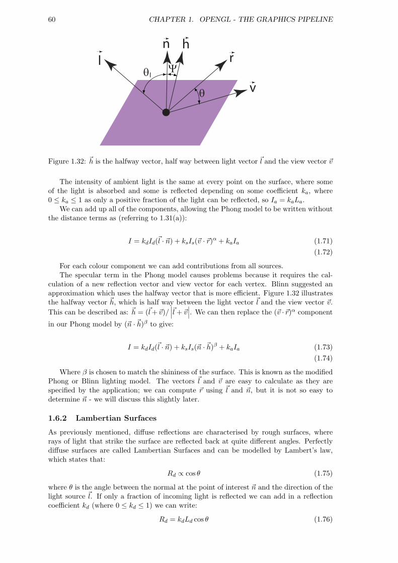
60 CHAPTER 1. OPENGL - THE GRAPHICS PIPELINE
n
θl
rl
v
h
θ
Ψ
Figure 1.32: ~h is the halfway vector, half way between light vector ~l and the view vector ~v
The intensity of ambient light is the same at every point on the surface, where someof the light is absorbed and some is reflected depending on some coefficient ka, where0 ≤ ka ≤ 1 as only a positive fraction of the light can be reflected, so Ia = kaLa.
We can add up all of the components, allowing the Phong model to be written withoutthe distance terms as (referring to 1.31(a)):
I = kdId(~l · ~n) + ksIs(~v · ~r)α + kaIa (1.71)(1.72)
For each colour component we can add contributions from all sources.The specular term in the Phong model causes problems because it requires the cal-
culation of a new reflection vector and view vector for each vertex. Blinn suggested anapproximation which uses the halfway vector that is more efficient. Figure 1.32 illustratesthe halfway vector ~h, which is half way between the light vector ~l and the view vector ~v.This can be described as: ~h = (~l +~v)/
∣∣∣~l + ~v∣∣∣. We can then replace the (~v ·~r)α component
in our Phong model by (~n · ~h)β to give:
I = kdId(~l · ~n) + ksIs(~n · ~h)β + kaIa (1.73)(1.74)
Where β is chosen to match the shininess of the surface. This is known as the modifiedPhong or Blinn lighting model. The vectors ~l and ~v are easy to calculate as they arespecified by the application; we can compute ~r using ~l and ~n, but it is not so easy todetermine ~n - we will discuss this slightly later.
1.6.2 Lambertian Surfaces
As previously mentioned, diffuse reflections are characterised by rough surfaces, whererays of light that strike the surface are reflected back at quite different angles. Perfectlydiffuse surfaces are called Lambertian Surfaces and can be modelled by Lambert’s law,which states that:
Rd ∝ cos θ (1.75)
where θ is the angle between the normal at the point of interest ~n and the direction of thelight source ~l. If only a fraction of incoming light is reflected we can add in a reflectioncoefficient kd (where 0 ≤ kd ≤ 1) we can write:
Rd = kdLd cos θ (1.76)

1.6. OPENGL SHADING 61
The amount of light is proportional to the vertical component of the incoming light. Ifwe used only the ambient and diffuse properties our materials would appear dull as weare missing the highlights on the surface. The highlights that we see on a reflectivesurface are usually different from the colour of the ambient and diffuse light, for examplea silver shiny metal ball viewed under white light will reflect a white highlight in thedirection of the viewer. This is the specular property of the surface and is associated witha smooth surface, rather than the rough surface associated with a diffuse model. Modellingrealistic specular surfaces is complex because the pattern by which light is scattered is notsymmetric and depends on the reflection angle. Phong proposed an approximate modelfor specular surfaces, which assumes that the surface is smooth for the specular reflection.The Phong model uses the equation:
Is = ksLscosαφ (1.77)
which gives the specular light that a viewer sees at a particular point on the surface,where the coefficient ks (where 0 ≤ ks ≤ 1) is the faction of incoming specular light thatis reflected, the exponent α is the shininess coefficient (where when α is increased thelight is concentrated on a narrower region centered on the angle of a perfect reflector, i.e.as α → ∞ (typically values of 200 to 500) we get a perfect mirror), and α is the anglebetween ~r a perfect reflector and ~v, the direction of the viewer.
1.6.3 The Normal Vector
With smooth surfaces the vector normal to the surface exists at every point and gives thelocal orientation of the surface. A surface normal, or just normal to a flat surface is a three-dimensional vector which is perpendicular to that surface (orthogonal). For a polygon, thesurface normal can be calculated as the vector cross product of two (non-parallel) vectoredges of the polygon. For a plane given by the equation ax+by+cz +d = 0; this equationcan be rewritten in terms of the normal to the plane as:
~n · (P − P0) = 0 (1.78)
where P is any point on the plane. If we have three non-colinear points P0, P1 and P2
(and therefore a plane) then the vectors P1 −P0 and P2 −P0 can be used to calculate thenormal as:
~n = (P2 − P0)× (P1 − P0) (1.79)
Figure 1.33 illustrates the calculation of the normal vector for a plane.In OpenGL a normal can be associated with a vertex through:
0 glNormal3f(Nx, Ny, Nz);glNormal3fv(pointerToNormal);
Normals are state variables that can be associated with all the vertices and can be used forthe lighting calculations at all of the vertices. Unfortunately, we are expected to calculatethese normals ourselves.
The OpenGL Red Book gives an example of the use of normals with the creation of aicosahedron.
0 void drawGLIcosahedron() // From the red book{
GLfloat x,y,z, c = 3.14159f/180.0f;#define X .525731112119133606#define Z .850650808352039932
5static GLfloat vdata[12][3] = {
{−X, 0.0, Z}, {X, 0.0, Z}, {−X, 0.0, −Z}, {X, 0.0, −Z},{0.0, Z, X}, {0.0, Z, −X}, {0.0, −Z, X}, {0.0, −Z, −X},{Z, X, 0.0}, {−Z, X, 0.0}, {Z, −X, 0.0}, {−Z, −X, 0.0}
10 };static GLuint tindices [20][3] = {
{0,4,1}, {0,9,4}, {9,5,4}, {4,5,8}, {4,8,1},{8,10,1}, {8,3,10}, {5,3,8}, {5,2,3}, {2,7,3},

62 CHAPTER 1. OPENGL - THE GRAPHICS PIPELINE
P
n
u
v P
n
P2
P1
P0
(a) (b)
Figure 1.33: (a) Illustrates the calculation of the normal ~n from two vectors ~u and ~v, using~n = ~u×~v and (b) illustrates the calculation of the normal using three non-colinear pointsas ~n = (P2 − P0)× (P1 − P0).
{7,10,3}, {7,6,10}, {7,11,6}, {11,0,6}, {0,1,6},15 {6,1,10}, {9,0,11}, {9,11,2}, {9,2,5}, {7,2,11} };
int i ;glBegin(GL TRIANGLES);
for ( i = 0; i < 20; i++) {
20 GLfloat d1[3], d2 [3], norm[3];for (int j = 0; j < 3; j++) {
d1[j ] = vdata[tindices[ i ][0]][ j ] − vdata[tindices[ i ][1]][ j ];d2[j ] = vdata[tindices[ i ][1]][ j ] − vdata[tindices[ i ][2]][ j ];
}25 normcrossprod(d1, d2, norm);
glNormal3fv(norm);
glVertex3fv(&vdata[tindices[ i ][0]][0]);glVertex3fv(&vdata[tindices[ i ][1]][0]);
30 glVertex3fv(&vdata[tindices[ i ][2]][0]);}
glEnd();}
35 void normalize(float v[3]) {GLfloat d = sqrt(v[0]∗v[0]+v[1]∗v[1]+v[2]∗v [2]);if (d == 0.0) {
return;}
40 v[0] /= d; v[1] /= d; v[2] /= d;}
void normcrossprod(float v1[3], float v2 [3], float out [3]){
45 GLint i, j ;GLfloat length;out[0] = v1[1]∗v2[2] − v1[2]∗v2[1];out[1] = v1[2]∗v2[0] − v1[0]∗v2[2];out[2] = v1[0]∗v2[1] − v1[1]∗v2[0];
50 normalize(out);}
Example1k illustrates this example... see 1.34. As stated, Gouraud proposed the useof the normals around a mesh vertex. Gouraud shading finds the average normal at eachvertex and applies the modified Phong model at each vertex. It then Interpolates vertexshades across each polygon. Phong shading finds the vertex normals; interpolates thevertex normals across the edges; interpolates edge normals across the polygon and thenapplies the modified Phong model at each fragment.
If the polygon mesh approximates a surface with a high curvature then Phong shadingtends to look much smoother, while Gouraud shading tends to show up edges. Phongshading requires much more computational effort than Gouraud shading - It was not untilrecently that Phong shading was available in real-time, by using fragment shaders. Bothof these shading schemes need data structures to represent the mesh, by which shadingcalculations can be performed.

1.6. OPENGL SHADING 63
Figure 1.34: These images give examples of the calculation of normals for an icosahedron.
n
n1 n3
n2 n4
Figure 1.35: Smooth Shading - Normals at vertices
1.6.4 Shading
One of the problems with the calculation of these normals is that it is computationallyintensive. OpenGL uses the efficiencies possible for rendering flat surfaces, by decomposingcurved surfaces into many small flat polygons. We will look at the different shading modelsused in OpenGL.
Flat Shading
The three vectors ~l (light), ~v (viewer) and ~n (normal) vectors which describe how an objectshould appear. If the light source and viewer are distant (or simply far away relative to thesize of a polygon) and if we assume a flat polygon, then ~n is constant over the polygon, thenthe shading calculation need only be carried out once for each polygon and each polygonis given the same shade. With OpenGL we can set flat (constant) shading through a call:
0 glShadeModel(GL FLAT);
OpenGL will use the normal associated with the first vertex of a polygon for all verticesof that polygon if flat shading is enabled. This shading method is not very attractive ashumans are very good at noticing shading intensity changes at linear boundaries (e.g. asquare of different shaded paint on a wall painted with a similar shade of paint).
Smooth Shading
OpenGL also provides us with a smooth shading model, which can be enabled using:
0 glShadeModel(GL SMOOTH);

64 CHAPTER 1. OPENGL - THE GRAPHICS PIPELINE
Figure 1.35 illustrates the normals at four connected polygons. Mathematically speak-ing, the calculation of a normal at a vertex should cause concern, as it is discontinuousat this point. However, Gouraud showed that by defining a normal at a vertex thatsmoother shading could be achieved over an object by using interpolation. In this figurewe can calculate the normal ~n at this vertex by using:
~n =~n1 + ~n2 + ~n3 + ~n4
|~n1 + ~n2 + ~n3 + ~n4|(1.80)
This should not be very difficult from an OpenGL as all we have to do is specify thenormals at the vertices and let OpenGL do the interpolation; however, it is not thatsimple as we do not tend to store the polygons in an order that allows us to average thesepolygons together. We would have to set up a data structure to store our models thatputs the vertices first, i.e. stores four polygons for each vertex.
The default setup is to shade only front faces of objects, which is fine for convex objects;however, if we need to allow back faces to be seen, then we can set two sided shading tobe enabled, using the glMaterialf() function with the properties GL FRONT, GL BACK andGL FRONT AND BACK.
1.6.5 Lighting
As previously discussed, OpenGL supports four types of light sources, ambient, point,spotlight and distant. We can set up the position of a light using a call to:
0 glLightfv(GLenum source, GLenum parameter, GLfloat ∗pointer to array);
Shading calculations are enabled using a call to glEnable(GL LIGHTING) we still haveto enable each light source individually using glEnable(GL LIGHTi), where i = 0, 1, . . . n,where n is defined by your graphic card.
Allows us to create a light, where we first have to set up the required parameters, suchas:
0 GLfloat light pos [] = {−1.0f, 1.0f , 2.0f , 1.0f};GLfloat light Ka[] = {0.0f, 0.0f , 0.0f , 1.0f};GLfloat light Kd[] = {1.0f, 1.0f , 1.0f , 1.0f};GLfloat light Ks [] = {1.0f, 1.0f , 1.0f , 1.0f};
5 glLightfv(GL LIGHT0, GL POSITION, light pos);glLightfv(GL LIGHT0, GL AMBIENT, light Ka);glLightfv(GL LIGHT0, GL DIFFUSE, light Kd);glLightfv(GL LIGHT0, GL SPECULAR, light Ks);
10 glEnable(GL LIGHTING);glEnable(GL LIGHT0);
Where the light position is specified using a homogeneous co-ordinate system. Thefourth parameter of Ka, Kd and Ks calls specify the alpha property of the ambient,diffuse and specular components of the light source. We then associate the arrays withthe GL POSITION, GL AMBIENT, GL DIFFUSE and GL SPECULAR properties of the light sourceGL LIGHT0. Finally, we have to enable the GL LIGHT0 and if necessary enable lighting onthe OpenGL machine. The light position is given in homogeneous co-ordinates, where the4th parameter is 1.0f if we are specifying a finite location, or 0.0f if we are specifying aparallel source with the given direction vector. The coefficients in the distance terms aregiven by default as a = 1.0, the constant terms; b = c = 0.0f , the linear and quadraticterms. If we wish to change these values we can do this by:
0 glLightfv(GL LIGHT0, GL CONSTANT ATTENUATION, 0.50f);//Also have GL LINEAR ATTENUATION and GL QUADRATIC ATTENUATION

1.6. OPENGL SHADING 65
Figure 1.36: The Nate Robins Tutorial Example on Light Positioning
Figure 1.36 demonstrates the positioning of light in a scene. If we wished to have ambientlight we can use:
0 GLfloat ambient light [] = {0.1, 0.1, 0.1, 1.0};glLightModelfv(GL LIGHT MODEL AMBIENT, ambient light);
Example1j illustrates the use of point lights and ambient lights.We can convert a point source to a spotlight by setting up a spotlight direction property
GL SPOT DIRECTION, the exponent GL SPOT EXPONENT and the angle GL SPOT CUTOFF. Weuse the same glLightfv() method to set these properties up. Depending on the graphiccard we are limited in the number of light sources that may be present.
1.6.6 OpenGL code for Shading
The Nate Robins’ Tutorial gives an excellent example of the use of OpenGL code forspecifying light and material properties. See Figures 1.36 and 1.38.

66 CHAPTER 1. OPENGL - THE GRAPHICS PIPELINE
Figure 1.37: This figure illustrates the use of a point light and an ambient light. Theimage on the left shows the three spheres lit by the ambient light only and the image onthe right shows the spheres having rotated into the beam of the light and view of observer.
Figure 1.38: The Nate Robins Tutorial on Light and Materials in OpenGL (lightmate-rial.exe). You can right click the various parameters to change their values.

Chapter 2
Scene Graph Theory
2.1 Introduction
In a previous section of this module you have experienced the use of the Java3D APIand its associated scene-graph. In this section of the module we are going to examinescene graphs in more detail, in particular examining how we can build our own type ofscene graph, which suits our particular application. To do this we are going to have tounderstand how we can organise a scene into a tree structure, how we can traverse thistree and how we can use this tree to represent complex concepts such as describing therelationship between objects, lights and cameras.
So, what is a scene graph? Well, the scene graph we are concerned with is a collectionof nodes ordered into a graph or tree structure. Each node can have many children, butusually each child has only one parent. This is quite similar to the object-oriented treesthat you would have seen in EE553 - object-oriented programming - in fact, more closelyassociated with the inheritance trees found in Java. Within a scene graph, operationsthat are applied to an object are propagated to the child nodes. As such, scene graphs arevery useful for representing complex geometries, and operations such as transformation,selections etc. which can be applied to all components of the object.
For example, a car could have a body and four rotating wheels; the wheels are posi-tioned and rotate relative to the body of the car, so a translation applied to the car bodyshould have an equivalent translation effect on the four wheels. This allows us to treat thecar with wheels as a single object and reduces the complexity of our application. Further-more, as memory and performance are always concerns in 3-D graphics, a well structuredscene graph would allow us to create reference nodes to geometries. In the example of thecar, this would allow us to define the geometry of the car’s wheel only once and use threereferences to position three ‘copies’ of the wheel that have been rotate and translated tothe correct location. To do this we would use a directed acyclic graph (DAG), which is ageneralisation of a tree in which certain subtrees can be shared by different parts of thetree, greatly reducing the memory footprint of our scene when there is repetition of sceneobjects - a Java3D Scene Graph is a DAG.
It should be clear at this stage that the concept of a scene graph is a clear candidatefor an object-oriented approach. This is certainly the case, but a word of warning atthis stage - OpenGL has a state-machine structure, which does not sit very well with theobject-oriented structure that we are going to impose on our scenes. It is worth mentioningthat scene graphs have found use in non-3D applications where there is a requirement tomanage the contents of spatially oriented data; in particular, MPEG4 uses a scene graphprogramming model for multimedia scene composition.
67

68 CHAPTER 2. SCENE GRAPH THEORY
2.2 A Simple Scene Graph Implementation
There are many scene graphs available including the Java3D API, Virtual Reality ModelingLanguage (VRML) and indeed Open Scene Graph and they have specific tasks in mind.For this module we are going to create our own simple scene graph to demonstrate howthey work.
The simplest type of scene graph would use an array data structure to store the objectsof the scene graph. We would iterate over the array to display the object in the scene,simply traversing from the first element in the array to the Nth element whenever we needto update the display. For small scenes this would be fine, but when we have a large scene,which may contain thousands of scene objects, this linear display will become noticeablyslow. Larger scene graphs tend to use tree structures to contain the scene objects as thehierarchical relationship it provides allows significant performance efficiencies. For the carexample, if we decided not to draw the car, then we could skip the scene objects whichcontained the four wheels etc.
A scene graph is an organised hierarchy of nodes; an n-ary tree, where a node cancontain any number of children, which can inherit the transformations and states of theparent objects. To organise a scene into a tree we generally use nodes such as groupnodes and leaf nodes. Group nodes usually have many nodes attached and can oftenhave a transformation or switching function. Leaf nodes usually contain renderable sceneobjects, such as graphical geometry objects, or non-graphical scene objects such as images,lights, cameras, materials and even sounds.
The reason that we use an object-oriented programming approach is so that we canbuild a future-proofed extensible core engine for our visualisation systems. From EE553object-oriented programming, you are probably aware that the features that are impor-tant to our scene graph design are inheritance and polymorphism. Inheritance allows usto define scene objects from other scene objects, and to extend or replace some of thefunctionality of the base class. Polymorphism allows us to use the virtual keyword tocall methods of derived classes using pointers that have a static type of the base class.The object-oriented structure is also very useful in managing the data in our scene, inparticular avoiding memory leaks as our visualisation system must be capable of runningfor a long period of time.
As stated, the n-ary tree is used to contain scene objects and the idea of an array wasdiscussed. A more appropriate method would be to use the ANSI/ISO C++ StandardTemplate Library (STL). STL is a collection of container classes, with associated iteratormechanisms and algorithms. It provides classes for stacks, queues, linked-lists, deques(double ended queues), maps, sets and vector storage containers. All of these containersare useful in building our tree structures. We have chosen the vector class container forour implementation as it provides a simple to use random access container; in effect it isan advanced random access dynamic array. Iterators are used to move through the datastructure and access its information.
Example Scene Graph Object Class
Here is our first design of our generic Scene Object base class:
0 // SceneObject.h− This is the base object of all objects in// the scene graph.//////////////////////////////////////////////////////////////////////
#if !defined SCENEOBJECT H5 #define SCENEOBJECT H
#include<vector> // Use the STL Vector as our container
enum RTTI OBJECT TYPE

2.2. A SIMPLE SCENE GRAPH IMPLEMENTATION 69
10 {RTTI CAMERA, //does not exist yetRTTI LIGHT, //does not exist yetRTTI DUMMY,
};15
class SceneObject{
protected:20 SceneObject∗ parentObject;
std :: vector<SceneObject∗> childrenObjects;
public:SceneObject();
25 virtual ˜SceneObject();
// assessors/mutatorsvoid setParent(SceneObject∗ parent) { parentObject = parent; }void addChild(SceneObject∗ child);
30 std :: vector<SceneObject∗>∗ getChildrenObjects() { return &childrenObjects; }virtual RTTI OBJECT TYPE getType() const = 0;
// Force every child to have a render and update methodsvirtual void render(float timeElapsed) = 0;
35 virtual void update(float timeElapsed) = 0;};
#endif // SCENEOBJECT H
And its associated C++ file:
0 // SceneObject.cpp: implementation of the SceneObject class.////////////////////////////////////////////////////////////////////////
#include <iostream>5 #include ”SceneObject.h”
SceneObject::SceneObject() {}
SceneObject::˜SceneObject() {}10
void SceneObject::addChild(SceneObject ∗child){
if (! child) { std :: cerr << ”Attempt to add invalid child to scene graph.”; }
15 child−>setParent(this);childrenObjects.push back(child);
}
Before this class begins we can see the RTTI OBJECT TYPE enumeration. As discussed,we will use polymorphism extensively. So a pointer with a static type of SceneObjectwill sometimes need to know what kind of object this pointer is actually pointing to (i.e.the dynamic type). This enumeration allows us to “name”’ the current object type. Thelist that is here is an example list for a camera, a light and a dummy object. We willextend this list later. In effect, an enum call simply numbers the list of constants. If youhave studied Java you will be aware of a Class class, which performs the same operation.This implementation of run-time type information (RTTI) allows a constant to defineexactly what kind of object we are dealing with at run-time. We can then simply use the

70 CHAPTER 2. SCENE GRAPH THEORY
getType() method to extract the dynamic type of the object that is currently pointed to.
Example Dummy Object Class
We can create various different scene objects. For now, we will just us a Dummy objectthat does not involve any 3-D graphics; rather, it will just output the name of the objectto the standard output stream (std::cout).
0 // DummyObject.h: interface for the DummyObject class.////////////////////////////////////////////////////////////////////////
#if !defined DUMMYOBJECT H5 #define DUMMYOBJECT H
#include <iostream>#include <string>#include ”SceneObject.h”
10
class DummyObject : public SceneObject{protected:
std :: string name;15
public:DummyObject(std::string dummyName);virtual ˜DummyObject();
20 virtual RTTI OBJECT TYPE getType() const { return RTTI DUMMY; }
virtual void render(float timeElapsed) {}virtual void update(float timeElapsed)
{25 std :: cout << ”Updating [” << name << ”] scene object ” << std::endl;
}};
#endif // DUMMYOBJECT H
And its associated C++ file:
0 // DummyObject.cpp: implementation of the DummyObject class.////////////////////////////////////////////////////////////////////////
#include <string>5 #include ”DummyObject.h”
DummyObject::DummyObject(std::string dummyName){
name = dummyName;10 }
DummyObject::˜DummyObject() {}
2.2.1 Traversing the Scene Graph
Once we have our scene graph structure of choice in place it is important that we are ableto interact with its information. The most basic operation is traversing the scene graph;that is, moving from one scene graph item to the next scene graph item. In the case of a
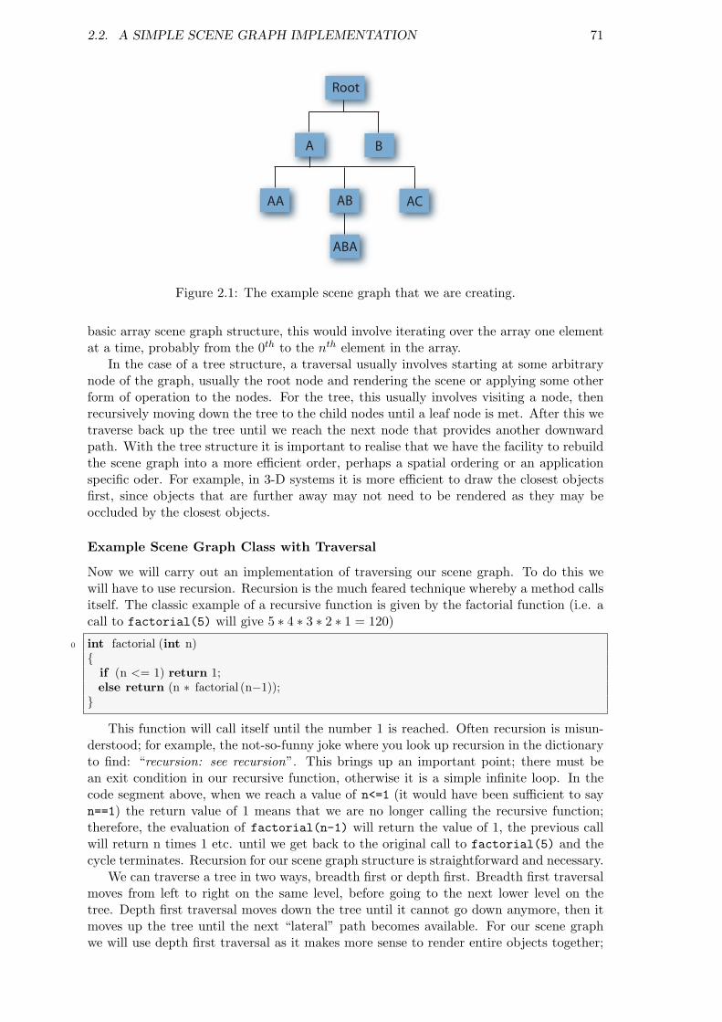
2.2. A SIMPLE SCENE GRAPH IMPLEMENTATION 71
Root
A B
AA AB AC
ABA
Figure 2.1: The example scene graph that we are creating.
basic array scene graph structure, this would involve iterating over the array one elementat a time, probably from the 0th to the nth element in the array.
In the case of a tree structure, a traversal usually involves starting at some arbitrarynode of the graph, usually the root node and rendering the scene or applying some otherform of operation to the nodes. For the tree, this usually involves visiting a node, thenrecursively moving down the tree to the child nodes until a leaf node is met. After this wetraverse back up the tree until we reach the next node that provides another downwardpath. With the tree structure it is important to realise that we have the facility to rebuildthe scene graph into a more efficient order, perhaps a spatial ordering or an applicationspecific oder. For example, in 3-D systems it is more efficient to draw the closest objectsfirst, since objects that are further away may not need to be rendered as they may beoccluded by the closest objects.
Example Scene Graph Class with Traversal
Now we will carry out an implementation of traversing our scene graph. To do this wewill have to use recursion. Recursion is the much feared technique whereby a method callsitself. The classic example of a recursive function is given by the factorial function (i.e. acall to factorial(5) will give 5 ∗ 4 ∗ 3 ∗ 2 ∗ 1 = 120)
0 int factorial (int n){
if (n <= 1) return 1;else return (n ∗ factorial (n−1));
}
This function will call itself until the number 1 is reached. Often recursion is misun-derstood; for example, the not-so-funny joke where you look up recursion in the dictionaryto find: “recursion: see recursion”. This brings up an important point; there must bean exit condition in our recursive function, otherwise it is a simple infinite loop. In thecode segment above, when we reach a value of n<=1 (it would have been sufficient to sayn==1) the return value of 1 means that we are no longer calling the recursive function;therefore, the evaluation of factorial(n-1) will return the value of 1, the previous callwill return n times 1 etc. until we get back to the original call to factorial(5) and thecycle terminates. Recursion for our scene graph structure is straightforward and necessary.
We can traverse a tree in two ways, breadth first or depth first. Breadth first traversalmoves from left to right on the same level, before going to the next lower level on thetree. Depth first traversal moves down the tree until it cannot go down anymore, then itmoves up the tree until the next “lateral” path becomes available. For our scene graphwe will use depth first traversal as it makes more sense to render entire objects together;

72 CHAPTER 2. SCENE GRAPH THEORY
for example, in the case of the car discussed earlier, to render the body and then the fourwheels, rather than move directly to the next object in the scene.
Here is a very basic Scene Graph Class:
0 // SceneGraph.h: interface for the SceneGraph class.////////////////////////////////////////////////////////////////////////
#if !defined SCENEGRAPH H5 #define SCENEGRAPH H
class SceneObject; //avoid a circular definition
class SceneGraph10 {
public:
SceneGraph();virtual ˜SceneGraph();
15
void updateScene(SceneObject∗ sceneObject, float timeElapsed);};
#endif // SCENEGRAPH H
And its associated C++ file which includes the code for traversal:
0 // SceneGraph.cpp: implementation of the SceneGraph class.////////////////////////////////////////////////////////////////////////
#include ”SceneGraph.h”5 #include ”SceneObject.h”
#include <vector>#include <iostream>
SceneGraph::SceneGraph() {}10
SceneGraph::˜SceneGraph() {}
void SceneGraph::updateScene(SceneObject∗ sceneObject, float timeElapsed){
15 if (! sceneObject){
std :: cerr << ”Attempt update of object not on the scene graph.”;return;
}20 else
{sceneObject−>update(timeElapsed);// and call all the childrenstd :: vector<SceneObject∗>::iterator it =
25 sceneObject−>getChildrenObjects()−>begin();for (; it !=sceneObject−>getChildrenObjects()−>end(); ++it){
updateScene(∗it, timeElapsed);}
30 }}
In this code segment we have the SceneGraph::updateScene() method which takes asceneObject and recursively calls the update() method on each of the object’s children

2.2. A SIMPLE SCENE GRAPH IMPLEMENTATION 73
using a depth first tree traversal. We use the STL vector iterator, so the vector of childobjects has a starting point, provided by begin() and an ending point, provided by end();we simply move the iterator over this range by using the ++it call in the for loop.
Here is an example of the construction of an example scene graph using the classesabove. In this example we pass a root node pointer to the SceneGraph::updateScene()method, so that all scene objects are updated.
0 /∗∗∗∗∗∗∗∗∗∗∗∗∗∗∗∗∗∗∗∗∗∗∗∗∗∗∗∗∗∗∗∗∗∗∗∗∗∗∗∗∗∗∗ EE563 Example Project 4 − Scene Graph Example∗ by: Derek Molloy∗∗∗∗∗∗∗∗∗∗∗∗∗∗∗∗∗∗∗∗∗∗∗∗∗∗∗∗∗∗∗∗∗∗∗∗∗∗∗∗∗∗/
5 #include <windows.h> // Header File For Windows#include <gl\gl.h> // Header File For The OpenGL32 Library#include <gl\glu.h> // Header File For The GLu32 Library#include ”vec3.h”#include ”Matrix.h”
10 #include ”vec4.h”#include ”Quat.h”#include ”SceneGraph.h”#include ”DummyObject.h”#include <iostream>
15 using namespace std;
int main(){
SceneGraph ∗sg = new SceneGraph;20
std :: cout << ”Creating Scene Objects \n”;
DummyObject ∗root = new DummyObject(”Dummy Root”);DummyObject ∗dummya = new DummyObject(”Dummy A”);
25 DummyObject ∗dummyb = new DummyObject(”Dummy B”);root−>addChild(dummya);root−>addChild(dummyb);DummyObject ∗dummyaa = new DummyObject(”Dummy AA”);DummyObject ∗dummyab = new DummyObject(”Dummy AB”);
30 DummyObject ∗dummyac = new DummyObject(”Dummy AC”);DummyObject ∗dummyaba = new DummyObject(”Dummy ABA”);dummya−>addChild(dummyaa);dummya−>addChild(dummyab);dummya−>addChild(dummyac);
35 dummyab−>addChild(dummyaba);sg−>updateScene(root, 0.0f);
std :: cout << ”Scene Updated \n”;
40 system(”pause”);return 0;
}
The output of this application is:
Creating Scene ObjectsUpdating Dummy Root scene objectUpdating Dummy A scene objectUpdating Dummy AA scene objectUpdating Dummy AB scene objectUpdating Dummy ABA scene objectUpdating Dummy AC scene object

74 CHAPTER 2. SCENE GRAPH THEORY
Root
A B
AA AB AC
ABA
Figure 2.2: The depth first traversal that has taken place on this scene graph.
Updating Dummy B scene objectScene Updated
Press any key to continue . . .
2.2.2 Putting it Together: The Scene Graph with OpenGL
Now, we will take this scene graph structure and apply it to the 3-D world. To do this wewill need to add more concepts to our scene graph. The previous code example provides atemplate for adding any type of scene graph structure. We will begin with a Primitive type,which will allow us to describe primitives such as spheres, cubes etc. The implementationfor this discussion is Example 5.
0 #if !defined PRIMITIVE H#define PRIMITIVE H
#include ”SceneObject.h”
5 enum PRIMITIVE TYPE{
SPHERE,CUBE
};10
class Primitive : public SceneObject{private:
PRIMITIVE TYPE type;15 float size ;
float divisions ;
public:Primitive(PRIMITIVE TYPE, float, float);
20 virtual ˜Primitive();
virtual RTTI OBJECT TYPE getType() const { return RTTI PRIMITIVE; }
// Force every child to have a render and update methods25 virtual void render(float timeElapsed);
virtual void update(float timeElapsed);

2.2. A SIMPLE SCENE GRAPH IMPLEMENTATION 75
protected:virtual void drawSphere();
30
};
#endif // PRIMITIVE H
The Primitive extends the SceneObject class and so can be added directly to the scenegraph and can even have child nodes below it - maybe this is not ideal? but, this is ourscene graph structure, so we can do what we want.
Now, we must also describe a Transformation. Once again, this has been designed asa child of SceneObject so that it can be added directly to the scene graph, and can havefurther children - this is very important in the case of a transform node, as it would bemeaningless as a leaf node. The Transform class really just encapsulates a single matrix;we could provide much more advanced functionality here. The render method simplyapplies this matrix as described below:
0 #if !defined TRANSFORM H#define TRANSFORM H
#include ”SceneObject.h”#include ”Matrix.h”
5
class Transform : public SceneObject{private:
Matrix matrix;10
public:Transform(Matrix);virtual ˜Transform();
15 virtual RTTI OBJECT TYPE getType() const { return RTTI TRANSFORM; }
// Force every child to have a render and update methodsvirtual void render(float timeElapsed);virtual void update(float timeElapsed);
20 };
#endif // TRANSFORM H
And a segment of the C++ file:
0 void Transform::render(float timeElapsed){
glMultMatrixf(matrix.ptr());}
We can put this all together to give:0 /∗∗∗∗∗∗∗∗∗∗∗∗∗∗∗∗∗∗∗∗∗∗∗∗∗∗∗∗∗∗∗∗∗∗∗∗∗∗∗∗∗∗
∗ EE563 Example Project 5 − Scene Graph Example with Graphics∗ by: Derek Molloy∗∗∗∗∗∗∗∗∗∗∗∗∗∗∗∗∗∗∗∗∗∗∗∗∗∗∗∗∗∗∗∗∗∗∗∗∗∗∗∗∗∗/
5 #include <windows.h> // Header File For Windows#include <gl\gl.h> // Header File For The OpenGL32 Library#include <gl\glu.h> // Header File For The GLu32 Library#include ”vec3.h”#include ”Matrix.h”
10 #include ”vec4.h”#include ”Quat.h”#include ”SceneGraph.h”#include ”DummyObject.h”#include ”Primitive.h”
15 #include ”Transform.h”#include <iostream>using namespace std;

76 CHAPTER 2. SCENE GRAPH THEORY
20 HDC hDC=NULL; // Private GDI Device ContextHGLRC hRC=NULL; // Permanent Rendering ContextHWND hWnd=NULL; // Holds Our Window HandleHINSTANCE hInstance; // Holds The Instance Of The ApplicationGLfloat fov = 60.0f;
25 int downX = 0, downY = 0;float xOffset = 0.0f, yOffset = 0.0f;SceneGraph ∗sg;
// Function Declarations30
LRESULT CALLBACK WndProc (HWND hWnd, UINT message, WPARAM wParam,LPARAM lParam);
void enableOpenGL (HWND hWnd, HDC ∗hDC, HGLRC ∗hRC);int initGL(GLvoid);
35 int drawGLScene(float theta);void disableOpenGL (HWND hWnd, HDC hDC, HGLRC hRC);void defineGLSphere(GLfloat, GLfloat);void increaseFOV();void decreaseFOV();
40 void setFOV(GLfloat);
// WinMain − the starting point of our application
int WINAPI WinMain (HINSTANCE hInst, HINSTANCE hPrevInstance,45 LPSTR lpCmdLine, int iCmdShow)
{WNDCLASS wc;HGLRC hRC;hInstance = hInst;
50 MSG msg;BOOL bQuit = FALSE;float theta = 0.0f;
// register window class55 wc.style = CS OWNDC;
wc.lpfnWndProc = WndProc;wc.cbClsExtra = 0;wc.cbWndExtra = 0;wc.hInstance = hInstance;
60 wc.hIcon = LoadIcon (NULL, IDI APPLICATION);wc.hCursor = LoadCursor (NULL, IDC ARROW);wc.hbrBackground = (HBRUSH) GetStockObject (BLACK BRUSH);wc.lpszMenuName = NULL;wc.lpszClassName = ”EE553GLExample”;
65 RegisterClass (&wc);
// create main windowhWnd = CreateWindow (”EE553GLExample”, ”EE553 Example 5”,
WS CAPTION | WS POPUPWINDOW | WS VISIBLE,70 0, 0, 256, 256,
NULL, NULL, hInstance, NULL);
// enable OpenGL for the windowenableOpenGL (hWnd, &hDC, &hRC);
75 initGL();
// program main loopwhile (!bQuit){
80 // check for messagesif (PeekMessage (&msg, NULL, 0, 0, PM REMOVE)){
// handle or dispatch messagesif (msg.message == WM QUIT)
85 {bQuit = TRUE;
}else{
90 TranslateMessage (&msg);DispatchMessage (&msg);
}}else
95 {drawGLScene(theta);SwapBuffers (hDC);theta += 1.0f;Sleep (1);
100 }}// shutdown OpenGLdisableOpenGL (hWnd, hDC, hRC);// destroy the window explicitly
105 DestroyWindow (hWnd);return msg.wParam;
}
110 // Window Callback Process
LRESULT CALLBACK WndProc(HWND hWnd, UINT message, WPARAM wParam, LPARAM lParam){
switch (message)115 {
case WM RBUTTONDOWN: // if the right button is downsetFOV(60);xOffset=0.0f;yOffset=0.0f;
120 return 0;case WM LBUTTONDOWN:

2.2. A SIMPLE SCENE GRAPH IMPLEMENTATION 77
downX = (int)(short)LOWORD(lParam);downY = (int)(short)HIWORD(lParam);
case WM MOUSEMOVE: // if the mouse is moved125 if (wParam == MK LBUTTON) // and the left mouse button is down
{int xPos = (int)(short)LOWORD(lParam);int yPos = (int)(short)HIWORD(lParam);int diffx = xPos − downX;
130 int diffy = yPos − downY;xOffset+= ((float)diffx)/10;yOffset+= ((float)diffy)/10;
}return 0;
135 case WM CREATE:return 0;
case WM CLOSE:PostQuitMessage (0);return 0;
140 case WM DESTROY:return 0;
case WM KEYDOWN:switch (wParam){
145 case VK ESCAPE:PostQuitMessage(0);return 0;
case VK LEFT:xOffset−=0.1f;
150 return 0;case VK RIGHT:
xOffset+=0.1f;return 0;
case VK UP:155 yOffset−=0.1f;
return 0;case VK DOWN:
yOffset+=0.1f;return 0;
160 case VK F1: //F1 key pressedreturn 0;
}return 0;
case WM CHAR:165 switch(wParam)
{case ’a’ :
decreaseFOV();return 0;
170 case ’s ’ :increaseFOV();return 0;
}return 0;
175 default:return DefWindowProc (hWnd, message, wParam, lParam);
}}
180//Enable OpenGL
void enableOpenGL (HWND hWnd, HDC ∗hDC, HGLRC ∗hRC){
185 PIXELFORMATDESCRIPTOR pfd;int iFormat;// get the device context (DC)∗hDC = GetDC (hWnd);
190 // set the pixel format for the DCZeroMemory (&pfd, sizeof (pfd));pfd.nSize = sizeof (pfd);pfd.nVersion = 1;pfd.dwFlags = PFD DRAW TO WINDOW | PFD SUPPORT OPENGL | PFD DOUBLEBUFFER;
195 pfd.iPixelType = PFD TYPE RGBA;pfd.cColorBits = 24;pfd.cDepthBits = 16;pfd.iLayerType = PFD MAIN PLANE;iFormat = ChoosePixelFormat (∗hDC, &pfd);
200 SetPixelFormat (∗hDC, iFormat, &pfd);
// create and enable the render context (RC)∗hRC = wglCreateContext( ∗hDC );wglMakeCurrent( ∗hDC, ∗hRC );
205 }
// Setup our GL Sceneint initGL(GLvoid){
210 glShadeModel(GL SMOOTH); // Enable Smooth ShadingglClearColor(1.0f , 1.0f , 1.0f , 1.0f );// White BackgroundglClearDepth(1.0f); // Depth Buffer SetupglEnable(GL DEPTH TEST); // Enables Depth TestingglDepthFunc(GL LEQUAL); // The Type Of Depth Testing To Do
215 glHint(GL PERSPECTIVE CORRECTION HINT, GL NICEST);// Really Nice Perspective Calculations
sg = new SceneGraph;DummyObject ∗root = new DummyObject(”Root”);
220 sg−>bindRoot(root);
DummyObject ∗dummya = new DummyObject(”Dummy A”);DummyObject ∗dummyb = new DummyObject(”Dummy B”);root−>addChild(dummya);

78 CHAPTER 2. SCENE GRAPH THEORY
225 root−>addChild(dummyb);
Primitive ∗p = new Primitive(SPHERE, 1.0f, 36.0f);root−>addChild(p);
230 Matrix m1, m2;m1.makeTranslate(2.0f, 0.0f, 0.0f );Transform ∗t1 = new Transform(m1);root−>addChild(t1);Primitive ∗p1 = new Primitive(SPHERE, 2.5f, 20.0f);
235 t1−>addChild(p1);
m2.makeTranslate(−2.0f, 0.0f, 0.0f );Transform ∗t2 = new Transform(m2);root−>addChild(t2);
240 Primitive ∗p2 = new Primitive(SPHERE, 2.5f, 10.0f);t2−>addChild(p2);
return TRUE; // Initialization Went OK}
245void increaseFOV() {
if (fov<180.0f) fov+=1.0;}
250 void decreaseFOV(){if (fov>0.0f) fov−=1.0;
}
void setFOV(GLfloat f){255 if (f>0.0f && f<180.0f) fov = f;
}
// Called to update the scene − give us the animationint drawGLScene(float theta) // Draw the scene;
260 { // theta is amount to rotateglClear (GL COLOR BUFFER BIT | GL DEPTH BUFFER BIT); // Clear ScreenglPolygonMode(GL FRONT AND BACK, GL LINE); // display all mesh lines of the sphere
glMatrixMode(GL PROJECTION);265 glLoadIdentity();
gluPerspective(fov, 1.0, 0.1, 100.0);
glMatrixMode(GL MODELVIEW);glLoadIdentity();
270 gluLookAt(0.0, 0.0, 10.0, 0.0, 0.0, 0.0, 0.0, 1.0, 0.0);glTranslatef (xOffset, yOffset, 0);
glColor3f(0.0 f , 1.0f , 0.0f ); // greensg−>renderScene(0.0f);
275return TRUE; // Keep Going
}
// Disable OpenGL280 void disableOpenGL (HWND hWnd, HDC hDC, HGLRC hRC)
{wglMakeCurrent (NULL, NULL);wglDeleteContext (hRC);ReleaseDC (hWnd, hDC);
285 }
Where, the most important part is:
0 sg = new SceneGraph;DummyObject ∗root = new DummyObject(”Root”);sg−>bindRoot(root);
DummyObject ∗dummya = new DummyObject(”Dummy A”);5 DummyObject ∗dummyb = new DummyObject(”Dummy B”);
root−>addChild(dummya);root−>addChild(dummyb);
Primitive ∗p = new Primitive(SPHERE, 1.0f, 36.0f);10 root−>addChild(p);
Matrix m1, m2;m1.makeTranslate(2.0f, 0.0f, 0.0f );Transform ∗t1 = new Transform(m1);
15 root−>addChild(t1);Primitive ∗p1 = new Primitive(SPHERE, 2.5f, 20.0f);t1−>addChild(p1);
m2.makeTranslate(−2.0f, 0.0f, 0.0f );20 Transform ∗t2 = new Transform(m2);
root−>addChild(t2);
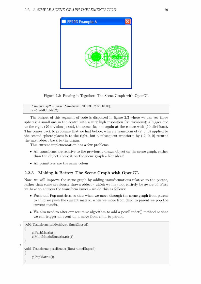
2.2. A SIMPLE SCENE GRAPH IMPLEMENTATION 79
Figure 2.3: Putting it Together: The Scene Graph with OpenGL
Primitive ∗p2 = new Primitive(SPHERE, 2.5f, 10.0f);t2−>addChild(p2);
The output of this segment of code is displayed in figure 2.3 where we can see threespheres; a small one in the centre with a very high resolution (36 divisions); a bigger oneto the right (20 divisions); and, the same size one again at the centre with (10 divisions).This comes back to problems that we had before, where a transform of (2, 0, 0) applied tothe second sphere places it to the right, but a subsequent transform by (-2, 0, 0) returnsthe next object back to the origin.
This current implementation has a few problems:
• All transforms are relative to the previously drawn object on the scene graph, ratherthan the object above it on the scene graph - Not ideal!
• All primitives are the same colour
2.2.3 Making it Better: The Scene Graph with OpenGL
Now, we will improve the scene graph by adding transformations relative to the parent,rather than some previously drawn object - which we may not entirely be aware of. Firstwe have to address the transform issues - we do this as follows:
• Push and Pop matrices, so that when we move through the scene graph from parentto child we push the current matrix; when we move from child to parent we pop thecurrent matrix.
• We also need to alter our recursive algorithm to add a postRender() method so thatwe can trigger an event on a move from child to parent.
0 void Transform::render(float timeElapsed){
glPushMatrix();glMultMatrixf(matrix.ptr());
}5
void Transform::postRender(float timeElapsed){
glPopMatrix();}

80 CHAPTER 2. SCENE GRAPH THEORY
And the recursive algorithm now becomes:
0 void SceneGraph::renderScene(SceneObject∗ sceneObject, float timeElapsed){
if (! sceneObject){
std :: cerr << ”Attempt update of object not on the scene graph.”;5 return;
}else{
sceneObject−>render(timeElapsed);10 // and call all the children
std :: vector<SceneObject∗>::iterator it =sceneObject−>getChildrenObjects()−>begin();
for (; it !=sceneObject−>getChildrenObjects()−>end(); ++it){
15 renderScene(∗it, timeElapsed);}
sceneObject−>postRender(timeElapsed); /∗∗∗∗ HERE ∗∗∗∗/}
20 }
To create a Material class, we can use:
0 // Material.h//////////////////////////////////////////////////////////////////////
#if !defined MATERIAL H#define MATERIAL H
5
#include ”SceneObject.h”#include ”Vec4.h”
class Material : public SceneObject10 {
private:Vec4 ambient;Vec4 diffuse ;Vec4 specular;
15 Vec4 emission;float shininess ;
public:Material();
20 virtual ˜Material();
virtual RTTI OBJECT TYPE getType() const { return RTTI MATERIAL; }
// Force every child to have a render and update methods25 virtual void render(float timeElapsed);
virtual void update(float timeElapsed);
virtual void setAmbient(Vec4 v) { ambient = v; }virtual void setDiffuse(Vec4 v) { diffuse = v; }
30 virtual void setSpecular(Vec4 v) { specular = v; }virtual void setEmission(Vec4 v) { emission = v; }virtual void setAmbient(float f) { shininess = f; }
};
35 #endif // MATERIAL H

2.2. A SIMPLE SCENE GRAPH IMPLEMENTATION 81
And the C++ file:
0 #include ”Material.h”#include ”gl/gl.h”
Material ::Material(){
5 ambient = Vec4(0.11f, 0.06f, 0.11f , 1.0f );diffuse = Vec4(0.43f, 0.47f , 0.54f , 1.0f );specular = Vec4(0.33f, 0.33f , 0.52f , 1.0f );emission = Vec4(0.00f, 0.00f , 0.00f , 0.0f );shininess = 10;
10 }
Material ::˜Material() {}
void Material::render(float timeElapsed)15 {
glMaterialfv(GL FRONT, GL AMBIENT, ambient.ptr());glMaterialfv(GL FRONT, GL DIFFUSE, diffuse.ptr());glMaterialfv(GL FRONT, GL SPECULAR, specular.ptr());glMaterialfv(GL FRONT, GL EMISSION, emission.ptr());
20 glMaterialfv(GL FRONT, GL SHININESS, &shininess);}
void Material::update(float timeElapsed){
25 std :: cout << ”Updating a Material ” << std::endl;}#endif // MATERIAL H
So, now we can create a scene graph as follows:
0 sg = new SceneGraph;DummyObject ∗root = new DummyObject(”Root”);sg−>bindRoot(root);
Light ∗l = new Light();5 root−>addChild(l);
Primitive ∗p = new Primitive(SPHERE, 1.0f, 36.0f);p−>getMaterial()−>setDiffuse(Vec4(0.18f, 0.81f, 0.31f, 1.0f )); //greenroot−>addChild(p);
10
Matrix m1, m2, m3;m1.makeTranslate(2.0f, 0.0f, 0.0f );Transform ∗t1 = new Transform(m1);root−>addChild(t1);
15 Primitive ∗p1 = new Primitive(SPHERE, 2.5f, 20.0f); //blue by defaultt1−>addChild(p1);
m2.makeTranslate(−2.0f, 0.0f, 0.0f );Transform ∗t2 = new Transform(m2);
20 root−>addChild(t2);Primitive ∗p2 = new Primitive(SPHERE, 2.5f, 10.0f);p2−>getMaterial()−>setDiffuse(Vec4(0.89f, 0.25f, 0.14f, 1.0f )); //redt2−>addChild(p2);
This is coded in Example 6, which gives the output as displayed by figure 2.4(a). Itcan then be altered easily, such as:
0 sg = new SceneGraph;

82 CHAPTER 2. SCENE GRAPH THEORY
Figure 2.4: Making it Better: The Scene Graph with OpenGL
...
m3.makeTranslate(0.0f, 1.25f, 0.0f );Transform ∗t3 = new Transform(m3);
5 p2−>addChild(t3);Primitive ∗p3 = new Primitive(SPHERE, 0.5f, 10.0f);p3−>getMaterial()−>setDiffuse(Vec4(0.89f, 0.25f, 0.14f, 1.0f )); //redt3−>addChild(p3);
Which gives the output as displayed by figure 2.4(b).
2.3 Constructive Solid Geometry (CSG)
Constructive Solid Geometry (CSG) is a technique whereby a complex model can becreated by using Boolean operations to combine a set of primitive shapes (spheres, cubes,cylinders etc.). It is generally used for rigid CAD type models of machinery and equipment,where it is possible that these complex models will be manufactured from such primitives.Figure 2.5 should illustrate the main concepts behind CSG - In this example we have theequation (A−B) ∪ (C ∩D), which is represented as a CSG tree in the same figure, withthe final output displayed in figure 2.6.
CSG does suffer from problems: The tree representation is quite straightforward, butthe computation time required to produce the final model is significant as 3-D Boolean

2.3. CONSTRUCTIVE SOLID GEOMETRY (CSG) 83
A B C D
A-B
C D
U
A B C D
-
U
U
Figure 2.5: CSG Example illustrating the shapes A, B, C, D; the result of A−B and ofC ∩D; and the associated CSG Tree.
Figure 2.6: CSG Example illustrating the result of (A− B) ∪ (C ∩D), in both solid andwireframe form (with hidden lines visible.)
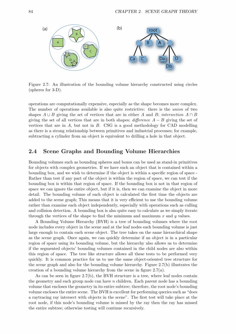
84 CHAPTER 2. SCENE GRAPH THEORY
A
B
C
D
(a)
Db
(b) root
AAB
C DADa
Db
Ca
Ca
Da
Figure 2.7: An illustration of the bounding volume hierarchy constructed using circles(spheres for 3-D).
operations are computationally expensive, especially as the shape becomes more complex.The number of operations available is also quite restrictive: there is the union of twoshapes A ∪ B giving the set of vertices that are in either A and B; intersection A ∩ Bgiving the set of all vertices that are in both shapes; difference A − B giving the set ofvertices that are in A, but not in B. CSG is a good methodology for CAD modellingas there is a strong relationship between primitives and industrial processes; for example,subtracting a cylinder from an object is equivalent to drilling a hole in that object.
2.4 Scene Graphs and Bounding Volume Hierarchies
Bounding volumes such as bounding spheres and boxes can be used as stand-in primitivesfor objects with complex geometries. If we have such an object that is contained within abounding box, and we wish to determine if the object is within a specific region of space -Rather than test if any part of the object is within the region of space, we can test if thebounding box is within that region of space. If the bounding box is not in that region ofspace we can ignore the entire object, but if it is, then we can examine the object in moredetail. The bounding volume of each object is calculated the first time the objects areadded to the scene graph; This means that it is very efficient to use the bounding volumerather than examine each object independently, especially with operations such as cullingand collision detection. A bounding box is also quite easy to calculate as we simply iteratethrough the vertices of the shape to find the minimum and maximum x and y values.
A Bounding Volume Hierarchy (BVH) is a tree of bounding volumes where the rootnode includes every object in the scene and at the leaf nodes each bounding volume is justlarge enough to contain each scene object. The tree takes on the same hierarchical shapeas the scene graph. Once again, we can quickly determine if an object is in a particularregion of space using its bounding volume, but the hierarchy also allows us to determineif the segmented objects’ bounding volumes contained in the child nodes are also withinthis region of space. The tree like structure allows all these tests to be performed veryquickly. It is common practice for us to use the same object-oriented tree structure forthe scene graph and also for the bounding volume hierarchy. Figure 2.7(b) illustrates thecreation of a bounding volume hierarchy from the scene in figure 2.7(a).
As can be seen in figure 2.7(b), the BVH structure is a tree, where leaf nodes containthe geometry and each group node can have n children. Each parent node has a boundingvolume that encloses the geometry in its entire subtree; therefore, the root node’s boundingvolume encloses the entire scene. The BVH is excellent for performing queries such as “doesa raytracing ray intersect with objects in the scene”. The first test will take place at theroot node, if this node’s bounding volume is missed by the ray then the ray has missedthe entire subtree; otherwise testing will continue recursively.

2.5. SPACE SUBDIVISION STRUCTURES 85
A B
A A
B
E
D
C C
A
B C
D E
Figure 2.8: A 2-D axis-aligned BSP Example, illustrating the segmentation of 2-D spaceA by a line that splits the space into two; the BSP tree is given on the right hand side
If the scene is dynamically changing then we can update the tree at runtime. If aparticular BV node has moved, we can very quickly check if it is still contained within itsparent BV. If it is then the BVH is valid, but if not, the node can be removed and theparent’s BVH must be recomputed. This can have implications further up the tree also.
2.5 Space Subdivision Structures
We have examined Scene Graph implementations that use trees to describe the high-levelrelationships between the various scene objects, and we have discussed CSG which usestrees to create the scene objects themselves. Now we will examine another use of the treestructure for describing the 3-D world itself in terms of its geometry, which will allow usto improve the real-time performance of our applications. The techniques to be discussedhere are used in a wide range of real-time applications, such as culling, collision detectionand ray tracing. Once again the relationships that we are going to represent with a treestructure are hierarchical, where the parent object in the hierarchy will enclose the childobject below it.
2.5.1 Binary Space Partitioning Trees
CSG Trees were used to describe the relationships between component parts of an objectand previously in our scene graph we used trees to represent the hierarchical relationshipbetween objects in a scene. Trees can also be used to capture the spatial relationshipbetween objects in a scene. This is particularly important when performing visibility testson the scene; if objects cannot be seen by the camera then from an efficiency perspectivethere is no point in rendering them to the scene.
Binary Space Partition Trees (or BSP trees for short) where introduced by Fuchs,Kedem, and Naylor around 1980 (?). The first ever computer game to use BSP trees wasDoom1, created by John Carmack and John Romero; since then all first person shootinggames have used this technique.
Binary Space Partitioning (BSP) is a technique for recursively subdividing a 3-D spaceinto two non-overlapping regions using a plane, referred to as a hyperplane2. Any pointin 3-D space lies within only one of these regions. BSP is a hierarchal approach wherethe space that is divided can be further subdivided using the same space partitioningapproach until some condition is met, resulting in a space-partitioning tree, which isparticularly useful when building techniques for dealing with hidden surface removal. Thebasic properties of BSPs are that objects on one side of a hyperplane cannot intercept anobject on the other side; and given a particular view point objects on the same side of thehyperplane are closer than objects on the other side.
The algorithm to build a BSP tree is fairly straightforward:1http://www.idsoftware.com2A hyperplane in n-dimensional space is an n − 1-dimensional object that can be used to divide the
n-dimensional space into two n-dimensional spaces - e.g. in 2-D a line is used

86 CHAPTER 2. SCENE GRAPH THEORY
0
0
0
1f 1b
1f 1b
0
0
0
1f 1b
1f 1b
2f
2b
2f 2b
0
0
1f 1b
1f 1b
2f
2b
2f 2b
3f3b
3f 3b
(a)
(c) (d)
(b)
Figure 2.9: This 2-D example illustrates the sample creation of a BSP Tree using linesto create the tree. Each line represents a partition plane (a) creates the partition planeand thus the root node, (b) through (d) illustrates the addition of further planes, with frepresenting the front side and b representing the back side.
• Select a partition plane - The choice of planes is application dependent, but oftenaxis aligned. In an ideal situation this will result in a balanced tree, but a poor choicewill result in a large number of splits and an increase in the number of polygons.There is usually a trade-off between a well-balanced tree and a large number of splits.
• Segment the current set of polygons using the chosen plane - If a polygon lies entirelyto one side or other of the plane then it is not modified and is added to the partitionset for the side that it is on. If the polygon spans the partition plane then it is splitinto two pieces, which are added to the set on the correct side of the plane.
• Repeat again using the new sets of polygons - The termination condition is a ap-plication specific, often based on a maximum number of nodes in a leaf node, ormaximum tree depth.
Figure 2.9 illustrates the core idea behind the creation of a non-axis aligned BSP treein the 2-D case. It takes a set of lines (polygons in the 3-D case) that is a part of a sceneand divides them into smaller sets, where each subset is a convex set of lines (i.e. each lineis in-front-of every other line in the same set. In this example we choose an arbitrary planein space and divide the lines, by putting the lines in the positive side of the plane in theleft subtree and the lines on the negatives side in the right sub tree. Where the partitionplanes intersect we divide the line (again, polygon in 3-D) according to the plane that theline defines. We can therefore split a line into two parts f(in front) and b(behind). Ascan be seen from this straightforward example, it will be difficult to balance the tree. Ifthere are too many polygons created in the tree then there will be a computational costin maintaining and rendering the tree, but if the tree is unbalanced it will be expensive totraverse.

2.5. SPACE SUBDIVISION STRUCTURES 87
Here is the C++ pseudo code on how you might code a BSP Tree3:
0 struct BSP tree{
plane partition ;list polygons;BSP tree ∗front , ∗back;
5 };
This struct stores the partitioning plane for the node, the list of polygons coincidentwith the partitioning plane and the pointers to its children. For this example, there willalways be at least one polygon in the coincident list and the child pointers will be initialisedto NULL.
0 void Build BSP Tree (BSP tree ∗tree, list polygons){
polygon ∗root = polygons.Get From List ();tree−>partition = root−>Get Plane();tree−>polygons.Add To List(root);
5 list front list , back list ;polygon ∗poly;
while ((poly = polygons.Get From List ()) != 0){
10 int result = tree−>partition.Classify Polygon (poly);switch (result){
case COINCIDENT:tree−>polygons.Add To List (poly);
15 break;case IN BACK OF:
back list .Add To List(poly);break;
case IN FRONT OF:20 front list .Add To List(poly);
break;case SPANNING:
polygon ∗ front piece , ∗back piece;Split Polygon (poly, tree−>partition, front piece , back piece);
25 back list .Add To List (back piece);front list .Add To List (front piece );break;
}}
30 if ( ! front list .Is Empty List()){
tree−>front = new BSP tree;Build BSP Tree (tree−>front, front list );
}35 if ( ! back list .Is Empty List())
{tree−>back = new BSP tree;Build BSP Tree (tree−>back, back list);
}40 }
This routine recursively constructs a BSP tree using the above algorithm. It takes thefirst polygon from the input list and uses it to partition the remainder of the set. Theroutine then calls itself recursively with each of the two partitions. This implementation
3Pseudo code modified from: http://www.opengl.org/resources/code/samples/bspfaq/

88 CHAPTER 2. SCENE GRAPH THEORY
(A) (B)
viewer
A A
B
C
DE
Figure 2.10: (a) Illustrates a viewer looking at 2-D objects in a scene; (b) Illustrates theactual objects that are seen by the viewer in this scene.
Figure 2.11: A simple test scene and the z-buffer representation
assumes that all of the input polygons are convex. Probably the most common applicationof BSP trees is hidden surface removal in 3-D. BSP trees provide an elegant, efficientmethod for sorting polygons via a depth first search . This fact can be exploited in a backto front “Painter’s Algorithm” approach to the visible surface problem, painting closeobjects first. The BSP Tree is particularly computationally efficient as the calculation canbe carried out in the pre-processing of the map and not at run-time.
2.6 Hidden Surface Removal
Visibility Testing is an important problem in 3-D Computer Graphics as it impacts on theefficiency of our algorithms: Very simply put, if an object is not visible then we should notdisplay it. So, figure 2.10(a) assumes we have a set of objects in our scene graph whichare in front of a viewer - should we display all these figures using OpenGL? Well no, ifwe look closely at the viewer and examine its field of view, we can see that only object Ais visible to the viewer. We wish to generate the image that the viewer would see and sojudging from 2.10(b) we would only have to render object a.
The simple solution would be to use a z-buffer (depth buffer), a buffer that stores thez-depth of each pixel currently at each point on the 2-D screen. If another object in thescene is to be rendered, the algorithm compares the depth value of the object’s renderingto the current screen z-buffer value at that pixel, and will choose the closer pixel. It updatethe z-buffer with the closest pixel (as demonstrated in 2.11).
The z-buffer approach was traditionally a very computationally expensive solution tothe depth test problem. It requires additional memory to store the z-buffer 2-D array andextra computational cost in performing the depth test at every pixel. A software algorithmwas developed to reduce this cost; the Painter’s Algorithm.

2.6. HIDDEN SURFACE REMOVAL 89
23
4
1
1 2
3
Figure 2.12: The simple Painters’s Algorithm shown on the LHS with the numbers rep-resenting the order in which the different regions are painted; 1 is painted first and 4 ispainted last. The RHS illustrates a situation where the Painter’s Algorithm fails as thereare no planes separating the objects in the scene.
2.6.1 The Painter’s Algorithm and BSP
The Painter’s Algorithm is a fairly simple algorithm for determining the visibility of poly-gons in 3-D computer graphics. The algorithm refers to a painter that paints the distantparts of the scene first and then paints this over with parts that are nearer (See figure2.12). The Painter’s Algorithm sorts all the polygons in the scene by their depth andthen paints them in the same order as the painter, from furthest to closest. This verysimple algorithm solves the visibility problem, but it has incurred the computational costof painting distant regions that will be painted over by closer regions. One condition fora successful painter’s algorithm is that there be a single plane which separates any twoobjects. This means that it might be necessary to split polygons in certain configurations.For example, the RHS of figure 2.12 illustrates a case that cannot be drawn correctly whenusing the painter’s algorithm.
One reason that BSP trees are appropriate for the Painter’s Algorithm is that splittingdifficult polygons can be an automated part of tree construction. To draw the contents ofthe tree you can perform a back to front tree traversal, which begins at the root node andclassifies the eye point with respect to its partition plane. We draw the subtree at the farchild from the eye, then the polygons in this node, followed by the near subtree. This isrepeated recursively for each subtree.
It is just as easy to traverse the BSP tree in front-to-back order as it is for the back-to-front order just discussed. We can use this to our advantage in a scan line renderer byusing a write mask which will prevent pixels from being written more than once. Thiswill produce significant speedups if a complex lighting model is evaluated for each pixel,because the painter’s algorithm will blindly evaluate the same pixel many times. The trickto making a scan line approach successful is to have an efficient method for masking pixels.One way to do this is to maintain a list of pixel spans which have not yet been written tofor each scan line. For each polygon scan converted, only pixels in the available spans arewritten, and the spans are updated accordingly. [add reference]
When building a BSP tree specifically for hidden surface removal, the partition planesare usually chosen from the input polygon set. However, any arbitrary plane can be usedprovided there are no intersecting or concave polygons, as in figure 2.12. Here is a simpleC++ pseudo code example of a back to front tree traversal:
0 void Draw BSP Tree(BSP tree ∗tree, point eye){
real result = tree−>partition.Classify Point(eye);if ( result > 0){

90 CHAPTER 2. SCENE GRAPH THEORY
5 Draw BSP Tree(tree−>back, eye);tree−>polygons.Draw Polygon List();Draw BSP Tree(tree−>front, eye);
}else if ( result < 0)
10 {Draw BSP Tree(tree−>front, eye);tree−>polygons.Draw Polygon List();Draw BSP Tree(tree−>back, eye);
}15 else // result is 0
{// the eye point is on the partition plane ...Draw BSP Tree(tree−>front, eye);Draw BSP Tree(tree−>back, eye);
20 }}
If the eye point is classified as being on the partition plane, the drawing order isunclear. This is not a problem if the Draw Polygon List routine is smart enough not todraw polygons that are not within the viewing frustum. The coincident polygon list doesnot need to be drawn in this case, because those polygons will not be visible to the user.It is possible to substantially improve the quality of this example by including the viewingdirection vector in the computation. You can determine that entire subtrees are behindthe viewer by comparing the view vector to the partition plane normal vector. This testcan also make a better decision about tree drawing when the eye point lies on the partitionplane. It is worth noting that this improvement resembles the method for tracing a raythrough a BSP tree, which is discussed in another section of the notes. Front to back treetraversal is accomplished in exactly the same manner, except that the recursive calls toDraw BSP Tree occur in reverse order.
As we have seen, the idea behind having a pre-calculated BSP tree is that it allowsus to get the correct depth order of polygons in the scene for any point in space. Figure2.13 illustrates the core operations on a BSP. In figure 2.13(a) a scene with 5 objectshas been partitioned using a simple polygon-aligned BSP Tree algorithm. In this scene,object E has been split by the partition lines into two separate objects, the larger parton the forward side of L3 and the larger part on the behind side of L3. 2.13(b) showsthe calculated BSP tree, where circular nodes represent the partition lines and squarenodes represent the leaf geometry nodes. In this example E∗ represents a partial objectE and f is the forward and b is the behind side of each partition line. Now, in 2.13(c)an observer enters the scene and we wish to calculate the nearest object. We can do thisby traversing the tree (rather than calculating the Euclidean distance to every object inthe scene). Starting at the root node, is the observer in front of, or behind L1? In thiscase the observer is behind L1, so in 2.13(d) we travel down the b side of the tree to L3,repeating this for L3 we find that the observer is again behind L3 and finally we find thatthe observer is in front of L5. At this point we find that the closest object to the observeris D. In 2.13(e) we see that we can then use this point to find the visibility order of all theobjects in the tree. Starting at D we traverse to the previous circular node, and then downthe tree, finding E∗ to be the next closest object. The path is traversed as illustrated in(e) until the visibility order is determined (in this case as, D, E∗, E∗, C, B, A, where Ais the most distant).
OpenGL achieves hidden surface removal through the use of a depth buffer and depthtesting. Depth buffering must be enabled with the command glEnable(GL DEPTH TEST).Before drawing a scene the depth buffer should be cleared with the command glClear(GLDEPTH BUFFER BIT). The command glCullFace(GLenum mode) indicates which polygonsshould be discarded (culled) before they are converted to screen coordinates. The param-eter mode is either GL FRONT, GL BACK, or GL FRONT AND BACK to indicate front-facing,

2.6. HIDDEN SURFACE REMOVAL 91
(a)
viewer
A
B
C
DE
L1
L2
L3
L4
L5
(b)L1
L2 L3
L4 L5A B
D EC E
f b
f bf
f f
b
b b
(c)
A
B
C
DE
L1
L2
L3
L4
L5
(d)L1
L2 L3
L4 L5A B
D EC E
f b
f bf
f f
b
b b
(e)L1
L2 L3
L4 L5A B
D EC E
1st
2nd3rd
4th
5th6th
* *
* *
* *
Figure 2.13: An illustration of the operations on a BSP Tree; (a) illustrates a simple scenewhich has been partitioned, (b) illustrates the creation of a BSP tree from (a), (c) shows aviewer entering the scene, (d) illustrates the algorithm for finding the closest object, and(d) illustrates a search to find the visibility order of all the objects.

92 CHAPTER 2. SCENE GRAPH THEORY
back-facing, or all polygons. To take effect, the state variable for culling, GL CULL FACEmust be enabled.
In OpenGL every polygon has a front and a back side. Each side can be drawnin the same mode or in different modes to allow cut-away views of solid objects. Thecommand glPolygonMode(GLenum face, GLenum mode) controls the drawing mode fora polygon’s front and back faces. The parameter face can be GL FRONT, GL BACK, orGL FRONT AND BACK. The mode can be GL POINT, GL LINE, or GL FILL to indicate whetherthe polygon should be drawn as points, outlined, or filled. By default, both the front andback faces are drawn filled:
0 glEnable(GL DEPTH TEST); // enable depth testing; required for z−buffer
glClear(GL DEPTH BUFFER BIT); // clears the depth bufferRenderScene(); // render the scene
Also, to draw the scene with back-face culling enabled (as it is more efficient), use:
0 glEnable(GL DEPTH TEST); // enable depth testing ; required for z−bufferglEnable(GL CULL FACE); // enable polygon face cullingglCullFace(GL BACK); // tell opengl to cull the back face
glClear(GL DEPTH BUFFER BIT); // clears the depth buffer5 RenderScene(); // render the scene

Chapter 3
Real-Time 3D Computer GraphicsTechniques
3.1 Introduction
This chapter will introduce various 3D Computer Graphics Techniques that we can use toaccelerate the systems that we build for real-time visualisation.
3.2 Texture Mapping in OpenGL
In 3D texture mapping a 2D image is attached to the surface of a polygon. This process canbe invaluable in creating realistic scenes within gaming and virtual reality environments.Texture mapping has evolved over the years to include features such as bump mapping,where the surface normals can be irregular to give the impression of texture changes onan object.
OpenGL uses raw RGB image data for texture mapping. The thing you have to dobefore OpenGL can use the raw texture data is upload it to the video memory. Once atexture is uploaded to the video memory it can be used throughout the time in which yourapplication is running.
Before a texture can be uploaded to the video memory there is some setup that musttake place so OpenGL knows what to do with the image data that is passed to it. First weneed a texture name. This is essentially a number that OpenGL uses to index all the differ-ent textures. To get a texture name, all we need do is call the function glGenTextures().
0 GLuint texture;glGenTextures( 1, &texture ); // only one texture id
where glGenTextures() has the form void glGenTextures( GLsizei n, GLuint *textures) where n is the number of texture ids to provide and the second parameter specifies thearray in which to store the ids (in my example here I only need one variable as I requireonly one texture).
Once the texture name is assigned we can then switch between our different texturesusing the glBindTexture() call - you can think of this in the same way that we switchcolours for painting.
0 glBindTexture( GL TEXTURE 2D, texture );
states that we wish to select our 2D texture that has the name texture. There are1D and 2D textures but we are concerned with 2D textures here. Remember that thisvalue is just an integer and we could probably have made the same call by something likeglBindTexture (GL TEXTURE 2D, 0).
93
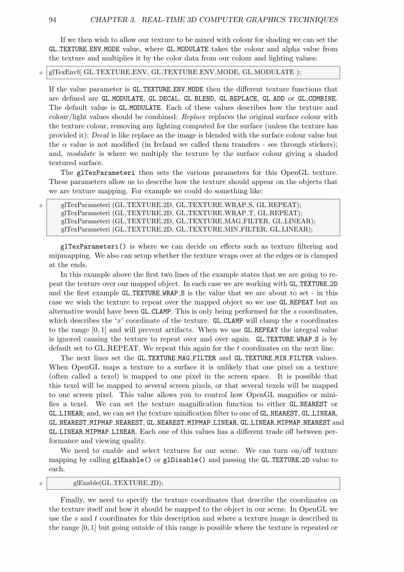
94 CHAPTER 3. REAL-TIME 3D COMPUTER GRAPHICS TECHNIQUES
If we then wish to allow our texture to be mixed with colour for shading we can set theGL TEXTURE ENV MODE value, where GL MODULATE takes the colour and alpha value fromthe texture and multiplies it by the color data from our colour and lighting values:
0 glTexEnvf( GL TEXTURE ENV, GL TEXTURE ENV MODE, GL MODULATE );
If the value parameter is GL TEXTURE ENV MODE then the different texture functions thatare defined are GL MODULATE, GL DECAL, GL BLEND, GL REPLACE, GL ADD or GL COMBINE.The default value is GL MODULATE. Each of these values describes how the texture andcolour/light values should be combined: Replace replaces the original surface colour withthe texture colour, removing any lighting computed for the surface (unless the texture hasprovided it); Decal is like replace as the image is blended with the surface colour value butthe α value is not modified (in Ireland we called them transfers - see through stickers);and, modulate is where we multiply the texture by the surface colour giving a shadedtextured surface.
The glTexParameteri then sets the various parameters for this OpenGL texture.These parameters allow us to describe how the texture should appear on the objects thatwe are texture mapping. For example we could do something like:
0 glTexParameteri (GL TEXTURE 2D, GL TEXTURE WRAP S, GL REPEAT);glTexParameteri (GL TEXTURE 2D, GL TEXTURE WRAP T, GL REPEAT);glTexParameteri (GL TEXTURE 2D, GL TEXTURE MAG FILTER, GL LINEAR);glTexParameteri (GL TEXTURE 2D, GL TEXTURE MIN FILTER, GL LINEAR);
glTexParameteri() is where we can decide on effects such as texture filtering andmipmapping. We also can setup whether the texture wraps over at the edges or is clampedat the ends.
In this example above the first two lines of the example states that we are going to re-peat the texture over our mapped object. In each case we are working with GL TEXTURE 2Dand the first example GL TEXTURE WRAP S is the value that we are about to set - in thiscase we wish the texture to repeat over the mapped object so we use GL REPEAT but analternative would have been GL CLAMP. This is only being performed for the s coordinates,which describes the ‘x’ coordinate of the texture. GL CLAMP will clamp the s coordinatesto the range [0, 1] and will prevent artifacts. When we use GL REPEAT the integral valueis ignored causing the texture to repeat over and over again. GL TEXTURE WRAP S is bydefault set to GL REPEAT. We repeat this again for the t coordinates on the next line.
The next lines set the GL TEXTURE MAG FILTER and GL TEXTURE MIN FILTER values.When OpenGL maps a texture to a surface it is unlikely that one pixel on a texture(often called a texel) is mapped to one pixel in the screen space. It is possible thatthis texel will be mapped to several screen pixels, or that several texels will be mappedto one screen pixel. This value allows you to control how OpenGL magnifies or mini-fies a texel. We can set the texture magnification function to either GL NEAREST orGL LINEAR; and, we can set the texture minification filter to one of GL NEAREST, GL LINEAR,GL NEAREST MIPMAP NEAREST, GL NEAREST MIPMAP LINEAR, GL LINEAR MIPMAP NEAREST andGL LINEAR MIPMAP LINEAR. Each one of this values has a different trade off between per-formance and viewing quality.
We need to enable and select textures for our scene. We can turn on/off texturemapping by calling glEnable() or glDisable() and passing the GL TEXTURE 2D value toeach.
0 glEnable(GL TEXTURE 2D);
Finally, we need to specify the texture coordinates that describe the coordinates onthe texture itself and how it should be mapped to the object in our scene. In OpenGL weuse the s and t coordinates for this description and where a texture image is described inthe range [0, 1] but going outside of this range is possible where the texture is repeated or

3.2. TEXTURE MAPPING IN OPENGL 95
Figure 3.1: The Nate Robins’ Tutorial on Texturing in OpenGL (texture.exe). You canright click the various parameters to change their values.
clamped. For a repeated texture the values [1, 2] will describe the exact same image. Sofor example:
0 glBegin( GL QUADS );glTexCoord2d(0.0f,0.0f); glVertex2d(0.0f ,0.0 f );glTexCoord2d(1.0f,0.0f); glVertex2d(1.0f ,0.0 f );glTexCoord2d(1.0f,1.0f); glVertex2d(1.0f ,1.0 f );glTexCoord2d(0.0f,1.0f); glVertex2d(0.0f ,1.0 f );
5 glEnd();
Will map the entire texture image to a single polygon.There is a good tutorial on texture mapping in the Nate Robins’ tutors set. Figure
3.1 illustrates this tutorial in action.In the case of the polygon above we specified the texture coordinates for each vertex.
This is not too difficult as there are only four texture coordinates for the polygon andthey align with those of a standard image. It can become more difficult when the texturecoordinates are on more complex objects. On a sphere with 36 subdivisions in longitudeand latitude for example we could divide the image into these sections and calculate howthese relate to the 2D texture image, for example breaking the image into a 36 x 36 grid.A more straightforward way to map the image is to use the glTexGen*() methods thatautomatically calculate the texture coordinates for the object.
Figure 3.2, illustrates a textured cube and a textured sphere in this example. The cubehas been textured by providing the texture coordinates at each vertex and the sphere hasused automatic calculation of texture coordinates. The code for texturing the sphere is asfollows:
0 void Primitive::drawSphere(){
GLfloat step = 360.0/divisions;GLfloat radius = size/2;
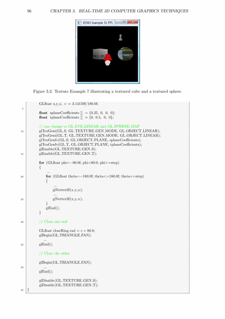
96 CHAPTER 3. REAL-TIME 3D COMPUTER GRAPHICS TECHNIQUES
Figure 3.2: Texture Example 7 illustrating a textured cube and a textured sphere.
GLfloat x,y,z, c = 3.14159f/180.0f;5
float splaneCoefficients [] = {0.25, 0, 0, 0};float tplaneCoefficients [] = {0, 0.5, 0, 0};
// can change to GL EYE LINEAR and GL SPHERE MAP10 glTexGeni(GL S, GL TEXTURE GEN MODE, GL OBJECT LINEAR);
glTexGeni(GL T, GL TEXTURE GEN MODE, GL OBJECT LINEAR);glTexGenfv(GL S, GL OBJECT PLANE, splaneCoefficients);glTexGenfv(GL T, GL OBJECT PLANE, tplaneCoefficients);glEnable(GL TEXTURE GEN S);
15 glEnable(GL TEXTURE GEN T);
for (GLfloat phi=−80.0f; phi<80.0; phi+=step){
...20 for (GLfloat theta=−180.0f; theta<=180.0f; theta+=step)
{...glVertex3f(x,y,z );...
25 glVertex3f(x,y,z );}glEnd();
}
30 // Close one end
GLfloat closeRing rad = c ∗ 80.0;glBegin(GL TRIANGLE FAN);
...35 glEnd();
// Close the other
glBegin(GL TRIANGLE FAN);40 ...
glEnd();
glDisable(GL TEXTURE GEN S);glDisable(GL TEXTURE GEN T);
45 }

3.2. TEXTURE MAPPING IN OPENGL 97
Figure 3.3: Examples of the modifications of the s plane and t plane coefficients: In (a)we have s = [0.25, 0, 0, 0] and t = [0, 0.25, 0, 0], (b) we have have s = [0.125, 0, 0, 0] andt = [0, 0.125, 0, 0] and (c) we have s = [0.125, 0.125, 0, 0] and t = [0, 0.125, 0.125, 0].
Figure 3.4: Examples of the modifications to the texture generation mode. Figure 3.3(b)illustrates the situation when the GL TEXTURE GEN MODE is GL OBJECT LINEAR: In (a) wechange this to GL EYE LINEAR and in (b) to GL SPHERE MAP.

98 CHAPTER 3. REAL-TIME 3D COMPUTER GRAPHICS TECHNIQUES
Figure 3.5: Mipmapping examples: (a) illustrates several mipmaps of the same texture,starting with a 16x16 size, reducing to 8x8, 4x4 and a 2x2 version. (b) is not usingmipmaps and (c) is using mipmaps.
3.2.1 Mipmapping
When a scene is rendered in OpenGL textured objects are drawn at varying distancesfrom the viewpoint, some close and some distant. As a textured object moves away fromthe viewer the texture must be scaled down so it can be applied to the smaller object. Theproblem that arises from scaling the texture down is that as objects move further awayfrom the viewpoint the texture map may flicker due to this filtering. The solution to thisproblem is mipmapping. Mipmapping is the process by which a set of scaled texture mapsof decreasing resolution are generated from a single high resolution image and used toimprove accuracy during texture mapping. Each individual mipmap is a distinct texturethat looks like the original but is a down scaled version of the previous mipmap level.Mipmapping allows OpenGL to apply the appropriate level of detail for a texture whenrendering rather than involving shrinking the original image.
To generate and use these mipmaps we first generate each mipmap by taking half thesize of the previous mipmap and then scaling it. If we have a base image that is 64x64in size, the lower levels of detail will be 32x32, 16x16, 8x8, 4x4, 2x2 and 1x1. Thereare two ways to calculate the mipmaps and use them in OpenGL: by hand, or throughthe gluBuild2DMipmaps() function. If mipmaps are generated using your own algorithm,the glTexImage2D() function would be used with an increasing level parameter for eachsuccessive level of detail, with level 0 being the base texture level. More often than not,the gluBuild2DMipmaps() utility function will be used to generate a set of mipmaps for agiven texture. gluBuild2DMipmaps() will take care of scaling and uploading the mipmapsto memory. This utility function is the same as glTexImage2D(), except for the fact thatit builds mipmaps.
Once the different levels of detail have been generated they can be used to improve thequality of a textured object as OpenGL will automatically select the best level of detailto use for the texture without the involvement of the programmer. The mipmap that isselected can be defined with the glTexParameter() function. The trade off with mipmapsis that they will require additional texture memory and some extra computation must bemade to generate them.
3.3 Level of Detail (LOD)
The Level of Detail concept is that we can use more simple version of an object to representthat object when it is distant from the camera/viewer. Why would we do this? Well, onereason would be to preserve our frame rate... more triangles generally equates to a lowerframe rate. For example, if we were representing a person in a scene who was made upof 50,000 triangles, it would be possible to represent that person with a lot less triangles

3.3. LEVEL OF DETAIL (LOD) 99
Figure 3.6: LOD Example of a sphere with 40, 20, and 10 subdivisions
if they were only occupying 20-30 pixels of screen space - perhaps we could represent thedistant person by 1,000 triangles or less. A dodecahedron that we used before looks like asphere from a large enough distance and so can be used to replace it so long as it is viewedfrom this or a greater distance. However, if it must ever be viewed more closely, it willlook like a dodecahedron. If we decide to use the dodecahedron to stand in for a spherethen as the dodecahedron travels closer to the camera we must swap the dodecahedronwith a higher detailed sphere.
It is also possible to use other techniques such as fog to limit the depth of field andto allow us to ignore objects when we know that they will not be visible due to the foggyconditions. It is also more representative of the real-world, where a slight fog/haze limitsour viewing depth. In general LOD algorithms consist of three separate parts, which aregeneration, selection and switching.
Generation: One mechanism to generate different LOD models of the same objectwould be to do it manually by hand. However, the quality of the different models couldlead to noise when the different models are switched. Automated polygonal simplificationtools can be used for levels of detail generation. They removes primitives from an originalmesh in order to produce simpler models which retain the key visual characteristics of theoriginal object. The result is typically a series of simplifications (as shown in 3.6), whichcan be used in various conditions, such as in order to maintain a constant frame rate. Agood balance can be determined between the richness of the models and the time it takesto display them.
An alternative to LOD generation in certain cases is to use procedural modelling,which allows real-time detail to be added to a model as it is approached. One example ofthis is the use of fractals to model terrain, trees, plants within a scene. Such models aregenerated on-the-fly according to our procedural algorithm.
Selection is when we select which LOD is appropriate based on some criteria, such asdistance from the object or the area that the object will appear on the screen. A metric,called the benefit function, is evaluated for the current viewpoint and the currently locationof the object and the value of this function allows us to choose an appropriate LOD. Thereare different benefit functions, such as range-based that uses a user-defined distance valueto the object to decide if the object is visible and to what level of detail. An alternativeapproach is to use a project area-based LOD selection that often uses a bounding box todetermine the screen space coverage.
Switching is when we change from one LOD to another and is prone to sudden changes(called popping). The most straightforward switching mechanism is Discrete GeometryLOD where the different representations of the same object contain different numbers ofprimitives. The different LODs can be stored as indexed triangle strips and when requiredthe higher/lower level LOD is simply swapped into the next rendered frame. An alternativeapproach is to use a Blend LOD which performs a blend operation over a number of frames

100 CHAPTER 3. REAL-TIME 3D COMPUTER GRAPHICS TECHNIQUES
to smooth the transition. It is however much more computationally expensive.One LOD implementation could be as follows:
0 class Range{
float range;SceneObject∗ child;
public:5 Range(SceneObject∗ s, float r) { child = s; range = r; }
float getRange() { return range; }SceneObject∗ getChild() { return child; }
};
10 class LOD : public SceneObject{
private:std :: vector<Range> ∗rangeList;SceneObject ∗selectedChild;
15
public:LOD();virtual ˜LOD();virtual RTTI OBJECT TYPE getType() const { return RTTI LOD; }
20 void addChild(SceneObject∗ child, float range);
// Force every child to have a render and update methodsvirtual void render(float timeElapsed);virtual void postRender(float timeElapsed);
25 virtual void update(float timeElapsed);virtual void switchChild(float distance);
};
Where we have a Range class that contains a single scene object with a single rangevalue, i.e. the model that should be used at this range. The LOD class then contains avector of Range objects, again each object with its associated range value. The LOD classis a child of the SceneObject class so that it can be added as usual to the scene graph.There is a slight problem though - if we just add the different child objects as per usualthen how will the recursive tree parsing algorithm know which child to render and which toignore. It won’t, so for this (my) implementation we will have the LOD children separatedfrom the recursive tree parsing algorithm. This will allow the LOD object to still have itsown non-LOD children. Importantly, this is only one possible implementation and it maynot be suitable for all scene graph designs.
The implementation of the addChild() and switchChild(float) methods are as follows:
0 void LOD::addChild(SceneObject∗ child, float range){
Range r(child, range);rangeList−>push back(r);selectedChild = child;
5 }
void LOD::switchChild(float distance){
float curDist = 999999.0f;10 for(int i=0; i<rangeList−>size(); i++)
{// find object with smallest r that is greater than distanceRange range = rangeList−>at(i);float r = range.getRange();
15 SceneObject ∗o = range.getChild();

3.4. BILLBOARDING 101
if ((r <= curDist) && ( r >= distance)){
curDist = r;selectedChild = o;
20 }}
}
The addChild() method over-rides the parent addChild() method, but has differentarguments. This is due to the different organisational structure of the scene graph, allowingthe child object being added to the RangeList vector. The default selected child is thelast child that was added to the rangeList. The switchChild(float) method switches to thechild that is the most appropriate for the current distance between the viewer (camera)and the LOD object. This method implementation iterates through the rangeList vectorand finds the object with the smallest range that is closer than the distance between theviewer and the LOD object.
3.4 Billboarding
Billboarding is a technique by which we can render an image onto a polygon (the billboard)that is always facing the viewer. As the view changes the polygon orientation changes, butthe position remains the same (unless it changes for some other reason). Billboarding canbe used to represent effects such as smoke, fire, explosions, clouds etc. The data structureof a billboard is a polygon (usually a quadrilateral), a surface normal and an up direction.These two vectors (surface normal and up direction) are sufficient to describe the rotationrequired to place the polygon at its required orientation. The position of the billboard isthen described by a single point - possibly the centre of the polygon.
It would be usual for the surface normal ~n and the up vector ~u. One of these vectorsmust be maintained in the given direction. To create an orthonormal basis for the rotationmatrix we have to establish a set of three mutually perpendicular vectors to orient thebillboard. We have the normal direction ~n and the up vector ~u and can use these tocalculate a ’right’ vector by getting the cross-product of ~r = ~n × ~u. But, because the ~nand the up vector ~u are not necessarily orthogonal we can then use the new ~r vector withthe ~n vector to calculate the third orthogonal basis vector, using: ~u′ = ~r × ~n.
The new up vector can then be used to form a rotation matrix with the form: M =(~r, ~u′, ~n). A translation matrix can then be used to place this polygon in the requiredlocation. We still need to determine the method of calculating the up vector and surfacenormal for the billboard. There are several different types of billboard techniques:
• Screen-aligned billboard - The polygon that is used for the billboard is always parallelto the screen, the billboard’s normal vector is the negative of the view plane normal,and it has a constant up vector which is the same as the camera’s up vector.
• W orld-oriented billboard - Due to the nature of perspective projection objects thatare away from the view direction axis appear warped. This appears quite regular;however, it does not work well for screen-aligned billboarding as it does not distortcorrectly. World-oriented (viewpoint) billboarding makes the desired normal equalthe vector from the centre of the billboard to the viewer’s position and will distortthe billboard the same way as real geometry does.
• Axial billboard - Commonly used to represent trees axial billboarding has a fixedworld up vector in line with the trunk of the tree, but the texture normals do notface directly at the viewer, rather rotate around the trunk to align itself so as to facethe viewer as much as possible.
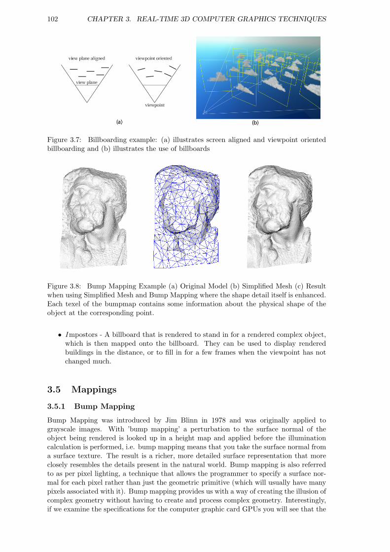
102 CHAPTER 3. REAL-TIME 3D COMPUTER GRAPHICS TECHNIQUES
Figure 3.7: Billboarding example: (a) illustrates screen aligned and viewpoint orientedbillboarding and (b) illustrates the use of billboards
Figure 3.8: Bump Mapping Example (a) Original Model (b) Simplified Mesh (c) Resultwhen using Simplified Mesh and Bump Mapping where the shape detail itself is enhanced.Each texel of the bumpmap contains some information about the physical shape of theobject at the corresponding point.
• Impostors - A billboard that is rendered to stand in for a rendered complex object,which is then mapped onto the billboard. They can be used to display renderedbuildings in the distance, or to fill in for a few frames when the viewpoint has notchanged much.
3.5 Mappings
3.5.1 Bump Mapping
Bump Mapping was introduced by Jim Blinn in 1978 and was originally applied tograyscale images. With ’bump mapping’ a perturbation to the surface normal of theobject being rendered is looked up in a height map and applied before the illuminationcalculation is performed, i.e. bump mapping means that you take the surface normal froma surface texture. The result is a richer, more detailed surface representation that moreclosely resembles the details present in the natural world. Bump mapping is also referredto as per pixel lighting, a technique that allows the programmer to specify a surface nor-mal for each pixel rather than just the geometric primitive (which will usually have manypixels associated with it). Bump mapping provides us with a way of creating the illusion ofcomplex geometry without having to create and process complex geometry. Interestingly,if we examine the specifications for the computer graphic card GPUs you will see that the

3.5. MAPPINGS 103
Figure 3.9: Emboss Bump Mapping
number of texels (texture elements) per second possible is roughly an order of magnitudelarger than the number of vertices per second possible. Figure 3.8 demonstrates the use ofbump mapping on a simplified mesh to illustrate that a similar level of detail can still berepresented on a greatly simplified geometric object. The visual illusion of the presencein the surface of small bumps, holes, irregularities, carvings, engraving, scales, and so on;if managed efficiently, this can be achieved at a very small fraction of the rendering timethat would be necessary for an object with similar characteristics modelled as geometry.Bump mapping does have drawbacks - in particular, bump mapping will lead to poorrendering of the silhouette as the object will still have a smooth geometry (rather thanthe perceived bumpy surface). There are two main techniques for Bump mapping:
• Emboss bump mapping
• Normal Mapping
Emboss bump mapping uses texture maps to generate bump mapping effects withoutrequiring a custom renderer. This multi-pass algorithm is an extension and refinementof texture embossing. The algorithm itself consists of: Render the image as a texture;Shift the texture coordinates at the vertices; and then Re-render the image as a texture,subtracting from the first image. In effect it duplicates the first texture, shifts it over thedesired amount of bump, darken the texture underneath, cut out the appropriate shapefrom the texture on top, and blend the two textures into one. This is called a two-passemboss bump mapping because it requires two textures. It is fairly simple to implement,but is applied to the diffuse lighting only and so displays poorly from certain angles. It isa good choice for planar surfaces (like the bricks in figure 3.9) and for 3D text displays.
Both bump maps and normal maps work by modifying the normal angle. Where Bumpmaps are textures that store an intensity, the relative height of pixels from the viewpoint ofthe camera (See figure 3.9) - Normal maps are images that store a direction, the directionof normals directly in the RGB values of an image (See figure 3.10)
Normal maps are also generated from heightmaps. It is the most common bumpmapping used today. Per pixel normals are represented in tangent space using a secondRGB texture (like on the RHS of figure 3.10).
However, we are combining (one representing normals, the other a conventional tex-ture) in a more sophisticated way. The tangent space refers to a co-ordinant system thatis relative to the current plane. That is, in tangent space, the normal vector (0,0,1) iscoincident with the normal of the geometry on which we are placing the the bump map.
You can think of bump maps as perturbing the direction of the geometric normal ateach pixel. The per pixel normals are encoded in an RGB texture map as described bytable 3.1.
To do bump mapping use an OpenGL 1.4 feature called texture combiners which pro-vide a texture environment for more sophisticated mixing of textures. Texture combinersallow multiple texture fragments to be combined. By default, you can simply choose oneof the texture environment modes (GL DECAL, GL REPLACE, GL MODULATE, or

104 CHAPTER 3. REAL-TIME 3D COMPUTER GRAPHICS TECHNIQUES
Figure 3.10: Normal Bump Mapping
RGB Encoding Tangent Space Comment127 127 127 0 0 0 The origin127 127 255 0 0 1 Straight up in the direction of geometric normal127 127 0 0 0 -1 Straight down, opposite of the geometric normal0 127 127 -1 0 0 -X direction in the plane255 127 127 1 0 0 +X direction in the plane127 0 127 0 -1 0 -Y direction in the plane127 255 127 0 1 0 +Y direction in the plane
Table 3.1: Encoding Texture Maps
GL ADD) for each texture unit, and the results of each texture application are thenadded to the next texture unit. Texture combiners add a new texture environment,GL COMBINE, that allows you to explicitly set the way texture fragments from eachtexture unit are combined. To use texture combiners, you call the glTexEnv function inthe following manner:
0 glTexEnvi(GL TEXTURE ENV, GL TEXTURE ENV MODE, GL COMBINE);
Texture combiners are controlled entirely through the glTexEnv function. You need toselect which texture combiner function you want to use, which can be either GL COMBINE RGBor GL COMBINE ALPHA. The third argument is the texture environment function thatyou want to employ (for either RGB or alpha values). For example, to select the GL REPLACEcombiner for RGB values, you would call the following function:
0 glTexEnvi(GL TEXTURE ENV, GL COMBINE RGB, GL REPLACE);
This combiner does little more than duplicate the normal GL REPLACE texture en-vironment. The following steps are required to perform bump mapping:
• Set up texture environment for the bump map (texture combiners).
• Set up texture environment for a second texture (if desired).
• Disable lighting.
• Calculate the light direction at each vertex and transform into RGB tangent spaceat each vertex of the geometry.
• Colour the vertex with this colour.
Set up texture environment for bump map (texture combiners):
0 glActiveTextureARB(GL TEXTURE0 ARB);glBindTexture(GL TEXTURE 2D,mybumptex);glEnable(GL TEXTURE 2D);glTexEnvf(GL TEXTURE ENV, GL TEXTURE ENV MODE,GL COMBINE EXT);glTexEnvf(GL TEXTURE ENV, GL COMBINE RGB EXT, GL DOT3 RGB EXT);

3.6. SHADOWS 105
Calculate the Light Direction: After the geometry to be bump mapped has beentransformed into place do:
0 glGetFloatv(GL MODELVIEW MATRIX, mv mat)glGetLightfv(GL LIGHT0, GL POSITION, lp vec)//gives us the position of the light in eye coordinates)
3.5.2 Displacement Mapping
Displacement mapping is a computer graphics technique in contrast to bump mappingthat uses a texture map to cause an effect where the actual geometric position of pointsover the textured surface are displaced along the local surface normal, according to thevalue the texture function evaluates to at each point on the surface. It gives surfaces agreater sense of depth and detail, permitting self-occlusion, self-shadowing and silhouettes.It is computationally expensive due to the large amount of additional geometry.
3.6 Shadows
Shading is a process used in drawing for depicting levels of darkness on paper by applyingmedia more densely or with a darker shade for darker areas, and less densely or with alighter shade for lighter areas. It is the process of altering a colour based on its angle tolights and its distance from lights to create a photorealistic effect. In contrast, shadowingis the process of creating a shadow by testing whether a pixel is visible from the lightsource, by comparing it to a z-buffer or depth image of the light source’s view, stored inthe form of a texture.
Umbra is the darkest part of a shadow where the source of light is completely concealedby the occluding object. Penumbra is the region where only a portion of the occludingbody is obscuring the light source (the outer part of the shadow).
3.6.1 Algorithms for Computing Shadows
z-buffer algorithm
This method follows directly from the idea that shadow points are hidden from light. Inother words, shadows are hidden surfaces from the point of view of a light. If we pretendthat the light point is the centre of projection (i.e. an eye point), we can render the scenefrom the light’s point of view, using a Z-buffer to compute surfaces visible to the light.The Z-buffer resulting from this will record all of the points that are closest to the light.Any point that has a further value at a given pixel is invisible to the light and hence is inshadow. The algorithm involves 1:
Pre-computing phase: (for each light source)
• Make light point the centre of projection.
• Calculate the transformation matrices.
• Transform object using light point matrices.
• Render object using z-buffer - lighting is skipped
• Save computed zbuffer depth info
Object rendering phase:
• Make eye point be centre of projection.1This discussion on shadows is modified from: http://web.cs.wpi.edu/~matt/courses/cs563/talks/
shadow/shadow.html
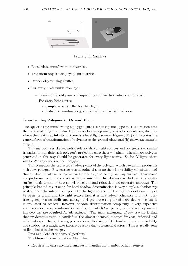
106 CHAPTER 3. REAL-TIME 3D COMPUTER GRAPHICS TECHNIQUES
L
S
P
(A) (B)
Figure 3.11: Shadows
• Recalculate transformation matrices.
• Transform object using eye point matrices.
• Render object using zbuffer.
• For every pixel visible from eye:
– Transform world point corresponding to pixel to shadow coordinates.
– For every light source:
∗ Sample saved zbuffer for that light.∗ if shadow coordinates ≤ zbuffer value - pixel is in shadow
Transforming Polygons to Ground Plane
The equations for transforming a polygon onto the z = 0 plane, opposite the direction thatthe light is shining from. Jim Blinn describes two primary cases for calculating shadowswhere the light is at infinity or there is a local light source. Figure 3.11 (a) illustrates thegeneral form of transformation of polygons to the ground plane and (b) shows an exampleoutput.
This method uses the geometric relationship of light sources and polygons, i.e. similartriangles, to calculate each polygon’s projection onto the z = 0 plane. The shadow polygongenerated in this way should be generated for every light source. So for N lights therewill be N projections of each polygon.
This computes the projected shadow points of the polygon, which we can fill, producinga shadow polygon. Ray casting was introduced as a method for visibility calculation andshadow determination. A ray is cast from the eye to each pixel, ray surface intersectionsare performed and the surface with the minimum hit distance is declared the visiblesurface. This technique also models reflection and refraction and generates shadows. Theprinciple behind ray tracing for hard shadow determination is very simple a shadow rayis shot from the intersection point to the light source. If the ray intersects any objectbetween its origin and the light source then it is in shadow, otherwise it is not. Raytracing requires no additional storage and pre-processing for shadow determination; itis evaluated as needed. However, shadow determination complexity is very expensiveand uses no coherence information with a cost of O(En) per ray shot, since ray surfaceintersections are required for all surfaces. The main advantage of ray tracing is thatshadow determination is handled in the almost identical manner for cast, reflected andrefracted rays. The ray tracing process is very floating point intensive. Thus, the visibilityand shadow tests might give incorrect results due to numerical errors. This is usually seenas little holes in the images.
Pros and Cons of the two Algorithms:The Ground Transformation Algorithm
• Requires no extra memory, and easily handles any number of light sources.

3.6. SHADOWS 107
• However, it only shadows onto ground plane, so it cannot handle objects whichshadow other complex objects.
• Every polygon is rendered N times, where N is number of light sources.
The Z-Buffer Algorithm
• Can shadow any scene which can be rendered using Z-buffer.
• However, it requires a separate memory buffer for each light source.
• Again, every polygon is rendered N times, where N is number of light sources, butN − 1 views do not need lighting calculations.
The Z-buffer algorithm is more versatile, with its ability to add shadows to scenes ofarbitrary complexity. Also, the precomputed shadow buffers can be used to render viewsfrom any eye point as long as the relative positions of the lights and objects are constantbetween these views. However, if memory resources are limited, the ground transformationalgorithm produces pleasing results if only ground shadowing is required.

108 CHAPTER 3. REAL-TIME 3D COMPUTER GRAPHICS TECHNIQUES
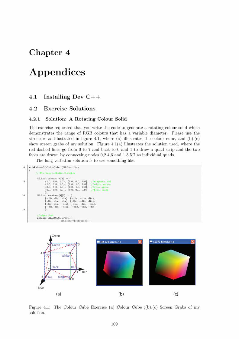
Chapter 4
Appendices
4.1 Installing Dev C++
4.2 Exercise Solutions
4.2.1 Solution: A Rotating Colour Solid
The exercise requested that you write the code to generate a rotating colour solid whichdemonstrates the range of RGB colours that has a variable diameter. Please use thestructure as illustrated in figure 4.1, where (a) illustrates the colour cube, and (b),(c)show screen grabs of my solution. Figure 4.1(a) illustrates the solution used, where thered dashed lines go from 0 to 7 and back to 0 and 1 to draw a quad strip and the twofaces are drawn by connecting nodes 0,2,4,6 and 1,3,5,7 as individual quads.
The long verbatim solution is to use something like:0 void drawGLColorCube1(GLfloat dia)
{// The long verbatim Solution
GLfloat colours [8][3] = {5 {1.0, 0.0, 1.0}, {1.0, 0.0, 0.0}, //magenta ,red
{1.0, 1.0, 1.0}, {1.0, 1.0, 0.0}, //white, yellow{0.0, 1.0, 1.0}, {0.0, 1.0, 0.0}, //cyan ,green{0.0, 0.0, 1.0}, {0.0, 0.0, 0.0} //blue, black};
10 GLfloat vertices [8][3] = {{−dia, dia, dia}, {−dia, −dia, dia},{ dia, dia, dia}, { dia, −dia, dia},{ dia, dia, −dia}, { dia, −dia, −dia},{−dia, dia, −dia}, {−dia, −dia, −dia}
15 };
//edges firstglBegin(GL QUAD STRIP);
glColor3fv(colours [0]);
(a) (b) (c)
Green
Blue
Red
Yellow
White
Red
Magenta
Cyan
Blue
Green
Black
1
2
0
3
4
5
6
7
Figure 4.1: The Colour Cube Exercise (a) Colour Cube ;(b),(c) Screen Grabs of mysolution.
109

110 CHAPTER 4. APPENDICES
20 glVertex3fv( vertices [0]);
glColor3fv(colours [1]);glVertex3fv( vertices [1]);
25 glColor3fv(colours [2]);glVertex3fv( vertices [2]);
glColor3fv(colours [3]);glVertex3fv( vertices [3]);
30glColor3fv(colours [4]);glVertex3fv( vertices [4]);
glColor3fv(colours [5]);35 glVertex3fv( vertices [5]);
glColor3fv(colours [6]);glVertex3fv( vertices [6]);
40 glColor3fv(colours [7]);glVertex3fv( vertices [7]);
glColor3fv(colours [0]);glVertex3fv( vertices [0]);
45glColor3fv(colours [1]);glVertex3fv( vertices [1]);
glEnd();
50 // then topglBegin(GL QUADS);
glColor3fv(colours [0]);glVertex3fv( vertices [0]);
55 glColor3fv(colours [2]);glVertex3fv( vertices [2]);
glColor3fv(colours [4]);glVertex3fv( vertices [4]);
60glColor3fv(colours [6]);glVertex3fv( vertices [6]);
glEnd();
65 //then bottomglBegin(GL QUADS);
glColor3fv(colours [1]);glVertex3fv( vertices [1]);
70 glColor3fv(colours [3]);glVertex3fv( vertices [3]);
glColor3fv(colours [5]);glVertex3fv( vertices [5]);
75glColor3fv(colours [7]);glVertex3fv( vertices [7]);
glEnd();}
which can be called by drawGLColorCube(0.5f);, but we could also introduce arraysof arrays as look up tables strip, which draws the four sides of the cube as a quad stripand topandbottom which draws two separate quads.
0 void drawGLColorCube2(GLfloat dia){
// The long verbatim SolutionGLfloat colours [8][3] = {
{1.0, 0.0, 1.0}, {1.0, 0.0, 0.0}, //magenta ,red5 {1.0, 1.0, 1.0}, {1.0, 1.0, 0.0}, //white, yellow
{0.0, 1.0, 1.0}, {0.0, 1.0, 0.0}, //cyan ,green{0.0, 0.0, 1.0}, {0.0, 0.0, 0.0} //blue, black};
GLfloat vertices [8][3] = {10 {−dia, dia, dia}, {−dia, −dia, dia},
{ dia, dia, dia}, { dia, −dia, dia},{ dia, dia, −dia}, { dia, −dia, −dia},{−dia, dia, −dia}, {−dia, −dia, −dia}};
15 int strip [10] = {0, 1, 2, 3, 4, 5, 6, 7, 0, 1};int topandbottom[8] = {0, 2, 4, 6, 1, 3, 5, 7 };
//edges firstglBegin(GL QUAD STRIP);
20 for(int i=0; i<10; i++){
glColor3fv(colours [ strip [ i ]]);glVertex3fv( vertices [ strip [ i ]]);
}25 glEnd();
// then top and bottomglBegin(GL QUADS);
for(int i=0; i<8; i++){
30 glColor3fv(colours [topandbottom[i]]);glVertex3fv( vertices [topandbottom[i]]);
}glEnd();
}

4.2. EXERCISE SOLUTIONS 111
There is a more advanced solution to this problem that uses Vertex Arrays, whichallow us to encapsulate the information in our cube structure and draw it using only asmall number of function calls. When using this approach it first has to be enabled usingthe glEnableClientState() function to enable the arrays that we wish to use. Thesearrays reside on the client side (rather than in the OpenGL state machine). We thenmust identify where the arrays are using the glVertexPointer() and glColorPointer()functions. The parameters in these functions specify (in order) the number of dimensions,the type of the data, that the elements are contiguous in memory and finally the pointerto the array of data. Finally we need to draw the elements themselves: Here we useGL POLYGON to draw the six faces of the cube, where the vertex indices are given in thecubeIndex array. This array has 24 elements, broken into 6 groups of 4 vertices. TheglDrawElements() function can be called to draw each face, where the parameters specify,the way to draw GL POLYGON, the number of elements that we wish to draw (4 in the caseof GL POLYGON), the type of data contained in the index array and finally a pointer thatpoints to the next index to use (in this case we wish to use 4 vertices then skip to the next4 etc.).
0 void drawGLColorCube3(GLfloat dia){
// enable the arrays on the client sideglEnableClientState(GL COLOR ARRAY);glEnableClientState(GL VERTEX ARRAY);
5GLfloat colours [8][3] = {
{1.0, 0.0, 1.0}, {1.0, 0.0, 0.0}, //magenta ,red{1.0, 1.0, 1.0}, {1.0, 1.0, 0.0}, //white, yellow{0.0, 1.0, 1.0}, {0.0, 1.0, 0.0}, //cyan ,green
10 {0.0, 0.0, 1.0}, {0.0, 0.0, 0.0} //blue, black};
GLfloat vertices [8][3] = {{−dia, dia, dia}, {−dia, −dia, dia},{ dia, dia, dia}, { dia, −dia, dia},
15 { dia, dia, −dia}, { dia, −dia, −dia},{−dia, dia, −dia}, {−dia, −dia, −dia}};
// identify where the arrays are20 glVertexPointer(3, GL FLOAT, 0, vertices);
glColorPointer(3, GL FLOAT, 0, colours);
GLubyte cubeIndex[24] = { 0, 1, 3, 2,2, 3, 5, 4,
25 4, 5, 7, 6,6, 7, 1, 0,0, 2, 4, 6, //top1, 3, 5, 7}; //bottom
for(int i=0; i<6; i++)30 {
// Draw the cube elementsglDrawElements(GL POLYGON, 4, GL UNSIGNED BYTE, &cubeIndex[4∗i]);
}}
We can even make this section of code shorter; the creation of the arrays and theintialisation of the state do not need to be called each time the cube is rotated and drawn,hence it would be possible to place these lines of code in the intialisation phase of theprogram and only call the glDrawElements() function 6 times in the drawGLColorCube3()function. And to be perfectly correct as each face of the cube is a quadrilateral it is possibleto use GL QUADS rather than GL POLYGON to draw the cube using this line of code:
0 glDrawElements(GL QUADS, 24, GL UNSIGNED BYTE, cubeIndex);
because GL QUADS starts a new quadrilateral after each four vertices.